Objective Variables for Probabilistic Revenue Maximization in Second-Price Auctions with Reserve

Abstract

Many online companies sell advertisement space in second-price auctions with reserve. In this paper, we develop a probabilistic method to learn a profitable strategy to set the reserve price. We use historical auction data with features to fit a predictor of the best reserve price. This problem is delicate—the structure of the auction is such that a reserve price set too high is much worse than a reserve price set too low. To address this we develop objective variables, a new framework for combining probabilistic modeling with optimal decision-making. Objective variables are ”hallucinated observations” that transform the revenue maximization task into a regularized maximum likelihood estimation problem, which we solve with an EM algorithm. This framework enables a variety of prediction mechanisms to set the reserve price. As examples, we study objective variable methods with regression, kernelized regression, and neural networks on simulated and real data. Our methods outperform previous approaches both in terms of scalability and profit.

1 Introduction

Many online companies earn money from auctions, selling advertisement space or other items. One widely used auction paradigm is second-price auctions with reserve [1]. In this paradigm, the company sets a reserve price, the minimal price at which they are willing to sell, before potential buyers cast their bids. If the highest bid is smaller than the reserve price then there is no transaction; the company does not earn money. If any bid is larger than the reserve price then the highest bidding buyer wins the auction, and the buyer pays the larger of the second highest bid and the reserve price. To maximize their profit from a specific auction, the host company wants to set the reserve price as close as possible to the (future, unknown) highest bid, but no higher.

Imagine a company which hosts second-price auctions with reserve to sell baseball cards. This auction mechanism is designed to be incentive compatible [2], which means that it is advantageous for baseball enthusiasts to bid exactly what they are willing to pay for the Stanley Kofax baseball card they are eager to own. Before each auction starts the company has to set the reserve price. When companies run millions of auctions of similar items, they have the opportunity to learn how to opportunistically set the reserve price from their historical data. In other words, they can try to learn their users’ value of different items, and take advantage of this knowledge to maximize profit. This is the problem that we address in this paper.

We develop a probabilistic model that predicts a good reserve price from prior features of an auction. These features might be properties of the product, such as the placement of the advertisement, properties of the potential buyers, such as each one’s average past bids, or other external features, such as time of day of the auction. Given a data set of auction features and bids, our method learns a predictor of reserve price that maximizes the profit of future auctions.

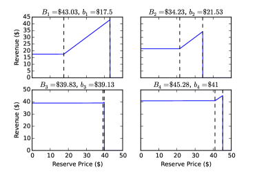
(a) Revenue function of $4$ auctions from the eBay data set as a function of reserve price. In second-price auctions with reserve the revenue depends on the highest and the second highest bid (dashed lines).

(b) The effect of smoothing on the revenue function of an auction from the eBay data set. The smaller $\sigma$ the closer the smoothed revenue approximates the actual revenue function.

Figure 1: The revenue (a) and smoothed revenue (b) for example auctions from the eBay data set.

A typical solution to such real-valued prediction problems is linear regression. However, the solution to this problem is more delicate. The reason is that the revenue function for each auction—the amount of money that we make as a function of the reserve price $y$—is asymmetric. It remains constant to the second-highest bid $b$, increases to the highest bid $B$, and is zero beyond the highest bid. Formally,

$$R(y,B,b)=\begin{cases}b&\text{ if }y<b\\ y&\text{ if }b\leq y\leq B\\ 0&\text{ otherwise}\end{cases}.$$ (1)

Fig. 1(a) illustrates this function for four auctions of sports collectibles from eBay. This figure puts the delicacy into relief. The best reserve price, in retrospect, is the highest bid $B$. But using a regression to predict the reserve price, e.g., by using the highest bid as the response variable, neglects the important fact that overestimating the reserve price is much worse than underestimating it. For example, consider the top left panel in Fig. 1(a), which might be the price of a Stanley Kofax baseball card. (Our data are anonymized, but we we use this example for concreteness.) The best reserve price in retrospect is $43.03. A linear regressor is just as likely to overestimate as to underestimate and hence fails to reflect that setting the price in advance to $44.00 would yield zero earnings while setting it to $40.00 would yield the full reserve.

To solve this problem we develop a new idea, the objective variable. Objective variables use the machinery of probabilistic models to reason about difficult prediction problems, such as one that seeks to optimize Eq.1. Specifically, objective variables enable us to formulate probabilistic models for which MAP estimation directly uncovers profitable decision-making strategies. We develop and study this technique to set the reserve price in second-price auctions.

In more detail, our aim is to find a parameterized mechanism $f(x_{i};w)$ to set the reserve price from the auction features $x_{i}$. In our study, we will consider a linear predictor, kernelized regression, and a neural network. We observe a historical data set of $N$ auctions that contains features $x_{i}$, and the auction’s two highest bids $B_{i}$ and $b_{i}$; we would like to learn a good mechanism by optimizing the parameter $w$ to maximize the total (retrospective) revenue $\sum_{i=1}^{N}R(f(x_{i};w),B_{i},b_{i})$.

We solve this optimization problem by turning it into a maximum a posteriori (MAP) problem. For each auction we define new binary variables—these are the objective variables—that are conditional on a reserve price. The probability of the objective variable being on (i.e., equal to one) is related to the revenue obtained from the reserve price; it is more likely on if the auction produces more revenue. We then set up a model that first assumes each reserve price is drawn from the parameterized mechanism $f(x_{i};w)$ and then draws the corresponding objective variable. Note that this model is defined conditioned on our data, the features and the bids. It is a model of the objective variables.

With the model defined, we now imagine a “data set” where all of the objective variables are on, and then fit the parameters $w$ subject to these data. Because of how we defined the objective variables, the model will prefer more profitable settings of the parameters. With this set up, fitting the parameters by MAP estimation is equivalent to finding the parameters that maximize revenue.

The spirit of this technique is that the objective variables are likely to be on when we make good decisions, that is, when we profit from our setting of the reserve price. When we imagine that they are all on, we are imagining that we made good decisions (in retrospect). When we fit the parameters to these data, we are using MAP estimation to find a mechanism that helps us make such decisions.

We first derive our method for linear predictors of reserve price and show how to use the expectation-maximization algorithm [3] to solve our MAP problem. We then show how to generalize the approach to nonlinear predictors, such as kernel regression and neural networks. Finally, on simulated data and real-world data from eBay, we show that this approach outperforms the existing methods for setting the reserve price. It is both more profitable and more easily scales to larger data sets.

Related work. Second-price auctions with reserve are first introduced in [1]. Ref. [4] empirically demonstrates the importance of optimizing reserve prices; Their study quantifies the positive impact it had on Yahoo!’s revenue. However, most previous work on optimizing the reserve price are limited in that they do not consider features of the auction [4, 5].

Our work builds on the ideas in Ref. [6]. This research shows how to learn a linear mapping from auction features to reserve prices, and demonstrates that we can increase profit when we incorporate features into the reserve-price setting mechanism. We take a probabilistic perspective on this problem, and show how to incorporate nonlinear predictors. We show in Sec. 3 that our algorithms scale better and perform better than these approaches.

The objective variable framework also relates to recent ideas from reinforcement learning to solve partially observable Markov decision processes (POMDPs) [7, 8]. Solving an POMDP amounts to finding an action policy that maximizes expected future return. Refs. [7, 8] introduce a binary reward variable (similar to an objective variable) and use maximum likelihood estimation to find such a policy. Our work solves a different problem with similar ideas, but there are also differences between the methods. In one way, the problem in reinforcement learning is more difficult because the reward is itself a function of the learned policy; in auctions, the revenue function is known and fixed. In addition, the work in reinforcement learning focuses on simple discrete policies while we show how to use these ideas for continuously parameterized predictors.

2 Objective Variables for Second-Price Auctions with Reserve

We first describe the problem setting and the objective. Our data come from previous auctions. For each auction, we observe features $x_{i}$, the highest bid $B_{i}$, and the second highest bid $b_{i}$. The features represent various characteristics of the auction, such as the date, time of day, or properties of the item. For example, one of the auctions in the eBay sport collectibles data set might be for a Stanley Kofax baseball card; its features include the date of the auction and various aspects of the item, such as its condition and the average price of such cards on the open market.

When we execute an auction we set a reserve price before seeing the bids; this determines the revenue we receive after the bids are in. The revenue function (Eq. 1), which is indexed by the bids, determines how much money we make as a function of the chosen reserve price. We illustrate this function for 4 auctions from eBay in Fig. 1(a). Our goal is to use the historical data to learn how to profitably set the reserve price from auction features, that is, before we see the bids.

For now we will use a linear function to map auction features to a good reserve price. Given the feature vector $x_{i}$, we set the reserve price with $f(x_{i};w)=w^{\top}x_{i}$. (In Sec. LABEL:nonlin we consider nonlinear alternatives.) We fit the coefficients $w$ from data, seeking $w$ that maximizes the regularized revenue

$$w^{*}=\operatorname*{arg\,max}\sum_{i=1}^{N}R(f(x_{i};w),B_{i},b_{i})+(\lambda/2)w^{\top}w.$$ (2)

We have chosen an $L_{2}$ regularization controlled by parameter $\lambda$; other regularizers are also possible.

Before we discuss our solution to this optimization, we make two related notes. First, the previous reserve prices are not included in the data. Rather, our data tell us about the relationship between features and bids. All the information about how much we might profit from the auction is in the revenue function; the way previous sellers set the reserve prices is not relevant. Second, our goal is not the same as learning a mapping from features to the highest bid. Not all auctions are made equal: Consider the top left auction in Fig. 1(a) with highest and second highest bid $B_{1}=\$43.03$ and $b_{1}=\$17.5$ compared to the bottom left auction in Fig. 1(a) with both highest and second highest bids almost identical at $B_{3}=\$39.83$ and $b_{3}=\$39.17$. The profit margin in the first auction is much larger, so predicting the reserve price for this auction well is much more important than when the two highest bids are close to each other. We account for this by directly maximizing revenue, rather than by modeling the highest bid.

2.1 The smoothed revenue

The optimization problem in Eq. 2 is difficult to solve because $R(\cdot)$ is discontinuous (and thus non-convex). Previous work [6] addresses this problem by iteratively fitting differences of convex (DC) surrogate functions and solving the resulting DC-program [9]. We define an objective function related to the revenue, but that smooths out the troublesome discontunuity. In the next section we show how to optimize this objective with an expectation-maximization algorithm.

We first place a Gaussian distribution on the reserve price centered around the linear mapping, $y_{i}\sim\mathcal{N}(f(x_{i};w),\sigma^{2})$. We define the smoothed regularized revenue to be

$$\mathcal{L}(w)=\sum_{i=1}^{N}\log\mathbb{E}_{y_{i}}\left[\exp\left\{-R(y_{i},B_{i},b_{i})\right\}\right]-(\lambda/2)w^{\top}w.$$ (3)

Figure 1(b) shows one term from Eq. 3 and how – for a specific auction – the smoothed revenue becomes closer to the original revenue function as $\sigma^{2}$ decreases. This approach was inspired by probit regression, where a Gaussian expectation is introduced to smooth the discontinuous 0-1 loss [10, 11].

We now have a well-defined and continuous objective function; in principle, we can use gradient methods to fit the parameters. However, we will fit them by recasting the problem as a regularized likelihood under a latent variable model and then using the expectation-maximization (EM) algorithm [3]. This leads to closed-form updates in both the E and M steps, and facilitates replacing linear regression with a nonlinear predictor.

2.2 Objective variables

To reformulate our optimization problem, we introduce the idea of the the objective variable. Objective variables are part of a probabilistic model for which MAP estimation recovers the parameter $w$ that maximizes the smoothed revenue in Eq. 3. Specifically, we define binary variables $z_{i}$ for each auction, each conditioned on the reserve price $y_{i}$, the highest bid $B_{i}$, and next bid $b_{i}$. We can interpret these variables to indicate “Is the auction host satisfied with the outcome?” Concretely, the likelihood of satisfaction is related to how profitable the auction was relative to the maximum profit, $p(z_{i}=1\,|\,y_{i},B_{i},b_{i})=\pi(y_{i},B_{i},b_{i})$ where

$$\pi(y_{i},B_{i},b_{i})=\exp\left\{-(B_{i}-R(y_{i},B_{i},b_{i}))\right\}.$$ (4)

The revenue function $R(\cdot)$ is in Eq. 1. The revenue is bounded by $B_{i}$; thus the probability is in $(0,1]$.

What we will do is set up a probability model around the objective variables, assume that they are all “observed” to be equal to one (i.e., we are satisfied with all of our auction outcomes), and then fit the parameter $w$ to maximize the posterior conditioned on this ”hallucinated data”. Fig. 2(b) provides visual intuition why the modes of the posterior are profitable. For fixed $w$ the posterior of $y_{i}$ is proportional to the product of its prior centered at $f(x_{i};w)$ and the likelihood of the objective variable (Eq. 4) which captures the profitability of each possible reserve price prediction.

Consider the following model,

$$w \sim\mathcal{N}(0,\lambda^{-1}I)$$ (5)

$$y_{i}\,|\,w,x_{i} \sim\mathcal{N}(f(x_{i};w),\sigma^{2})\quad i\in\{1,\ldots,N\}$$ (6)

$$z_{i}\,|\,y_{i},B_{i},b_{i} \sim\mathrm{Bernoulli}(\pi(y_{i},B_{i},b_{i}))$$ (7)

where $f(x_{i};w)=x_{i}^{\top}w$ is a linear map (for now). This is illustrated as a graphical model in Fig. LABEL:gm.

Now consider a data set $\mathbf{z}$ where all of the objective variables $z_{i}$ are equal to one. Conditional on this data, the log posterior of $w$ marginalizes out the latent reserve prices $y_{i}$,

$$\log p(w\,|\,\mathbf{z},\mathbf{x},\mathbf{B},\mathbf{b})=\log p(w\,|\,\lambda)+\sum_{i=1}^{N}\left(\log\mathbb{E}\left[\exp\{R(y_{i},B_{i},b_{i})\}\right]-B_{i}\right)-C,$$ (8)

where $C$ is the normalizer. This is the smoothed revenue of Eq. 3 plus a constant involving the top bids $B_{i}$ in Eq. 4, constant components of the prior on $w$, and the normalizer. Thus, we can optimize the smoothed revenue by taking MAP estimates of $w$.

(a) The objective variable model (OV model). The objective variable is shaded with diagonal lines to distinguish that its value is not observed but rather set to our desired value.

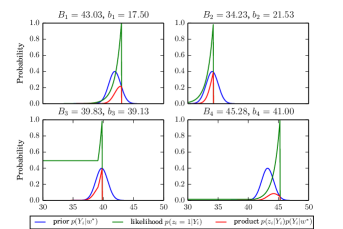
(b) For fixed w the posterior of the latent reserve price (red) is proportional to the prior (blue) times the likelihood of the objective (green). MAP estimation uncovers profitable modes of the posterior.

Figure 2: The objective variable framework transforms the revenue maximization task into a MAP estimation task. The model and the hallucinated data are designed such that the modes of the model’s posterior are the local maxima of the smoothed revenue in Eq. 3

.

As we mentioned above, we have defined variables corresponding to the auction host’s satisfaction. With historical data of auction attributes and bids, we imagine that the host was satisfied with every auction. When we fit $w$, we ask for the reserve-price-setting mechanism that leads to such an outcome.

2.3 MAP estimation with expectation-maximization

The EM algorithm is a technique for maximum likelihood estimation in the face of hidden variables [3]. (When there are regularizers, it is a technique for MAP estimation.) In the E-step, we compute the posterior distribution of the hidden variables given the current model settings; in the M-step, we maximize the expected complete regularized log likelihood, where the expectation is taken with respect to the previously computed posterior.

In the OV model, the latent variables are the reserve prices $\mathbf{y}$; the observations are the objective variables $\mathbf{z}$; and the model parameters are the coefficients $w$. We compute the posterior expectation of the latent reserve prices in the E-step and fit the model parameters in the M-step. This is a coordinate ascent algorithm on the expected complete regularized log likelihood of the model and the data. Each E-step tightens the bound on the likelihood and the new bound is then optimized in the M-step.

E-step. At iteration $t$, the E-step computes the conditional distribution of the latent reserve prices $y_{i}$ given the objective variables $z_{i}=1$ and the parameters $w^{(t-1)}$ of the previous iteration. It is

$$p(y_{i}|z_{i}=1,w^{(t-1)}) \propto p(z_{i}=1|y_{i})p(y_{i}|w^{(t-1)})$$ (9)

$$\propto\exp\left\{-(B_{i}-R(y_{i},B_{i},b_{i})\right\}\phi\left(\frac{y_{i}-f(x_{i};w^{(t-1)})}{\sigma}\right).$$ (10)

where $\phi(\cdot)$ is the pdf of the standard normal distribution. The normalizing constant is in the appendix in Eq. 15; we compute it by integrating Eq. 9 over the real line. We can then compute the posterior expectation $\mathbb{E}\left[y_{i}\,|\,z_{i},w^{(t-1)}\right]$ by using the moment generating function. (See Eq. 18,Sec. A)

M-step. The M-step maximizes the complete joint log-likelihood with respect to the model parameters $w$. When we use a linear predictor to set the reserve prices, i.e. $f(x_{i};w)=x_{i}^{\top}w$, the M-step has a closed form update, which amounts to ridge regression against response variables $\mathbb{E}\left[y_{i}\,|\,z_{i},w^{(t-1)}\right]$ (Eq. 18) computed in the E-step. The update is

$$w^{(t)}=\left(\lambda I+\frac{1}{\sigma^{2}}\mathbf{x}^{\top}\mathbf{x}\right)^{-1}\frac{1}{\sigma^{2}}\mathbf{x}^{\top}\mathbb{E}\left[\mathbf{y}\,|\,\mathbf{z},w^{(t-1)}\right]$$ (11)

where $\mathbb{E}\left[\mathbf{y}\,|\,\mathbf{z},w^{(t-1)}\right]$ denotes the vector with $i^{th}$ entry $\mathbb{E}\left[y_{i}\,|\,\mathbf{z},w^{(t-1)}\right]$ and similarly $\mathbf{x}$ is a matrix of all feature vectors $x_{i}$.

Algorithm details. To initialize, we set the expected reserve prices to be the highest bids $\mathbb{E}[y_{i}\,|\,z_{i}]=B_{i}$ and run an M-step. The algorithm then alternates between updating the weights using Eq. 11 in the M-step and then integrating out the latent reserve prices in the E-step. The algorithm terminates when the change in revenue on a validation set is below a threshold. (We use $10^{-5}$.)

The E-step is linear in the number of auctions $N$ and can be parallelized since the expected reserve prices are conditionally independent in our model. The least squares update has asymptotic complexity $O(d^{2}N)$ where $d$ is the number of features.

2.4 Nonlinear Objective Variable Models

One of the advantages of our EM algorithm is that we can change the parameterized prediction technique $f(x_{i};w)$ from which we map auction features to the mean of the reserve price. So far we have only considered linear predictors; here we show how we can adapt the algorithm to nonlinear predictors. As we will see in Sec. 3, these nonlinear predictors outperform the linear predictors.

In our framework, much of the model in Fig. 2(a) and corresponding algorithm remains the same even when considering nonlinear predictors. The distribution of the objective variables is unchanged (Eq. 4) as well as the E-step update in the EM algorithm (Eq. 18). All of the changes are in the M-step.

Kernel regression. Kernel regression [12] maps the features $x_{i}$ into a higher dimensional space through feature map $\psi(\cdot)$; the mechanism for setting the reserve price becomes $f(x_{i};w)=\psi(x_{i})^{T}w$. In kernel regression we work with the $N\times N$ Gram matrix $K$ of inner products, where $K_{ij}=\psi(x_{i})^{T}\psi(x_{j})$. In this work we use a polynomial kernel of degree $D$, and thus compute the gram matrix without evaluating the feature map $\psi(\cdot)$ explicitly, $K=(\mathbf{x}^{\top}\mathbf{x}+1)^{D}$.

Rather than learning the weights directly, kernel methods operate in the dual space $\alpha\in\mathbb{R}^{N}$. If $K_{i}$ is the $i^{th}$ column of the Gram matrix, then the mean of the reserve price is

$$f(x_{i};w)=\psi(x_{i})^{T}w=K_{i}^{T}\alpha.$$ (12)

The corresponding M-step in the algorithm becomes

$$\alpha^{(t)}=\left(\frac{1}{\sigma^{2}}K+\lambda I_{N}\right)^{-1}\frac{1}{\sigma^{2}}\mathbb{E}[\mathbf{y}\,|\,\mathbf{z},\alpha^{(t-1)}].$$ (13)

See [13] for the technical details around kernel regression.

We will demonstrate in Sec. 3 that replacing linear regression with kernel regression can lead to better reserve price predictions. However, working with the Gram matrices comes at a computational cost and we consider neural networks as a scalable alternative to infusing nonlinearity into the model.

Neural networks. We also explore an objective variable model that uses a neural network [14] to set the mean reserve prices. We use a network with one hidden layer of $H$ units and activation function $\tanh(\cdot)$. The parameters of the neural net are the weights of the first layer and the second layer: $w=\{w^{(1)}\in\mathbb{R}^{H\times d},w^{(2)}\in\mathbb{R}^{1\times H}\}$. The mean of the reserve price is

$$f(x_{i};w)=w^{(2)}(\tanh(w^{(1)}x_{i})).$$ (14)

The M-step is no longer analytic; Instead, the network is trained using stochastic gradient methods.

3 Empirical Study

Table 1: The performance of the EM algorithms from Sec. 2 (OV Regression, OV Kernel Regression with degree $2$ and $4$, OV Neural Networks) against the current state of the art (DC [6] and NoF [5]). We report results in terms of percentage of maximum possible revenue (computed by an oracle that knows the highest bid in advance). For each data set, we report mean and standard error aggregated from ten train/validation/test splits. Our methods outperform the existing methods on all data.

	OV Reg	OV Kern (2)	OV Kern (4)	OV NN	DC [6]	NoF [5]
Linear Sim.	$\mathbf{81.4\pm 0.2}$	$81.2\pm 0.2$	$78.2\pm 0.6$	$72.2\pm 1.5$	$80.3\pm 0.3$	$49.9\pm 0.1$
Nonlinear Sim.	$50.3\pm 0.3$	$66.2\pm 0.4$	$\mathbf{70.1\pm 0.6}$	$63.7\pm 2.9$	$59.4\pm 2.0$	$49.9\pm 0.2$
eBay (s)	$61.0\pm 0.7$	$63.7\pm 3.0$	$63.4\pm 2.8$	$\mathbf{74.4\pm 1.1}$	$59.5\pm 1.1$	$55.8\pm 0.3$
eBay (L)	$62.4\pm 0.2$	-	-	$\mathbf{84.0\pm 0.2}$	-	$56.0\pm 0.1$

We studied our algorithms with two simulated data sets and a large collection of real-world auction data from eBay. In each study, we fit a model on a subset of the data (using a validation set to set hyperparameters) and then test how profitable we would be if we used the fitted model to set reserve prices in a held out set. Our objective variable methods outperformed the existing state of the art.

Data sets and replications. We evaluated our method on both simulated data and real-world data.

• Linear simulated data. Our simplest simulated data contains $d=5$ auction features. We drew features $x_{i}\sim N(0,I)\in\mathbb{R}^{d}$ for 2,000 auctions; we drew a ground truth weight vector $\hat{w}\sim\mathcal{N}(0,I)\in\mathbb{R}^{d}$ and an intercept $\alpha\sim\mathcal{N}(0,1)$; we drew the highest bids for each auction from the regression $B_{i}\sim\mathcal{N}(w^{\top}x_{i}+\alpha,0.1)$ and set the second bids $b_{i}=B_{i}/2$. (Data for which $B_{i}$ is negative are discarded and re-drawn.) We split into $N_{\text{train}}=1000$ and $N_{\text{valid}}=N_{\text{test}}=500$.

• Nonlinear simulated data. These data contain features $x_{i}$, true coefficients $\hat{w}$, and intercept $\alpha$ generated as for the linear data. We generate highest bids by taking the absolute value of those generated by the regression and second highest bids by halving them, as above. Taking the absolute value introduces a nonlinear relationship between features and bids.

• Data from eBay. Our real-world data is auctions of sports collectibles from eBay. There are $d=74$ features. All covariates are centered and rescaled to have mean zero and standard deviation one. We analyze two data sets from eBay, one small and one large. On the small data set, the total number of auctions is $6,000$, split into $N_{\text{train}}=N_{\text{valid}}=N_{\text{test}}=2,000$. On the large data set the total number is 70,000, split into $N_{\text{train}}=50,000$, and $N_{\text{valid}}=N_{\text{test}}=10,000$.

In our study, we fit each method on the training data, use the validation set to decide on hyperparameters, and then evaluate the fitted predictor on the test set, i.e., compute how much revenue we make when we use it to set reserve prices. For each data set, we replicate each study ten times, each time randomly creating the training set, test set, and validation set.

Algorithms. We describe the objective variable algorithms from Sec. 2, all of which we implemented in Theano [15, 16], as well as the two previous methods we compare against.

• OV Regression. OV Regression learns a linear predictor $w$ for reserve prices using the algorithm in Sec. 2.3. We find a good setting for the smoothing parameter $\sigma$ and regularization parameter $\lambda$ using grid search.

• OV Kernel Regression. OV Kernel Regression uses a polynomial kernel to predict the mean of the reserve price; we study polynomial kernels of degree 2 and 4.

• OV Neural Network. OV Neural Network fits a neural net for predicting the reserve prices. As we discussed in Sec. 2.4, the M-step uses gradient optimization; we used stochastic gradient ascent with a constant learning rate and early stopping [17]. Further, we used a warm-start approach, where the next M-step is initialized with the results of the previous M-step. We set the number of hidden units to $H=5$ for the simulated data and $H=100$ for the eBay data. We use grid search to set the smoothing parameter $\sigma$, the regularization parameters, the learning rate, the batch size, and the number of passes over the data for each M-step.

• Difference of Convex Functions (DC) [6]. The DC algorithm finds a linear predictor of reserve price with an iterative procedure based on DC-programming [9]. Grid search is used on the regularization parameter as well as the margin to select the surrogates for the auction loss.

• No Features (NoF) [5]. This is the state-of-the-art approach to set the reserve prices when we do not consider the auction’s features. The algorithm iterates over the highest bids in the training set and evaluates the profitability of setting all reserve prices to this value on the training set. Ref. [6] gives a more efficient algorithm based on sorting.

Results. Tab. 1 gives the results of our study. The metric is the percentage of the highest possible revenue, where an oracle anticipates the bids and sets the reserve price to the highest bid.

A trivial strategy (not reported) sets all reserve prices to zero, and thus earns the second highest bid on each auction. The algorithm using no features [5] does slightly better than this but not as well as the algorithms which use features. OV Regression [this paper] and DC [6] both fit linear mappings and exhibit similar performance. However, the DC algorithm does not scale to the large eBay data set.

The nonlinear OV algorithms (OV Kernel Regression and OV Neural Networks) outperform the linear models on the nonlinear simulated data and the real-world data. Note that the kernel algorithms do not scale to the large eBay data set because working with the Gram matrix becomes infeasible as the training set gets large. OV Neural Networks significantly outperforms the existing methods on the real-world data. This is a viable solution to maximizing profit from historical auction data.

4 Summary and Discussion

We developed the objective variable framework for combining probabilistic modeling with optimal decision making. We used this method to solve the problem of how to set the reserve price in second-price auctions. Our algorithms scaled better and outperformed the current state of the art on both simulated and real-world data.

Appendix A Appendix - Update Equations for EM

The normalizing constant $C_{i}$ of Eq. 9 can be computed by integrating Eq. 9 over the real line. Let $\mu_{i}=f(x_{i};w^{(t-1)})$. Up to a constant factor of $e^{B_{i}}$ the normalizing constant $C_{i}$ then equals

$$C_{i}e^{B_{i}}= \int_{-\infty}^{b_{i}}e^{b_{i}}\phi(\frac{y_{i}-\mu_{i}}{\sigma})dy_{i}+\int_{b_{i}}^{B_{i}}e^{y_{i}}\phi(\frac{y_{i}-\mu_{i}}{\sigma})+\int_{B_{i}}^{\infty}\phi(\frac{y_{i}-\mu_{i}}{\sigma})$$ (15)

$$= \sigma e^{b_{i}}\Phi(\frac{b_{i}-\mu_{i}}{\sigma})+\sigma e^{\mu_{i}+\frac{\sigma^{2}}{2}}\big{[}\Phi(\frac{B_{i}-(\mu_{i}+\sigma^{2})}{\sigma})-\Phi(\frac{b_{i}-(\mu_{i}+\sigma^{2})}{\sigma})\big{]}$$

$$+\sigma\big{[}1-\Phi(\frac{B_{i}-\mu_{i}}{\sigma})\big{]}.$$ (16)

Computing the expectation of the latent reserve price $\mathbb{E}[y_{i}]$ entails evaluating the moment generating function $M_{i}(s)=\mathbb{E}[e^{sy_{i}}]$, where expectation is taken w.r.t. the posterior $p(y_{i}|z_{i}=1,w^{(t-1)})$. Taking the derivative with respect to $s$ and setting $s=0$ then yields the desired expectation.

$$\mathbb{E}[y_{i}]= \frac{dM_{i}(s)}{ds}\bigg{|}_{s=0}$$ (17)

$$= \frac{\sigma e^{b_{i}}}{C_{i}}\mu_{i}\Phi(\frac{b_{i}-\mu_{i}}{\sigma})-\frac{\sigma^{2}e^{b_{i}}}{C_{i}}\phi(\frac{b_{i}-\mu_{i}}{\sigma})+\frac{\sigma}{C_{i}}(\mu_{i}+\sigma^{2})e^{\mu_{i}+\frac{\sigma^{2}}{2}}\Phi(\frac{B_{i}-(\mu_{i}+\sigma^{2})}{\sigma})$$

$$-\frac{\sigma}{C_{i}}(\mu_{i}+\sigma^{2})e^{\mu_{i}+\frac{\sigma^{2}}{2}}\Phi(\frac{b_{i}-(\mu_{i}+\sigma^{2})}{\sigma})+\frac{\sigma}{C_{i}}\mu_{i}\big{[}1-\Phi(\frac{B_{i}-\mu_{i}}{\sigma})\big{]}$$

$$-\frac{\sigma^{2}}{C_{i}}e^{\mu_{i}+\frac{\sigma^{2}}{2}}\big{[}\phi(\frac{B_{i}-(\mu_{i}+\sigma^{2})}{\sigma})-\phi(\frac{b_{i}-(\mu_{i}+\sigma^{2})}{\sigma})\big{]}+\frac{\sigma^{2}}{C_{i}}\phi(\frac{-\mu_{i}}{\sigma})$$ (18)

References

- Easley and Kleinberg [2010] D. Easley and J. Kleinberg. Networks, Crowds, and Markets: Reasoning About a Highly Connected World. Cambridge University Press, New York, NY, USA, 2010.
- Bar-Yossef et al. [2002] Z. Bar-Yossef, K. Hildrum, and F. Wu. Incentive-compatible online auctions for digital goods. In ACM-SIAM symposium on Discrete algorithms, pages 964–970, 2002.
- Dempster et al. [1977] A. Dempster, N. Laird, and D. Rubin. Maximum likelihood from incomplete data via the EM algorithm. Journal of the Royal Statistical Society, Series B, 39:1–38, 1977.
- Ostrovsky and Schwarz [2011] M. Ostrovsky and M. Schwarz. Reserve prices in internet advertising auctions: A field experiment. In ACM conference on Electronic commerce, pages 59–60, 2011.
- Cesa-Bianchi et al. [2013] N. Cesa-Bianchi, C. Gentile, and Y. Mansour. Regret minimization for reserve prices in second-price auctions. In ACM-SIAM Symposium on Discrete Algorithms, pages 1190–1204, 2013.
- Medina and Mohri [2014] A. Medina and M. Mohri. Learning theory and algorithms for revenue optimization in second price auctions with reserve. In International Conference on Machine Learning, 2014.
- Toussaint et al. [2006] M. Toussaint, S. Harmeling, and A. Storkey. Probabilistic inference for solving (po) mdps. 2006.
- Toussaint et al. [2008] M. Toussaint, L. Charlin, and P. Poupart. Hierarchical pomdp controller optimization by likelihood maximization. In UAI, volume 24, pages 562–570, 2008.
- Tao and An [1998] P. Tao and L. An. A dc optimization algorithm for solving the trust-region subproblem. SIAM Journal on Optimization, 8(2):476–505, 1998.
- Albert and Chib [1993] J. Albert and S. Chib. Bayesian analysis of binary and polychotomous response data. Journal of the American statistical Association, 88(422):669–679, 1993.
- Holmes et al. [2006] C. Holmes, L. Held, et al. Bayesian auxiliary variable models for binary and multinomial regression. Bayesian Analysis, 1:145–168, 2006.
- Aizerman et al. [1964] A. Aizerman, E. Braverman, and L. Rozoner. Theoretical foundations of the potential function method in pattern recognition learning. Automation and remote control, 25, 1964.
- Bishop et al. [2006] C. Bishop et al. Pattern recognition and machine learning, volume 4. springer New York, 2006.
- Bishop et al. [1995] C. Bishop et al. Neural networks for pattern recognition. 1995.
- Bergstra et al. [2010] J. Bergstra et al. Theano: a CPU and GPU math expression compiler. In Proceedings of the Python for Scientific Computing Conference (SciPy), June 2010. Oral Presentation.
- Bastien et al. [2012] F. Bastien et al. Theano: new features and speed improvements. Deep Learning and Unsupervised Feature Learning NIPS 2012 Workshop, 2012.
- Prechelt [2012] L. Prechelt. Early stopping - but when? In Neural Networks: Tricks of the Trade, pages 53–67. Springer, 2012.