Looking for bSM physics using top-quark polarization and decay-lepton kinematic asymmetries

Abstract

We explore beyond Standard Model (bSM) physics signatures in the $l+jets$ channel of $t\overline{t}$ pair production process at the Tevatron and the LHC. We study the effects of bSM physics scenarios on the top quark polarization and on the kinematics of the decay leptons. To this end, we construct asymmetries using the lepton energy and angular distributions. Further, we find their correlations with the top polarization, net charge asymmetry and top forward backward asymmetry. We show that when used together, these observables can help discriminate effectively between SM and different bSM scenarios which can lead to varying degrees of top polarization at the Tevatron as well as the LHC. We use two types of coloured mediator models to demonstrate the effectiveness of proposed observables, an $s$-channel axigluon and a $u$-channel diquark.

I Introduction

Most experimental observations at particle accelerators fit the Standard Model (SM) very well. However, there are some major puzzles to be solved. One needs to have physics beyond the standard model (bSM) to explain the presence of dark matter, explain quantitatively the observed baryon asymmetry of the universe, and to explain the puzzle of dark energy. Looking for signs of bSM, one finds that most of the terrestrial experimental observations that are in tension with the SM results are in the properties of third generation fermions. For example $B\to\tau\nu$ Lees:2012ju , $h\to\mu\tau$ CMS-PAS-HIG-14-005 and $b\overline{b}$ forward backward asymmetry (AFB) at LEP and Tevatron Abazov:2014ysa ; ALEPH:2005ab ; Murphy:2015cha show such deviations. One of these long standing puzzles is the top-quark AFB measured by the D0 and CDF detectors at the Tevatron collider in 2008 d02008afb ; cdf2008afb . These observations by two independent collaborations were updated with full data from the Tevatron and were consistent with each other and in tension with the SM calculations until 2015. Recent experimental results from $D0$ Abazov:2014cca and theoretical calculations Kidonakis:2015ona point towards the possibility that the anomalous nature of these observations may be a statistical phenomenon.

Due to its large mass which is close to the electroweak scale and the implied connection with electroweak symmetry breaking, the top quark is an important laboratory for various bSM searches at colliders. In fact various proposals put forward to solve the different theoretical problems of the SM often involve modifications in the top sector. Various extensions to the SM have also been proposed inspired by the possibly anomalous value of measured top-AFB at the Tevatron. These bSM proposals involve explanation of the AFB in terms of processes involving a) $s$-channel resonances like the axigluon, KK gluon, coloron DC:2007AfbAx ; Antunano:2007da ; Ferrario:2009ax ; framptonshu2010 ; DC:2010_W'z'Axdiq ; Dutta:2012ai ; Fajfer:2012si ; AguilarSaavedra:2011ug ; Gresham:2012kv or b) t-channel exchange of particles with different spin and SM charges like the $Z^{\prime}$ , diquarks etc Jung:2009_Z' ; Papaefstathiou:2011kd ; Fajfer:2012si ; Shu_Tait_2009diquark ; DC:2010_W'z'Axdiq ; Barger:2011W'Z' ; Rajaraman:2011rw ; Patel:2011eh ; Berger:2013ysa ; AguilarSaavedra:2011ug . Effective operator approach has also been used in this context effLag_Ko ; Franzosi:2015osa ; Biswal:2012mr . Measurements of other related observables such as lepton angular asymmetries and $t\bar{t}$ invariant-mass dependence of the top quark AFB are also compatible with the hypothesis of a heavy bSM particle, see for example Shu:2011au ; Westhoff:2013ixa .

In this study, we will focus on the lepton + jets final state ($p\overline{p}/pp\to t\overline{t}\to b\nu l\overline{t}$) of the $t\overline{t}$ pair production process. This channel has a larger cross-section as compared to the dilepton + jets channel, and it has a much smaller background compared to the all jets channel. For lighter quarks, hadronization smears the information available about their spin and polarization. The mass of the top quark is large enough that it decays into its daughter particles before strong interactions can initiate the hadronization process. Hence top-quark polarization leaves a memory in the kinematic distribution of the decay products and can be tracked Jezabek:1988topdecayleptondist ; Godbole:2006ldistandtpol . We study the correlations between various kinematic asymmetries and polarization to distinguish between different sources of these asymmetries within an $s$-channel (axigluon) and a $t$-channel (diquark) extension of the SM. For the Tevatron, the top pair production process is dominated by $q\overline{q}$ collisions and at the LHC it is dominated by $gg$ collisions which means that new physics can manifest at differently at the two colliders.

A wide variety of observables have been studied in the literature to explore the top sector as a bSM portal Antunano:2007da ; Fajfer:2012si ; Rajaraman:2011rw ; Bernreuther:2010ny ; AguilarSaavedra:2012rx ; Bernreuther:2012sx ; AguilarSaavedra:2012xe ; Hewett:2011wz . A brief review of some of these observables which have been experimentally measured and are relevant to this work is presented in section II. In section III,IV we describe the flavour non-universal axigluon and diquark models which we use as templates for our analysis. Constraints on these models from top pair production cross-section and forward backward asymmetry at Tevatron, charge asymmetry, top quark pair production, dijet and four jet production cross-sections at LHC are discussed in section V. In section VI we construct the asymmetries which we use to explore the bSM models. In section VII we present the correlations between various asymmetries and discuss the role of top quark polarization and kinematics in discerning the various regions of parameter space of the bSM models. We contrast our results for the axigluon and diquark models and the resulting conclusions can be generalized to other new physics scenarios. Our results are presented for the Tevatron $\sqrt{s}=1.96$ TeV and the LHC $\sqrt{s}=7$ TeV , $13$ TeV. We discuss the effects of transverse polarization coming from the off-diagonal terms in the top-quark density matrix in section VIII and then conclude in section IX.

II Status of experimental results

We begin by summarizing some of the experimental results from the LHC and the Tevatron concerning the top quark and compare them with the corresponding SM calculations from the literature.

The measured $t\bar{t}$ production cross-section for the Tevatron at $\sqrt{s}=1.96$ TeV is $\sigma_{p\overline{p}\to t\overline{t}}^{Tevatron}=7.60\pm 0.41$ pb Aaltonen:2013wca and that for the LHC at $\sqrt{s}=7$ TeV is $\sigma_{pp\to t\overline{t}}^{LHC}=173.30\pm 10.10$ pb CMS:2013sca ; ATLAS:2012dpa . These agree with the calculated SM NNLO cross-sections $\sigma_{p\overline{p}\to t\overline{t}}^{Tevatron}=7.16{}_{-0.50}^{+0.54}$ pb SM_tevatron_crs for the Tevatron, and $\sigma_{pp\to t\overline{t}}^{LHC\,7TeV}=177.30\pm 10.63$ pb Czakon:2011xx for the LHC, within $1\sigma$. The uncertainties coming from the top-quark mass dependence of $t\overline{t}$ cross-section Czakon:2013goa have been included in the given LHC cross-sections. In the calculations in following sections, we use a common K factor for the bSM+SM to estimate the NNLO total cross-section. For the Tevatron, the K factor is $K_{Tevatron}=1.39{}_{-0.10}^{+0.10}$ k_Tevatron . The K factor for the LHC is calculated using the NNLO cross-section cited above and LO cross-section calculated using CTEQ6l parton distribution functions (pdf) with factorization scale $Q=2m_{t}$. The errors in the K factors represent pdf uncertainties, scale dependence and statistical errors in the NNLO cross-section. For the LHC with $\sqrt{s}=7$ TeV, $K_{LHC7}=2.20_{-0.15}^{+0.14}$.

The cross-sections impose a constraint on any new particle to have small couplings with the top quark and/or have a sufficiently high mass. It is interesting to note that we can still find a range of couplings of the bSM large enough to explain the measured anomalous top-quark and lepton asymmetries reported at the Tevatron and remain compatible with the measurements at the LHC. The AFB of the top quark in the $t\overline{t}$ centre-of-mass (CM) frame is defined as

$$A_{Forward\,Backward} = \frac{N_{F}(y_{t}-y_{\bar{t}}>0)-N_{B}(y_{t}-y_{\bar{t}}<0)}{N_{F}(y_{t}-y_{\bar{t}}>0)+N_{B}(y_{t}-y_{\bar{t}}<0)}$$ (1)

$$= \frac{N(\cos\theta_{t}>0)-N(\cos\theta_{t}<0)}{N(\cos\theta_{t}>0)+N(\cos\theta_{t}<0)},$$ (2)

where $y_{t}$, $y_{\bar{t}}$ are respectively the rapidities of the $t$ and the $\bar{t}$ and $\theta_{t}$ and $\theta_{\bar{t}}$ are their respective polar angles measured with respect to the beam direction.

The CDF measurement of the $t\overline{t}$ CM frame AFB with the full data set is $A_{FB}^{t\bar{t}}=0.164\pm 0.045$ FBA_mttbar2013 . The corresponding SM result is 0 at tree level in QCD. At NLO in QCD, the value predicted is $0.0589_{-0.0140}^{+0.0270}$ (the errors only represent scale variation) which upon including NLO electroweak corrections becomes, $0.0734_{-0.0058}^{+0.0068}$ Czakon:2014xsa . Recently, AFB has been calculated at NNLO to be $0.0749_{-0.0086}^{+0.0049}$ in pure QCD and $0.095\pm 0.007$ including EW corrections Czakon:2014xsa and including effective $N^{3}LO$ QCD, $A_{FB}^{t\overline{t},SM}=0.100\pm 0.006$ Kidonakis:2015ona . D0 has come out recently with a measurement $A_{FB}=0.106\pm 0.03$ Abazov:2014cca which agree with the theoretical results. However for the purpose of this study, we use the CDF measurement which is still in tension with the SM and with the D0 measurement.

Since the LHC is a $pp$ collider, its symmetric initial state makes the forward and backward regions trivially symmetric. For the LHC, instead of top quark AFB, a charge asymmetry (AC) is defined in the lab frame as,

$$A_{C}=\frac{N(\Delta|y_{t}|>0)-N(\Delta|y_{t}|<0)}{N(\Delta|y_{t}|>0)+N(\Delta|y_{t}|<0)}$$ (3)

where $\Delta|y_{t}|=|y_{t}|-|y_{\bar{t}}|$. The AC at the LHC is much smaller than the AFB at the Tevatron both in the case of the SM and of the bSM models aimed at explaining the Tevatron’s anomalous AFB. The measured value of AC with CMS and ATLAS combination is $A_{c}=0.005\pm 0.009$ CMS:2014jua . The theoretical results for the SM values of the AC SM_LHC_Ac (QED+EW+NLO QCD) are given in table 1 for different energies at the LHC.

$\sqrt{s}$(TeV)	$A_{C}$
7	0.0115(6)
12	0.0068(3)
13 (From-Fit See Appendix A)	0.0063
14	0.0059(3)

Table 1: Charge asymmetry in the lab frame at the LHC, as defined in eqn (3).

Measurements have also been made for a number of other observables including $M_{t\bar{t}}$, rapidity-dependent top AFB FBA_mttbar2013 , lepton and di-lepton asymmetries cdf_Alpm ; Abazov:2014oea , some of which show a deviation from the standard model Bernreuther:2012sx of up-to 1-3 $\sigma$ . Some CDF results are shown in table 2 and D0 results Abazov:2014oea in table 3.

Asymmetry	Experimental Value	SM calculation
$A_{FB}^{l}\left(or\,A_{\theta_{l}}\right)$	$0.090_{-0.026}^{+0.028}$	$0.038\pm 0.003$
$A_{t\overline{t}\_FB}^{M_{t\bar{t}}>450GeV}$	$0.295\pm 0.058\pm 0.031$	$0.100\pm 0.030$
$A_{t\overline{t}\_FB}^{M_{t\bar{t}}<450GeV}$	$0.084\pm 0.046\pm 0.026$	$0.047\pm 0.014$
$A_{FB}^{l^{+}l^{-}}$	$0.094\pm 0.024_{-0.017}^{+0.022}$	$0.036\pm 0.002$

Table 2: CDF lepton and $M_{t\overline{t}}$ dependent top level asymmetries FBA_mttbar2013 ; cdf_Alpm ; Bernreuther:2012sx

Asymmetry	Experimental Value	SM calculation
$A_{FB}^{l}\left(or\,A_{\theta_{l}}\right)$(extrapolated)	$0.047\pm 0.027$	$0.038\pm 0.003$
$A_{FB}^{l}$$\left(|y_{l}|<1.5\right)$	$0.042_{-0.030}^{+0.029}$	$0.02$

Table 3: D0 lepton asymmetries Abazov:2014oea

$t\overline{t}$ spin correlations have been measured using decay particle double distributions in polar and azimuthal angles at the Tevatron Aaltonen:2010nz ; Peters:2012wg and the LHC Aad:2014pwa ; Chatrchyan:2013wua . The polarization of the top quark, as defined in eqn (12), has also been observed at CMS, for the LHC 7 TeV run to be $0.01\pm 0.04$ Chatrchyan:2013wua compared to the corresponding SM prediction from MC@NLO Frixione:2002ik $0.000\pm 0.002$. The ATLAS collaboration also observed the polarization at 7 TeV beam energy, assuming CP conserving $t\overline{t}$ production and decay process, to be $0.035\pm 0.040$ Aad:2013ksa , in agreement with the SM prediction.

III Flavour non-universal axigluon model

An axigluon is a massive, coloured ( $SU(3)_{c}$ adj), vector boson. Models of axigluon which have only axial couplings with the quarks have been suggested in the literature in many GUT like theories as chiral extensions of the QCD Frampton:1987dn ; Frampton:1992flv_nonunivAx . Contribution to AFB for such a particle was studied even before the possible anomalous AFB was observed at the Tevatron in 2008 DC:2007AfbAx . For this flavour universal, axially interacting massive gluon with coupling $g_{s}$, the top quark AFB becomes negative for masses above $m_{A}\sim 500$ GeV. Upon the observation of a positive AFB by Tevatron in 2008, this model was found to be incompatible in the mass parameter regions allowed by the di-jet constraints from Tevatron. The AFB turns back positive if the assumption of universality of the interaction of axigluon with the quark families is dropped Ferrario:2009ax . In our study here, we have used a more general, flavour non-universal axigluon with axial vector + vector couplings framptonshu2010 . This model is obtained by breaking a larger symmetry group of $SU(3)_{A}\times SU(3)_{B}$ to the QCD colour group $SU(3)_{C}$ and a $SU(3)_{C^{\prime}}$. The axial-vector coupling of the axigluon to the first and second generation quarks is negative of that for the third generation and the vector couplings are the same for all three generations. The couplings of the axigluon with quarks are described by the Lagrangian

$$\mathcal{L}=\bar{\psi}\gamma^{\mu}T^{a}(g_{V}+g_{A}\gamma^{5})\psi A_{\mu}^{a},$$ (4)

where $T^{a}$ are the Gell-Mann matrices. The couplings are parametrized by $g_{V}=-\frac{g_{s}}{\tan(2\theta_{A})}$ , $g_{A}=\frac{g_{s}}{\sin(2\theta_{A})}$, for the third generation of quarks. The parameters in this model are $\theta_{A}$ and $m_{A}$. We vary the value of the coupling in the range $\theta_{A}\in[0,\frac{\pi}{4}]$ which corresponds to varying the axial and vector couplings from a large value at small $\theta_{A}$ to $g_{V}=0,g_{A}=g_{s}$ for $\theta_{A}=\frac{\pi}{4}$. A mass range of $m_{A}\in[1,3]$ TeV is scanned.

The decay width of axigluon and the density matrices for top-pair production mediated by an axigluon are given in Appendix B.1. For an s-channel resonance, the terms in the $t\overline{t}$ pair production amplitude which are proportional to the linear power of $\cos\theta$ (where $\theta$ is the top-quark polar angle) contribute towards the AFB. The helicity dependent analysis of the top-quark decay distributions can give additional information about the bSM couplings. We will show in this study that this information can be accessed at the experiments from correlations among top polarization, top-quark and decay-particle asymmetries.

We first discuss constraints coming from $t\bar{t}$ production cross section measurements, and top-quark level forward-backward and charge asymmetries measured at the Tevatron and the LHC (as appropriate).

III.1 Constraints on the axigluon model

(a) Cross-section at the Tevatron with $\sqrt{s}=1.96$ TeV

(b) AFB at the Tevatron with $\sqrt{s}=1.96$ TeV

(c) Cross-section at the LHC with $\sqrt{s}=7$ TeV

(d) $A_{C}$ at the LHC with $\sqrt{s}=7$ TeV

Figure 1: Observables at the top quark level at the Tevatron and the LHC as a function of $\theta_{A}$ for various values of masses for the axigluon. The experimentally measured values are marked in grey and the respective 2$\sigma$ errors in dotted black lines. As the lines go from solid to dashed with larger gaps, the mass of the axigluon rises from 1 TeV to 2.7 TeV. .

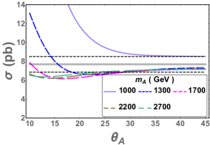
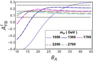
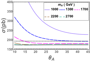
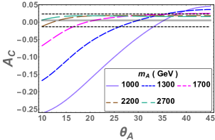
We calculate the differential cross-section of the process ($pp$)$p\bar{p}\to t\bar{t}\to l\nu b\bar{t}$ at the Tevatron with $\sqrt{s}=1.96$ TeV and at the LHC with $\sqrt{s}=7$ TeV and $\sqrt{s}=13$ TeV for the SM + bSM with CTEQ6l CTEQ6l1:Pumplin2002 parton distribution functions with factorization scale fixed at $Q=2m_{t}=345$ GeV, the top quark mass is taken to be $m_{t}=172.5$ TeV and $\alpha_{s}\left(m_{t}\right)=0.108$.

The cross-section calculated for the Tevatron, LHC and the AC and AFB of the $t\overline{t}$ at those experiments in the axigluon model are shown in figure 1. We constrain the model parameter space by limiting the predicted observables $\sigma_{p\overline{p}\to t\overline{t}}$, $\sigma_{pp\to t\overline{t}}$, $A_{FB}$ and $A_{C}$ to within $2\sigma$ of the experimental values. As the values of $\theta_{A}$ and $m_{A}$ grow larger, the couplings reduce, the mass of the mediating particle rises and the bSM contributions to the observables reduce. At large values of $\theta_{A}$, the figures correspond to an axigluon model with only an axial coupling with the top quark and no resulting top polarization. For a lower mass range, constraints from the LHC allow only larger $\theta_{A}$ and hence smaller coupling values, at the same time, interference with SM gives a constraint at the Tevatron which allows some region in the large coupling range as well. $A_{C}$ gives a complimentary constraint and rules out large values of $\theta_{A}$ (couplings close to $g_{s}$) for a smaller mass of the axigluon. The result is that for the low masses of the axigluon, a range of couplings corresponding to $\theta_{A}\sim(25\textdegree-35\textdegree)$ and masses $m_{A}\sim(1300-1900)$ GeV are allowed. Masses above these values are allowed for almost all parameter space with the only constraints coming from the Tevatron cross-section.

CMS results constrain the mass of an additional massive spin-1 colour octet of particles (eg. Kaluza Klein-gluon) which couple to gluons and quarks to above $3.5$ TeV, which excludes the parameter region favoured by the experimental results from the $t\overline{t}$ process mentioned above Khachatryan:2015sja . The constraints can be evaded if the assumption of equal couplings of axigluons to light quarks and the top quark is relaxed. In this case, the values of coupling $g_{V},g_{A}$ we use can be split into $g_{V}^{q},g_{A}^{q}$ and $g_{V}^{t},g_{A}^{t}$ where, the couplings with quarks would be constrained strongly from the axigluon direct production bounds. In the limit that the vector and axial couplings are equal or any one of the vector or axial coupling is small, our results can be recast into the modified model by using $g_{v/a}^{2}=g_{v/a}^{q}g_{v/a}^{t}$. A more generalized version of such an axigluon model has already been discussed in the literature Aguilar-Saavedra:2014nja along with constraints on the model from lepton and top quark asymmetries at the Tevatron and the LHC.

The axigluon model can be constrained from B physics Chivukula:2010Axnotallowed results however, given the somewhat large hadronic uncertainties in some of the variables along with the possibility of relaxing these constraints in various modified axigluon models and/or by constructing UV completions, for the purpose of this study, we do not take these constraints into account.

IV U-channel scalar exchange model

In a second class of bSM models, AFB is explained due to contributions of a $t$- or $u$-channel exchange of new particles between the top quark-antiquark pair. The corresponding mediators do not show resonance behaviour and are elusive in the bump-hunting type analyses in $t\overline{t}$ pair production though they do contribute significantly to the angular distributions. We consider here a scalar particle called diquark, which, similar to a squark with R parity violation, transforms as a triplet under $SU(3)_{c}$ and has a charge of $-\frac{4}{3}$. The corresponding coupling is given by the lagrangian below,

$$\mathcal{L} = \overline{t^{c}}T^{a}(y_{s}+y_{p}\gamma^{5})u\phi_{a}+h.c.$$ (5)

$$t^{c} = -i\gamma^{2}t^{*}$$ (6)

$$= -i(\overline{t}\gamma^{0}\gamma^{2})^{T}$$

We assume a right-handed coupling of the scalar with the up type quarks with $y=y_{s}=y_{p}$. This ensures that flavour constraints and proton stability bounds are avoided. The density matrices for top pair production in the diquark model are given in Appendix B.2. All calculations in this work are performed at tree level. The NLO contributions become important to study the effects on invariant mass distributions which we have not included here. These calculations are under progress for both axigluon and diquark models.

IV.1 Constraints on the coloured scalar model

(a) Cross-section at the Tevatron with $\sqrt{s}=1.96$ TeV

(b) AFB at the Tevatron with $\sqrt{s}=1.96$ TeV

(c) Cross-section at the LHC with $\sqrt{s}=7$ TeV

(d) $A_{C}$ at the LHC with $\sqrt{s}=7$ TeV

Figure 2: Observables at the top-quark level at the Tevatron and the LHC (7 TeV) as a function of the Yukawa coupling for various values of the diquark masses. The experimentally measured values are marked in grey and the respective 2$\sigma$ errors in dotted black lines. The line spacing changes from solid to a dashed line with wider spaces as mass values rise from 100-2600 GeV. .

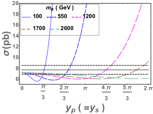
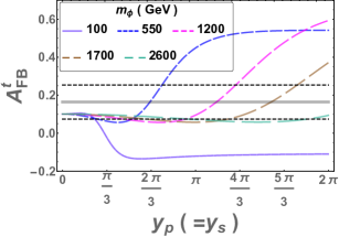
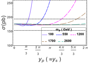
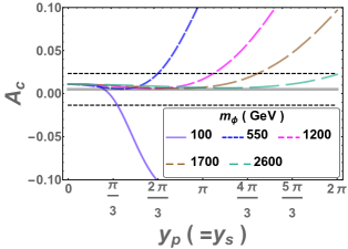
As in the case of an $s$-channel resonance in the previous section, the constraints are obtained from the measurements of the top pair production cross-section at the Tevatron and the LHC (7 TeV), the AFB and AC. We explore a parameter space of $m_{\phi}\in[100,3000]$ GeV and $y\in[0,\,2\pi]$ chosen so as to explore all the values of the coupling within the perturbative limit. As the value of the coupling rises, contribution of the bSM to all the observables becomes larger. For lighter diquarks, negative values of AFB and AC are predicted for large values of the coupling, though this mass range is ruled out by independent constraints from diquark pair production CMS:2013gqa . In figure 2 we can notice from the top left panel that, as in the case of the axigluon, the Tevatron cross-section provides the constraints in the parameter space of lower masses and couplings. In the next panel, the AFB measured at the Tevatron disallows lighter scalars and also constraints a part of coupling values for larger masses. The LHC cross-section constraints large coupling regions which give larger contribution and the cut-off coupling increases as mass of the scalar becomes heavier. The AC also allows larger coupling parameter space for higher masses of the scalar.

The constraints from pair production of the coloured scalar from gluon fusion at the LHC are weak (~300 GeV) as reinterpreted from corresponding constraints on squarks Chatrchyan:2013izb . There are further constraints on lower mass scalars from atomic parity violation Gresham:2012wc . Constraints from $uu\to tt$ can be avoided by adding flavour symmetries (see for example Grinstein:2011yv ).

V Constraints from dijet production at LHC

(a) Constraints on axigluon parameter space

(b) Constraints on diquark parameter space

Figure 3: Allowed parameter space for axigluon and diquark models are depicted as Green (lighter) coloured regions. Figure 3a shows the constraints from dijet searches as the blue (darker) shaded area. In figure 3b the dotted line represents the bound from pair production of bSM particles at LHC.

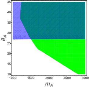
The coloured scalar and vector bSM models get constrained from searches for direct production of bSM particles and subsequent decay to di-jet and four jet final states ( $q\bar{q}\to A\to 2j$ , $gg\to\phi\phi^{\dagger}\to 4j$). Earlier constraints on axigluon model were obtained from searches of narrow resonances from dijet spectrum at 8 TeV LHC and were extended to the case of a wider width axigluon model with $\frac{\Gamma_{A}}{m_{A}}=0.3$ where the axigluon has only axial-vector couplings Diaz:2013tfa (also see Choudhury:2011cg for bSM particle off-shell effects in dijet searches). We reinterpret these constraints to the case of the axigluon model in this study which has both axial-vector and vector couplings with the quarks and find the excluded parameter range where $\frac{\Gamma_{A}}{m_{A}}<0.3$. Figure 3a shows the parameter space allowed for the axigluon model. The following constraints are put on the model parameters to obtain the allowed values : reinterpreted searches for bSM resonances in dijet production, $t\bar{t}$ cross-section and top charge asymmetry measurements at 7 TeV LHC and cross-section, top forward backward asymmetry measurements at the Tevatron as discussed in section III.1. The coupling values corresponding to $\theta_{A}>27^{\circ}$ are ruled out for axigluon masses up to $\sim 4$ TeVs as these narrow, resonant particles would have been detected in the dijet searches. The allowed values of couplings correspond to $\theta_{A}\sim 10^{\circ}-27^{\circ}$ for the mass range between 1.5 TeV to 3 TeV. Note that the constraints from dijet searches may be relaxed if the magnitude of coupling of axigluon is different for the third generation of quarks as compared to the first and the second generations.

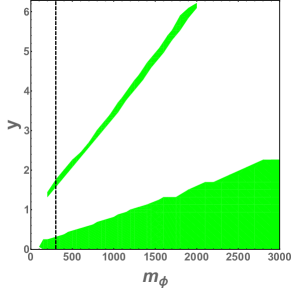
The diquark mass is bound from below to $m_{\phi}>\sim 300$ GeV from pair production of diquarks via gluon fusion at the LHC Chatrchyan:2013izb . The direct production bounds along with the constraints obtained from top quark pair production cross-section and top charge, forward backward asymmetry measurements at LHC and Tevatron (see section IV) are shown in figure 3b. A narrow strip of parameter space is allowed when couplings are large due to destructive interference effects. Besides this region, the rest of the allowed diquark parameter space follows the expected behaviour of small coupling values $<0.2$ for lower masses and for a diquark of mass 3 TeV, $y_{s}$ as large as 2 is allowed.

VI Polarization of the top quark and decay-lepton distributions

The decay kinematics of leptons embeds the information regarding top quark production dynamics, kinematics and polarization Papaefstathiou:2011kd . Different lepton observables embed these effects in different ways and so provide a number of probes which are all correlated with the top quark kinematics and polarization. For a detailed analysis of top quark decay see Jezabek:1988topdecayleptondist ; Godbole:2006ldistandtpol . In this section we discuss distributions of the lepton polar angle, azimuthal angle and energy in SM decay of top quark and construct asymmetries based on these distributions to probe top quark bSM interactions.

A proper treatment of the decay distributions of the top quark requires the spin density matrix formulation, which preserves correlations between the spin states in the production and in the decay.

The spin density matrix for $t$ in the production of a $t\overline{t}$ pair with the spin of $\overline{t}$ summed over, can be expressed as

$$\rho_{t\overline{t}\,production}\left(\lambda_{t},\lambda_{t}^{\prime}\right)=\sum_{\lambda_{\bar{t}}}\mathcal{M}_{production}\left(\lambda_{t},\lambda_{\bar{t}}\right)\mathcal{M}_{production}^{\star}\left(\lambda_{t}^{\prime},\lambda_{\bar{t}}\right)$$ (7)

The density matrix gets SM contributions $\rho_{SM}^{gg}\left(\lambda_{t},\lambda_{t}^{\prime}\right)$ and $\rho_{SM}^{q\bar{q}}\left(\lambda_{t},\lambda_{t}^{\prime}\right)$ respectively from gluon-gluon and quark-anti-quark initial states, a contribution $\rho_{bSM}\left(\lambda_{t},\lambda_{t}^{\prime}\right)$ from the bSM model, and a contribution $\rho_{interference}\left(\lambda_{t},\lambda_{t}^{\prime}\right)$ from the interference between the SM amplitude and the bSM amplitude:

$$\rho\left(\lambda_{t},\lambda_{t}^{\prime}\right)=\rho_{SM}^{gg}\left(\lambda_{t},\lambda_{t}^{\prime}\right)+\rho_{SM}^{q\overline{q}}\left(\lambda_{t},\lambda_{t}^{\prime}\right)+\rho_{bSM}\left(\lambda_{t},\lambda_{t}^{\prime}\right)+\rho_{Interference}\left(\lambda_{t},\lambda_{t}^{\prime}\right)$$ (8)

The spin density matrix for the decay of the top quark is given by

$$\Gamma_{top\,decay}\left(\lambda_{t},\lambda_{t}^{\prime}\right)=\mathcal{M}_{decay}\left(\lambda_{t}\right)\mathcal{M}_{decay}^{\star}\left(\lambda_{t}^{\prime}\right),$$ (9)

with the spins of the decay products summed over.

The squared amplitude for the combined process of production and decay is given by

$$\overline{|\mathcal{M}|^{2}} = \frac{\pi\delta\left(p_{t}^{2}-m_{t}^{2}\right)}{\Gamma_{t}m_{t}}\sum_{\lambda_{t},\lambda_{t}^{\prime}}\rho\left(\lambda_{t},\lambda_{t}^{\prime}\right)\Gamma\left(\lambda_{t},\lambda_{t}^{\prime}\right)$$ (10)

This expression assumes a narrow-width approximation for the top quark. Top decay is assumed to progress through SM processes. In the rest frame of top quark, the differential decay distribution of the top quark is given by

$$\frac{d\Gamma_{t}}{\Gamma d\cos(\theta)}=\frac{1+A_{p}k_{f}\cos\theta}{2}$$ (11)

where $\theta$ is the angle between top-quark spin direction and the momentum of the decay product $f$. For $N(\lambda_{t})$ number of top quarks with helicity $\lambda_{t}$, polarization $A_{p}$ is defined as,

$$A_{P}=\frac{N(\lambda_{t}=+)-N(\lambda_{t}=-)}{N(\lambda_{t}=+)+N(\lambda_{t}=-)},$$ (12)

and the coefficient $k_{f}$ is called the top-spin analysing power of the decay particle $f$. For the case of leptons as the final state particles, the factor $k_{f}=1$ at tree level in the SM. When the top quark is boosted in the direction of its spin quantization axis, eqn (11) gets modified to

$$\frac{\mbox{d}\Gamma^{Boosted}}{\Gamma\mbox{d}\cos(\theta_{tl})}=\frac{\left(1-\beta^{2}\right)(1+\lambda_{t}\cos\theta_{tl}-\beta(\cos\theta_{tl}+\lambda_{t}))}{2(1-\beta\cos\theta_{tl})^{3}},$$ (13)

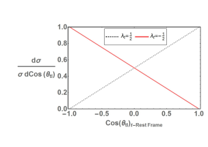
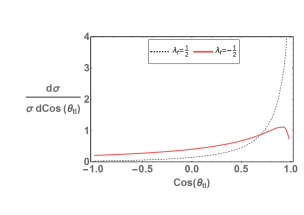
where $\theta_{tl}$ is defined as the angle between lepton and top quark momenta in the boosted frame. Lepton kinematic distributions for the tree-level SM differential cross-section for the process $p\overline{p}\to t\overline{t}\to l+jets$ with $\sqrt{s}=1.96$ TeV are presented in the figure 4. The energy and azimuthal lepton distributions are uncorrelated with the polarization in the rest frame of the top quark, though correlate with the polarization in the boosted frame. Higher-order corrections to the production and decay processes have been calculated for the SM and the distributions are found to be qualitatively unchanged Melnikov:2009dn ; Bernreuther:2014dla . Due to this reason, we expect that the effect of higher-order corrections to the asymmetries constructed from decay-lepton distributions to be relatively small as the corrections partially cancel out within the difference and ratio taken to derive the asymmetry.

(a) Lepton polar angle distribution in top quark rest frame.

(b) Lepton polar angle distribution in the lab frame.

(c) Lepton Azimuthal angle distribution in the lab frame

(d) Lepton energy distribution in the lab frame

Figure 4: The tree-level lepton polar and azimuthal distributions for $p\overline{p}\to t\overline{t}\to l+jets$ with $\sqrt{s}=1.96$ TeV. In the above plots, the average boost of the $t\bar{t}$ pairs is 0.34.

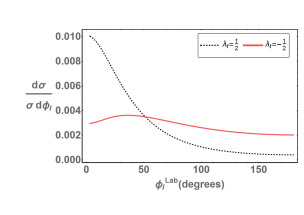
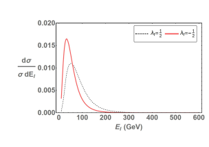
A lepton polar-angle asymmetry with respect to the top-quark direction can be defined by

$$A_{FB}^{tl} = \frac{\sigma(\cos(\theta_{tl})>0)-\sigma(\cos(\theta_{tl})<0)}{\sigma(\cos(\theta_{tl})>0)+\sigma(\cos(\theta_{tl})<0)}$$ (14)

$A_{FB}^{tl}$ has been measured at both LHC and Tevatron in the lab and $t\bar{t}$ center of momentum frame, albeit with large statistical errors and different results from CDF and D0 cdf_Alpm . Integrating eqn (11) the top rest-frame lepton asymmetry can be related to the polarization of the top quark,

$$A_{P}=\mbox{$\frac{1}{2}A_{FB}^{tl,t-rest}$}.$$ (15)

In QCD, $A_{FB}^{tl,rest}=A_{p}=0$, though in the boosted frame, the lepton polar asymmetry with respect to the top quark is large even in a tree-level SM calculation.

In the lab frame where the top quarks and leptons are boosted and the cross-section convoluted with the pdf, the correlations between various angles and energies become more complicated. The lepton polar angle with respect to the proton beam is a convenient observable which does not require top-quark rest frame or momenta reconstruction. The lepton polar asymmetry $A_{FB}^{l}$ in the lab frame is also 0 at tree level in SM QCD. $A_{FB}^{l}$ is identically 0 at the LHC due to the symmetric nature of the initial state. This asymmetry according to our analysis correlates the best with the off-diagonal elements of the top quark density matrix for the $l+jets$ process considered (see Section VIII) for both axigluon and diquark models. An analytic study of the lepton polar angle and its correlation with top AFB and polarization has also been made by Berger et al. Berger:2012_assym_corr . They relate the lepton and the top quark level polar asymmetries and subsequently use this relation to distinguish between a sequential axigluon and a W’ type model Berger2013_AlandPol .

In the top-quark rest frame, other lepton kinematic variables : azimuthal angle and its energy have no dependence on the helicity of the top quark and hence the integrated asymmetries are uncorrelated with the polarization. It has been noted in the literature that the lepton azimuthal distributions correlate with the polarization of the top quark in a boosted frame Godbole:2006ldistandtpol ; Godbole:2010phidist_tpol_LHC ; Godbole:2011_AlAphiAp ; Barger:2011philcorr . Sums and differences of azimuthal decay angle in top pair production process have also been used in the literature to study the polarization and spin correlations of top quark in detail Baumgart:2012ay . For a detailed analysis of analytic relation between polarization of a heavy particle and decay particle azimuthal asymmetry, see Boudjema:2009fz . We reproduce the azimuthal distribution in the lab frame for the SM $t\overline{t}$ pair production process at the Tevatron in figure 4c. The azimuthal distribution can be measured at both Tevatron and LHC and requires only partial reconstruction of top quark rest frame. The azimuthal angle is defined by assuming that the top quark lies in the x-z plane with proton (beam) direction as z-axis. From this distribution, an azimuthal asymmetry about a point $\phi_{0}$ can be defined as

$$A_{\phi}^{l} = \frac{\sigma(\pi>\phi_{l}>\phi_{0})-\sigma(\phi_{l}<\phi_{0})}{\sigma(\pi>\phi_{l}>\phi_{0})+\sigma(\phi_{l}<\phi_{0})}$$ (16)

A natural choice for the value of $\phi_{0}$ would be the point of intersection of the distributions corresponding to left and right helicity top quarks. For SM, this point is about $\phi=50\textdegree$ for both Tevatron and the LHC. The SM point would correspond to 0 polarization and would maximize correlation with bSM contribution. We assume a value of $\phi_{0}$ a bit lower at $40\textdegree$. Since the positive helicity top quark have larger differential cross-section in this region, this choice enhances correlations of the lepton level asymmetry for larger positive (or smaller negative) values of polarization. The standard model tree-level results for this asymmetry at the Tevatron and the LHC respectively are given in table 4 . In the lab frame, due to the boost and rotation from the direction of the top quark, $A_{\phi}$ is sensitive to both the polarization and the parity breaking or t-channel structure of the top quark coupling.

Asymmetry	Q = $m_{t}$	Q = $2m_{t}$
$A_{FB}^{tl}$	$0.645$	$0.642$
$A_{\phi}^{l}$	$-0.113$	$-0.116$
$A_{E_{l}}^{l}$	$0.381$	$0.397$

(a) Tevatron $\sqrt{s}=1.96$ TeV

Asymmetry	Q = $m_{t}$	Q = $2m_{t}$
$A_{FB}^{tl}$	$0.748$	$0.748$
$A_{\phi}^{l}$	$-0.075$	$-0.077$
$A_{E_{l}}^{l}$	$0.138$	$0.146$

(b) LHC $\sqrt{s}=7$ TeV

Asymmetry	Q = $m_{t}$	Q = $2m_{t}$
$A_{FB}^{tl}$	$0.789$	$0.788$
$A_{\phi}^{l}$	$-0.041$	$-0.044$
$A_{E_{l}}^{l}$	$0.036$	$0.038$

(c) LHC $\sqrt{s}=13$ TeV

Table 4: Scale dependence of SM values of various asymmetries tree level.

Another observable which can be constructed from the decay-lepton kinematics is the lepton energy asymmetry about a chosen energy $E_{0}$:

$$A_{E_{l}}^{l}=\frac{\sigma(E_{l}>E_{0})-\sigma(E_{l}<E_{0})}{\sigma(E_{l}>E_{0})+\sigma(E_{l}<E_{0})}$$ (17)

No reconstruction of the top-quark rest frame is needed to measure $E_{l}$. Just like the azimuthal case, this asymmetry can be measured both at the LHC and the Tevatron. The lepton energy distribution is sensitive to the polarization of top quark Godbole:2006ldistandtpol , as shown in figure 4d. Similar asymmetries based on the energy of decay particles or the ratios of these energies have been used in the literature to study bSM physics Shelton:2008topPol ; Godbole:2011_AlAphiAp ; Carmona:2014gra ; Prasath:2014mfa . We define the lepton energy asymmetry about a value of $E_{0}=80$ GeV, to act as a better discriminator between bSM and SM. Ideally, the point of intersection of the positive and the negative top-polarization curves should form the best correlation with the top polarization, though this point varies with the energy and the invariant mass of the initial state. Standard model values of asymmetries mentioned in this section are given in table 4. It would be interesting to use SM distributions at NLO to decide the reference points $E_{0},\phi_{0}$, but since in the end we construct asymmetries, we expect that the qualitative behaviour of our results would not change.

In the recent past, polarization measurements have been made by collaborations both at the Tevatron and the LHC. The polarization at the Tevatron points towards a small positive value and that at the LHC to small negative values. This is consistent with the small coupling and large mass regimes of both the models studied here.

In the next section, we use correlations among top charge and forward-backward asymmetries, decay lepton angular and energy asymmetries, and polarization to uncover specific properties of bSM particles which can be inferred from the Tevatron and the LHC data.

VII Correlations

The parameter space of $m_{A}\in[1000,3000]$ GeV and $\theta_{A}\in[10,45]$ are explored for the axigluon model and $m_{\phi}\in[100,3000]$ GeV and $y_{s}\in[0,2\pi]$ for the coloured scalar. The figures in the section VII.2 show parameter space allowed by the constraints mentioned in sections III, IV.

VII.1 Correlations between charge and forward-backward asymmetries

The correlation between the AC at 7 TeV LHC and the AFB at the Tevatron have been used in the literature constrain various bSM models(see for example DC:2010_W'z'Axdiq ). These constraints are model dependent and the asymmetries are not in general tightly correlated Drobnak:2012cz . We show similar correlations in figure 5 where we plot $A_{C}$ vs $A_{FB}$, using the relation

$$A_{C/FB}=A_{C/FB}^{SM\_NLO}+A_{C/FB}^{bSM}$$ (18)

This relation is valid as long as the bSM physics corrects the SM cross-section of the $t\overline{t}$ pair production process by a small amount.

(a) The red markers represent axigluon model with only axial interactions($g_{V}=0,g_{A}^{t}=g_{s}$). The size of the plus marks represent a mass range from 1000-3000 GeV

(b) diquark model with right handed couplings to u,t quarks. The size of the plus marks represent a mass range from 100-3000 GeV

Figure 5: Correlation between top-quark asymmetries $A_{FB}^{t}$ vs $A_{C}^{t}$ at the Tevatron and the LHC ($\sqrt{s}=7$TeV). The grey solid and dashed lines represent the observed values of the respective asymmetries and their $2\sigma$ errors.

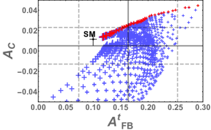
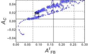
The pure axial axigluon which leads to unpolarized top quark is disfavoured as it does not have a parameter space where it can explain both $A_{FB}$ and $A_{C}$ experimental values. In the diquark model, the coupling to right handed quarks is sampled from 0 to $2\pi$ where large mass or small couplings lead to a better agreement with SM NLO values of asymmetries.

VII.2 Correlations among lepton and top asymmetries

In this section, we study the correlations among top polarization, top asymmetries and decay lepton asymmetries. We show that combined, they form sensitive discriminators between models with different dynamics. The top-quark and decay-lepton asymmetries are calculated at various points in the parameter space allowed by the experimental constraints discussed in section III and IV. The expected polarization of the top quark, for corresponding points in the parameter space, is represented in colour contrast form inside the graphs and clear trends for the polarization can be observed. In all the following figures, top-quark asymmetries represented on the $x$-axis are calculated as shown in eqn (18) and the lepton asymmetries shown on the $y$-axis are calculated including SM+bSM contributions at tree level.

VII.2.1 Asymmetry correlations for the Tevatron

(a) Lepton polar asymmetry Tevatron $\sqrt{s}=1.96$ TeV.

(b) Lepton polar asymmetry Tevatron $\sqrt{s}=1.96$ TeV.

Figure 6: Correlations between top AFB and lab frame $\theta_{l},\theta_{tl}$ asymmetries at the Tevatron $\sqrt{s}=1.96$ TeV

(a) Lepton Azimuthal asymmetry about $\phi_{0}$ for the Tevatron $\sqrt{s}=1.96$ TeV.

(b) Lepton energy asymmetry about energy $E_{0}$ for the Tevatron $\sqrt{s}=1.96$ TeV.

Figure 7: Correlations between top AFB and the lepton energy and azimuthal asymmetries at the Tevatron $\sqrt{s}=1.96$ TeV

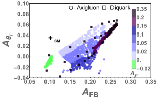
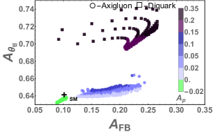
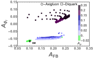
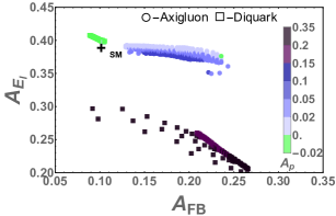
The correlations of the lepton-level asymmetries with the top AFB at the Tevatron are shown in figures 6a, 6b, 7a and 7b. For the case of axigluon as its mass is increased, the polarization rises until $m_{A}\sim 1650$ GeV and then drops again for even larger masses. The diquark model predicts negative polarization for a significant portion of parameter space, turning positive only for large couplings. The large mass region for the diquark also favours large (negative) values of azimuthal asymmetry, smaller lepton polar asymmetry and larger lepton energy asymmetry. Lepton polar asymmetry correlation with top AFB shows large overlap between the two models. The observed value for the lab-frame lepton polar asymmetry in tables 2,3 points towards a positive polarization between $A_{\theta_{l}}=0.2\mbox{ to }1.1$. In this region (see figure 6a), a large positive value for polarization is favoured for the diquark model and a large contribution to top AFB. The axigluon model is compatible with both the observed value of $A_{\theta_{l}}$ and a small contribution towards longitudinal polarization for a significant part of its parameter space. Figure 6b shows the asymmetry in the lepton polar angle with respect the top direction, $A_{\theta_{tl}}$, which is equal to twice the top polarization, eqn (15), when calculated in top-quark rest frame. It receives contribution from bSM physics via the boost of the parent top quark. In the lab frame, large deviations of $A_{\theta_{tl}}$ from the SM value correlate with large contribution to the top-quark polarization from the bSM. The values of asymmetries grow closer to the corresponding SM values with increase in mass and reduction in the bSM coupling strength. The azimuthal asymmetry and lepton polar asymmetry with respect to the top-momentum direction ($A_{\theta_{tl}}$) and lepton energy asymmetry in figures 6b, 7a and 7b discriminate well between the $s$-channel and $u$-channel exchange models though the parameter spaces within the model are clumped together. When combined with polarization, all correlations enhance their discriminating power especially to distinguish between $s$-channel and $u$-channel models as they predict opposite signs of polarization for a large portion of parameter space.

VII.2.2 Asymmetry correlations for the LHC

(a) Lepton Azimuthal asymmetry about $\phi_{0}=40$ degrees for the LHC $\sqrt{s}=7$ TeV

(b) Lepton polar asymmetry(w.r.t top quark direction) for the LHC $\sqrt{s}=7$ TeV

(c) Lepton Energy asymmetry about $E_{0}=80$ GeV for the LHC $\sqrt{s}=7$ TeV

Figure 8: Correlations between lepton and top kinematic asymmetries at the LHC-7 TeV.

(a) Lepton Azimuthal asymmetry about $\phi_{0}=40$ degrees for the LHC $\sqrt{s}=13$ TeV

(b) Lepton polar asymmetry(w.r.t top quark direction) for the LHC $\sqrt{s}=13$ TeV

(c) Lepton Energy asymmetry about $E_{0}=80$ GeV for the LHC $\sqrt{s}=13$ TeV

Figure 9: Correlations between lepton and top kinematic asymmetries at the LHC-13 TeV.

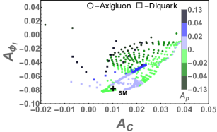
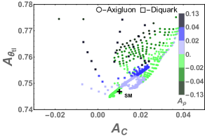
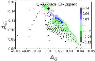
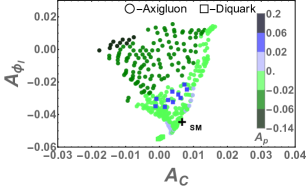
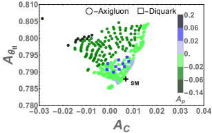
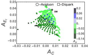
The lepton-level asymmetry correlations with $t\overline{t}$ charge asymmetry are shown in figures 8a-8c for the LHC $7$ TeV run and figures 9a-9c for the LHC $13$ TeV. The plots are made for the region of the model parameter space constrained in sections III and IV. For the $\sqrt{s}=7$ TeV calculation, we use $m_{t}=172.5$ GeV and factorization scale $Q=2m_{t}$ and $\alpha_{s}=0.108$ to remain consistent with the ATLAS and CMS reconstruction of $A_{C}$. For $\sqrt{s}=13$ TeV, , the mass of top quark is chosen at the updated central value $m_{t}=173.2GeV$ and $Q=2m_{t}$ with $\alpha_{s}=0.108$ and CTEQ6l pdf.

A large portion of the parameter space predicts a negative polarization at 7 TeV LHC for the axigluon model. The diquark model predicts a small negative polarization for small couplings with quarks. When heavier diquark models are considered, larger couplings are allowed leading to a large positive contribution to the polarization. Observed values of polarization from CMS and ATLAS are compatible with $-0.03<A_{p}<0.07$, which covers a large region of parameter space for both axigluon and diquark models. As in the case of the Tevatron, polarization is an important discriminant between models for the LHC as well, especially when combined with decay-lepton asymmetries. It is able to distinguish overlapping parameter space regions between the two models. This is more true when the couplings are small and the bSM effects are more difficult to detect as the $s$-channel and $u$-channel exchanges predict small polarization, but with opposite signs in this region. The energy asymmetry becomes smaller for the LHC at 13 TeV due to the effect of the overall boost. The values of azimuthal and polar asymmetries do not change significantly for higher energy and so remain good observables for the study of top quark dynamics.

VIII Asymmetry correlations and top transverse polarization

As remarked earlier, keeping full spin correlations between the production and decay of the top quark in a coherent manner requires the spin density matrix formalism. In this formalism, the top polarization, which played a significant role in the above analysis, corresponds to the difference in the diagonal elements of the density matrix, as seen from eqn (12). The off-diagonal elements of the density matrix can also be significant in practice, and they would contribute to the transverse polarization of the top quark, corresponding to a spin quantization axis transverse to the momentum. In SM, these terms arise at loop level and have been studied in the literature along-with transverse polarization and observables have been suggested to measure their contribution Bernreuther:1995cx . We examine in this section what role these off-diagonal matrix elements and transverse top polarization play in the two models considered in this study.

Following the formalism developed in Godbole:2006ldistandtpol , the spin density matrix integrated over a suitable final-state phase space can be written as $\sigma(\lambda,\lambda^{\prime})=\sigma_{tot}\mathcal{P}_{t}(\lambda,\lambda^{\prime})$, where $\sigma_{tot}$ represents the unpolarized cross section. The matrix $\mathcal{P}_{t}(\lambda,\lambda^{\prime})$ can be written as

$$\mathcal{P}_{t}(\lambda,\lambda^{\prime})=\left(\begin{array}[]{cc}1+\eta_{3}&\eta_{1}-i\eta_{2}\\ \eta_{1}+i\eta_{2}&1-\eta_{3}\end{array}\right).$$ (19)

Here $\eta_{3}$ is the longitudinal polarization, $\eta_{1}$ and $\eta_{2}$ are polarizations along two transverse directions. The expressions for the $\eta_{i}$ in terms of the top-quark density matrix $\sigma\left(\lambda_{t},\lambda_{t}^{{}^{\prime}}\right)$ can be written as,

$$\eta_{3} = \frac{\left(\sigma\left(++\right)-\sigma\left(--\right)\right)}{\sigma_{tot}}$$ (20)

$$\eta_{1} = \frac{\left(\sigma\left(+-\right)+\sigma\left(-+\right)\right)}{\sigma_{tot}}$$ (21)

$$i\eta_{2} = \frac{\left(\sigma\left(+-\right)-\sigma\left(-+\right)\right)}{\sigma_{tot}}$$ (22)

Splitting the top density matrix as shown in eqn (10) under the narrow-width approximation, the helicity-dependent decay density matrix in the rest frame of top quark separates into a simple functions of the decay angle:

$$d\Gamma(\lambda,\lambda^{\prime})=c\times A(\lambda,\lambda^{\prime})d\Omega_{l}$$ (23)

where

$$A=\begin{array}[]{c|cc}\lambda\downarrow,\lambda^{\prime}\to&+&-\\ \hline\cr+&1+\cos\left(\theta_{l}\right)&\sin\left(\theta_{l}\right)e^{i\phi_{l}}\\ -&\sin\left(\theta_{l}\right)e^{-i\phi_{l}}&1-\cos\left(\theta_{l}\right).\end{array}$$ (24)

$\Omega_{l}$ is the solid angle in which the lepton is emitted and $c$ is the integrated contribution of the rest of the decay kinematic variables. The resulting lepton angular distribution in the lab frame is ,

$$\frac{d\sigma}{d\cos\left(\theta_{l}\right)d\phi_{l}}=c\sigma_{tot}\left(1+\eta_{3}\cos\left(\theta_{l}\right)+\eta_{1}\sin\left(\theta_{l}\right)\cos\left(\phi_{l}\right)+\eta_{2}\sin\left(\theta_{l}\right)\sin\left(\phi_{l}\right)\right)$$ (25)

The off-diagonal elements in the top-quark production density matrix do not contribute to the total cross-section due to an overall factor of $\sin\left(\theta_{l}\right)$ which integrates to 0. They do contribute instead to the kinematic distributions of the decay particle, although this effect is quite small for most observables.

In this study, we find that the lepton polar angle asymmetry defined in the lab frame is sensitive to the off-diagonal terms in the top quark density matrix eqn (7). The transverse polarization originating from these off-diagonal terms contains further information about the dynamics of top-quark interaction. This relation has been pointed out before in the context of a wide-width colour octet bSM particle Aguilar-Saavedra:2014yea ; Baumgart:2013yra .

In figure 10 we study the contribution of off-diagonal terms to the lepton distributions and present the distributions for a few sample masses of bSM particles.

(a) axigluon

(b) diquark

Figure 10: Contribution to Lepton asymmetry from the off-diagonal terms of top density matrix calculated in the lab frame for the Tevatron $\sqrt{s}=1.96$ TeV for the axigluon and diquark models. The red lines represent the asymmetry for diagonal density matrix and the black line represents the distribution for the case of total density matrix. The darker lines represent allowed regions of parameter space.

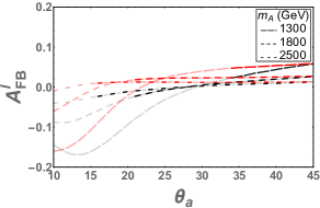
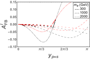
It can be seen that the contribution of the off-diagonal density matrix elements can be significant, and is particularly important for the diquark model. These can in turn lead to significant transverse polarization of the top for appropriate range of parameters which could be measured experimentally.

IX Conclusions

The forward backward asymmetry of the top quark in top-pair production process at the Tevatron collider was, for a long time, anomalously large and a persistent effect observed independently by both D0 and CDF detectors. It has been demonstrated only relatively recently that NNLO contributions give rise to an $A_{FB}^{t}$ of the right order of magnitude and seems to be in agreement with the values measured experimentally. Previously, many bSM models had been proposed with parity breaking interactions to explain the observed $A_{FB}^{t}$. Many of these models predicted a charge asymmetry at the LHC. Since LHC has a gluon dominated initial state as opposed to the Tevatron where $q\bar{q}$ was the primary initial state, the asymmetries predicted for LHC coming from the bSM couplings to the quarks get diluted. The data gives values for $A_{C}$ consistent with the SM and so far there has been no evidence for the new particles predicted in the different bSM models. Under these circumstances there is a need to construct measures which can distinguish between different sources of the $A_{FB}^{t}$: either SM or bSM.

One such measure is provided by polarization of the top quark which has a non-zero value in the presence of a parity breaking interaction. Within SM, top polarization is close to 0. Observables that correlate with top polarization can be used to distinguish between various SM and bSM contributions. In continuation to a previous work where correlations between polarization and forward backward asymmetry were used to constraint bSM DC:2010_W'z'Axdiq , we have introduced the correlations between lepton polar, azimuthal and energy asymmetries and top charge asymmetry and showed how they can be used together with top longitudinal polarization to distinguish between SM and bSM.

In the reference Krohn:2011tw the authors have constructed dilepton central charge and azimuthal asymmetries and studied it along with top quark polarization, forward backward asymmetry and $t\bar{t}$ spin correlations for benchmark models of G’ and W’. Subsequently, in reference Berger:2012_assym_corr the authors have shown that the lepton polar asymmetry and top forward backward asymmetry and lepton charge asymmetry vs top charge asymmetry correlations can be useful in the study of W’ and G’ models. Our work adds multiple new observables to the analysis of new physics in $t\bar{t}$ pair production which include single-lepton azimuthal angle, energy and polar angle (wrt top quark) in the lab frame which show signatures from parity breaking in top interactions and help isolate and constrain the interactions of bSM particles.

We demonstrate the efficacy of the correlations between forward backward asymmetry and the lepton asymmetries at Tevatron and charge asymmetry and lepton angluar,energy asymmetries at LHC, by utilizing a representative s-channel model, axigluon and an u-channel model, diquark. Constraints on these models are obtained based on measured values of $t\bar{t}$ cross-section at Tevatron and LHC 7TeV, $A_{FB}^{t}$ and $A_{C}^{t}$ and resonance searches in dijet, four jet cross sections. The parameter space of axigluon allowed within 2-$\sigma$ of the measured values of the stated observables includes a lower bound on the mass of axigluon at 1.5 TeV with a corresponding coupling $\theta_{A}>27^{\circ}$. The allowed mass of the diquark is bounded from below by 300 GeV and masses above are allowed with the coupling of the model bounded from above by a value of 0.2 for smaller masses which rises to $y_{s}<2$ corresponding to $m_{\phi}=3$ TeV. Another sliver of parameter space is allowed for larger couplings of the diquark due to destructive interference effects.

For the first time we have presented the complete density matrix of the top quark, including the off-diagonal elements for top quark pair production process, in the axigluon and diquark models to aid further studies. We use these to show that the lepton polar asymmetry in the lab frame shows a correlation with the transverse polarization of the top quark for axigluon model and even more significantly for the diquark model. The lepton asymmetry usually considered in studies of top polarization is calculated from lepton polar angle with respect to the top quark and it does not show this correlation with transverse polarization. The correlation of transverse polarization with lepton azimuthal or energy asymmetry is also very small.

Finally, we extend our analysis to 13 TeV LHC where, even though the values of the asymmetries get diluted, the correlations between accurate measurements of charge asymmetry and lepton asymmetries still separate out bSM and the SM in the 2 dimensional space. Taken together, these correlations can indeed be used to improve significance of the constraints on bSM from LHC data even in the initial stages of low luminosity.

Appendix A AC at $13$ TeV LHC

Since the AC calculated at NLO for 13TeV LHC was unavailable at the time of submission of this work, we note that the available charge asymmetry values SM_LHC_Ac form a smooth function of the beam energy and fit them to a polynomial to find the AC as a function of the beam energy. We obtain a fit to a polynomial presented in eqn (26) with goodness of fit parameter $r^{2}=0.9995$.

$$Ac\left(\sqrt{s}\right)=3.12\times 10^{-2}-4.37\times 10^{-3}\sqrt{s}+2.6269\times 10^{-4}s-5.683\times 10^{-6}s^{\frac{3}{2}}$$ (26)

This gives a value of Ac(13 TeV)=0.0063.

Appendix B $t\overline{t}$ Production density matrices

B.1 axigluon density matrices

With $C_{\theta}=\cos(\theta_{t})$, $S_{\theta}=\sin(\theta_{t})$, $\beta=\sqrt{1-\frac{4m_{t}^{2}}{\hat{s}}}$ and $\beta_{A}=\sqrt{1-\frac{4m_{t}^{2}}{m_{A}^{2}}}$.

$$\rho_{bSM}^{++} = \frac{1}{\Gamma_{A}{}^{2}m_{A}{}^{2}+\left(m_{A}{}^{2}-\hat{s}\right){}^{2}}\hat{s}^{2}\{\frac{1}{18}(g_{A}{}^{2}+g_{V}{}^{2})(6g_{\text{At}}g_{V}\beta+3g_{\text{At}}{}^{2}\beta^{2}-g_{V}{}^{2}\left(-4+\beta^{2}\right))$$ (27)

$$+\frac{4}{9}g_{A}g_{V}\left(g_{V}+g_{\text{A}}^{t}\beta\right){}^{2}C_{\theta}+\frac{1}{18}\left(g_{A}{}^{2}+g_{V}{}^{2}\right)\beta\left(2g_{\text{A}}^{t}g_{V}+g_{\text{A}}^{t}{}^{2}\beta+g_{V}{}^{2}\beta\right)C_{2\theta}\}$$

$$\rho_{bSM}^{+-} = \frac{1}{\Gamma_{A}{}^{2}m_{A}{}^{2}+\left(m_{A}{}^{2}-\hat{s}\right){}^{2}}\hat{s}^{2}\left(-\frac{8g_{A}g_{V}{}^{3}m_{t}S_{\theta}}{9\sqrt{\hat{s}}}-\frac{4g_{\text{A}}^{t}g_{V}\left(g_{A}{}^{2}+g_{V}{}^{2}\right)m_{t}\beta C_{\theta}S_{\theta}}{9\sqrt{\hat{s}}}\right)$$ (28)

$$\rho_{bSM}^{-+} = (\rho_{bSM}^{+-})^{\star}$$ (29)

$$\rho_{bSM}^{--} = \frac{1}{\Gamma_{A}{}^{2}m_{A}{}^{2}+\left(m_{A}{}^{2}-\hat{s}\right){}^{2}}\hat{s}^{2}\{\frac{1}{18}(g_{A}{}^{2}+g_{V}{}^{2})(-6g_{\text{A}}^{t}g_{V}\beta+3g_{\text{A}}^{t}{}^{2}\beta^{2}-g_{V}{}^{2}\left(-4+\beta^{2}\right))$$

$$-\frac{4}{9}g_{A}g_{V}\left(g_{V}-g_{\text{A}}\beta\right){}^{2}C_{\theta}+\frac{1}{18}\left(g_{A}{}^{2}+g_{V}{}^{2}\right)\beta\left(-2g_{\text{A}}^{t}g_{V}+g_{\text{A}}^{t}{}^{2}\beta+g_{V}{}^{2}\beta\right)C_{2\theta}\}$$

$$\rho_{Interference}^{++} = \frac{g_{s}^{2}}{9\left(\Gamma_{A}{}^{2}m_{A}{}^{2}+\left(m_{A}{}^{2}-\hat{s}\right){}^{2}\right)}\hat{s}\left(-m_{A}{}^{2}+\hat{s}\right)$$

$$\times\left(4g_{A}\left(g_{V}+g_{\text{A}}^{t}\beta\right)C_{\theta}+g_{V}\left(4g_{v}+3g_{\text{A}}^{t}\beta-g_{V}\beta^{2}+\beta\left(g_{\text{A}}^{t}+g_{V}\beta\right)C_{2\theta}\right)\right)$$

$$\rho_{Interference}^{+-} = \frac{g_{s}^{2}}{9\left(\Gamma_{A}{}^{2}m_{A}{}^{2}+\left(m_{A}{}^{2}-\hat{s}\right){}^{2}\right)}4m_{t}\sqrt{\hat{s}}S_{\theta}$$ (32)

$$\times\left(g_{A}\left(2g_{v}\left(m_{A}{}^{2}-\hat{s}\right)+ig_{\text{At}}\Gamma_{A}m_{A}\beta\right)+g_{\text{A}}^{t}g_{V}\left(m_{A}{}^{2}-\hat{s}\right)\beta C_{\theta}\right)$$

$$\rho_{Interference}^{-+} = (\rho_{Interference}^{+-})^{\star}$$ (33)

$$\rho_{Interference}^{--} = \frac{g_{s}^{2}}{9\left(\Gamma_{A}{}^{2}m_{A}{}^{2}+\left(m_{A}{}^{2}-\hat{s}\right){}^{2}\right)}\left(m_{A}{}^{2}-\hat{s}\right)\hat{s}$$

$$\times\left(4g_{A}\left(g_{V}-g_{\text{A}}^{t}\beta\right)C_{\theta}+g_{V}\left(3g_{\text{A}}^{t}\beta+g_{V}\left(\beta^{2}-4\right)+\beta\left(g_{\text{A}}^{t}-g_{V}\beta\right)C_{2\theta}\right)\right)$$

To present the dependence on top boost and polar angle clearly the amplitude square is written in terms of the polar angle $\theta$ in $t\overline{t}$ center of momentum frame. The off-diagonal terms in the gluon initiated process are zero and the diagonal terms in gluon initiated process are not dependent on the top quark polarization therefore we have omitted these here and they can be found in many references including DC:2010_W'z'Axdiq . Decay width of axigluon at tree level is given by,

$$\Gamma_{A} = \frac{4\pi}{6m_{A}}\{g_{A}^{2}\left(m_{A}^{2}\left(\beta_{A}+5\right)-4m_{t}^{2}\beta_{A}\right)+g_{V}^{2}\left(m_{A}^{2}\left(\beta_{A}+5\right)+2m_{t}^{2}\beta_{A}\right)\}$$ (35)

B.2 diquark density matrices

The top-quark spin density matrix for the $u$-channel exchange is given below in $t\overline{t}$ center of momentum frame. The notation and SM only contributions remain the same as for the case of the $s$-channel model.

$$\rho_{bSM}^{++} = \frac{2\hat{s}\left(y_{P}^{2}+y_{S}^{2}\right)}{48\left(\beta\hat{s}C_{\theta}-2m_{t}^{2}+2m_{\phi}^{2}+\hat{s}\right){}^{2}}\times$$ (36)

$$\{\hat{s}\left(2y_{P}y_{S}\left(\beta+\beta C_{\theta}^{2}+2C_{\theta}\right)+(y_{P}^{2}+y_{S}^{2})\left(2\beta C_{\theta}+C_{\theta}^{2}+1\right)\right)$$

$$-4C_{\theta}m_{t}^{2}\left(C_{\theta}\left(y_{P}^{2}+y_{S}^{2}\right)+2y_{P}y_{S}\right)\}$$

$$\rho_{bSM}^{+-} = -\frac{\hat{s}^{3/2}m_{t}y_{P}y_{S}\left(\beta C_{\theta}+1\right)\left(y_{P}^{2}+y_{S}^{2}\right)S_{\theta}}{6\left(\beta\hat{s}C_{\theta}-2m_{t}^{2}+2m_{\phi}^{2}+\hat{s}\right){}^{2}}$$ (37)

$$\rho_{bSM}^{-+} = (\rho_{bSM}^{+-})^{\star}$$ (38)

$$\rho_{bSM}^{--} = \frac{\hat{s}\left(y_{P}^{2}+y_{S}^{2}\right)}{24\left(\beta\hat{s}C_{\theta}-2m_{t}^{2}+2m_{\phi}^{2}+\hat{s}\right){}^{2}}$$ (39)

$$\{\hat{s}\left(-2y_{P}y_{S}\left(\beta+\beta C_{\theta}^{2}+2C_{\theta}\right)+(y_{P}^{2}+y_{S}^{2})\left(2\beta C_{\theta}+C_{\theta}^{2}+1\right)\right)$$

$$-4C_{\theta}m_{t}^{2}\left(C_{\theta}\left(y_{P}^{2}+y_{S}^{2}\right)-2y_{P}y_{S}\right)\}$$

$$\rho_{Interference}^{++} = \frac{g_{s}^{2}}{18\left(\beta\hat{s}C_{\theta}-2m_{t}^{2}+2m_{\phi}^{2}+\hat{s}\right)}\times\{4\left(C_{\theta}^{2}-1\right)m_{t}^{2}\left(y_{P}^{2}+y_{S}^{2}\right)$$ (40)

$$-\hat{s}\left(2y_{P}y_{S}\left(\beta+\beta C_{\theta}^{2}+2C_{\theta}\right)+(y_{P}^{2}+y_{S}^{2})\left(2\beta C_{\theta}+C_{\theta}^{2}+1\right)\right)\}$$

$$\rho_{Interference}^{+-} = \frac{g_{s}^{2}2\sqrt{\hat{s}}m_{t}y_{P}S_{\theta}y_{S}\left(\beta C_{\theta}+2\right)}{9\left(\beta\hat{s}C_{\theta}-2m_{t}^{2}+2m_{\phi}^{2}+\hat{s}\right)}$$

$$\rho_{Interference}^{-+} = (\rho_{Interference}^{+-})^{\star}$$ (41)

$$\rho_{Interference}^{--} = \frac{g_{s}^{2}}{18\left(\beta\hat{s}C_{\theta}-2m_{t}^{2}+2m_{\phi}^{2}+\hat{s}\right)}\times\{4\left(C_{\theta}^{2}-1\right)m_{t}^{2}\left(y_{P}^{2}+y_{S}^{2}\right)$$

$$-\hat{s}\left(-2y_{P}y_{S}\left(\beta+\beta C_{\theta}^{2}+2C_{\theta}\right)+(y_{P}^{2}+y_{S}^{2})\left(2\beta C_{\theta}+C_{\theta}^{2}+1\right)\right)\}$$

References

- (1) BaBar Collaboration, J. Lees et al., “Evidence of decays with hadronic B tags,” Phys.Rev. D88 no. 3, (2013) 031102, arXiv:1207.0698 [hep-ex].
- (2) CMS Collaboration, “Search for Lepton Flavour Violating Decays of the Higgs Boson,”. CMS-PAS-HIG-14-005.
- (3) D0 Collaboration, V. M. Abazov et al., “Measurement of the Forward-Backward Asymmetry in the Production of Mesons in Collisions at = 1.96 TeV,” Phys. Rev. Lett. 114 (2015) 051803, arXiv:1411.3021 [hep-ex].
- (4) SLD Electroweak Group, DELPHI, ALEPH, SLD, SLD Heavy Flavour Group, OPAL, LEP Electroweak Working Group, L3 Collaboration, S. Schael et al., “Precision electroweak measurements on the resonance,” Phys. Rept. 427 (2006) 257–454, arXiv:hep-ex/0509008 [hep-ex].
- (5) C. W. Murphy, “Bottom-Quark Forward-Backward and Charge Asymmetries at Hadron Colliders,” arXiv:1504.02493 [hep-ph].
- (6) D0 Collaboration, V. Abazov et al., “First measurement of the forward-backward charge asymmetry in top quark pair production,” Phys.Rev.Lett. 100 (2008) 142002, arXiv:0712.0851.
- (7) CDF Collaboration, T. Aaltonen et al., “Forward-backward asymmetry in top quark production in collisions at tev,” Phys.Rev.Lett. 101 (2008) 202001, arXiv:0806.2472.
- (8) D0 Collaboration, V. M. Abazov et al., “Measurement of the forward-backward asymmetry in top quark-antiquark production in ppbar collisions using the lepton+jets channel,” Phys.Rev. D90 no. 7, (2014) 072011, arXiv:1405.0421 [hep-ex].
- (9) N. Kidonakis, “Top quark forward-backward asymmetry at approximate ,” Phys.Rev. D91 no. 7, (2015) 071502, arXiv:1501.01581 [hep-ph].
- (10) D. Choudhury, R. M. Godbole, R. K. Singh, and K. Wagh, “Top production at the tevatron/lhc and nonstandard, strongly interacting spin one particles,” Phys.Lett. B657 (2007) 69–76, arXiv:0705.1499.
- (11) O. Antunano, J. H. Kuhn, and G. Rodrigo, “Top quarks, axigluons and charge asymmetries at hadron colliders,” Phys.Rev. D77 (2008) 014003, arXiv:0709.1652 [hep-ph].
- (12) P. Ferrario and G. Rodrigo, “Constraining heavy colored resonances from top-antitop quark events,” Phys.Rev. D80 (2009) 051701, arXiv:0906.5541.
- (13) P. H. Frampton, J. Shu, and K. Wang, “axigluon as possible explanation for forward-backward asymmetry,” Phys.Lett. B683 (2010) 294–297, arXiv:0911.2955.
- (14) D. Choudhury, R. M. Godbole, S. D. Rindani, and P. Saha, “Top polarization, forward-backward asymmetry and new physics,” Phys.Rev. D84 (2011) 014023, arXiv:1012.4750.
- (15) S. Dutta, A. Goyal, and M. Kumar, “Top quark physics in the vector color-octet model,” Phys.Rev. D87 no. 9, (2013) 094016, arXiv:1209.3636 [hep-ph].
- (16) S. Fajfer, J. F. Kamenik, and B. Melic, “Discerning New Physics in Top-Antitop Production using Top Spin Observables at Hadron Colliders,” JHEP 1208 (2012) 114, arXiv:1205.0264 [hep-ph].
- (17) J. A. Aguilar-Saavedra and M. Perez-Victoria, “Simple models for the top asymmetry: Constraints and predictions,” JHEP 09 (2011) 097, arXiv:1107.0841 [hep-ph].
- (18) M. Gresham, J. Shelton, and K. M. Zurek, “Open windows for a light axigluon explanation of the top forward-backward asymmetry,” JHEP 1303 (2013) 008, arXiv:1212.1718 [hep-ph].
- (19) S. Jung, H. Murayama, A. Pierce, and J. D. Wells, “Top quark forward-backward asymmetry from new t-channel physics,” Phys.Rev. D81 (2010) 015004, arXiv:0907.4112.
- (20) A. Papaefstathiou and K. Sakurai, “Determining the Helicity Structure of Third Generation Resonances,” JHEP 1206 (2012) 069, arXiv:1112.3956 [hep-ph].
- (21) J. Shu, T. M. Tait, and K. Wang, “Explorations of the top quark forward-backward asymmetry at the tevatron,” Phys.Rev. D81 (2010) 034012, arXiv:0911.3237.
- (22) V. Barger, W.-Y. Keung, and C.-T. Yu, “Tevatron asymmetry of tops in a w’,z’ model,” Phys.Lett. B698 (2011) 243–250, arXiv:1102.0279.
- (23) A. Rajaraman, Z. Surujon, and T. M. Tait, “Asymmetric Leptons for Asymmetric Tops,” arXiv:1104.0947 [hep-ph].
- (24) K. M. Patel and P. Sharma, “Forward-backward asymmetry in top quark production from light colored scalars in SO(10) model,” JHEP 1104 (2011) 085, arXiv:1102.4736 [hep-ph].
- (25) E. L. Berger, Z. Sullivan, and H. Zhang, “LHC and Tevatron constraints on a W’ model interpretation of the top quark forward-backward asymmetry,” Phys. Rev. D88 no. 11, (2013) 114026, arXiv:1309.7110 [hep-ph].
- (26) D.-W. Jung, P. Ko, J. S. Lee, and S.-h. Nam, “Model independent analysis of the forward-backward asymmetry of top quark production at the tevatron,” Phys.Lett. B691 (2010) 238–242, arXiv:0912.1105.
- (27) D. Buarque Franzosi and C. Zhang, “Probing the top-quark chromomagnetic dipole moment at next-to-leading order in QCD,” Phys.Rev. D91 no. 11, (2015) 114010, arXiv:1503.08841 [hep-ph].
- (28) S. S. Biswal, S. Mitra, R. Santos, P. Sharma, R. K. Singh, et al., “New physics contributions to the forward-backward asymmetry at the Tevatron,” Phys.Rev. D86 (2012) 014016, arXiv:1201.3668 [hep-ph].
- (29) J. Shu, K. Wang, and G. Zhu, “A Revisit to Top Quark Forward-Backward Asymmetry,” Phys.Rev. D85 (2012) 034008, arXiv:1104.0083 [hep-ph].
- (30) S. Westhoff, “Top Charge Asymmetry – Theory Status Fall 2013,” arXiv:1311.1127 [hep-ph].
- (31) M. Jezabek and J. H. Kuhn, “Lepton spectra from heavy quark decay,” Nucl.Phys. B320 (1989) 20.
- (32) R. M. Godbole, S. D. Rindani, and R. K. Singh, “Lepton distribution as a probe of new physics in production and decay of the t quark and its polarization,” JHEP 0612 (2006) 021, arXiv:hep-ph/0605100.
- (33) W. Bernreuther and Z.-G. Si, “Distributions and correlations for top quark pair production and decay at the Tevatron and LHC.,” Nucl.Phys. B837 (2010) 90–121, arXiv:1003.3926 [hep-ph].
- (34) J. Aguilar-Saavedra, W. Bernreuther, and Z. Si, “Collider-independent top quark forward-backward asymmetries: standard model predictions,” Phys.Rev. D86 (2012) 115020, arXiv:1209.6352 [hep-ph].
- (35) W. Bernreuther and Z.-G. Si, “Top quark and leptonic charge asymmetries for the Tevatron and LHC,” Phys.Rev. D86 (2012) 034026, arXiv:1205.6580 [hep-ph].
- (36) J. Aguilar-Saavedra and R. Herrero-Hahn, “Model-independent measurement of the top quark polarisation,” Phys.Lett. B718 (2013) 983–987, arXiv:1208.6006 [hep-ph].
- (37) J. L. Hewett, J. Shelton, M. Spannowsky, T. M. P. Tait, and M. Takeuchi, “ Meets LHC,” Phys. Rev. D84 (2011) 054005, arXiv:1103.4618 [hep-ph].
- (38) CDF, D0 Collaboration, T. A. Aaltonen et al., “Combination of measurements of the top-quark pair production cross section from the Tevatron Collider,” Phys.Rev. D89 no. 7, (2014) 072001, arXiv:1309.7570 [hep-ex].
- (39) CMS Collaboration, “Combination of ATLAS and CMS top-quark pair cross section measurements using proton-proton collisions at sqrt(s) = 7 TeV,”. CMS-PAS-TOP-12-003.
- (40) ATLAS Collaboration, “Combination of ATLAS and CMS top-quark pair cross section measurements using up to 1.1 fb-1 of data at 7 TeV,”. ATLAS-CONF-2012-134 ETC.
- (41) N. Kidonakis and R. Vogt, “The theoretical top quark cross section at the tevatron and the lhc,” Phys.Rev. D78 (2008) 074005, arXiv:0805.3844.
- (42) M. Czakon and A. Mitov, “Top++: A Program for the Calculation of the Top-Pair Cross-Section at Hadron Colliders,” Comput.Phys.Commun. 185 (2014) 2930, arXiv:1112.5675 [hep-ph].
- (43) M. Czakon, P. Fiedler, and A. Mitov, “Total Top-Quark Pair-Production Cross-Section at Hadron Colliders Through ,” Phys.Rev.Lett. 110 (2013) 252004, arXiv:1303.6254 [hep-ph].
- (44) V. Ahrens, A. Ferroglia, M. Neubert, B. D. Pecjak, and L. L. Yang, “The top-pair forward-backward asymmetry beyond nlo,” Phys.Rev. D84 (2011) 074004, arXiv:1106.6051.
- (45) CDF Collaboration, T. Aaltonen et al., “Measurement of the top quark forward-backward production asymmetry and its dependence on event kinematic properties,” Phys.Rev. D87 (2013) 092002, arXiv:1211.1003.
- (46) M. Czakon, P. Fiedler, and A. Mitov, “Resolving the Tevatron top quark forward-backward asymmetry puzzle,” arXiv:1411.3007 [hep-ph].
- (47) ATLAS, CMS Collaboration, “Combination of ATLAS and CMS charge asymmetry measurements using LHC proton-proton collisions at TeV,”. ATLAS-CONF-2014-012 ETC.
- (48) J. H. Kuhn and G. Rodrigo, “Charge asymmetries of top quarks at hadron colliders revisited,” JHEP 1201 (2012) 063, arXiv:1109.6830.
- (49) CDF Collaboration, T. A. Aaltonen et al., “Measurement of the leptonic asymmetry in ttbar events produced in ppbar collisions at tev,” Phys.Rev. D88 (2013) 072003, arXiv:1308.1120.
- (50) D0 Collaboration, V. M. Abazov et al., “Measurement of the forward-backward asymmetry in the distribution of leptons in events in the leptonjets channel,” Phys.Rev. D90 no. 7, (2014) 072001, arXiv:1403.1294 [hep-ex].
- (51) CDF Collaboration, T. Aaltonen et al., “Measurement of Spin Correlation in Collisions Using the CDF II Detector at the Tevatron,” Phys.Rev. D83 (2011) 031104, arXiv:1012.3093 [hep-ex].
- (52) D0 Collaboration, Y. Peters, “ Spin Correlations at D0,” PoS ICHEP2012 (2013) 236, arXiv:1210.7189 [hep-ex].
- (53) ATLAS Collaboration, G. Aad et al., “Measurements of spin correlation in top-antitop quark events from proton-proton collisions at TeV using the ATLAS detector,” Phys.Rev. D90 no. 11, (2014) 112016, arXiv:1407.4314 [hep-ex].
- (54) CMS Collaboration, S. Chatrchyan et al., “Measurements of spin correlations and top-quark polarization using dilepton final states in collisions at = 7 TeV,” Phys.Rev.Lett. 112 no. 18, (2014) 182001, arXiv:1311.3924 [hep-ex].
- (55) S. Frixione and B. R. Webber, “Matching NLO QCD computations and parton shower simulations,” JHEP 0206 (2002) 029, arXiv:hep-ph/0204244 [hep-ph].
- (56) ATLAS Collaboration, G. Aad et al., “Measurement of Top Quark Polarization in Top-Antitop Events from Proton-Proton Collisions at = 7TeV Using the ATLAS Detector,” Phys.Rev.Lett. 111 no. 23, (2013) 232002, arXiv:1307.6511 [hep-ex].
- (57) P. H. Frampton and S. L. Glashow, “Chiral color: An alternative to the standard model,” Phys.Lett. B190 (1987) 157.
- (58) P. Frampton, “Chiral dilepton model and the flavor question,” Phys.Rev.Lett. 69 (1992) 2889–2891.
- (59) J. Pumplin, D. Stump, J. Huston, H. Lai, P. M. Nadolsky, et al., “New generation of parton distributions with uncertainties from global qcd analysis,” JHEP 0207 (2002) 012, arXiv:hep-ph/0201195.
- (60) CMS Collaboration, V. Khachatryan et al., “Search for resonances and quantum black holes using dijet mass spectra in proton-proton collisions at 8 TeV,” Phys.Rev. D91 no. 5, (2015) 052009, arXiv:1501.04198 [hep-ex].
- (61) J. Aguilar-Saavedra, “Portrait of a colour octet,” JHEP 1408 (2014) 172, arXiv:1405.5826 [hep-ph].
- (62) R. S. Chivukula, E. H. Simmons, and C.-P. Yuan, “axigluons cannot explain the observed top quark forward-backward asymmetry,” Phys.Rev. D82 (2010) 094009, arXiv:1007.0260.
- (63) CMS Collaboration, C. Collaboration, “Search for pair production of resonances decaying to a top quark plus a jet in final states with two leptons,”.
- (64) CMS Collaboration, S. Chatrchyan et al., “Search for pair-produced dijet resonances in four-jet final states in pp collisions at = 7 TeV,” Phys.Rev.Lett. 110 (2013) 141802, arXiv:1302.0531 [hep-ex].
- (65) M. I. Gresham, I.-W. Kim, S. Tulin, and K. M. Zurek, “Confronting Top AFB with Parity Violation Constraints,” Phys.Rev. D86 (2012) 034029, arXiv:1203.1320 [hep-ph].
- (66) B. Grinstein, A. L. Kagan, M. Trott, and J. Zupan, “Forward-backward asymmetry in production from flavour symmetries,” Phys.Rev.Lett. 107 (2011) 012002, arXiv:1102.3374 [hep-ph].
- (67) B. Diaz and A. R. Zerwekh, “axigluon Phenomenology using ATLAS dijet data,” Int.J.Mod.Phys. A28 (2013) 1350133, arXiv:1308.0166 [hep-ph].
- (68) D. Choudhury, R. M. Godbole, and P. Saha, “Dijet resonances, widths and all that,” JHEP 01 (2012) 155, arXiv:1111.1054 [hep-ph].
- (69) K. Melnikov and M. Schulze, “NLO QCD corrections to top quark pair production and decay at hadron colliders,” JHEP 0908 (2009) 049, arXiv:0907.3090 [hep-ph].
- (70) W. Bernreuther, P. González, and C. Mellein, “Decays of polarized top quarks to lepton, neutrino and jets at NLO QCD,” Eur.Phys.J. C74 no. 3, (2014) 2815, arXiv:1401.5930 [hep-ph].
- (71) E. L. Berger, Q.-H. Cao, C.-R. Chen, and H. Zhang, “Interpretations and implications of the top quark rapidity asymmetries and ,” Phys.Rev. D88 (2013) 014033, arXiv:1209.4899.
- (72) E. L. Berger, Q.-H. Cao, J.-H. Yu, and H. Zhang, “Measuring top-quark polarization in top-pair + missing energy events,” arXiv:1305.7266.
- (73) R. M. Godbole, K. Rao, S. D. Rindani, and R. K. Singh, “On measurement of top polarization as a probe of production mechanisms at the lhc,” JHEP 1011 (2010) 144, arXiv:1010.1458.
- (74) R. M. Godbole, L. Hartgring, I. Niessen, and C. D. White, “Top polarisation studies in and production,” JHEP 1201 (2012) 011, arXiv:1111.0759.
- (75) V. Barger, W.-Y. Keung, and B. Yencho, “Azimuthal correlations in top pair decays and the effects of new heavy scalars,” Phys.Rev. D85 (2012) 034016, arXiv:1112.5173.
- (76) M. Baumgart and B. Tweedie, “A New Twist on Top Quark Spin Correlations,” JHEP 1303 (2013) 117, arXiv:1212.4888 [hep-ph].
- (77) F. Boudjema and R. K. Singh, “A Model independent spin analysis of fundamental particles using azimuthal asymmetries,” JHEP 0907 (2009) 028, arXiv:0903.4705 [hep-ph].
- (78) J. Shelton, “Polarized tops from new physics: signals and observables,” Phys.Rev. D79 (2009) 014032, arXiv:0811.0569.
- (79) A. Carmona, M. Chala, A. Falkowski, S. Khatibi, M. M. Najafabadi, et al., “From Tevatron’s top and lepton-based asymmetries to the LHC,” JHEP 1407 (2014) 005, arXiv:1401.2443 [hep-ph].
- (80) A. Prasath, R. M. Godbole, and S. D. Rindani, “Top polarisation measurement and anomalous coupling,” arXiv:1405.1264 [hep-ph].
- (81) J. Drobnak, J. F. Kamenik, and J. Zupan, “Flipping t tbar Asymmetries at the Tevatron and the LHC,” Phys.Rev. D86 (2012) 054022, arXiv:1205.4721 [hep-ph].
- (82) W. Bernreuther, A. Brandenburg, and P. Uwer, “Transverse polarization of top quark pairs at the Tevatron and the large hadron collider,” Phys.Lett. B368 (1996) 153–162, arXiv:hep-ph/9510300 [hep-ph].
- (83) J. Aguilar-Saavedra, “Quantum coherence, top transverse polarisation and the Tevatron asymmetry ,” Phys.Lett. B736 (2014) 132–136, arXiv:1405.1412 [hep-ph].
- (84) M. Baumgart and B. Tweedie, “Transverse Top Quark Polarization and the ttbar Forward-Backward Asymmetry,” JHEP 1308 (2013) 072, arXiv:1303.1200 [hep-ph].
- (85) D. Krohn, T. Liu, J. Shelton, and L.-T. Wang, “A Polarized View of the Top Asymmetry,” Phys. Rev. D84 (2011) 074034, arXiv:1105.3743 [hep-ph].