NLO QCD corrections to off-shell top–antitop production with leptonic decays in association with a Higgs boson at the LHC
Abstract
We compute the hadronic production of top–antitop pairs in association with a Higgs boson at next-to-leading-order QCD, including the decay of the top and antitop quark into bottom quarks and leptons. Our computation is based on full leading and next-to-leading-order matrix elements for and includes all non-resonant contributions, off-shell effects and interferences. Numerical results for the integrated cross section and several differential distributions are given for the LHC operating at 13 TeV using a fixed and a dynamical factorization and renormalization scale. The use of the dynamical instead of the fixed scale improves the perturbative stability in high-energy tails of most distributions, while the integrated cross section is hardly affected differing by only about one per cent and leading to almost the same factor of about 1.17.
1 Introduction
After the discovery of a new boson of a mass around 125 GeV by the CMS and ATLAS Collaborations Aad:2012tfa ; Chatrchyan:2012ufa at the LHC, the determination of its quantum numbers and couplings to other particles has become a high priority in particle physics. Results from the first run of the LHC strongly support the hypothesis that this particle is the Higgs boson predicted by the Standard Model (SM) of particle physics. In the Brout–Englert–Higgs symmetry breaking mechanism of the SM the Higgs boson is the key for understanding the origin of mass. Since in this framework the Higgs boson couples to fermions with a strength proportional to their mass via Yukawa interactions, its coupling to the heaviest quark, the top quark, is of particular interest. The main production mechanism of the Higgs boson in the SM is gluon fusion, . This process is sensitive to the top-quark Yukawa coupling, but possible heavy particles beyond the SM running in the loop bias its determination. On the other hand, the production of a SM Higgs boson in association with a top-quark pair allows a direct access of the top-quark Yukawa coupling already at tree level, disentangling it from possible beyond-SM contributions.
Leading-order (LO) predictions for production for stable Higgs boson and top quarks have been presented in Refs. Raitio:1978pt ; Ng:1983jm ; Kunszt:1984ri ; Gunion:1991kg ; Marciano:1991qq . Since LO predictions of QCD processes suffer from large perturbative uncertainties higher-order corrections have to be taken into account for adequate theoretical predictions. The cross section for production at next-to-leading-order (NLO) QCD is known for more than 10 years Beenakker:2001rj ; Beenakker:2002nc ; Reina:2001sf ; Dawson:2002tg ; Dawson:2003zu . Meanwhile, NLO QCD corrections have been matched to parton showers Frederix:2011zi ; Garzelli:2011vp ; Hartanto:2015uka and recently electroweak corrections to production have been computed Frixione:2014qaa ; Yu:2014cka ; Frixione:2015zaa . NLO QCD corrections for the important background processes and production have been worked out in Refs. Bredenstein:2008zb ; Bredenstein:2009aj ; Bevilacqua:2009zn ; Bredenstein:2010rs and Refs. Bevilacqua:2010ve ; Bevilacqua:2011aa ; Bevilacqua:2014qfa , respectively, and matched to parton showers in Refs. Kardos:2013vxa ; Cascioli:2013era ; Garzelli:2014aba and Ref. Hoeche:2014qda .
Several searches for the associated production of the Higgs boson with a top-quark pair for a variety of decay channels have been published by ATLAS ATLAS:2012cpa ; ATLAS:2014 ; Aad:2014lma ; ATLAS-CONF-2015-006 ; Aad:2015gra and CMS CMS:2012qaa ; CMS:2013sea ; CMS-PAS-HIG-13-015 ; Chatrchyan:2013yea ; Khachatryan:2014qaa ; Khachatryan:2015ila . These searches are challenging due to a large background from and production, and so far no evidence of a signal over background has been found. The current ratio of the measured signal cross section to the SM expectation quoted by ATLAS is Aad:2015gra and by CMS Khachatryan:2015ila for a Higgs-boson mass of 125 GeV.
In this article we present the calculation of the NLO QCD corrections to the hadronic production of a positron, a muon, missing energy, two b jets and a SM Higgs boson, which we assume to be stable () at the 13 TeV LHC, which includes the resonant production of a top–antitop-quark pair in association with a Higgs boson with a subsequent leptonic decay of the top and the antitop quark. Our calculation includes all NLO QCD correction effects in production and top decays and also takes into account all off-shell, non-resonant and interference effects of the top quarks. We consider the fixed renormalization and factorization scale used in Ref. Beenakker:2002nc and alternatively the dynamical scale choice from Ref. Frederix:2011zi and investigate their quality in reducing the dependence of the integrated cross section as well as differential distributions on the factorization and renormalization scales. The phase-space integration is performed with a newly implemented in-house multi-channel Monte Carlo program, using phase-space mappings similar to Ref. Dittmaier:2002ap . The Monte Carlo implements the dipole subtraction method Catani:1996vz ; Dittmaier:1999mb ; Catani:2002hc ; Phaf:2001gc for the computation of the real corrections and is linked to the matrix-element generator Recola Actis:2012qn for the computation of the LO and NLO matrix elements as well as colour- and spin-correlated squared matrix elements needed for the evaluation of subtraction terms.
The calculation follows in many respects the one of in Ref. Denner:2012yc . In particular, since the additional Higgs boson in the final state has no colour charge, the contributing Catani–Seymour dipoles Catani:1996vz ; Catani:2002hc are the same. For the hadronic process we find a qualitative similar behaviour of NLO corrections to the integrated cross section as well as for differential distributions of the same observables. Where appropriate we compare results and point out differences. Moreover, we compare our results for the total cross sections to those of existing calculations for on-shell Higgs boson and top quarks Beenakker:2002nc ; Frederix:2011zi .
The paper is organised as follows. In Section 2 we discuss details of the calculation such as contributing subprocesses and Feynman diagrams and explain some technical aspects of the real (Section 2.1) and virtual (Section 2.2) corrections. We present numerical results for the LHC operating at in Section 3. In Section 3.1 we list and explain the input parameters, jet definition, cuts and scale choices for our calculation, while results for integrated cross sections and a discussion of the scale dependence are provided in Section 3.2. In Section 3.4 we display and discuss several differential distributions for a fixed and a dynamical scale choice. We have performed several checks of our calculation which we present in Section 4. Our conclusions are given in Section 5.
2 Details of the calculation
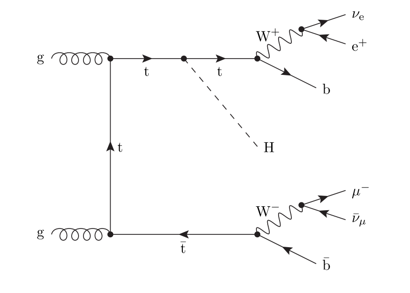
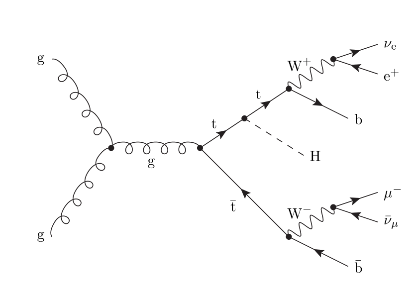

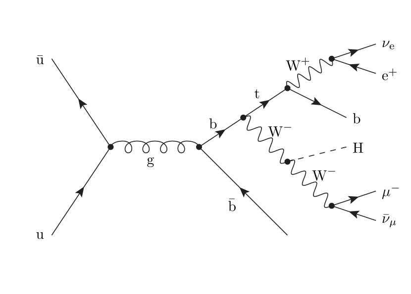
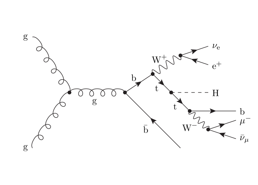
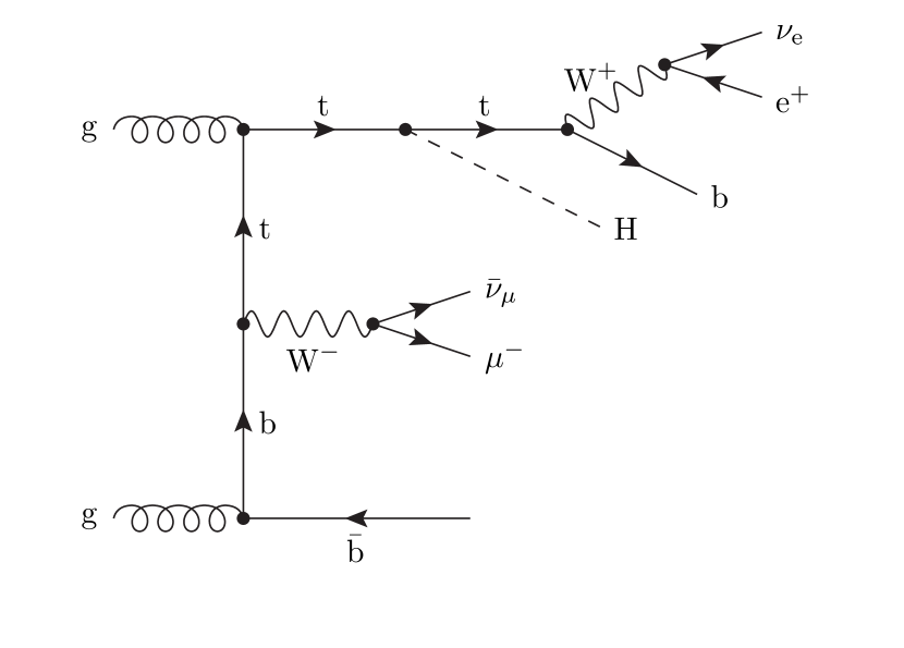
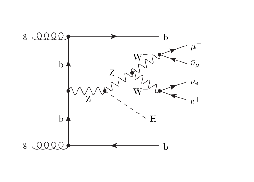
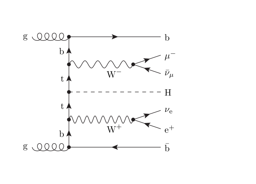
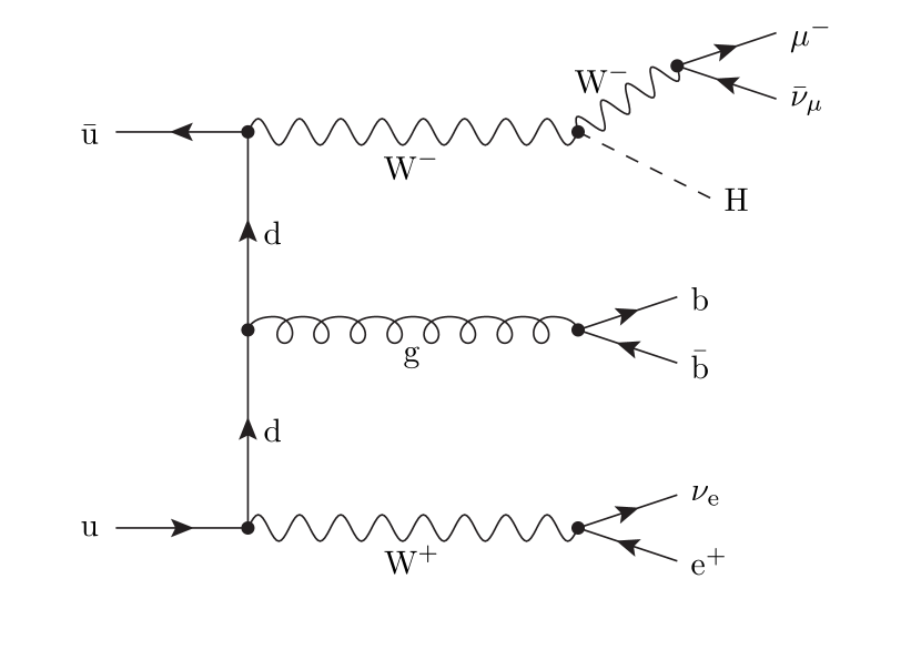
We compute the QCD corrections to the full hadronic process
| (1) |
We consider the tree-level amplitude at including all resonant, non-resonant, and off-shell effects of the top quarks and all interferences. Neglecting flavour mixing as well as contributions from the suppressed bottom-quark parton densities and counting u, d, c and s quarks separately, we distinguish 5 partonic channels for the LO hadronic process: the gluon-induced process and four processes from by substituting different quark flavours (). Throughout this paper we consider the bottom quark massless, implying no contribution from tree diagrams involving the Higgs–bottom-quark coupling. The gg process involves 236 and the processes 98 tree diagrams each under these prerequisites. In Figure 1 we show sample diagrams grouped by the number of top-quark resonances.
2.1 Real corrections
The real correction process receives contributions from the 13 partonic subprocesses
| gg | (2) | |||
where the gg process involves 1578 tree diagrams and the , and processes, all related by crossing symmetry, 614 tree diagrams each.
Gluon Bremsstrahlung in the real corrections gives rise to IR divergences by soft or collinear configurations, which cancel for the final state for infrared-safe observables upon combination with the virtual corrections. Singularities from collinear initial-state splitting factorize and can be removed by redefinition of the parton distribution functions. We employ the Catani–Seymour subtraction formalism Catani:1996vz ; Catani:2002hc for the regularization and analytical cancellation of IR singularities. Both the amplitudes for the real-correction subprocesses as well as the colour and spin-correlated amplitudes of the subtraction terms have been calculated with Recola.
2.2 Virtual corrections
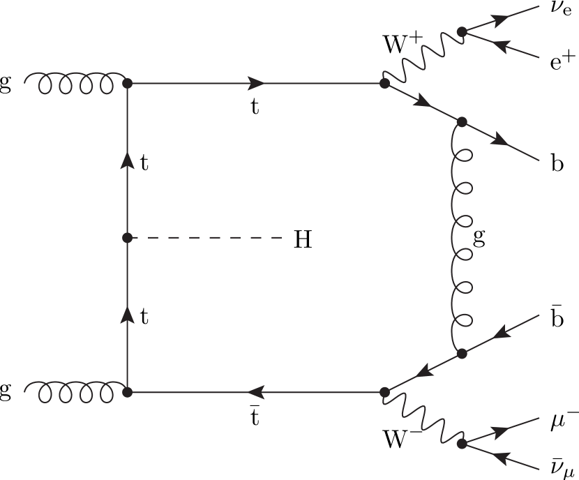
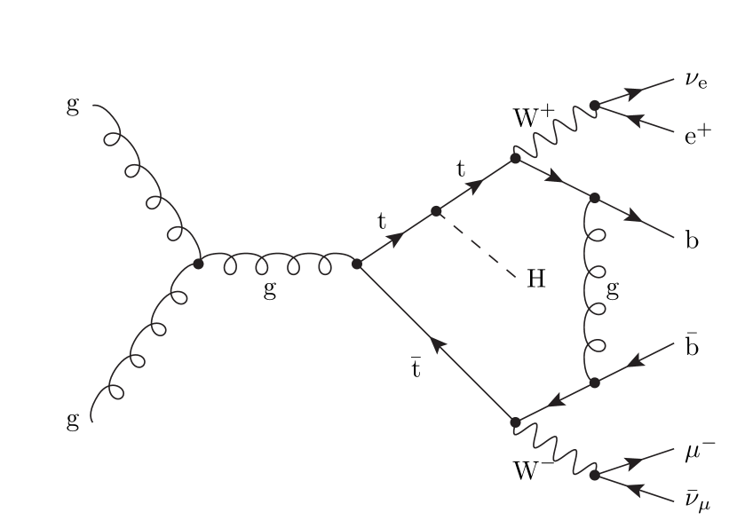
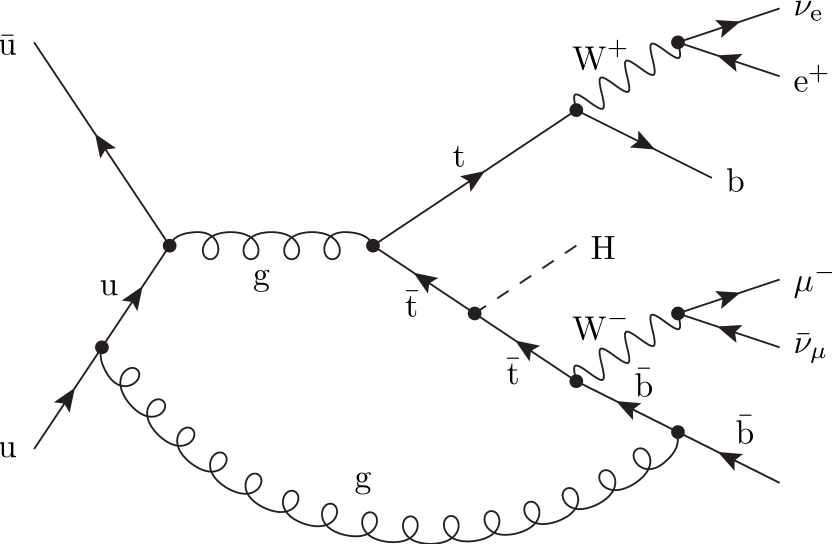
The partonic subprocesses for the virtual QCD corrections can be identified with those at LO. We compute the virtual corrections in the ’t Hooft–Feynman gauge, where the gg process involves 9074 loop diagrams and the processes 2404 loop diagrams each. The most complicated one-loop diagrams are heptagons (Sample diagrams are displayed in Figure 2).
The resonant top quarks, Z bosons and W bosons are treated in the complex-mass scheme Denner:1999gp ; Denner:2005fg ; Denner:2006ic , where the masses of unstable particles are consistently treated as complex quantities leading in particular to a complex weak mixing angle,
| (3) |
For the renormalization we use the on-shell renormalization scheme as described in Ref. Denner:2005fg for the complex-mass scheme.
For the computation of the matrix elements for the virtual corrections we employ Recola Actis:2012qn in dimensional regularisation, which integrates the Collier Denner:2014gla ; Collier library for the numerical evaluation of one-loop scalar 'tHooft:1978xw ; Beenakker:1988jr ; Dittmaier:2003bc ; Denner:2010tr and tensor integrals Passarino:1978jh ; Denner:2002ii ; Denner:2005nn . We compared our results for the virtual NLO contribution to the squared amplitude, , for many phase-space points with MadGraph5_aMC@NLO Alwall:2014hca (see Section 4 for details).
3 Numerical Results
3.1 Input parameters, jet definition, cuts and scale choice
We present results for integrated cross sections and differential distributions for the LHC operating at . For the computation of the hadronic cross section we employ LHAPDF 6.05 with CT10NLO parton distributions at LO and NLO QCD. We use the value of the strong coupling constant as provided by LHAPDF based on a one-loop (two-loop) accuracy at LO (NLO) with active flavours. In the renormalization of the top-quark loop in the gluon self-energy is subtracted at zero momentum. The running of in this scheme is generated by contributions from light-quark and gluon loops only. For the fixed renormalization and factorization scale , defined below in (13), we find
| (4) |
We neglect contributions from the suppressed bottom-quark parton density.
The electromagnetic coupling is derived from the Fermi constant in the scheme Denner:2000bj ,
| (5) |
We compute the width of the top quark for unstable W bosons and massless bottom quarks according to Ref. Jezabek:1988iv . At NLO QCD it reads
| (6) |
with , , and
| (7) | ||||
| (8) |
For the top-quark width at LO we neglect the correction term .
As input, we employ the following numerical values for the masses and widths:
| (9) | ||||||||
which includes the measured value of the Higgs-boson mass with zero width since we assume it to be stable. We neglect the masses and widths of all other quarks and leptons.
We convert the measured on-shell values (OS) for the masses and widths of the W and Z boson into pole values for the gauge bosons () according to Ref. Bardin:1988xt ,
| (10) |
that enter the calculation.
We use the anti- algorithm Cacciari:2008gp for the jet reconstruction with a jet-resolution parameter . The distance between two jets and in the rapidity–azimuthal plane is defined as
| (11) |
with the azimuthal angle and the rapidity of jet , where is the energy and the component of momentum along the beam axis. Only final-state quarks and gluons with rapidity are clustered into infrared-safe jets.
After recombination we impose standard selection cuts on transverse momenta and rapidities of charged leptons and b jets, missing transverse momentum and distance between b jets according to (11). We require two b jets and two charged leptons in the final state, with bottom quarks in jets leading to b jets, and
| b jets: | (12) | |||||||
| charged lepton: | ||||||||
| missing transverse momentum: | ||||||||
| b-jet–b-jet distance: | ||||||||
We have identified the renormalization scale with the factorization scale and have considered a fixed reference scale set to half the partonic threshold energy for production according to Ref. Beenakker:2002nc :
| (13) |
Alternatively, we use a dynamical scale following Ref. Frederix:2011zi
| (14) |
which corresponds to the geometric mean of the top-quark, antitop-quark and Higgs-boson transverse masses. For the comparison of the scale choices we compute the logarithmic scale average of the dynamical scale, defined as
| (15) |
The scale uncertainty of the LO and NLO cross section is determined by variation of the renormalization and factorization scales and around the central value and for the fixed and dynamical scale choice, respectively.. While varying the renormalization scale in PDFs and matrix elements, the top-quark width remains fixed as computed at the top-quark mass according to (6). For the investigation of the scale dependence of the integrated cross section in Figure 4 we vary the scale up and down by a factor of eight for the LO and NLO integrated cross section for the three cases: 1) , 2) , , 3) , . While we show all three cases for the dynamical scale, we show only the first case for the fixed scale choice in Figure 4. For all other results, i.e. those in Table 1 and Figures 5–7, the scale uncertainties are determined from factor-two variations as follows. We compute integrated and differential cross sections at seven scale pairs, , . The central value corresponds to , and the error band is constructed from the envelope of these seven calculations.
3.2 Integrated cross section and scale dependence
| ch. | [fb] | [fb] | ||
|---|---|---|---|---|
| gg | 1.273(2) | |||
| 0.733(2) | ||||
| g ( ) | ||||
| pp | 1.172(1) | |||
| gg | 1.282(2) | |||
| 0.737(2) | ||||
| g ( ) | ||||
| pp | 1.176(1) |
In Table 1 we present the integrated cross sections with fixed (13) and dynamical scale (14) at the LHC at corresponding to the input parameters (4), (5) and (9) and the cuts as defined in (12). The results include only contributions of for LO amplitudes and the corresponding QCD corrections. We neglect possible contributions to processes of for LO amplitudes, which we determined to be about 2 per mille of the integrated cross section at LO for the setup described above. We also do not include partonic channels with incoming bottom quarks. At LO and using the dynamical scale (14), these contribute , i.e. , to the integrated cross section. Moreover, we calculated the integrated cross section at LO with finite bottom-quark masses, leading to a reduction of the cross section for our set of cuts by 0.03%.
The use of the dynamical scale instead of the fixed scale increases the LO and NLO cross sections by only about 1 %, and the factor is 1.172 for the dynamical scale and 1.176 for the fixed scale. The similar quality of both scale choices is also supported by the logarithmic scale average of the dynamical scale as defined in (15). With it corresponds to a slight effective decrease of the fixed scale by only about 6 %.
Since integrated cross sections and NLO effects are very similar, the following considerations hold true for both, the dynamical and fixed scale: The major contributions to the cross section originate from the gluon-fusion process, with about 70 % at LO while increasing at NLO to 76 %. The contribution of the quark–antiquark annihilation drops from about 30 % at LO to 19 %. At NLO the gluon–(anti)quark induced real-radiation subprocesses contribute about 5 % to the integrated cross section. The inclusion of NLO QCD corrections reduces the scale dependence from 31 % to 5 %.
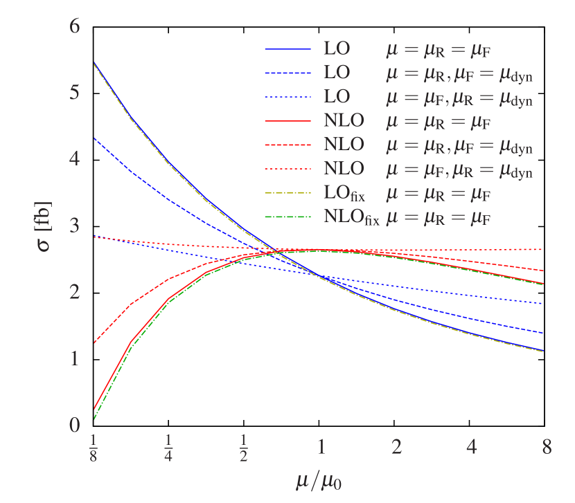
We display the dependence of the integrated LO (blue) and NLO (red) cross sections on the values of the fixed and dynamical scale in Figure 4. Solid lines for the dynamical scale and dash-dotted lines for the fixed scale show the scale dependence for a simultaneous variation of the renormalization and factorization scales and dashed lines the individual variation, where one of the scales is kept fix at the central value, for the dynamical scale only. While the largest scale variation is obtained when both scales are changed simultaneously, the smallest effect results if only the factorization scale is varied. The cross sections for the fixed and dynamical scale choices are uniformly shifted relative to each other by about 1 % as for the central scale both for LO and NLO except for , where the fixed scale leads to a faster decrease of the cross section with as the dynamical scale. For the fixed and dynamical scale the maximum of the NLO cross section is near , justifying the use of both scale choices to be stable against scale variations. The factor equals one at the slightly lower scale of about
3.3 Limit of on-shell top quarks
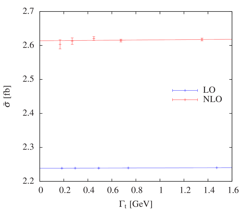
To determine the effects of non-resonant and off-shell top-quark contributions on the integrated cross section we perform a numerical extrapolation to the zero-top-width limit, . To this end we plot
| (16) |
in the range , where is the top-quark width at LO and NLO, resp., and extrapolate linearly to , using a linear regression based on the computed LO and NLO integrated cross sections, as shown in Figure 4. The factor restores the physical top-decay branching fraction. Finite-top-width effects can be extracted by comparing the results for to . At the LHC at for fixed scale finite-top-width effects shift the LO and NLO cross section by and , respectively, which are within the expected order of . The strong suppression of finite-top-width effects is related to the requirement of a final state with two hard b jets. Finite-width effects are much more sizable in calculations where phase-space regions allowing for associated single-top plus W-boson production are included Cascioli:2013wga . Such calculations require massive bottom quarks to regularize collinear singularities.
3.4 Differential distributions
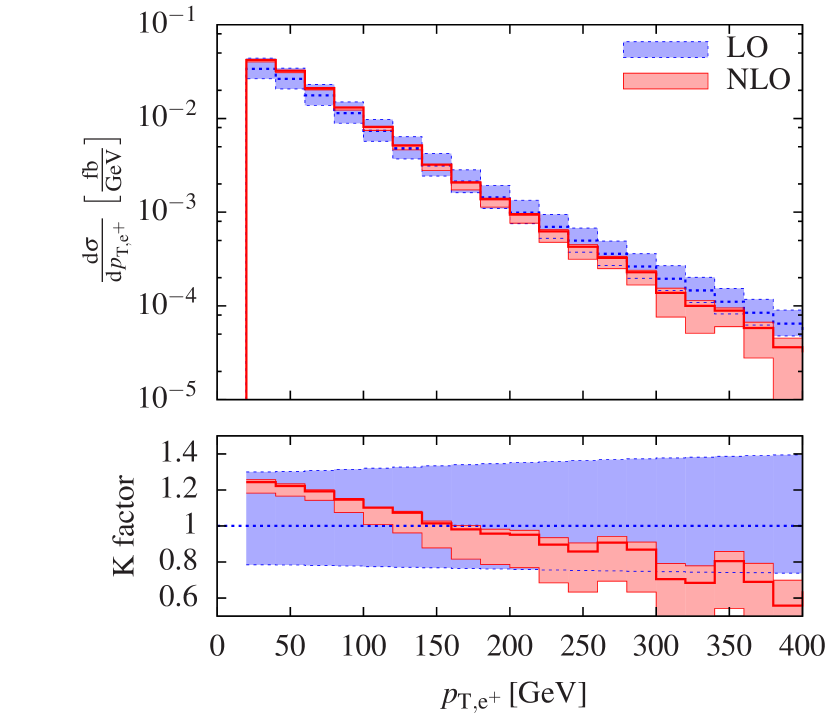
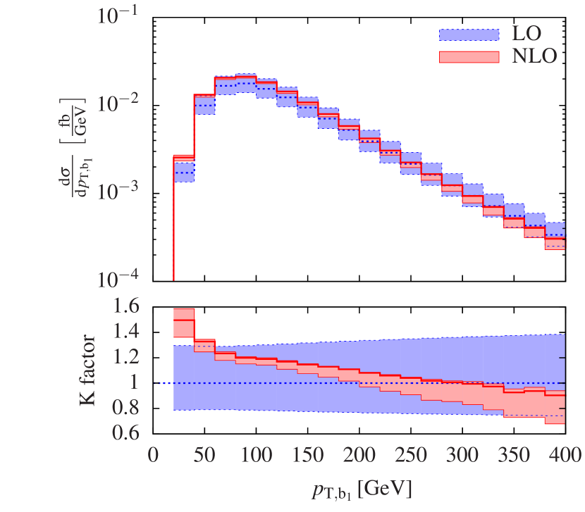
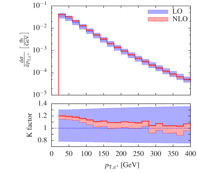
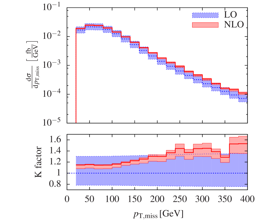
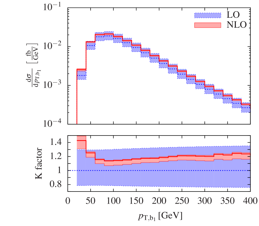
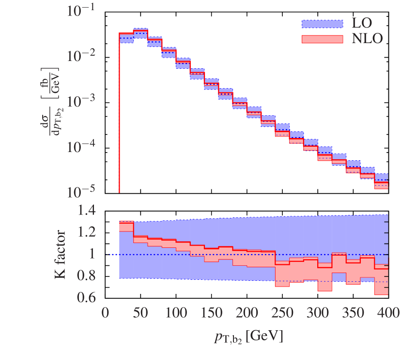
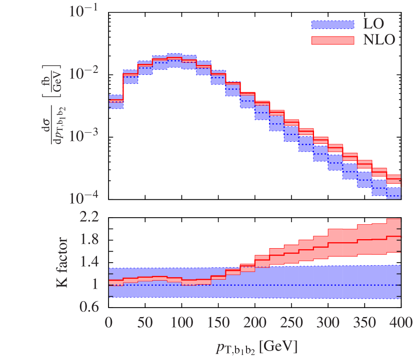
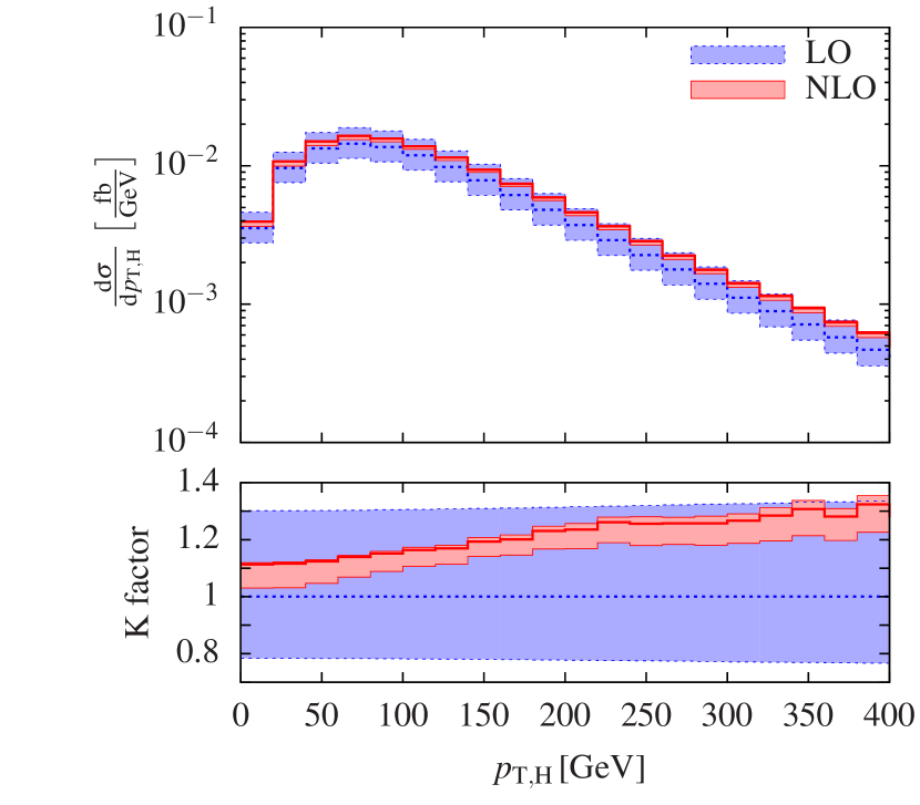
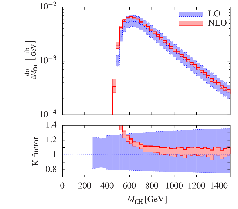
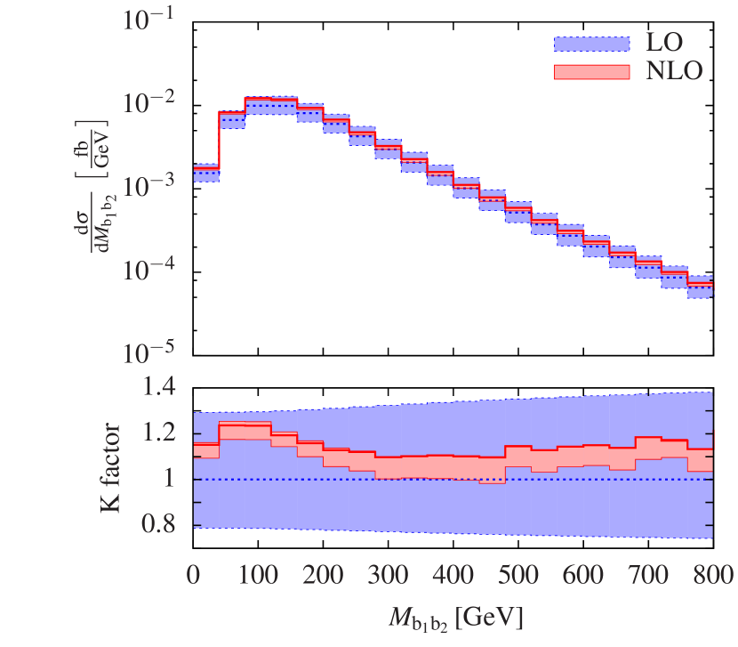
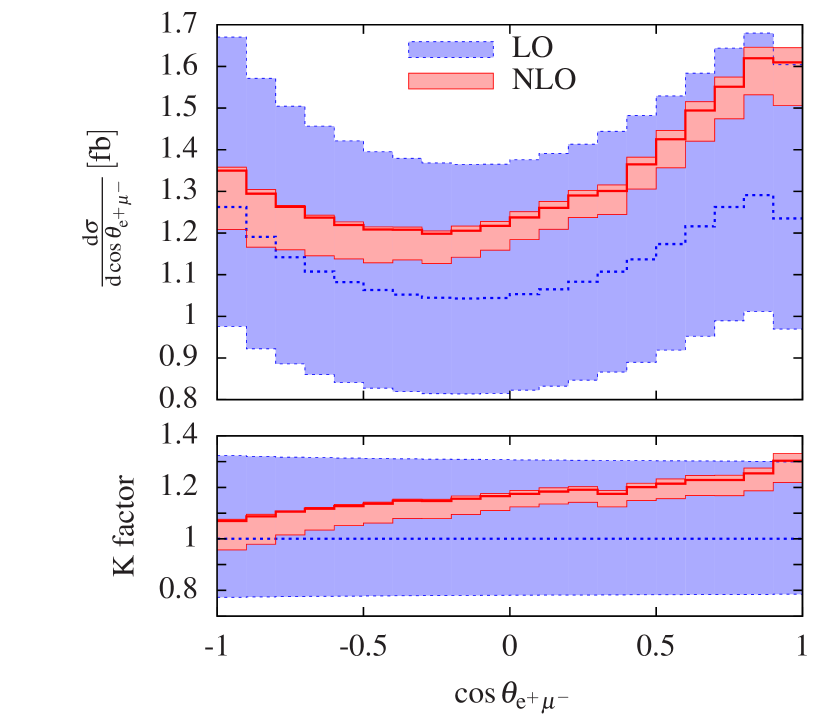
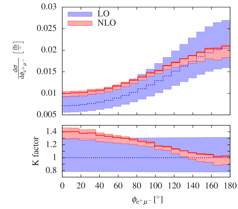
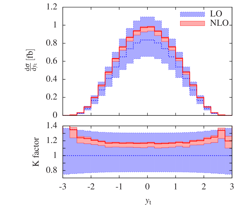
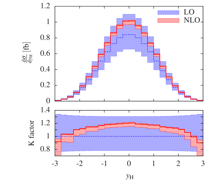
In this section we present various differential distributions with two plots for each observable: The upper plot showing the LO (blue, dashed) and NLO (red, solid) predictions with uncertainty bands from the envelope of scale variations by seven pairs, ,. The lower plot displays the LO (blue) and NLO (red) predictions normalized to the LO results at the central scale, i.e. and . Thus, the central red curve corresponds to the usual NLO correction factor ( factor), defined as . The blue band shows the relative scale uncertainty of the LO differential cross section.
Most of the displayed differential distributions were obtained using the dynamical scale , except for Figure 5 which illustrates the effect of the fixed-scale choice on transverse-momentum distributions.
Where appropriate we compare NLO effects in differential distributions to those of the related process presented in Ref. Denner:2012yc . In general we find similar NLO effects for most of the distributions, but being often more distinct for in Ref. Denner:2012yc .
Figures 5(a) and 5(b) display the transverse-momentum distributions of the positron and the harder b jet, resp., for the fixed scale . The factor of the transverse-momentum of the positron drops by about 50 % within the plotted range. In the high- tail the NLO predictions move outside the LO band with a scale variation of almost the same size as the LO one. The factor of the transverse-momentum of the harder b jet exhibits the same tendency, but not as drastic as for the positron. It moves outside the LO band for with larger scale variation as at the average of around 90 GeV.
In Figure 6 we collect several transverse momentum distributions obtained using the dynamical scale . Figures 6(a) and 6(c) show the transverse-momentum distributions of the positron and the harder b jet, resp., to compare with the fixed-scale distributions in Figures 5(a) and 5(b) described above: They show clearly that the dynamical-scale choice improves the perturbative stability. The factor changes only slightly (within 20 %) over the displayed range, and the NLO band lies within the LO band. The residual scale variation is at the level of at NLO.
In Figure 6(b) the distribution of missing transverse momentum, defined as , is shown. The factor rises for up to about 1.5.
Figures 6(c) and 6(d) display the distribution of the transverse momentum of the harder and softer b jet, resp. While the factor for the harder b jet exhibits a minimum at the maximum of the distribution and slightly rises towards its tail, the factor of the softer b jet decreases by about 30 % in the plotted range.
The distribution of the transverse momentum of the b-jet pair in Fig. 14 of Ref. Denner:2012yc exhibits a strong suppression of the cross section at LO above . This is due to the fact that in narrow-top-width approximation the b quarks are boosted via their parent top and antitop quark, which have opposite transverse momenta resulting in a suppression of a system with high at LO. The lesser stringent kinematical constraints at NLO result in an enhancement of the cross section and thus a large factor for high . For the production at hand a Higgs boson acquiring transverse momentum softens the kinematical constraint already at LO leading to smaller NLO corrections for high , which can be seen in Figure 6(e). Furthermore, the factor of the distribution resembles the factor of the missing transverse momentum due to a kinematically similar configuration, but with a stronger increase to a value of 1.8 at .
Figure 6(f) displays the transverse-momentum distribution of the Higgs boson. The average of the Higgs boson is around 70 GeV. The cross section decreases more moderately with in the plotted range than for other transverse momentum distributions presented in Figure 6.
In Figure 7 we present further differential distributions for other types of observables: the invariant mass of the and system in Figure 7(a) and Figure 7(b), resp., the cosine of the angle between the two charged leptons in Figure 7(c), the azimuthal angle in the transverse plane between them in Figure 7(d), and the rapidity of the top quark and the Higgs boson in Figure 7(e) and Figure 7(f), resp. Large NLO corrections appear in the distribution below the threshold. These arise dominantly from real gluon bremsstrahlung contributions, where the emitted gluon is not recombined with the bottom quarks and thus does not contribute to . The distribution of the azimuthal angle in the transverse plane between the two charged leptons exhibits sizeable NLO effects for small angles similarly as the distribution in the cosine of the angle between the two charged leptons. The factor varies by for these distributions. The rapidity distribution of the Higgs boson features about the typical NLO effects in the central detector region, which disappear going into forward or backward direction. The factor of the top-quark rapidity distribution on the other hand is almost flat at the level of the NLO effects of the integrated cross section.
4 Checks
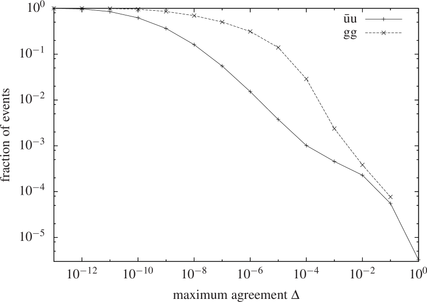
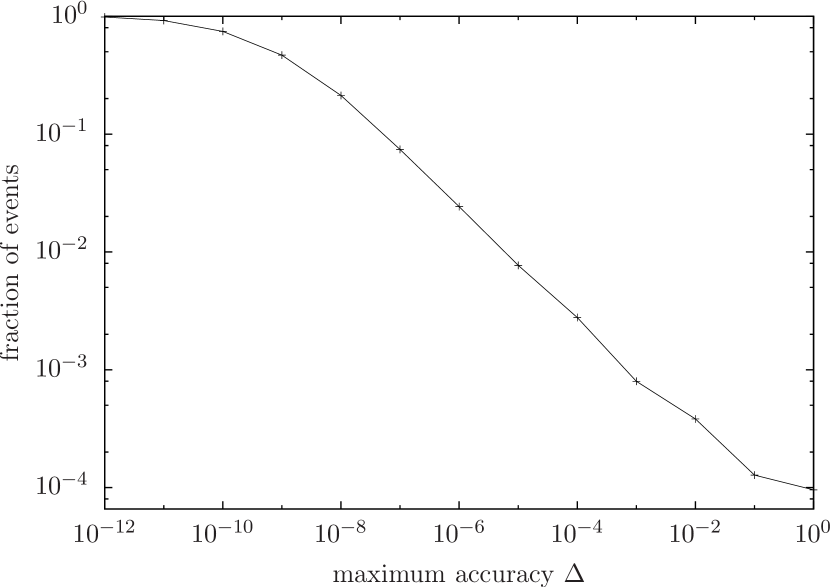
We have performed several comparisons and consistency checks of our calculation. We have reproduced the LO hadronic cross sections with MadGraph5_aMC@NLO Alwall:2014hca using the fixed scale choice. We also compared the virtual NLO contribution to the squared amplitude, , for the gg and subprocesses computed by Recola Actis:2012qn for many phase-space points with MadGraph5_aMC@NLO. In Figure 8(a) we plot the cumulative fraction of events with a relative difference larger than between obtained by Recola and MadGraph5_aMC@NLO. The median of agreement is about for the gg subprocess and roughly for the subprocess. The agreement is worse than for less than 0.3 % of gg- and less than 0.04 % of -subprocess events. For the gg process we checked the accuracy of virtual matrix elements in satisfying the Ward identity, by replacing the polarization vector of one of the initial-state gluons in the one-loop amplitude by its momentum normalized to its energy: . In Figure 8(b) we plot the cumulative fraction of events with for virtual events obtained by Recola with a median of about .
With the Monte Carlo code we developed for the calculation of the process , which employs Recola for the evaluation of matrix elements, we reproduced the results of Ref. Denner:2012yc for the closely related process for the LHC at using a dynamical scale. Since the Catani–Seymour dipoles Catani:1996vz ; Catani:2002hc are the same for the process without the Higgs boson, this comparison allows us to test the implementation of the subtraction formalism. As we use the same renormalization procedure as in Ref. Denner:2012yc , this is also verified via this comparison. In Ref. Denner:2012yc the one-loop matrix elements and the -operator are computed in double-pole approximation for the two W-boson resonances using physical (i.e. real) W- and Z-boson masses and . Moreover, the limit is adopted, i.e. closed fermion loops involving top quarks coupled to Higgs bosons are neglected. In contrast, the new code computes the full one-loop matrix elements and the -operator without any approximation. The largest difference between both calculations results from the use of the double-pole approximation for the virtual corrections and is of order . We could reproduce the results of Ref. Denner:2012yc for the integrated cross section at NLO within , which is at the level of 0.5 %, thus confirming both calculations basically within the accuracy of the numerical integration.
We compared our predictions for the NLO total hadronic cross section with computations of production without decays of the top quarks at NLO for fixed Beenakker:2002nc and dynamical scale Frederix:2011zi . To this end we performed NLO computations using the references’ parameters and PDF mappings and a minimal set of cuts on the decay products of the top and antitop in our process. Since our calculation includes background processes to production, a minimal set of cuts has to be maintained to ensure infrared safety: to avoid large contributions from possible collinear events with bottom quarks in forward direction (as induced by diagrams shown in Figure 1(g) or Figure 1(h)) we kept a small b-jet transverse-momentum cut () and a small b-jet distance cut () to avoid singular events from gluon splitting () as in Figure 1(i). We multiply appropriate branching ratios to the results of Refs. Beenakker:2002nc ; Frederix:2011zi in the narrow-top-width approximation (NtWA), i.e. , and apply the NLO matching prescription of Section 2.1.2 in Ref. Denner:2012yc to our results. Thus, we find agreement of our NLO predictions with Ref. Beenakker:2002nc and Ref. Frederix:2011zi within 1 %, which is of the expected order of , since our calculation includes off-shell and non-resonant top-quark effects.
5 Conclusions
In this article we have presented the calculation of the next-to-leading-order QCD corrections to off-shell top–antitop production in association with a Higgs boson with leptonic decay of the top quarks at the LHC, including all resonant, non-resonant, and off-shell effects of top quarks as well as all interferences. For the computation of leading- and next-to-leading-order matrix elements we have utilised the recursive matrix-element generator Recola linked to the one-loop integral library Collier. The phase-space integration has been performed with an in-house multi-channel Monte-Carlo code that implements the dipole subtraction formalism.
We provided integrated cross sections and several differential distributions for a 13 TeV LHC using a fixed and a dynamical scale that have both been used in the literature for the computation of NLO QCD corrections of production with a stable Higgs boson and stable top quarks. We find almost the same integrated cross sections and scale dependence for both scale choices at leading order as well as next-to-leading order QCD, with a similar factor of 1.172 and 1.176 for the dynamical and fixed scale choice, resp. However, the use of the dynamical scale instead of the fixed scale improves the perturbative stability in high-energy tails of most distributions, especially those of transverse momenta. Using the dynamical scale, we find factors in the range and residual scale uncertainties are the level or for distributions. For the integrated cross section an extrapolation to the zero-top-width limit has been performed, indicating non-resonant and off-shell top-quark effects below one per cent. While this effect is small, our calculation is also the first one to include NLO correction effects in the top–antitop–Higgs-boson production and the top decay processes.
Besides its phenomenological relevance, this calculation demonstrates the power of the tools Recola and Collier in performing complicated NLO calculations.
Acknowledgements.
This work was supported by the Bundesministerium für Bildung und Forschung (BMBF) under contract no. 05H12WWE.References
- (1) ATLAS Collaboration, G. Aad et al., Observation of a new particle in the search for the Standard Model Higgs boson with the ATLAS detector at the LHC, Phys.Lett. B716 (2012) 1–29, [arXiv:1207.7214].
- (2) CMS Collaboration, S. Chatrchyan et al., Observation of a new boson at a mass of 125 GeV with the CMS experiment at the LHC, Phys.Lett. B716 (2012) 30–61, [arXiv:1207.7235].
- (3) R. Raitio and W. W. Wada, Higgs Boson Production at Large Transverse Momentum in QCD, Phys.Rev. D19 (1979) 941.
- (4) J. N. Ng and P. Zakarauskas, A QCD Parton Calculation of Conjoined Production of Higgs Bosons and Heavy Flavors in Collision, Phys.Rev. D29 (1984) 876.
- (5) Z. Kunszt, Associated Production of Heavy Higgs Boson with Top Quarks, Nucl.Phys. B247 (1984) 339.
- (6) J. Gunion, Associated top anti-top Higgs production as a large source of W H events: Implications for Higgs detection in the final state, Phys.Lett. B261 (1991) 510–517.
- (7) W. J. Marciano and F. E. Paige, Associated production of Higgs bosons with pairs, Phys.Rev.Lett. 66 (1991) 2433–2435.
- (8) W. Beenakker, S. Dittmaier, M. Krämer, B. Plümper, M. Spira, et al., Higgs radiation off top quarks at the Tevatron and the LHC, Phys.Rev.Lett. 87 (2001) 201805, [hep-ph/0107081].
- (9) W. Beenakker, S. Dittmaier, M. Krämer, B. Plümper, M. Spira, et al., NLO QCD corrections to production in hadron collisions, Nucl.Phys. B653 (2003) 151–203, [hep-ph/0211352].
- (10) L. Reina and S. Dawson, Next-to-leading order results for production at the Tevatron, Phys.Rev.Lett. 87 (2001) 201804, [hep-ph/0107101].
- (11) S. Dawson, L. Orr, L. Reina, and D. Wackeroth, Associated top quark Higgs boson production at the LHC, Phys.Rev. D67 (2003) 071503, [hep-ph/0211438].
- (12) S. Dawson, C. Jackson, L. Orr, L. Reina, and D. Wackeroth, Associated Higgs production with top quarks at the large hadron collider: NLO QCD corrections, Phys.Rev. D68 (2003) 034022, [hep-ph/0305087].
- (13) R. Frederix, S. Frixione, V. Hirschi, F. Maltoni, R. Pittau, et al., Scalar and pseudoscalar Higgs production in association with a top-antitop pair, Phys.Lett. B701 (2011) 427–433, [arXiv:1104.5613].
- (14) M. Garzelli, A. Kardos, C. Papadopoulos, and Z. Trócsányi, Standard Model Higgs boson production in association with a top anti-top pair at NLO with parton showering, Europhys.Lett. 96 (2011) 11001, [arXiv:1108.0387].
- (15) H. B. Hartanto, B. Jäger, L. Reina, and D. Wackeroth, Higgs boson production in association with top quarks in the POWHEG BOX, Phys. Rev. D91 (2015) 094003, [arXiv:1501.04498].
- (16) S. Frixione, V. Hirschi, D. Pagani, H. S. Shao, and M. Zaro, Weak corrections to Higgs hadroproduction in association with a top-quark pair, JHEP 1409 (2014) 065, [arXiv:1407.0823].
- (17) Z. Yu, M. Wen-Gan, Z. Ren-You, C. Chong, and G. Lei, QCD NLO and EW NLO corrections to production with top quark decays at hadron collider, Phys.Lett. B738 (2014) 1–5, [arXiv:1407.1110].
- (18) S. Frixione, V. Hirschi, D. Pagani, H. S. Shao, and M. Zaro, Electroweak and QCD corrections to top-pair hadroproduction in association with heavy bosons, arXiv:1504.03446.
- (19) A. Bredenstein, A. Denner, S. Dittmaier, and S. Pozzorini, NLO QCD corrections to production at the LHC: 1. Quark-antiquark annihilation, JHEP 0808 (2008) 108, [arXiv:0807.1248].
- (20) A. Bredenstein, A. Denner, S. Dittmaier, and S. Pozzorini, NLO QCD corrections to at the LHC, Phys.Rev.Lett. 103 (2009) 012002, [arXiv:0905.0110].
- (21) G. Bevilacqua, M. Czakon, C. Papadopoulos, R. Pittau, and M. Worek, Assault on the NLO Wishlist: , JHEP 0909 (2009) 109, [arXiv:0907.4723].
- (22) A. Bredenstein, A. Denner, S. Dittmaier, and S. Pozzorini, NLO QCD Corrections to Top Anti-Top Bottom Anti-Bottom Production at the LHC: 2. full hadronic results, JHEP 1003 (2010) 021, [arXiv:1001.4006].
- (23) G. Bevilacqua, M. Czakon, C. G. Papadopoulos, and M. Worek, Dominant QCD Backgrounds in Higgs Boson Analyses at the LHC: A Study of jets at Next-To-Leading Order, Phys. Rev. Lett. 104 (2010) 162002, [arXiv:1002.4009].
- (24) G. Bevilacqua, M. Czakon, C. G. Papadopoulos, and M. Worek, Hadronic top-quark pair production in association with two jets at Next-to-Leading Order QCD, Phys. Rev. D84 (2011) 114017, [arXiv:1108.2851].
- (25) G. Bevilacqua and M. Worek, On the ratio of and cross sections at the CERN Large Hadron Collider, JHEP 07 (2014) 135, [arXiv:1403.2046].
- (26) A. Kardos and Z. Trócsányi, Hadroproduction of t anti-t pair with a b anti-b pair using PowHel, J.Phys. G41 (2014) 075005, [arXiv:1303.6291].
- (27) F. Cascioli, P. Maierh fer, N. Moretti, S. Pozzorini, and F. Siegert, NLO matching for production with massive b-quarks, Phys. Lett. B734 (2014) 210–214, [arXiv:1309.5912].
- (28) M. V. Garzelli, A. Kardos, and Z. Tr cs nyi, Hadroproduction of final states at LHC: predictions at NLO accuracy matched with Parton Shower, JHEP 03 (2015) 083, [arXiv:1408.0266].
- (29) S. Höche, F. Krauss, P. Maierhöfer, S. Pozzorini, M. Schönherr, and F. Siegert, Next-to-leading order QCD predictions for top-quark pair production with up to two jets merged with a parton shower, Phys. Lett. B748 (2015) 74–78, [arXiv:1402.6293].
- (30) ATLAS Collaboration, Search for the Standard Model Higgs boson produced in association with top quarks in proton-proton collisions at TeV using the ATLAS detector, ATLAS-CONF-2012-135, ATLAS-COM-CONF-2012-162.
- (31) ATLAS Collaboration, Search for the Standard Model Higgs boson produced in association with top quarks and decaying to in pp collisions at 8 TeV with the ATLAS detector at the LHC, ATLAS-CONF-2014-011, ATLAS-COM-CONF-2014-004.
- (32) ATLAS Collaboration, G. Aad et al., Search for produced in association with top quarks and constraints on the Yukawa coupling between the top quark and the Higgs boson using data taken at 7 TeV and 8 TeV with the ATLAS detector, Phys. Lett. B740 (2015) 222–242, [arXiv:1409.3122].
- (33) ATLAS Collaboration, Search for the associated production of the Higgs boson with a top quark pair in multi-lepton final states with the ATLAS detector, ATLAS-CONF-2015-006, ATLAS-COM-CONF-2015-008.
- (34) ATLAS Collaboration, G. Aad et al., Search for the Standard Model Higgs boson produced in association with top quarks and decaying into in pp collisions at = 8 TeV with the ATLAS detector, Eur. Phys. J. C75 (2015) 349, [arXiv:1503.05066].
- (35) CMS Collaboration, Search for Higgs boson production in association with top quark pairs in pp collisions, CMS-PAS-HIG-12-025.
- (36) CMS Collaboration, Search for Higgs Boson Production in Association with a Top-Quark Pair and Decaying to Bottom Quarks or Tau Leptons, CMS-PAS-HIG-13-019.
- (37) CMS Collaboration, Search for ttH production in events where H decays to photons at 8 TeV collisions, Tech. Rep. CMS-PAS-HIG-13-015, CERN, Geneva, 2013.
- (38) CMS Collaboration, S. Chatrchyan et al., Search for the standard model Higgs boson produced in association with a top-quark pair in pp collisions at the LHC, JHEP 1305 (2013) 145, [arXiv:1303.0763].
- (39) CMS Collaboration, V. Khachatryan et al., Search for the associated production of the Higgs boson with a top-quark pair, JHEP 1409 (2014) 087, [arXiv:1408.1682]. Erratum: ibid 10 (2014) 106.
- (40) CMS Collaboration, V. Khachatryan et al., Search for a standard model Higgs boson produced in association with a top-quark pair and decaying to bottom quarks using a matrix element method, Eur.Phys.J. C75 (2015) 251, [arXiv:1502.02485].
- (41) S. Dittmaier and M. Roth, LUSIFER: A LUcid approach to six FERmion production, Nucl.Phys. B642 (2002) 307–343, [hep-ph/0206070].
- (42) S. Catani and M. Seymour, A General algorithm for calculating jet cross-sections in NLO QCD, Nucl.Phys. B485 (1997) 291–419, [hep-ph/9605323]. Erratum-ibid. B510 (1998) 503–504.
- (43) S. Dittmaier, A General approach to photon radiation off fermions, Nucl.Phys. B565 (2000) 69–122, [hep-ph/9904440].
- (44) S. Catani, S. Dittmaier, M. H. Seymour, and Z. Trócsányi, The Dipole formalism for next-to-leading order QCD calculations with massive partons, Nucl.Phys. B627 (2002) 189–265, [hep-ph/0201036].
- (45) L. Phaf and S. Weinzierl, Dipole formalism with heavy fermions, JHEP 0104 (2001) 006, [hep-ph/0102207].
- (46) S. Actis, A. Denner, L. Hofer, A. Scharf, and S. Uccirati, Recursive generation of one-loop amplitudes in the Standard Model, JHEP 1304 (2013) 037, [arXiv:1211.6316].
- (47) A. Denner, S. Dittmaier, S. Kallweit, and S. Pozzorini, NLO QCD corrections to off-shell top-antitop production with leptonic decays at hadron colliders, JHEP 1210 (2012) 110, [arXiv:1207.5018].
- (48) A. Denner, S. Dittmaier, M. Roth, and D. Wackeroth, Predictions for all processes fermions , Nucl.Phys. B560 (1999) 33–65, [hep-ph/9904472].
- (49) A. Denner, S. Dittmaier, M. Roth, and L. Wieders, Electroweak corrections to charged-current fermion processes: Technical details and further results, Nucl.Phys. B724 (2005) 247–294, [hep-ph/0505042]. Erratum-ibid. B854 (2012) 504–507.
- (50) A. Denner and S. Dittmaier, The Complex-mass scheme for perturbative calculations with unstable particles, Nucl.Phys.Proc.Suppl. 160 (2006) 22–26, [hep-ph/0605312].
- (51) A. Denner, S. Dittmaier, and L. Hofer, COLLIER – A fortran-library for one-loop integrals, PoS LL2014 (2014) 071, [arXiv:1407.0087].
- (52) A. Denner, S. Dittmaier, and L. Hofer, “COLLIER: a fortran-based complex one-loop library in extended regularizations.” in preparation.
- (53) G. ’t Hooft and M. J. G. Veltman, Scalar One Loop Integrals, Nucl. Phys. B153 (1979) 365–401.
- (54) W. Beenakker and A. Denner, Infrared divergent scalar box integrals with applications in the electroweak standard model, Nucl. Phys. B338 (1990) 349–370.
- (55) S. Dittmaier, Separation of soft and collinear singularities from one-loop N-point integrals, Nucl. Phys. B675 (2003) 447–466, [hep-ph/0308246].
- (56) A. Denner and S. Dittmaier, Scalar one-loop 4-point integrals, Nucl. Phys. B844 (2011) 199–242, [arXiv:1005.2076].
- (57) G. Passarino and M. J. G. Veltman, One Loop Corrections for Annihilation into in the Weinberg Model, Nucl. Phys. B160 (1979) 151.
- (58) A. Denner and S. Dittmaier, Reduction of one-loop tensor 5-point integrals, Nucl. Phys. B658 (2003) 175–202.
- (59) A. Denner and S. Dittmaier, Reduction schemes for one-loop tensor integrals, Nucl. Phys. B734 (2006) 62–115.
- (60) J. Alwall, R. Frederix, S. Frixione, V. Hirschi, F. Maltoni, et al., The automated computation of tree-level and next-to-leading order differential cross sections, and their matching to parton shower simulations, JHEP 1407 (2014) 079, [arXiv:1405.0301].
- (61) A. Denner, S. Dittmaier, M. Roth, and D. Wackeroth, Electroweak radiative corrections to 4 fermions in double-pole approximation: The RACOONWW approach, Nucl.Phys. B587 (2000) 67–117, [hep-ph/0006307].
- (62) M. Jezabek and J. H. Kühn, QCD corrections to semileptonic decays of heavy quarks, Nucl.Phys. B314 (1989) 1.
- (63) D. Y. Bardin, A. Leike, T. Riemann, and M. Sachwitz, Energy Dependent Width Effects in Annihilation Near the Z Boson Pole, Phys.Lett. B206 (1988) 539–542.
- (64) M. Cacciari, G. P. Salam, and G. Soyez, The Anti-k(t) jet clustering algorithm, JHEP 0804 (2008) 063, [arXiv:0802.1189].
- (65) F. Cascioli, S. Kallweit, P. Maierh fer, and S. Pozzorini, A unified NLO description of top-pair and associated Wt production, Eur. Phys. J. C74 (2014) 2783, [arXiv:1312.0546].