Dynamics of locally coupled agents with next nearest neighbor interaction

Abstract

We consider large but finite systems of identical agents on the line with up to next nearest neighbor asymmetric coupling. Each agent is modelled by a linear second order differential equation, linearly coupled to up to four of its neighbors. The only restriction we impose is that the equations are decentralized. In this generality we give the conditions for stability of these systems. For stable systems, we find the response to a change of course by the leader. This response is at least linear in the size of the flock. Depending on the system parameters, two types of solutions have been found: damped oscillations and reflectionless waves. The latter is a novel result and a feature of systems with at least next nearest neighbor interactions. Analytical predictions are tested in numerical simulations.

1 Introduction

Coupled second order ordinary linear differential equations, coupled oscillators for short, play an important role in almost all areas of science and technology (see the introduction of Lewis2014 for a recent review). The phenomena of coupled systems appear on all length– and time–scales: from synchronization of power generators in power-grid networks Backhaus2013 ; Motter2013 , through the traffic control of vehicular platoons Bamieh2002 ; Cruz2007 ; Defoort2008 ; Lin2012 ; Barooah2013 ; Herman2015 , collective decision-making in biological systems Reynolds1987 ; Strogatz1993 ; Couzin2005 ; Attanasi2014 ; Pearce2014 (e.g., transfer of long–range information in flocks of birds), to the atomic scale lattice vibrations (so-called phonons), just to name few of them. The nature of communication within such a systems crucially influences the behavior of it. In the presence of centralized information, e.g., the knowledge of the desired velocity by members of a flock, the performance of many of these systems is good Bamieh2002 ; Lin2012 ; Barooah2013 in the sense that the trajectories of the agents quickly converge to coherent (or synchronized) motion. On the other hand, in decentralized systems convergence to coherent motion is much less obvious, since no overall goal is observed by all agents. In this case, the only available observations (i.e., of position and/or velocity) are relative to the agent. The complication of the problem is even greater if information is exchanged only locally - by agents in a neighborhood that is small in comparison to the system size.

As an aside, we point out that there exist another class of somewhat similar problems, also with a wide range of applications, namely the dynamics of consensus, see Ren ; Hegselmann . The difference is that in our case the agents are Newtonian (are subject to force $m\ddot{x}$, i.e., mass $\times$ accelerations), whereas in consensus type equation, that is not the case. Therefore consensus equations tend to be coupled first order ordinary differential equations with a very different behavior. In particular, we do not expect to see wave-like behavior in consensus equations, whereas they in our equations those play a prominent role. In what follows we will restrict ourselves to coupled second order differential equations.

It is of significant importance to develop a theory that deals with systems where agents may interact with few nearby agents. In the case of physical systems with symmetric interactions and no damping (such as harmonic crystals), this theory exists and can be found in textbooks Ashcroft1976 . It consists of imposing periodic boundary conditions, and then asserting that the solutions of the periodic system behave the same way as in the system with non-trivial boundary conditions, except near the boundary. Although we know of no formal proof in the literature that this is correct, this method of solution has been used for about a century with great success. Neither is it the case that we can rely on previous studies of discretization of a second order partial differential equation. Indeed the finite difference method applied to a wave equation with convection will give rise (for small enough mesh) to nearly symmetric equations Haberman ; VanLoan .

In flocks there is no reason for the interactions to be symmetric or undamped, as is the case in the study of harmonic crystals. The equations studied here are therefore more general. Furthermore in flocks it is desirable to have a two parameter set of equilibria, namely motion with constant velocity and constant distance between any two consecutive agents (coherent motion). Thus it is necessary to study a more general problem, namely convergence to coherent motion in the presence of asymmetry and damping. In this paper we generalize the previously successful approach (periodic boundary conditions). In doing this one needs to be aware though that (i) assumptions or conjectures needed to solve the old problem must be investigated again as they may not be justified anymore, and (ii) new phenomena may arise. For more details see Cantos2014-1 ; Cantos2014-2 ; Herman2015 .

In the case of linear response theory in solid state physics Ashcroft1976 , when a system of symmetrically coupled undamped oscillators is perturbed, the signal will typically travel through the entire system at constant velocity without damping. In our case, the system is generally either stable or unstable. In the former case the perturbation will die out over time, and in the latter, the perturbation will blow up exponentially in time. However, even in the stable case perturbations may get very large before dying out. The largest amplitude of a perturbed system that is stable, may in fact still grow exponentially in the size of the system. This phenomenon is called flock instability. Just like “normal” instability, flock-instability is an undesirable property, since it makes large flocks unviable. Flock-instability in arrays of coupled oscillators was illustrated in positionpaper , and bears similarity to certain phenomena discovered earlier in fluid mechanics Trefethen1993 ; Trefethen1997 . Thus the first task is to find criteria to identify those systems that are both stable and flock stable.

We thus need to replace the traditional approach using periodic boundary conditions by another that we now outline. For those systems that are stable and flock stable (and only for those), we conjecture that for times of length ${\cal O}(N)$ (where $N$ is the size of the flock) the solutions of the periodic system behave the same way as in the system with non-trivial boundary, except near the boundary where additional effects must be taken into consideration. It turns out that with those constraints the system with periodic boundary condition behaves like a wave-equation. Since the travel time of a wave between the leader (agent $0$) and the last agent (numbered $N$) is proportional to $N$, we can study the dynamics of the perturbed system for times needed up to a finite number of reflections. Due to the asymmetry, wave-packages traveling in the positive $\mathbb{R}$ direction may have a different signal-velocity than waves traveling in the opposite direction. It turns out we can use this effect to achieve either substantial attenuation or magnification of the traveling wave at the boundary near agent $N$.

In the present work we extend this analysis from nearest neighbor systems done in Cantos2014-1 ; Cantos2014-2 to next nearest neighbor (NNN) systems, and in doing that we uncover another new phenomenon. We will see that for stable and flock stable systems there are still two signal velocities, but that in contrast with nearest neighbor systems it is possible that they have the same sign. This means that perturbations can travel (as waves) in only one direction. As a consequence, they cannot be reflected. This type of transient has the counter-intuitive characteristic that they travel through the system in finite time, after which the system finds itself in (almost) perfect equilibrium.

The paper is organized as follows. In Section 2 we define the model of interacting agents. The main line of reasoning of the method is given in Section 3. The stability conditions are given in Section 4. The description of the stable solutions is presented in Section 5. This includes the description of the reflectionless waves on the line, which to the best of our knowledge is a new result. We include extensive numerical analysis in Section 6 to back up our theory.

2 The Equations of Motion of the NNN System

We consider a model of an one–dimensional array of linear damped coupled (up to next nearest neighbor) harmonic oscillators on the line. The oscillators or agents are numbered from 0 to $N$ from right to left. We impose that the system is decentralized, that is: the agents perceive only information about other agents that is relative to themselves, in this case relative position and relative velocity. See Figure 1 for a sketch of information flow.

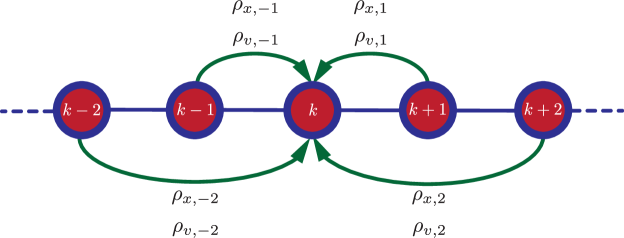
Figure 1: Sketch of information flow. Available information about position $\rho_{x,j}$ and velocity $\rho_{v,j}$ weight of nearest $j=k\pm 1$ and next nearest $j=k\pm 2$ agents for $k$’th agent.

The equations of motion of such a system can be written as:

$$\ddot{x}_{k}=\sum_{j=-2}^{2}\left[g_{x}\rho_{x,j}\left(x_{k+j}-x_{k}+j\,\Delta\right)+g_{v}\rho_{v,j}\left(\dot{x}_{k+j}-\dot{x}_{k}\right)\right]\,,$$ (1)

where $\Delta$ is the desired inter–agent distance and $\rho_{x,j}$ ($\rho_{v,j}$) are position (velocity) parameters. The latter are normalized so that $\rho_{x,0}=\rho_{v,0}=1$. The normalization factors, $g_{x}$ and $g_{v}$, are often called the ‘gains’ in the engineering literature.

The initial conditions we will impose from here on, are as follows. At time $t\leq 0$ the agents are in equilibrium, $x_{k}=-k\,\Delta$. Then, for $t>0$, the leader $x_{0}$ starts moving forward at velocity $v_{0}$:

$$\forall t\geq 0\quad x_{0}(t)=v_{0}t\,.$$

The leader is not influenced by other agents, although other agents (e.g., $k=1$ and $k=2$) are influenced by it. This choice of the leader at the head of the flock is motivated by applications to traffic situations (see Cantos2014-1 ; Cantos2014-2 ). It is possible to analyze the dynamics with leaders in different positions or having more than one leader. We will not pursue this here.

It is convenient to eliminate the constant $\Delta$ from Equation (1), using the change of coordinates: $z_{k}\equiv x_{k}+k\,\Delta$. In this notation, the equation of motion of the flock in $\mathbb{R}$ becomes:

Definition 2.1

The equations of motion of the NNN system with $N>4$ agents, for $k\in\{1,\cdots N\}$, are:

$$\ddot{z}_{k}=\sum_{j=-2}^{2}\left(g_{x}\rho_{x,j}z_{k+j}+g_{v}\rho_{v,j}\dot{z}_{k+j}\right)\,.$$ (2)

This system is subject to the constraints

$$\rho_{x,0}=\rho_{v,0}=1\,,\quad\sum_{j=-2}^{2}\rho_{x,j}=\sum_{j=-2}^{2}\rho_{v,j}=0\,,$$ (3)

and to the initial conditions:

$$z_{k}(0)=0\,,\;\dot{z}_{k}(0)=0\,,\mathrm{and}\,\;z_{0}(t)=v_{0}t\,.$$

From now on we denote this system by ${\cal S}_{N}$. The collection of the systems $\left\{{\cal S}_{N}\right\}_{N>4}$ will be denoted by ${\cal S}$.

Now we use vector notation and write $z\equiv(z_{1},\;z_{2},\;z_{3},\;\dots\;z_{N}\,)^{T}$ together with $\dot{z}\equiv(\dot{z}_{1},\;\dot{z}_{2},\;\dot{z}_{3},\;\dots\;\dot{z}_{N}\,)^{T}$. Equation (2) may be rewritten as a first order system in $2N$ dimensions:

$$\frac{\mathrm{d}}{\mathrm{d}t}\pmatrix{z\cr\dot{z}}=\pmatrix{0&I\cr L_{x}&L_{v}}\pmatrix{z\cr\dot{z}}+F(t)\equiv M_{N}\pmatrix{z\cr\dot{z}}+F(t)\,,$$ (4)

where $L_{x}\,,L_{v}\in\mathbb{R}^{N\times N}$ are matrices - the Laplacians - with standard definition

$$\left(L_{x}z\right)_{k}=\sum_{j=-2}^{2}\,g_{x}\rho_{x,j}z_{k+j}\,,\quad\left(L_{v}\dot{z}\right)_{k}=\sum_{j=-2}^{2}\,g_{v}\rho_{v,j}\dot{z}_{k+j}\,,$$ (5)

where $F(t)$ is the “external force” that describes the influence of the leader with trajectory $z_{0}(t)=v_{0}t$ on the acceleration of its immediate neighbors. It is easy to check that all components are zero except the $N+1$-st and $N+2$-nd components. The exact form of that external force depends of the boundary conditions we choose to impose on the system, as we briefly discuss now.

Note that the equations for $z_{1}$, $z_{N-1}$, and $z_{N}$ are subject to non-trivial boundary conditions (BC), because there are no agents with numbers $-1$, $N+1$, and $N+2$. So the equations of motion for agents $1$, $N-1$, and $N$, will have to be modified. Here we will use two sets of BC: fixed interaction and fixed mass. In the case of fixed interaction BC the central coefficients, $\rho_{x,0}$ and $\rho_{v,0}$, of the boundary agents are not equal $1$, instead it is the sum of existing interactions. On the other hand, in fixed mass BC we change the interactions and keep the central $\rho$’s equal to $1$. The details are given in the Appendix A.

Coherent motion is defined as:

$$y_{k}(t)=a_{0}t+b_{0}-k\,\Delta\,,$$ (6)

where $a_{0}$ and $b_{0}$ are arbitrary real constants. It is easily checked that coherent motion is a solution to the differential equations given above. Our aims are:

1. To find out for which values of the parameters trajectories the system is stable: namely, for all $k$, $\lim_{t\rightarrow\infty}|x_{k}(t)-y_{k}(t)|=0$ where $y_{k}$ is given in Equation (6).

2. To find out how fast the stable systems converge to its coherent motion.

3. To determine what is the size of the transient $\max_{t>0}|x_{N}(t)-y_{N}(t)|$ in stable systems.

In the last item we consider only the last (or $N$-th) agent to simplify the exposition. As an example in Figure 2 we present a sketch of the dynamics expected in the stable system of locally coupled oscillators on the line. In the figures we plot the positions relative to the leader, i.e., $x_{k}(t)-v_{0}t$.

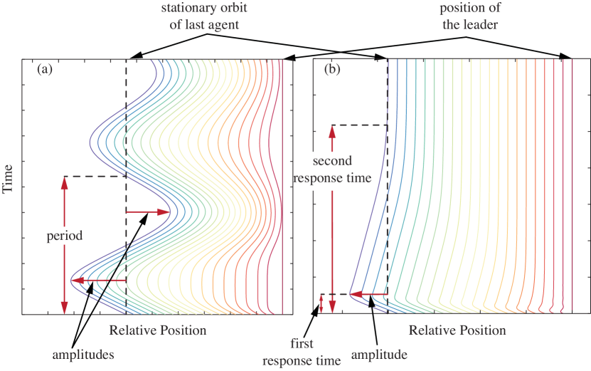
Figure 2: Dynamics of locally coupled arrays. Sketch of time-dependent dynamics of locally coupled oscillators on the line (system ${\cal S}_{N}$) of (a) Type I and (b) Type II (see Section 5 for detailed analysis of these solutions). $x$-axis depicts relative position with respect to the leader.

3 Method

The analysis of the system of Definition 2.1 is very difficult because the Laplacians given in Equation (5) are not simultaneously diagonalizable. In order to overcome that we define a system where the communication structure is not a line graph but a circular graph ( see Figure 3). We use it (in Section 4) to deduce necessary conditions for stability and flock stability on the line, and (in Section 5) to derive expressions for the signal velocities.

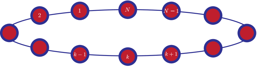
Figure 3: A circular graph. The numbers indicate the labels of the agents.

Definition 3.1

The equations of motion of the system with periodic boundary conditions (PBC) are:

$$\ddot{z}_{k}=\sum_{j=-2}^{2}\left(g_{x}\rho_{x,j}z_{k+j}+g_{v}\rho_{v,j}\dot{z}_{k+j}\right)\,.$$

This system is subject to the constraints

$$\rho_{x,0}=\rho_{v,0}=1\,,\quad\sum_{j=-2}^{2}\rho_{x,j}=\sum_{j=-2}^{2}\rho_{v,j}=0\,.$$

Finally, instead of boundary conditions for $z_{1}$, $z_{N-1}$, and $z_{N}$, we set:

$$\forall j\quad z_{N+j}=z_{j}\,.$$

From now on we denote this system by ${\cal S}^{*}_{N}$. The collection of the systems $\left\{{\cal S}^{*}_{N}\right\}_{N>4}$ will be denoted by ${\cal S}^{*}$.

The Laplacians $L^{*}$ [with the same definition as in Equation (5)] now become circulant matrices and are therefore diagonalizable by the discrete Fourier transform Kra . Let $w_{m}$ be the $m$-th eigenvector of $L^{*}$’s, that is the vector whose $j$-th component satisfies:

$$(w_{m})_{j}=e^{\imath\frac{2\pi m}{N}j}\equiv e^{\imath\phi j}\,,$$

with $\phi=2\pi m/N$. We denote the $m$-th eigenvalues of $L^{*}_{x}$ by $\lambda_{x,m}$ and those of $L^{*}_{v}$ by $\lambda_{v,m}$. With a slight abuse of notation we also consider these eigenvalues to be functions $\lambda_{x}(\phi)$ and $\lambda_{v}(\phi)$ of $\phi$ defined above. By using the $m$-th eigenvector above to calculate $L^{*}_{x}w_{m}$ and $L^{*}_{v}w_{m}$ it is easy to show that:

Lemma 3.1

The $\lambda$’s are given by

$$\lambda_{x}(\phi) = g_{x}\sum_{j=-2}^{2}\rho_{x,j}\,e^{\imath\phi j}=g_{x}\sum_{j=0}^{2}\left[\alpha_{x,j}\,\cos(j\phi)+\imath\beta_{x,j}\,\sin(j\phi)\right]\,,$$

$$\lambda_{v}(\phi) = g_{v}\sum_{j=-2}^{2}\rho_{v,j}\,e^{\imath\phi j}=g_{v}\sum_{j=0}^{2}\left[\alpha_{v,j}\,\cos(j\phi)+\imath\beta_{v,j}\,\sin(j\phi)\right]\,.$$

Here we have used the following convenient notation.

Definition 3.2

Let $\alpha_{x,0}=\alpha_{v,0}=1$ and $\beta_{x,0}=\beta_{v,0}=0$. For $j>0$ we define:

$$\alpha_{x,j}=\rho_{x,j}+\rho_{x,-j}\,,\quad\beta_{x,j}=\rho_{x,j}-\rho_{x,-j}\,,$$

$$\alpha_{v,j}=\rho_{v,j}+\rho_{v,-j}\,,\quad\beta_{v,j}=\rho_{v,j}-\rho_{v,-j}\,.$$

Note that the sum of the $\alpha$’s equals $0$ by Equation (3).

Let us now focus on the eigenvectors and eigenvalues of $M^{*}_{N}$ associated with $w_{m}$. Denoting the eigenvalues by $\nu_{m,\pm}$, we get:

$$\pmatrix{0&I\cr L^{*}_{x}&L^{*}_{v}}\pmatrix{w_{m}\cr\nu_{m,\pm}\,w_{m}}=\nu_{m,\pm}\pmatrix{w_{m}\cr\nu_{m,\pm}\,w_{m}}\,.$$ (7)

Thus the evolution of an arbitrary initial condition is given by:

$$\pmatrix{z(t)\cr\dot{z}(t)}=\sum_{m}\,a_{m}e^{\nu_{m,-}t}\,\pmatrix{w_{m}\cr\nu_{m,-}\,w_{m}}+\sum_{m}\,b_{m}e^{\nu_{m,+}t}\,\pmatrix{w_{m}\cr\nu_{m,+}\,w_{m}}\,,$$ (8)

where the $a_{m}$ and $b_{m}$ are determined by the initial condition at $t=0$.

Next, let us evaluate the second row of Equation (7) using that $w_{m}$ are eigenvectors of $L^{*}$:

Lemma 3.2

The eigenvalues of ${\cal S}^{*}_{N}$ are the roots of the characteristic equation

$$\nu^{2}-\lambda_{v}(\phi)\nu-\lambda_{x}(\phi)=0\,,$$ (9)

where $\phi=2\pi m/N$. The eigenvalues of ${\cal S}^{*}$ are a dense subset of the closed curves $\nu_{+}:S^{1}\rightarrow\mathbb{C}$ and $\nu_{-}:S^{1}\rightarrow\mathbb{C}$ defined by Equation (9).

Our treatment follows that of Cantos2014-2 where it is conjectured that (for nearest neighbor systems) a circular system and a system on the line evolve in a similar manner. The result is that we can analyze the circular system and apply the conclusions to the systems on the line. We briefly outline how the evolution of the two systems can be compared.

First we need to remind the reader of the two notions of stability that play a crucial role in our analysis.

Definition 3.3

For given $N$, the system ${\cal S}_{N}$ (${\cal S}^{*}_{N}$) is asymptotically stable if, given any initial condition, the trajectories always converge to a coherent motion and the convergence is exponential in time. For the systems we consider this is equivalent to: $M_{N}$ ($M^{*}_{N}$) has one eigenvalue zero with multiplicity $2$, and all other eigenvalues have real part (strictly) less than $0$. ${\cal S}_{N}$ (${\cal S}^{*}_{N}$) is unstable if at least one eigenvalue has positive real part.

Flock stability was introduced in positionpaper :

Definition 3.4

The collection ${\cal S}$ is called flock stable if the ${\cal S}_{N}$ are asymptotically stable for all $N$ and if $\mathrm{max}_{t\in\mathbb{R}}|z_{N}(t)|$ grows sub–exponentially in $N$.

Note that asymptotic stability is different from flock stability. The former deals with the growth of the response of a single system as $t$ tends to infinity while $N$ is held fixed, while the latter deals with the growth of the response of a sequence of systems as $N$ tends to infinity.

Now we mention the main ideas that allow us to compare the evolution of the two systems. The first idea is the conjecture that if the system on the circle is asymptotically unstable, then the system on the line is either asymptotically unstable or flock unstable. Notice that undamped, symmetric systems are all marginally stable, and this aspect does not enter the traditional discussion in the physics context. This gives us necessary conditions for stability and flock stability of the system on the line.

The second idea involved in this analysis is the principle that, if the system on the line is stable and flock stable, then the evolution away from the boundary of the two systems should be the same. As we shall see this means that for these systems we obtain wave-like behavior with signal velocities determined by the eigenvalues of the system on the circle (see Theorem 5.1). This is similar to what is commonly known in solid state physics as periodic boundary conditions (see Chapter 21 in Ashcroft1976 ), though not exactly the same. The difference is that here we apply principle in more generality than is usual in physics, because we are considering systems that are not symmetric and not Hamiltonian.

We know that the reverse of this conjecture is actually false: stability on the circle does not imply stability on the line. There are systems that are stable if periodic boundary conditions are imposed, but have some eigenvalues with positive real parts when given non-trivial physical boundary conditions. In Figure 4 we show a simulation of such a system on the line. The parameters are given in the Figure. Another example is given in Section 5. It turns out, perhaps fortunately, that such counter examples are extremely rare.

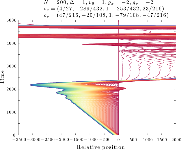
Figure 4: Dynamics of unstable system. Dynamics of example system ${\cal S}_{N}$ as calculated for $N=200$, $\Delta=1$, $v_{0}=1$, $g_{x}=g_{v}=-2$, $\rho_{x}=(4/27,-289/432,1,-253/432,23/216)$, $\rho_{v}=(47/216,-29/108,1,-79/108,-47/216)$ and fixed interaction BC. Each color represents the orbit of one of the $200$ agents.

The third and last idea is that the cumbersome physical boundary conditions of Appendix A may be replaced by a single “free boundary condition” and a single “fixed boundary condition”. This is a great simplification, because the set of possible all physical boundary conditions form a $16$-parameter set, with no obvious naturally “preferred” boundary condition. However because of this last principle, our conclusions will be independent of the physical boundary condition. As before, in the traditional physics context, this problem play little or no role, because presumably the fixed mass BC is the only possible BC.

In extending the principle of periodic boundary conditions and adding some new ideas to it, we need to be aware that new phenomena may appear (see Section 5.2) and indeed its validity is not guaranteed nor is it implied by the validity of the principle in the restricted (symmetric, undamped) case (nor indeed by the validity in the general nearest neighbor case). Thus our conclusions need to be checked numerically (see Section 6).

4 Stability Conditions

We wish to establish conditions that guarantee that the systems ${\cal S}_{N}$ on the line is both asymptotically stable and flock stable. Since a direct verification is too hard or even impossible to perform, we use the conjectures stated in Section 3. According to those, necessary conditions include the stability of the systems ${\cal S}^{*}$, a much simpler problem.

Substituting the expressions for the $\lambda$’s in Lemma 3.1 into Equation (9), we see that the eigenvalues of ${\cal S}^{*}_{N}$ are the roots of the following equation:

$$\nu^{2}-\nu\,g_{v}\sum_{j=-2}^{2}\rho_{v,j}\,e^{\imath\phi j}-g_{x}\sum_{j=-2}^{2}\rho_{x,j}\,e^{\imath\phi j}=0$$ (10)

Note that when $\phi=0$, the characteristic equation becomes $\nu^{2}=0$. This gives two zero eigenvalues. These trivial eigenvalues are associated with the coherent solutions of the system, $z_{k}=0$ [see also Equation (6)].

Lemma 4.1

The following are necessary conditions for ${\cal S}_{N}^{*}$ not to have eigenvalues with positive real part when $N$ is large:

(i)

$\beta_{x,1}+2\beta_{x,2}=0$,

(ii)

$g_{v}\leq 0$,

(iii)

$\alpha_{v,1}\in[-4/3,0]$,

(iv)

$g_{x}\alpha_{x,1}\geq 0$.

Proof: To prove (i) notice that the roots of characteristic Equation (9) are:

$$\nu_{\pm}(\phi)=\frac{1}{2}\left[\lambda_{v}(\phi)\pm\sqrt{\lambda_{v}(\phi)^{2}+4\lambda_{x}(\phi)}\right]\,.$$ (11)

As $\phi=2\pi m/N$ becomes very small, the $\lambda$’s can be approximated by their first order expansion. From Definition 3.2 and Lemma 3.1 we obtain:

$$\lambda_{x}(\phi\to 0)\approx\imath g_{x}\phi\sum_{j=0}^{2}j\beta_{x,j}\,,\quad\lambda_{v}(\phi\to 0)\approx\imath g_{v}\phi\sum_{j=0}^{2}j\beta_{v,j}\,.$$

Substituting these into equation for $\nu$, Equation (11), we see that for small enough $\phi$, the term $\pm\sqrt{4\lambda_{x}(\phi)}$ dominates. Since $\phi$ can be either positive or negative, this has four branches meeting at the origin at angles of $\pi/2$. Two of these branches contain eigenvalues with positive real part (for big enough $N$). Therefore, for $N$ large enough there are $\phi$ such that $\nu_{\pm}(\phi)$ have negative real part unless $\sum_{j=0}^{2}j\beta_{x,j}=0$.

For condition (ii) we note that the mean of the two roots of Equation (11) is equal $\lambda_{v}/2$. It follows that we must require $\Re[\lambda_{v}(\phi)]\leq 0$ for all $\phi\neq 0$. Since the average $\frac{1}{2\pi}\,\int_{-\pi}^{\pi}\Re[\lambda_{v}(\phi)]\mathrm{d}\phi$ is $g_{v}$, there is a $\phi$ so that $\Re[\lambda_{v}(\phi)]\geq g_{v}$. That of course means that $g_{v}$ must be non-positive.

For (iii) note that $\Re[\lambda_{v}(\phi)]\leq 0$. Therefore, $\sum\alpha_{v,j}\cos j\phi\geq 0$. For the NNN system, the constraints on the $\alpha$’s now give

$$1+\alpha_{v,1}\cos(\phi)-(1+\alpha_{v,1})\cos(2\phi)\geq 0\,.$$

Since $\cos(2\phi)=2\cos^{2}\phi-1$, the inequality becomes a quadratic inequality in $\cos(\phi)$:

$$-(2+2\alpha_{v,1})\cos^{2}(\phi)+\alpha_{v,1}\cos\phi+2+\alpha_{v,1}\geq 0\,,$$

which factors as:

$$-\left[(2+2\alpha_{v,1})\cos(\phi)+2+\alpha_{v,1}\right]\left(\cos(\phi)-1\right)\geq 0\,.$$

By working out three cases, $\alpha_{v,1}<-1$, $\alpha_{v,1}=-1$, and $\alpha_{v,1}>-1$, the conclusion of (iii) may be verified.

Beside $\phi=0$, one other case of Equation (9) is easy, namely $\phi=\pi$ with the $\lambda$’s as defined in Lemma 3.1

$$\nu^{2}-\nu g_{v}\sum_{j=0}^{2}(-1)^{j}\alpha_{v,j}-g_{x}\sum_{j=0}^{2}(-1)^{j}\alpha_{x,j}=0\,.$$

The roots have non-positive real part if and only if both coefficients are nonnegative. In particular, this implies that last term in the above equation is $g_{x}\sum_{j=0}^{2}{(-1)^{j}\alpha_{x,j}}\leq 0$. From Definition 3.2 we know that $\sum_{j=0}^{2}{\alpha_{x,j}}=1+\sum_{j=1}^{2}{\alpha_{x,j}}=0$, and as a consequence $g_{x}\alpha_{x,1}\geq 0$, which is condition (iv). Similarly, $g_{v}\alpha_{v,1}\geq 0$ but this already follows from conditions (ii) and (iii). ∎

Since we are only interested in the parameter values for which the collection ${\cal S}^{*}$ is not unstable, we use the above Lemma 4.1 and Definition 3.2 to eliminate a few parameters from our equations. This is done by eliminating $\beta_{x,2}$, $\alpha_{x,2}$, and $\alpha_{v,2}$ through the substitution:

$$\beta_{x,2}=-\frac{1}{2}\beta_{x,1}\,,\quad\alpha_{x,2}=-(1+\alpha_{x,1})\,,\quad\alpha_{v,2}=-(1+\alpha_{v,1})\,,$$

which we will use from now on.

Proposition 4.1

If the collection ${\cal S}^{*}$ is stable, the low-frequency expansion of $\nu_{\pm}(\phi)$ is given by

$$\nu_{\pm}(\phi) = \frac{\imath\phi}{2}\left[g_{v}(\beta_{v,1}+2\beta_{v,2})\pm\sqrt{g_{v}^{2}(\beta_{v,1}+2\beta_{v,2})^{2}-2g_{x}(4+3\alpha_{x,1})}\right]$$

$$+ \frac{\phi^{2}}{4}\left[g_{v}(4+3\alpha_{v,1})\pm\frac{g_{v}^{2}(\beta_{v,1}+2\beta_{v,2})(4+3\alpha_{v,1})+2g_{x}\beta_{x,1}}{\sqrt{g_{v}^{2}(\beta_{v,1}+2\beta_{v,2})^{2}-2g_{x}(4+3\alpha_{x,1})}}\right]\,.$$

Proof: One can transcribe the first two terms of the corresponding expansion given in Cantos2014-1 , or one can find the result by substituting power series in $\phi$ in Equation (10) or Equation (11). ∎

This result immediately implies two other necessary criteria for stability. It is unclear whether together with the earlier criteria from Lemma 4.1 these also constitute a sufficient set of criteria for the stability of ${\cal S^{*}}$.

Corollary 4.1

The following are necessary conditions for the collection ${\cal S}^{*}$ to not be unstable:

(i)

$g_{v}^{2}(\beta_{v,1}+2\beta_{v,2})^{2}-2g_{x}(4+3\alpha_{x,1})\geq 0$,

(ii)

$g_{v}^{2}g_{x}(4+3\alpha_{v,1})^{2}(4+3\alpha_{x,1})+2g_{v}^{2}g_{x}(\beta_{v,1}+2\beta_{v,2})(4+3\alpha_{v,1})\beta_{x,1}+2g_{x}^{2}\beta_{x,1}^{2}\leq 0$.

Proof: If condition (i) does not hold, then one branch of the first order expansion given in Proposition 4.1 will have positive real part. Condition (ii) corresponds to setting the argument of $\phi^{2}$ in Proposition 4.1 as negative. ∎

Remark 4.1

We summarize the stability criteria for later use. From Lemma 4.1 and Corollary 4.1 we get a list of necessary conditions for system stability. We added condition vii which was derived in Corollary 6.1 using Routh–Hurwitz stability criteria (details are given in Appendix B).

(i)

$\beta_{x,1}+2\beta_{x,2}=0$,

(ii)

$g_{v}\leq 0$,

(iii)

$\alpha_{v,1}\in[-4/3,0]$,

(iv)

$g_{x}\alpha_{x,1}\geq 0$,

(v)

$g_{v}^{2}(\beta_{v,1}+2\beta_{v,2})^{2}-2g_{x}(4+3\alpha_{x,1})\geq 0$,

(vi)

$g_{v}^{2}g_{x}(4+3\alpha_{v,1})^{2}(4+3\alpha_{x,1})+2g_{v}^{2}g_{x}(\beta_{v,1}+2\beta_{v,2})(4+3\alpha_{v,1})\beta_{x,1}+2g_{x}^{2}\beta_{x,1}^{2}\leq 0$,

(vii)

$g_{x}-g_{v}^{2}\sum_{j=-2}^{2}\rho_{v,j}^{2}\leq 0$

5 Characterization of Solutions

We assume that we start with an initial condition given as Equation (8).

Theorem 5.1

Let $K_{0}>0$ fixed. Suppose the collection ${\cal S^{*}}$ is stable and that the initial condition is such that there are $\alpha\in(0,1)$ and $q>0$ such that $Na_{m}m^{1+q}$ and $Nb_{m}m^{1+q}$ are bounded, and $(2-q)\alpha\leq 1$. Then for large $N$ there are functions $f_{+}$ and $f_{-}$ such that the solutions $z_{j}(t)$ of ${\cal S}_{N}^{*}$ satisfy

$$\lim_{N\rightarrow\infty}\sup_{t\in[0,K_{0}N]}|z_{j}(t)-v_{0}t-f_{-}(j-c_{-}t)-f_{+}(j-c_{+}t)|=0\,.$$

The signal velocities $c_{\pm}$ are given by

$$c_{\pm}=-\frac{1}{2}g_{v}(\beta_{v,1}+2\beta_{v,2})\pm\frac{1}{2}\sqrt{g_{v}^{2}(\beta_{v,1}+2\beta_{v,2})^{2}-2g_{x}(4+3\alpha_{x,1})}\,.$$

Sketch of Proof: If ${\cal S^{*}}$ is stable then Definition 3.3 and Lemma 3.2 imply that the eigenvalues lie on curves bounded away from the imaginary axes, except near $\phi=0$ where we have an eigenvalue $0$ with multiplicity $2$. The low-frequency expansion of $\nu_{\pm}$ (Proposition 4.1 and Corollary 4.1) implies that in a neighborhood $I_{0}$ of $\phi=0$ we can write

$$\nu_{\pm}(\phi)=\imath\phi B_{\pm 1}+\phi^{2}B_{\pm 2}+\cdots\,,$$

where $B_{\pm 1}$,$B_{\pm 2}\in\mathbb{R}$ and furthermore $B_{\pm 2}<0$. For $N$ large enough, none of the eigenmodes survive long enough to travel around the system [$t$ of order ${\cal O}(N)$], except those with $2\pi m/N$ in the neighborhood $I_{0}$. For these wave-numbers and times scales we may now neglect dissipation.

We use the initial condition of Equation (8) with $b_{m}=0$. Neglecting dissipation, the evolution of the $j$-th component can then be written as

$$z_{j}(t)=\sum_{m}\,a_{m}\,e^{i\phi B_{-1}t}\,e^{i\phi j}=\sum_{m}\,a_{m}\,e^{i\phi(j+B_{-1}t)}\,.$$

If we write this as $f_{+}(j-c_{+}t)$, we see that $c_{+}=-B_{-1}$. Similarly by setting $a_{m}=0$ (instead of $b_{m}=0$) one shows that $c_{-}=-B_{+1}$. The general case follows by superposition of these two. This yields the asymptotic form of $z_{N}(t)$.

To actually prove the remainder indeed tends to zero, one needs the assumption on the decay of the $a_{m}$ and $b_{m}$. This part of the argument is given in Cantos2014-1 . ∎

Remark 5.1

The signal velocities $c_{-}$ and $c_{+}$ are in units of number of agents per unit time (not in distance per unit time). A positive velocity means going from the leader towards the last agent.

Theorem 5.1 states that if ${\cal S^{*}}$ is stable, then for large $N$ the systems ${\cal S}_{N}^{*}$ will evolve like a wave equation. From the conjectures discussed earlier we conclude that the solutions of ${\cal S}_{N}$ - for large $N$ - will behave the same way, except near boundaries. Near the boundaries we apply the appropriate boundary conditions ( see below) to get the final solution. This gives linear growth of the transients, and that cannot be improved upon.

If these conditions are not met, in particular if ${\cal S}^{*}$ is unstable, then the conjectures tell us that ${\cal S}$ is either unstable of flock unstable. In the first case the coherent motions are unstable solutions, and in the second, transients are exponential in $N$ before dying out.

It turns out that there are several types of wave-like solutions. These depend on the signs of the signal velocities $c_{\pm}$ given in Theorem 5.1 - see the phase diagram presented in Figure 5. There are, in principle, three types of wave-like solutions. We study these separately.

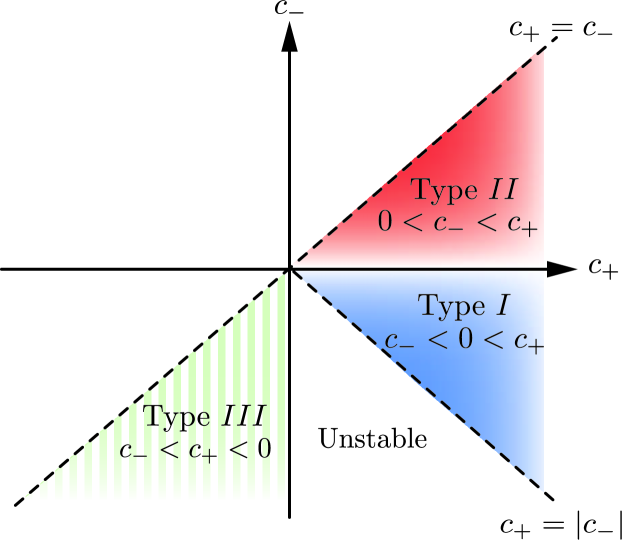
Figure 5: Phase diagram of signal velocities. Sketch of three type of solutions. Type I and Type II are stable with PBC and also on the line. Type III solution is stable only with PBC.

In our analysis below we ignore cases when $c_{\pm}=0$ or $c_{+}=c_{-}$. These cases are interesting by themselves, but have properties that make them undesirable for situations like traffic and other types of flocking. Thus we do not investigate them here. For example when $c_{-}=0$, distances between agents don’t tend to the desired distance $\Delta$, but rather to some value that depends on the initial conditions. If $c_{+}=c_{-}$, which only occurs in Type II solutions, the velocity of the last agent is unbounded as $N$ tends to infinity.

5.1 Type I: Stable, Flockstable, and $c_{-}<0<c_{+}$

When $c_{-}<0<c_{+}$ the solutions resemble the traditional damped wave reflecting between the ends of the flock. The difference in the signal velocities causes the wave to be damped (or magnified) when it reflects in agent $N$. These solutions are called Type I.

For these solutions, it can be shown that the orbit of the last agent [see Figure 2(a)] by the $k$-th amplitude $A_{k}$, the period $T$, and the quotient $|A_{k+1}/A_{k}|$ which we refer to as the attenuation $\alpha$.

Theorem 5.2

Suppose ${\cal S}$ satisfies the conditions of Theorem 5.1. If $c_{-}<0<c_{+}$, then for large enough $N$ and at time scales $t={\cal O}(N)$, the system has Type I solutions characterized by:

$$A_{k}=\frac{-v_{0}N}{c_{+}}\,\left(\frac{c_{-}}{c_{+}}\right)^{k-1}\,,\quad\alpha=\left|\frac{c_{-}}{c_{+}}\right|\,,\quad T=2N\left(\frac{1}{c_{+}}-\frac{1}{c_{-}}\right)\,,$$

where $A_{k}$, $\alpha$, and $T$ are defined above, and $c_{\pm}$ as in Theorem 5.1.

The proof is essentially that of Cantos2014-1 ; Cantos2014-2 and relies on two insights. The first is that the high frequencies die out fast, so that we only need to consider low frequencies (as in the proof of Theorem 5.1). The second is that we replace the physical boundary conditions in ${\cal S}_{N}$ by new boundary conditions to get the correct reflections at the ends, namely a fixed boundary condition at the leader’s end and a free boundary condition at the other end:

$$z_{0}(t)=0\quad\mathrm{and}\quad z_{N}(t)-z_{N-1}(t)=0\,.$$

Because for large $N$ only low frequencies survive, these conditions can be replaced by

$$z_{0}(t)=0\quad\mathrm{and}\quad\frac{\partial}{\partial k}\,z_{k}(t)\big{|}_{k=N}=0\,.$$ (12)

That means that near the leader, a pulse reflects (with opposite sign), and near the free boundary, the traveling pulse is reflected with the same sign and with amplitude multiplied by a factor $|c_{-}/c_{+}|$. The details are written out in Cantos2014-2 .

In order to get strong damping to minimize transients, we want $|c_{-}|<c_{+}$. This means that in the velocity Laplacian, more emphasis should be placed on the upstream (lower labels) information. Such system have asymmetric interactions.

Corollary 5.1

Suppose ${\cal S}$ is asymptotically stable and flock stable. ${\cal S}_{N}$ has solutions of Type I with $|c_{-}|<c_{+}$ if:
(i) $g_{v}\left(\beta_{v,1}+2\beta_{v,2}\right)<0$ and
(ii)$g_{x}\left(4+3\alpha_{x,1}\right)<0$.

Proof: If ${\cal S}$ is asymptotically stable and flock stable, then all ${\cal S}^{*}_{N}$ are stable (by our conjectures). The conditions $c_{-}<0<c_{+}$ and $|c_{-}|<c_{+}$ imply that $c_{-}+c_{+}>0$. This implies (i). Statement (i) together with $c_{-}<0$ implies (ii). ∎

In Figure 6 (parameters are given in the figure) we present typical dynamics of Type I stable system ${\cal S}_{N}$. The characteristics predicted from Theorem 5.2 are $A_{1}=80\,,\alpha=0.4\,,T=560$, and from the simulation we measured $A_{1}=77.2$, $\alpha=0.377$, $T=568$.

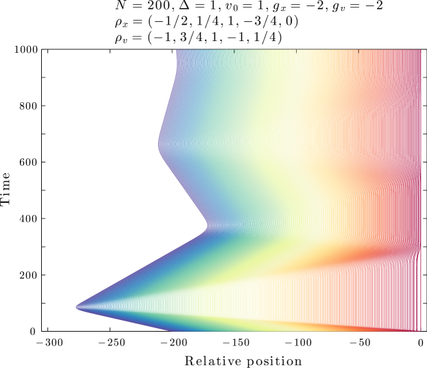
Figure 6: Dynamics of Type I solution. Dynamics of example system ${\cal S}_{N}$ as calculated for $N=200$, $\Delta=1$, $v_{0}=1$, $g_{x}=g_{v}=-2$, $\rho_{x}=(-0.5,0.25,1,-0.75,0)$, $\rho_{v}=(-1,0.75,1,-1,0.25)$ and fixed interaction BC. Each color represent the orbit of one of the $200$ agents.

5.2 Type II: Stable, Flockstable, and $0<c_{-}<c_{+}$

When $0<c_{-}<c_{+}$, that is the signal velocities are both positive, the wave cannot be reflected, because it cannot move with negative velocity. We denote these solutions as Type II or reflectionless waves. It was proved Cantos2014-2 that such solutions cannot occur with nearest neighbor interactions.

Since both signal velocities are positive, there is no reflection possible at $k=N$ agent. Thus the boundary condition at $k=N$ is useless, and we need another boundary condition. We replace Equation (12) by the somewhat counter-intuitive condition:

$$z_{0}(t)=0\quad\mathrm{and}\quad z_{1}(t)-z_{0}(t)=0\,.$$

As before for large $N$ only low frequencies survive, and so these conditions can be replaced by

$$z_{0}(t)=0\quad\mathrm{and}\quad\frac{\partial}{\partial k}\,z_{k}(t)\big{|}_{k=0}=0\,.$$ (13)

Thus we have both a free and a fixed boundary condition at the leader’s end. For Type II, the orbit of the last agent [see Figure 2(b)] can be characterized by the amplitude $A$, the first response time $T_{1}$ and the second response time $T_{2}$.

Theorem 5.3

Suppose ${\cal S}$ satisfies the conditions of Theorem 5.1. If $0<c_{-}<c_{+}$, then for large enough $N$ and at time scales $t={\cal O}(N)$, the system has Type II solutions characterized by:

$$A=\frac{-v_{0}N}{c_{+}}\,,\quad T_{1}=\frac{N}{c_{+}}\,,\quad T_{2}=\frac{N}{c_{-}}\,,$$ (14)

where $A$, $T_{1}$, and $T_{2}$ are as above, and $c_{\pm}$ as in Theorem 5.1.

Proof: $T_{1}$ and $T_{2}$ are the (positive) times at which $z_{N}(t)-z_{0}(t)$ changes velocity. These can be deduced from a Proposition whose reasoning is different enough from earlier work, that we include a sketch of the proof in Appendix C. $A=T_{1}v_{0}$ is the distance traveled by the leader in the time interval $[0,T_{1})$. ∎

Corollary 5.2

Suppose ${\cal S}$ is asymptotically stable and flock stable. ${\cal S}_{N}$ has solutions of Type II (both velocities positive) if:
(i) $g_{v}\left(\beta_{v,1}+2\beta_{v,2}\right)<0$ and
(ii) $0<2g_{x}\left(4+3\alpha_{x,1}\right)<g_{v}^{2}\left(\beta_{v,1}+2\beta_{v,2}\right)^{2}$.

Proof: Similar to the proof of Corollary 5.1. ∎

In Figure 7 we present typical dynamics of Type II stable system ( parameters given in the figure). The characteristics predicted from Theorem 5.3 are $A=43.845$, $T_{1}=43.845$, $T_{2}=456.16$, and from the simulation we measured: $A=43.182$, $T_{1}=43.182$, $T_{2}=453.95$. From the figure it seems that a start signal traveling with velocity $c_{+}$ and a stop signal traveling with velocity $c_{-}$ travel from the leader towards the last agent. A striking aspect of this type of solution is that very briefly after the second response time, the trajectory of the last agent is (almost) exactly in its equilibrium position. Dynamics within such a system can be described as a traveling wave-package which does not reflect in the boundary of the system.

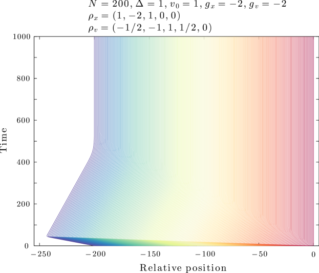
Figure 7: Dynamics of Type II solution. Dynamics of example system ${\cal S}_{N}$ as calculated for $N=200$, $\Delta=1$, $v_{0}=1$, $g_{x}=g_{v}=-2$, $\rho_{x}=(1,-2,1,0,0)$, $\rho_{v}=(-0.5,-1,1,0.5,0)$ and fixed interaction BC. Each color represent the orbit of one of the $200$ agents.

5.3 Type III: $c_{-}<c_{+}<0$

Finally, when $c_{-}<c_{+}<0$, the perturbation which in our set-up starts at the leader, cannot be transmitted to the flock, because only negative signal velocities are available. Thus the system “finds” another non wave-like solution which has very large amplitudes. The only reason for listing this solution in this work at all, is that the system is stable and does have wave-like solutions with negative signal velocities. We call these solutions Type III. As with Type II, these solutions cannot occur with only nearest neighbor interactions.

Corollary 5.3

Suppose ${\cal S}^{*}$ is asymptotically stable. ${\cal S}_{N}$ has solutions of Type III (both velocities negative) if:
(i) $g_{v}\left(\beta_{v,1}+2\beta_{v,2}\right)>0$ and
(ii) $2g_{x}\left(4+3\alpha_{x,1}\right)>0$.

Proof: Similar to the proof of Corollary 5.1. ∎

Within such a setup, on short time scales, the leader simply starts and other agents do not follow him. On time-scales larger than ${\cal O}(N)$, other phenomena may take place. Thus amplitudes will grow faster than ${\cal O}(N)$, and the system is flock unstable or even asymptotically unstable. However, due to the complicated nature of the stability conditions, we do not have a proof of this. In Figure 8 we present a simulation of such a system ( parameters given in the figure). Notice that the amplitudes do not grow linearly with system size.

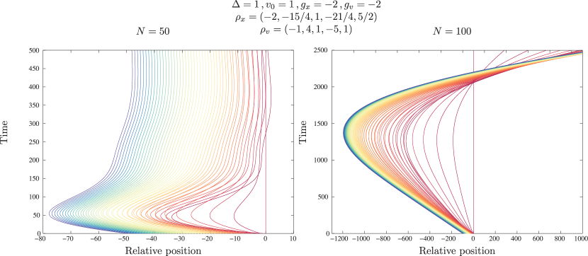
Figure 8: Dynamics of Type III solution. Dynamics of example system ${\cal S}_{N}$ as calculated for $\Delta=1$, $v_{0}=1$, $g_{x}=g_{v}=-2$, $\rho_{x}=(-2,-15/4,1,-21/4,5/2)$, $\rho_{v}=(-1,4,1,-5,1)$, fixed interaction BC $N=50$ (left panel) and $N=100$ (right panel). Each color represent the orbit of one of the $50$ and $100$ agents, respectively.

6 Numerical Tests

As we saw in Section 5, measured values of certain characteristics presented for $N=200$ differ slightly from the predicted ones, given by Theorem 5.2 and Theorem 5.3. This is expected, since our predictions are valid for $N\to\infty$. In order to test our conclusions we performed extensive numerical calculations. We outline our procedure.

First we fixed $g_{x}=g_{v}=-2$ and defined a set $P$ of about $8.6*10^{7}$ ten-tuples
$(g_{x},g_{v},\rho_{x,-2},\rho_{x,-1},\rho_{x,1},\rho_{x,2},\rho_{v,-2},\rho_{v,-1},\rho_{v,1},\rho_{v,1},\rho_{v,2})$ satisfying Equation (3). We call these ten-tuples configurations. From this set of configurations we then selected the set $P_{C}$ that satisfy all the criteria in Remark 4.1. For Type I solutions we impose an additional constraint, namely: $|c_{-}|<c_{+}$ (see Corollary 5.1). Next, from the same ten-tuples of configurations we created the set $P_{S,N}$ that satisfy Definition 3.3 for given $N$. It turns out that for $N$ large enough these sets were identical: $P_{C}=P_{S,N}$ (in our case we had to go up to $N=800$ for a few systems). This strongly suggests that indeed the criteria in Remark 4.1 (plus Corollary 5.1) are a very good indicator of asymptotic stability of the system on the circle.

In order to decrease computation time for large $N$, we imposed a further constraint on $P_{S}$ that selected $500$ configurations of Type I and $500$ configurations of Type II. The constraints were for the period, namely $T\lesssim{\cal O}(10N)$ (Type I), and for the second response time, namely $T_{2}\lesssim{\cal O}(10N)$ (Type II). We ran each of these configurations for $N\in\{25\cdot 2^{n}\}_{n=0}^{n=11}$, that is: for $N$ varying from $25$ to roughly $52,000$. We measure the characteristics directly from numerical simulations and compare them with predictions of Theorem 5.2 and Theorem 5.3. For the numerical work we used the ordinary differential equation solver of the Boost library boostlink ; boostlib in a parallel computing environment.

In Figure 9 we present the relative error=$|measured-predicted|/|predicted|$ of the following quantities: for Type I solutions, the first amplitude $A_{1}$, the period $T$, and the attenuation $\alpha$, and for Type II solutions, the amplitude $A$ and the first and second response times $T_{1}$ and $T_{2}$. We plot both the error average (for $500$ measurements/configurations) and the worst (largest) error. We repeated this experiment for two different types of physical boundary conditions (denoted by fixed interaction and fixed mass (Appendix A) to make sure that these did not make a difference.

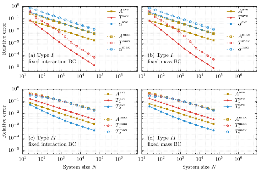
Figure 9: Relative error size scaling. Size $N$ dependence of average and maximal relative error of Type I and Type II solutions for two different boundary condition as calculated for $N=25,\dots,51200$ agents. Notice that the plot has $\log$–$\log$ scale, therefore slope corresponds to the power of the decay.

As is clearly visible in Figure 9, the relative errors decrease as $N$ grows, as is predicted by the theory. Our numerical analysis is consistent with the statement that - with the exception of period $T$ for Type I orbit - the error decreases as ${\cal O}(1/\sqrt{N})$. The error in the period $T$ (for Type I) appears to decrease as ${\cal O}(1/N)$.

Appendix A: The Physical Boundary Conditions

We will introduce two sets of boundary conditions for ${\cal S}_{N}$ (the system on the line). We performed numerics with both types of boundary conditions in order to support our conclusion that for stable and flock stable systems the trajectories are independent of the physical boundary conditions.

Let ${\cal S}_{N}$ be the system in Definition 2.1. In decentralized systems the row sum of the Laplacians equals $0$, that is: $\sum_{j}\rho_{x,j}=\sum_{j}\rho_{v,j}=0$. This implies that for the system ${\cal S}_{N}$, the equations of agents $k=1$, $N-1$, and $N$ have to be modified. In the case of fixed interaction BC the masses, $\rho_{x,0}$ and $\rho_{v,0}$, of the agent are not equal $1$, instead it is the sum of existing interactions. On the other hand, in fixed mass BC we change the interactions of existing agents and keep the central $\rho_{x,0}$ and $\rho_{v,0}$ equal to $1$. Here are the details:

Definition 6.1

(i)

fixed interaction BC:

$$\ddot{z}_{1} = \left(g_{x}\rho_{x,-1}z_{0}+g_{v}\rho_{v,-1}\dot{z}_{0}\right)$$

$$- \left[g_{x}\left(\rho_{x,-1}+\rho_{x,1}+\rho_{x,2}\right)z_{1}+g_{v}\left(\rho_{v,-1}+\rho_{v,1}+\rho_{v,2}\right)\dot{z}_{1}\right]$$

$$+ \sum_{j=1}^{2}\left(g_{x}\rho_{x,j}z_{1+j}+g_{v}\rho_{v,j}\dot{z}_{1+j}\right)\,,$$

$$\ddot{z}_{N-1} = \sum_{j=-2}^{-1}\left(g_{x}\rho_{x,j}z_{N-1+j}+g_{v}\rho_{v,j}\dot{z}_{N-1+j}\right)$$

$$- \left[g_{x}\left(\rho_{x,-2}+\rho_{x,-1}+\rho_{x,1}\right)z_{N-1}+g_{v}\left(\rho_{v,-2}+\rho_{v,-1}+\rho_{v,1}\right)\dot{z}_{N-1}\right]$$

$$+ \left(g_{x}\rho_{x,1}z_{N}+g_{v}\rho_{v,1}\dot{z}_{N}\right)\,,$$

$$\ddot{z}_{N} = \sum_{j=-2}^{-1}\left(g_{x}\rho_{x,j}z_{N+j}+g_{v}\rho_{v,j}\dot{z}_{N+j}\right)$$

$$- \left[g_{x}\left(\rho_{x,-2}+\rho_{x,-1}\right)z_{N}+g_{v}\left(\rho_{v,-2}+\rho_{v,-1}\right)\dot{z}_{N}\right]\,.$$

(ii)

fixed mass BC:

$$\ddot{z}_{1} = \left[g_{x}\left(\rho_{x,-2}+\rho_{x,-1}\right)z_{0}+g_{v}\left(\rho_{v,-2}+\rho_{v,-1}\right)\dot{z}_{0}\right]$$

$$+ \sum_{j=0}^{2}\left(g_{x}\rho_{x,j}z_{1+j}+g_{v}\rho_{v,j}\dot{z}_{1+j}\right)\,,$$

$$\ddot{z}_{N-1} = \sum_{j=-2}^{0}\left(g_{x}\rho_{x,j}z_{N-1+j}+g_{v}\rho_{v,j}\dot{z}_{N-1+j}\right)$$

$$+ \left[g_{x}\left(\rho_{x,1}+\rho_{x,2}\right)z_{N}+g_{v}\left(\rho_{v,1}+\rho_{v,2}\right)\dot{z}_{N}\right]\,,$$

$$\ddot{z}_{N} = \sum_{j=-2}^{0}\left(g_{x}\rho_{x,j}z_{N+j}+g_{v}\rho_{v,j}\dot{z}_{N+j}\right)$$

$$+ \left[g_{x}\left(\rho_{x,1}+\rho_{x,2}\right)z_{N}+g_{v}\left(\rho_{v,1}+\rho_{x,2}\right)\dot{z}_{N}\right]\,.$$

If we use vector notation, the influence of leader on agents $1$ and $2$ is formulated as an external force. Write $z\equiv(z_{1},\;z_{2},\;z_{3},\;\dots\;z_{N}\,)^{T}$ and $\dot{z}\equiv(\dot{z}_{1},\;\dot{z}_{2},\;\dot{z}_{3},\;\dots\;\dot{z}_{N}\,)^{T}$. The equation of motion can be rewritten as a first order system in $2N$ dimensions:

$$\frac{\mathrm{d}}{\mathrm{d}t}\pmatrix{z\cr\dot{z}}=\pmatrix{0&I\cr L_{x}&L_{v}}\pmatrix{z\cr\dot{z}}+F(t)\equiv M_{N}\pmatrix{z\cr\dot{z}}+F(t)\,,$$

Those terms in the full equation of motion that contain $z_{0}$ or $\dot{z}_{0}$ are written as external force. So all components of the external force $F$ are zero except the $N+1$-st and $N+2$-nd. These two components are given by:

$$\pmatrix{g_{x}\rho_{x,-1}z_{0}+g_{v}\rho_{v,-1}\dot{z}_{0}\cr g_{x}\rho_{x,-2}z_{0}+g_{v}\rho_{v,-2}\dot{z}_{0}}\,,$$

if we impose fixed interactions BC, and

$$\pmatrix{g_{x}\left(\rho_{x,-2}+\rho_{x,-1}\right)z_{0}+g_{v}\left(\rho_{v,-2}+\rho_{v,-1}\right)\dot{z}_{0}\cr g_{x}\rho_{x,-2}z_{0}+g_{v}\rho_{v,-2}\dot{z}_{0}}\,,$$

if we impose fixed mass BC.

Appendix B: The Routh-Hurwitz Stability Criteria

The Routh-Hurwitz criterion is a standard strategy to derive a concise set of conditions that is equivalent to the condition that all roots of a given polynomial have negative real parts. In various systems similar to the ones discussed here, this criterion gives good results Cantos2014-1 ; Herman2015 . In our current case the resulting equations are too complicated to give us much information and we only get one more necessary condition for stability that we can use, namely Corollary 6.1. Our discussion is based on Chapter 15, Sections 6, 8, and 13 of Ref. Gantmacher2000 , where more details can be found.

Theorem 6.1

(Routh-Hurwitz) Assume that the determinants given below are nonzero. Given a real polynomial $R=x^{4}+a_{3}x^{3}+a_{2}x^{2}+a_{1}x+a_{0}$, all roots of $R$ have negative real part if and only if all determinants of the upper-left submatrices (the leading principal minors) of:

$$A_{4}\equiv\pmatrix{a_{3}&a_{1}&0&0\cr 1&a_{2}&a_{0}&0\cr 0&a_{3}&a_{1}&0\cr 0&1&a_{2}&a_{0}}\,,$$

are positive. That is: $a_{3}>0$, $a_{0}>0$, $a_{3}a_{2}-a_{1}>0$, and $a_{3}a_{2}a_{1}-a_{3}^{2}a_{0}-a_{1}^{2}>0$.

An equivalent but less well–known set of conditions is given in the following:

Theorem 6.2

(Liénard-Chipart) Assume that the determinants in Theorem 6.1 are nonzero. Given a real polynomial $R=x^{4}+a_{3}x^{3}+a_{2}x^{2}+a_{1}x+a_{0}$, all roots of $R$ have negative real part if and only if $a_{3}>0$, $a_{2}>0$, $a_{0}>0$, and $a_{3}a_{2}a_{1}-a_{3}^{2}a_{0}-a_{1}^{2}>0$.

The characteristic polynomial $Q$ of Equation (9) can be turned into a polynomial with real coefficients

$$R=QQ^{*} \equiv \nu^{4}-2\Re(\lambda_{v})\nu^{3}+\left[|\lambda_{v}|^{2}-2\Re(\lambda_{x})\right]\nu^{2}$$

$$+ 2\left[\Re(\lambda_{x})\Re(\lambda_{v})+\Im(\lambda_{x})\Im(\lambda_{v})\right]\nu+|\lambda_{x}|^{2}\,,$$

by taking its product with its complex conjugate. Clearly, all roots of $Q$ have negative real part if and only if the same is true for $R$. Notice that in each of the two criteria, one of the equations is trivially satisfied, namely $a_{0}>0$ (where we are assuming nondegeneracy). Therefore, in the Routh-Hurwitz case three equations are obtained. The first two are:

$$\Re(\lambda_{v})<0\,,$$ (15)

$$\Re(\lambda_{v})\left[|\lambda_{v}|^{2}-2\Re(\lambda_{x})\right]-\left[\Re(\lambda_{x})\Re(\lambda_{v})+\Im(\lambda_{x})\Im(\lambda_{v})\right]>0\,.$$ (16)

The third inequality we do not utilize, since it is extremely complicated containing fifth order terms. We are left with the above two, which are now necessary conditions for all roots to have negative real part.

Similarly, the Liénard-Chipart stability criterion also gives two necessary conditions for all roots to have negative real part:

$$\Re(\lambda_{v})<0\,,$$ (17)

$$2\Re(\lambda_{x})-|\lambda_{v}|^{2}<0\,.$$ (18)

The third inequality is the same as before and will not be utilized. Since the second inequality of the Liénard-Chipart conditions seems less complicated than the corresponding one of the Routh-Hurwitz conditions, we will continue with the former.

Substituting the expressions for the $\lambda$’s (Lemma 3.1) we get:

$$g_{v}\left[\sum_{j=0}^{2}\alpha_{v,j}\cos(j\phi)\right] < 0\,,$$

$$g_{x}\left[\sum_{j=0}^{2}\alpha_{x,j}\cos(j\phi)\right]-g_{v}^{2}\left\{\left[\sum_{j=0}^{2}\alpha_{v,j}\cos(j\phi)\right]^{2}-\left[\sum_{j=0}^{2}\beta_{v,j}\sin(j\phi)\right]^{2}\right\} < 0\,.$$

These are complicated relations therefore we will use the equivalent relations averaged over $\phi$. The first of these equations was already used in Lemma 4.1. After some calculations we can work out the average over $\phi$ of the second relation. This gives the final necessary condition for all roots to have negative real part.

Corollary 6.1

The following is a necessary condition for the collection ${\cal S}^{*}$ to not be b unstable:

$$g_{x}-g_{v}^{2}\sum_{j=-2}^{2}\rho_{v,j}^{2}\leq 0\,.$$

Appendix C: Analysis of Type II Trajectories

Proposition 6.1

Let $K_{0}>0$ fixed. Suppose that ${\cal S}^{*}$ is stable and that $0<c_{-}<c_{+}$. Suppose further that there are $\alpha\in(0,1)$ and $q>0$ such that $Na_{m}m^{1+q}$ and $Nb_{m}m^{1+q}$ are bounded, and $(2-q)\alpha\leq 1$. Then

$$\lim_{N\rightarrow\infty}\sup_{t\in[0,K_{0}N]}\,|z_{N}(t)-{\overline{z}}_{N}(t)|=0\,.$$

where ${\overline{z}}_{N}(t)$ is given by

$${\overline{z}}_{N}(t)=\left\{\begin{array}[]{cl}-t&t\in\left[0,\frac{N}{c_{+}}\right)\\ \frac{-N}{c_{+}}+\left[\frac{c_{-}}{c_{+}-c_{-}}\right)\left(t-\frac{N}{c_{+}}\right)&t\in\left(\frac{N}{c_{+}},\frac{N}{c_{-}}\right)\\ 0&t\in\left[\frac{N}{c_{-}},\infty\right)\end{array}\right.$$

The signal velocities are as in Theorem 5.1.

Sketch of Proof: We consider the equations of motion for the acceleration $\xi_{k}$ of agent $k$. These are given by the second derivative with respect to time of Definition 2.1. In those equations, the only expression that depends on time is the initial condition of leader. So nothing changes, except that now $\xi_{0}(t)=\delta(t)$ (for $>0$), where $\delta$ is the Dirac function. We replace the Dirac function by a smooth pulse $p(t)$ that enables us to satisfy the decay constraint on the decay of $a_{m}$ and $b_{m}$ but with the condition that $\int\,p(s)\,ds=1$. So now we obtain:

$$\xi_{0}(t)=p(t)$$ (20)

Theorem 5.1 now implies that in ${\cal S}^{*}$ we have

$$\xi_{k}(t)=f_{+}(k-c_{+}t)+f_{-}(k-c_{-}t)$$ (21)

By the periodic boundary conditions conjectures, we see that away from the boundaries the behavior of ${\cal S}$ and ${\cal S}^{*}$ is the same. So we have the above relation from $t=0$ until the signal runs into the boundary at $N$.

Setting $k=0$ in the last equation and comparing with Equation (20) gives

$$p(t)=f_{+}(-c_{+}t)+f_{-}(-c_{-}t)\,.$$ (22)

The second part of Equation (13) then gives:

$$f_{+}^{\prime}(-c_{+}t)+f_{-}^{\prime}(-c_{-}t)=0\,.$$

Integrate with respect to $t$ to get

$$\frac{-1}{c_{+}}f_{+}(-c_{+}t)-\frac{1}{c_{-}}f_{-}(-c_{-}t)=0\quad\Longrightarrow\quad f_{-}(s)=-\frac{c_{-}}{c_{+}}f_{+}\left(\frac{c_{+}}{c_{-}}\,s\right)\,.$$

Substitute this into Equation (22):

$$p(t)=\frac{c_{+}-c_{-}}{c_{+}}f_{+}(-c_{+}t)\quad\Longrightarrow\quad f_{+}(s)=\frac{c_{+}}{c_{+}-c_{-}}p\left(\frac{s}{c_{+}}\right)\,.$$

Now use both of the last equations to eliminate $f_{-}$ and $f_{+}$ from Equation (21):

$$\xi_{k}(t)=\frac{c_{+}}{c_{+}-c_{-}}\,p\left(t-\frac{k}{c_{+}}\right)-\frac{c_{-}}{c_{+}-c_{-}}\,p\left(t-\frac{k}{c_{-}}\right)\,.$$

Now set $k=N$ and integrate twice with respect to time and add a Galilean transformation so that for small positive $t$ we get $z_{N}(t)=-t$. With some rewriting this gives the final result. (As before, to actually prove the remainder indeed tends to zero, one needs the assumption on the decay of the $a_{m}$ and $b_{m}$. This part of the argument is given in Cantos2014-1 .) ∎

References

- [1] F. L. Lewis, H. Zhang, K. Hengster-Movric, and A. Das. Cooperative Control of Multi-Agent Systems: Optimal and Adaptive Design Approaches. Springer Verlag, Germany, 2014.
- [2] S. Backhaus and M. Chertkov. Getting a grip on the electrical grid. Physics Today, 66:42–48, 2013.
- [3] A. E. Motter, S. A. Myers, M. Anghel, and T. Nishikawa. Spontaneous synchrony in power-grid networks. Nature Physics, 9:191–197, 2013.
- [4] B. Bamieh, F. Paganini, and M. Dahleh. Distributed control of spatially invariant systems. IEEE Trans. Autom. Control, 47:1091–1107, 2002.
- [5] D. Cruz, J. McClintock, B. Perteet, O. Orqueda, Y. Cao, and R. Fierro. Decentralized cooperative control: A multivehicle platform for research in networked embedded systems. IEEE Control. Syst. Mag., 27:58–78, 2007.
- [6] M. Defoort, F. Floquet, A. Kokosy, and W. Perruquetti. Sliding-mode formation control for cooperative autonomous mobile robots. IEEE Trans. Ind. Ele., 55:3944–3953, 2008.
- [7] F. Lin, M. Fardad, and M. R. Jovanovic. Optimal control of vehicular formations with nearest neighbor interactions. IEEE Trans. Autom. Control, 57:2203–2218, 2012.
- [8] P. Barooah, P. G. P. Mehta, and J. J. P. Hespanha. Mistuning-based control design to improve closed-loop stability margin of vehicular platoons. IEEE Trans. Autom. Control, 54:2100–2113, 2013.
- [9] I. Herman, D. Martinec, and J. J. P. Veerman. Transients of platoons with asymmetric and different laplacians. Syst. Control Lett., 91:28–35, 2016.
- [10] C. W. Reynolds. Flocks, herds, and schools:a distributed behavioral model. Comput. Graphics, 21:25–34, 1987.
- [11] S. H. Strogatz and I. Stewart. Coupled oscillators and biological synchronization. Sci. Am., 269:102–109, 1993.
- [12] I. D. Couzin, J. Krause, N. R. Franks, and S. A. Levin. Effective leadership and decision-making in animal groups on the move. Nature, 433:513–516, 2005.
- [13] A. Attanasi, A. Cavagna, L. Del Castello, I. Giardina, T. S. Grigera, A. Jelic, S. Melillo, L. Parisi, O. Pohl, E. Shen, and M. Viale. Information transfer and behavioral inertia in starling flocks. Nature Physics, 10:691–696, 2014.
- [14] D. J. G. Pearce, A. M. Miller, G. Rowlands, and M. S. Turner. Role of projection in the control of bird flocks. Proc. Natl. Acad. Sci., 29:10422–10426, 2014.
- [15] W. Ren, R. W. Beard, and E. M. Atkins. A survey of consensus problems in multi-agent coordination. Proceedings of the 2005 American Control Conference, 3:1859–1864, 2005.
- [16] R. Hegselmann and U. Krause. Opinion dynamics and bounded confidence: models, analysis and simulation. J. Artif. Soc. Soc. Simulat., 5(3), 2002.
- [17] N. W. Ashcroft and N. D. Mermin. Solid State Physics. Saunders College, Philadelphia, USA, 1976.
- [18] R. Haberman. Applied Partial Differential Equations with Fourier Series and Boundary Value Problems. Prentice Hall, New Jersey , USA, 4th edition, 2004.
- [19] G. H. Golub and C. F. Van Loan. Matrix Computations. Johns Hopkins University Press, Baltimore, Maryland, United States, 4th edition, 2013.
- [20] C. E. Cantos, D. K. Hammond, and J. J. P. Veerman. Signal velocity in oscillator networks. Eur. Phys. J.-Spec. Top., 225:1115–1126, 2016.
- [21] C. E. Cantos, D. K. Hammond, and J. J. P. Veerman. Transients in the synchronization of oscillator arrays. Eur. Phys. J.-Spec. Top., 225:1199–1209, 2016.
- [22] J. J. P. Veerman. Symmetry and stability of homogeneous flocks (a position paper). Proc. 1st Intern. Conf on Pervasive and Embedded Computing and Communication Systems, Algarve, 21:6, 2010.
- [23] L. N. Trefethen, A. E. Trefethen, S. C. Reddy, and T. A. Driscoll. Hydrodynamic stability without eigenvalues. Science, 261:578–584, 1993.
- [24] L. N. Trefethen. Pseudospectra of linear operators. SIAM Rev., 39:383–406, 1997.
- [25] I. Kra and S. R. Simanca. On circulant matrices. Notices of the Am. Math. Society, 59:368–377, 2012.
- [26] Boost c++ libraries. http://www.boost.org.
- [27] B. Schöing. The Boost C++ Libraries. XML Press, Laguna Hills, USA, 2011.
- [28] F. R. Gantmacher. The Theory of Matrices, volume 2. American Mathematical Society, Providence, USA, 2000.