Energy-Efficient 5G Outdoor-to-Indoor Communication: SUDAS Over Licensed and Unlicensed Spectrum

Abstract

In this paper, we study the joint resource allocation algorithm design for downlink and uplink multicarrier transmission assisted by a shared user equipment (UE)-side distributed antenna system (SUDAS). The proposed SUDAS simultaneously utilizes licensed frequency bands and unlicensed frequency bands, (e.g. millimeter wave bands), to enable a spatial multiplexing gain for single-antenna UEs to improve energy efficiency and system throughput of $5$-th generation (5G) outdoor-to-indoor communication. The design of the UE selection, the time allocation to uplink and downlink, and the transceiver processing matrix is formulated as a non-convex optimization problem for the maximization of the end-to-end system energy efficiency (bits/Joule). The proposed problem formulation takes into account minimum data rate requirements for delay sensitive UEs and the circuit power consumption of all transceivers. In order to design a tractable resource allocation algorithm, we first show that the optimal transmitter precoding and receiver post-processing matrices jointly diagonalize the end-to-end communication channel for both downlink and uplink communication via SUDAS. Subsequently, the matrix optimization problem is converted to an equivalent scalar optimization problem for multiple parallel channels, which is solved by an asymptotically globally optimal iterative algorithm. Besides, we propose a suboptimal algorithm which finds a locally optimal solution of the non-convex optimization problem. Simulation results illustrate that the proposed resource allocation algorithms for SUDAS achieve a significant performance gain in terms of system energy efficiency and spectral efficiency compared to conventional baseline systems by offering multiple parallel data streams for single-antenna UEs. In fact, the proposed SUDAS is able to bridge the gap between the current technology and the high data rate and energy efficiency requirements of 5G outdoor-to-indoor communication systems.

I Introduction

High data rate, high energy efficiency, and ubiquity are basic requirements for $5$-th generation (5G) wireless communication systems. A relevant technique for improving the system throughput for given quality-of-service (QoS) requirements is multiple-input multiple-output (MIMO) [1]–[3], as it provides extra degrees of freedom in the spatial domain which facilitates a trade-off between multiplexing gain and diversity gain. In particular, massive MIMO, which equips the transmitter with a very large number of antennas to serve a comparatively small number of user equipments (UEs), has received considerable interest recently [2, 3]. The high flexibility in resource allocation makes massive MIMO a strong candidate for 5G communication systems. However, state-of-the-art UEs are typically equipped with a small number of receive antennas which limits the spatial multiplexing gain offered by MIMO to individual UEs. On the other hand, the combination of millimeter wave (mmW) and small cells, e.g. femtocells, has been proposed as a core network architecture for 5G indoor communication systems [4, 5] since most mobile data traffic is consumed indoors [6]. The huge free, unlicensed frequency spectrum in the mmW frequency bands appears to be suitable and attractive for providing high speed communication services over short distances in the order of meters. However, the backhauling of the data from the service providers to the small cell base stations (BSs) is a fundamental system bottleneck. In general, the last mile connection from a backbone network to the UEs at homes can only support high data rates if optical fibers are deployed, which is known as fiber-to-the-home (FTTH). Yet, the cost in deploying FTTH for all indoor users is prohibitive. For instance, the cost in equipping every building with FTTH in Germany is estimated to be around $67$ billion Euros [7] which makes high speed small cells not an appealing universal solution for 5G indoor communication systems in terms of implementation cost. Another attractive system architecture for 5G is to combine massive MIMO with mmW communications [8, 9] by using outdoor mmW BSs. However, the high penetration loss of building walls limits the suitability of mmW for outdoor-to-indoor communication scenarios. Thus, additional effective system architecture for outdoor-to-indoor communication is needed.

Distributed antenna systems (DAS) are an existing system architecture on the network side and a special form of MIMO. DAS are able to cover the dead spots in wireless networks, extend service coverage, improve spectral efficiency, and mitigate interference [10, 11]. It is expected that DAS will play an important role in 5G communication systems [12]. Specifically, DAS can realize the potential performance gains of MIMO systems by sharing antennas across different terminals of a communication system to form a virtual MIMO system [13]. Lately, there has been a growing interest in combining orthogonal frequency division multiple access (OFDMA) and DAS to pave the way for the transition of existing communication systems to 5G [14]–[16]. In [14], the authors studied suboptimal resource allocation algorithms for multiuser MIMO-OFDMA systems. In [15], a utility-based low complexity scheduling scheme was proposed for multiuser MIMO-OFDMA systems to strike a balance between system throughput and computational complexity. The optimal subcarrier allocation, power allocation, and bit loading for OFDMA-DAS was investigated in [16]. However, similar to massive MIMO, DAS cannot significantly improve the data rate of individual UE when the UEs are single-antenna devices. Besides, the results in [14]–[16], which are valid for either downlink or uplink communication, may no longer be applicable when joint optimization of downlink and uplink resource usage is considered. Furthermore, the total system throughput in [14]–[16] is not only limited by the number of antennas equipped at the individual UEs, but is also constrained by the system bandwidth which is a very scarce resource in licensed frequency bands. In fact, licensed spectrum is usually located at sub $6$ GHz frequencies which are suitable for long distance communication. On the contrary, the unlicensed frequency spectrum around $60$ GHz offers a large bandwidth of $7$ GHz for wireless communications but is more suitable for short distance communication. The simultaneous utilization of both licensed and unlicensed frequency bands for high rate communication introduces a paradigm shift in system and resource allocation algorithm design due to the related new challenges and opportunities. Yet, the potential system throughput gains of such hybrid systems have not been thoroughly investigated in the literature. Thus, in this work, we study the resource allocation design for hybrid communication systems simultaneously utilizing licensed and unlicensed frequency bands to improve the system performance.

An important requirement for 5G systems is energy efficiency. Over the past decades, the development of wireless communication networks worldwide has triggered an exponential growth in the number of wireless communication devices for real time video teleconferencing, online high definition video streaming, environmental monitoring, and safety management. It is expected that by $2020$, the number of interconnected devices on the planet may reach up to $50$ billion [17]. The related tremendous increase in the number of wireless communication transmitters and receivers has not only led to a huge demand for licensed bandwidth but also for energy. In particular, the escalating energy consumption of electronic circuitries for communication and radio frequency (RF) transmission increases the operation cost of service providers and raises serious environmental concerns due to the produced green house gases. As a result, energy efficiency has become as important as spectral efficiency for evaluation of the performance of the resource utilization in communication networks. A tremendous number of green resource allocation algorithm designs have been proposed in the literature for maximization of the energy efficiency of wireless communication systems [3, 18]–[20]. In [3], joint power allocation and subcarrier allocation was considered for energy-efficient massive MIMO systems. In [18], the energy efficiency of a three-node multiuser MIMO system was studied for the two-hop compress-and-forward relaying protocol. The trade-off between energy efficiency and spectral efficiency in DAS for fair resource allocation in flat fading channels was studied in [19]. Power allocation for energy-efficient DAS was investigated in [20] for frequency-selective channels. However, in [3, 18]–[20], it was assumed that the transmit antennas were deployed by service providers and are connected to a central unit by high cost optical fibers or cables for facilitating simultaneous transmission which may not be feasible in practice. To avoid this problem, unlicensed and licensed frequency bands may be used simultaneously to create a wireless data pipeline for DAS to provide high rate communication services. Nevertheless, the resource allocation algorithm design for such a system architecture has not been investigated in the literature, yet.

In this paper, we propose a shared UE-side distributed antenna system (SUDAS) to assist the outdoor-to-indoor communication in 5G wireless communication systems. In particular, SUDAS simultaneously utilizes licensed and unlicensed frequency bands to facilitate a spatial multiplexing gain for single-antenna transceivers. We formulate the resource allocation algorithm design for SUDAS assisted OFDMA downlink/uplink transmission systems as a non-convex optimization problem. By exploiting the structure of the optimal precoding and post-processing matrices adopted at the BS and the SUDAS, the considered matrix optimization problem is transformed into an equivalent optimization problem with scalar optimization variables. Capitalizing on this transformation, we develop an iterative algorithm which achieves the asymptotically globally optimal performance of the proposed SUDAS for high signal-to-noise ratios (SNRs) and large numbers of subcarriers. Also, the asymptotically optimal algorithm serves as a building block for the design of a suboptimal resource allocation algorithm which achieves a locally optimal solution for the considered problem for arbitrary SNRs.

II SUDAS Assisted OFDMA Network Model

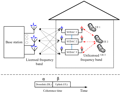
Figure 1: The upper half of the figure illustrates the downlink and uplink communication between a base station (BS) and $K=3$ user equipments (UEs) assisted by $M=3$ SUDACs. The proposed system utilizes a licensed frequency band and an unlicensed frequency band such as the mmW band (e.g. $\sim 60$ GHz). The lower half of the figure depicts the time division duplex (TDD) approach adopted for downlink and uplink communication within a coherence time slot.

II-A SUDAS System Model

We consider a SUDAS assisted OFDMA downlink (DL) and uplink (UL) transmission network which consists of one $N$ antenna BS, a SUDAS, and $K$ single-antenna UEs, cf. Figure 1. The BS is half-duplex and equipped with $N$ antennas for transmitting and receiving signals in a licensed frequency band. The UEs are single-antenna devices receiving and transmitting signals in the unlicensed frequency band. Also, we focus on a wideband multicarrier communication system with $n_{\mathrm{F}}$ orthogonal subcarriers. A SUDAS comprises $M$ shared user equipment (UE)-side distributed antenna components (SUDACs). A SUDAC is a small and cheap device deployed inside a building which simultaneously utilizes both a licensed and an unlicensed frequency band for increasing the DL and UL end-to-end communication data rate. A basic SUDAC is equipped with one antenna for use in a licensed band and one antenna for use in an unlicensed band. We note that the considered single-antenna model for SUDAC can be extended to the case of antenna arrays at the expense of a higher complexity and a more involved notation. Furthermore, a SUDAC is equipped with a mixer to perform frequency up-conversion/down-conversion. For example, for DL communication, the SUDAC receives the signal from the BS in a licensed frequency band, e.g. at $800$ MHz, processes the received signal, and forwards the signal to the UEs in an unlicensed frequency band, e.g. the mmW bands. We note that since the BS-SUDAC link operates in a sub-6 GHz licensed frequency band, it is expected that the associated path loss due to blockage by building walls is much smaller compared to the case where mmW bands were directly used for outdoor-to-indoor communication. Hence, the BS-to-SUDAS channel serves as wireless data pipeline for the SUDAS-to-UE communication channel. Also, since signal reception and transmission at each SUDAC are separated in frequency, cf. Figure 2 and [21], simultaneous signal reception and transmission can be performed in the proposed SUDAS which is not possible for traditional relaying systems due to the limited spectrum availability in the licensed bands. The UL transmission via SUDAS can be performed in a similar manner as the DL transmission and the detailed operation will be discussed in the next section. In practice, a huge bandwidth is available in the unlicensed bands. For instance, there is nearly $7$ GHz unlicensed frequency spectrum available for information transmission in the $57-64$ GHz band (mmW bands).

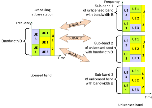
Figure 2: Illustration of signal forwarding from(/to) a licensed band to(/from) different unlicensed frequency sub-bands in the SUDAS.

In this paper, we study the potential system performance gains for outdoor-to-indoor transmission achieved by the proposed SUDAS architecture. In particular, we focus on the case where the SUDACs are installed in electrical wall outlets indoor and can cooperate with each other by sharing channel state information, power, and received signals, e.g. via power line communication links. In other words, for the proposed resource allocation algorithm, joint processing across the SUDACs is assumed to be possible such that the SUDACs can fully exploit the degrees of freedom offered by their antennas. The joint processing architecture of the SUDAS in this paper reveals the maximum potential performance gain of the proposed SUDAS.

Furthermore, we adopt time division duplexing (TDD) to facilitate UL and DL communication for half-duplex UEs and BS. To simplify the following presentation, we assume a normalized unit length time slot whose duration is the coherence time of the channel, i.e., the communication channel is time-invariant within a time slot. Each time slot is divided into two intervals of duration, $\alpha$ and $\beta$, which are allocated for the DL and UL communication, respectively.

II-B SUDAS DL Channel Model

In the DL transmission period $\alpha$, the BS performs spatial multiplexing in the licensed band. The data symbol vector $\mathbf{d}^{[i,k]}_{\mathrm{DL}}\in\mathbb{C}^{N_{\mathrm{S}}\times 1}$ on subcarrier $i\in\{1,\,\ldots,\,n_{F}\}$ for UE $k\in\{1,\,\ldots,\,K\}$ is precoded at the BS as

$$\mathbf{x}^{[i,k]}_{\mathrm{DL}} = \mathbf{P}^{[i,k]}_{\mathrm{DL}}\mathbf{d}^{[i,k]}_{\mathrm{DL}},$$ (1)

where $\mathbf{P}^{[i,k]}_{\mathrm{DL}}\in\mathbb{C}^{N\times N_{\mathrm{S}}}$ is the precoding matrix adopted by the BS on subcarrier $i$ and $\mathbb{C}^{N\times N_{\mathrm{S}}}$ denotes the set of all $N\times N_{\mathrm{S}}$ matrices with complex entries. The signals received on subcarrier $i$ at the $M$ SUDACs for UE $k$ are given by

$$\mathbf{y}^{[i,k]}_{\mathrm{S-DL}} = \mathbf{H}^{[i]}_{\mathrm{B}\rightarrow\mathrm{S}}\mathbf{x}^{[i,k]}_{\mathrm{DL}}+\mathbf{z}^{[i]},$$ (2)

where $\mathbf{y}^{[i,k]}_{\mathrm{S-DL}}=[{y}^{[i,k]}_{\mathrm{S-DL}_{1}},\ldots,{y}^{[i,k]}_{\mathrm{S-DL}_{M}}]^{T}$, ${y}^{[i,k]}_{\mathrm{S-DL}_{m}}$ denotes the received signal at SUDAC $m\in\{1,\ldots,M\}$, and $(\cdot)^{T}$ is the transpose operation. $\mathbf{H}^{[i]}_{\mathrm{B}\rightarrow\mathrm{S}}$ is the $M\times N$ MIMO channel matrix between the BS and the $M$ SUDACs on subcarrier $i$ and captures the joint effects of path loss, shadowing, and multi-path fading. $\mathbf{z}^{[i]}$ is the additive white Gaussian noise (AWGN) vector impairing the $M$ SUDACs in the licensed band on subcarrier $i$ and has a circularly symmetric complex Gaussian (CSCG) distribution ${\cal CN}(\operatorname{\mathbf{0}},\mathbf{\Sigma})$ on subcarrier $i$, where $\operatorname{\mathbf{0}}$ is the mean vector and $\mathbf{\Sigma}$ is the $M\times M$ covariance matrix which is a diagonal matrix with each main diagonal element given by $N_{0}$.

In the unlicensed band, each SUDAC performs orthogonal frequency repetition. In particular, the $M$ SUDACs multiply the received signal vector on subcarrier $i$, $\mathbf{y}^{[i,k]}_{\mathrm{S-DL}}$, by $\mathbf{F}^{[i,k]}_{\mathrm{DL}}\in\mathbb{C}^{M\times M}$ and forward the processed signal vector to UE $k$ on subcarrier $i$ in $M$ different independent frequency sub-bands in the unlicensed spectrum, cf. Figure 2. In other words, different SUDACs forward that received signals in different sub-bands and thereby avoid multiple access interference in the unlicensed spectrum.

The signal received at UE $k$ on subcarrier $i$ from the SUDACs in the $M$ frequency bands, $\mathbf{y}^{[i,k]}_{\mathrm{S}\rightarrow\mathrm{UE}}\in\mathbb{C}^{M\times 1}$ , can be expressed as

$$\mathbf{y}^{[i,k]}_{\mathrm{S}\rightarrow\mathrm{UE}} = \underbrace{\mathbf{H}^{[i,k]}_{\mathrm{S}\rightarrow\mathrm{UE}}\mathbf{F}^{[i,k]}_{\mathrm{DL}}\mathbf{H}^{[i]}_{\mathrm{B}\rightarrow\mathrm{S}}\mathbf{P}^{[i,k]}_{\mathrm{DL}}\mathbf{d}^{[i,k]}_{\mathrm{DL}}}_{\mbox{desired signal}}+\underbrace{\mathbf{H}^{[i,k]}_{\mathrm{S}\rightarrow\mathrm{UE}}\mathbf{F}^{[i,k]}_{\mathrm{DL}}\mathbf{z}^{[i]}}_{\mbox{amplified noise}}+\mathbf{n}^{[i,k]}.$$ (3)

The $m$-th element of vector $\mathbf{y}^{[i,k]}_{\mathrm{S}\rightarrow\mathrm{UE}}$ represents the received DL signal at UE $k$ in the $m$-th unlicensed frequency sub-band. Since the SUDACs forward the DL received signals in different orthogonal frequency bands, $\mathbf{H}^{[i,k]}_{\mathrm{S}\rightarrow\mathrm{UE}}$ is a diagonal matrix with the diagonal elements representing the channel gain between the SUDACs and UE $k$ on subcarrier $i$ in unlicensed sub-band $m$. $\mathbf{n}^{[i,k]}\in\mathbb{C}^{M\times 1}$ is the AWGN vector at UE $k$ on subcarrier $i$ with distribution ${\cal CN}(\operatorname{\mathbf{0}},\mathbf{\Sigma}_{k})$, where $\mathbf{\Sigma}_{k}$ is an ${M\times M}$ diagonal matrix and each main diagonal element is equal to $N_{\mathrm{UE}_{k}}$.

We assume that $M\geq N_{\mathrm{S}}$ and UE $k$ employs a linear receiver for estimating the DL data vector symbol received in the $M$ different sub-bands in the unlicensed band. Hence, the estimated data vector symbol, $\mathbf{\hat{d}}^{[i,k]}_{\mathrm{DL}}\in\mathbb{C}^{N_{\mathrm{S}}\times 1}$, on subcarrier $i$ at UE $k$ is given by

$$\mathbf{\hat{d}}^{[i,k]}_{\mathrm{DL}}=(\mathbf{W}^{[i,k]}_{\mathrm{DL}})^{H}\mathbf{y}^{[i,k]}_{\mathrm{S}\rightarrow\mathrm{UE}},$$ (4)

where $\mathbf{W}^{[i,k]}_{\mathrm{DL}}\in\mathbb{C}^{M\times N_{\mathrm{S}}}$ is a post-processing matrix used for subcarrier $i$ at UE $k$, and $(\cdot)^{H}$ denotes the Hermitian transpose. Without loss of generality, we assume that ${\cal E}\{\mathbf{d}^{[i,k]}_{\mathrm{DL}}(\mathbf{{d}}^{[i,k]}_{\mathrm{DL}})^{H}\}=\mathbf{I}_{N_{\mathrm{S}}}$ where $\mathbf{I}_{N_{\mathrm{S}}}$ is an $N_{\mathrm{S}}\times N_{\mathrm{S}}$ identity matrix and $\cal E\{\cdot\}$ denotes statistical expectation. As a result, the minimum mean square error (MMSE) matrix for data transmission on subcarrier $i$ for UE $k$ via the proposed SUDAS and the optimal MMSE post-processing matrix are given by

$$\mathbf{E}^{[i,k]}_{\mathrm{DL}} = {\cal E}\{(\mathbf{\hat{d}}^{[i,k]}_{\mathrm{DL}}-\mathbf{{d}}^{[i,k]}_{\mathrm{DL}})(\mathbf{\hat{d}}^{[i,k]}_{\mathrm{DL}}-\mathbf{{d}}^{[i,k]}_{\mathrm{DL}})^{H}\}=\Big{[}\mathbf{I}_{N_{\mathrm{S}}}+(\mathbf{\Gamma}^{[i,k]}_{\mathrm{DL}})^{H}(\mathbf{\Theta}^{[i,k]}_{\mathrm{DL}})^{-1}\mathbf{\Gamma}^{[i,k]}_{\mathrm{DL}}\Big{]}^{-1},$$ (5)

$$\mbox{and }\mathbf{W}^{[i,k]}_{\mathrm{DL}} = (\mathbf{\Gamma}^{[i,k]}_{\mathrm{DL}}(\mathbf{\Gamma}^{[i,k]}_{\mathrm{DL}})^{H}+\mathbf{\Theta}^{[i,k]}_{\mathrm{DL}})^{-1}\mathbf{\Gamma}^{[i,k]}_{\mathrm{DL}},$$ (6)

respectively, where $(\cdot)^{-1}$ denotes the matrix inverse, $\mathbf{\Gamma}^{[i,k]}_{\mathrm{DL}}$ is the effective end-to-end channel matrix from the BS to UE $k$ via the SUDAS on subcarrier $i$, and $\mathbf{\Theta}^{[i,k]}_{\mathrm{DL}}$ is the corresponding equivalent noise covariance matrix. These matrices are given by

$$\mathbf{\Gamma}^{[i,k]}_{\mathrm{DL}} = \mathbf{H}^{[i,k]}_{\mathrm{S}\rightarrow\mathrm{UE}}\mathbf{F}^{[i,k]}_{\mathrm{DL}}\mathbf{H}^{[i]}_{\mathrm{B}\rightarrow\mathrm{S}}\mathbf{P}^{[i,k]}_{\mathrm{DL}}\quad\mbox{and}\quad\mathbf{\Theta}^{[i,k]}_{\mathrm{DL}}=\Big{(}\mathbf{H}^{[i,k]}_{\mathrm{S}\rightarrow\mathrm{UE}}\mathbf{F}^{[i,k]}_{\mathrm{DL}}\Big{)}\Big{(}\mathbf{H}^{[i,k]}_{\mathrm{S}\rightarrow\mathrm{UE}}\mathbf{F}^{[i,k]}_{\mathrm{DL}}\Big{)}^{H}+\mathbf{I}_{M}.$$ (7)

Remark 1

The SUDAS concept is fundamentally different from traditional relaying systems which aim at extending service coverage [23, 24]. For DL communication, the SUDAS converts the spatial multiplexing performed at the BS in the licensed band into frequency multiplexing in the unlicensed band to allow single-antenna UEs to decode multiple spatial data streams.

II-C SUDAS UL Channel Model

In the UL transmission period $\beta$, UE $k$ performs frequency multiplexing in the unlicensed band. The data symbol vector $\mathbf{d}^{[i,k]}_{\mathrm{UL}}\in\mathbb{C}^{N_{\mathrm{S}}\times 1}$ on subcarrier $i\in\{1,\,\ldots,\,n_{\mathrm{F}}\}$ from UE $k$ is precoded as

$$\mathbf{x}^{[i,k]}_{\mathrm{UL}}=\mathbf{P}^{[i,k]}_{\mathrm{UL}}\mathbf{d}^{[i,k]}_{\mathrm{UL}},$$ (8)

where $\mathbf{P}^{[i,k]}_{\mathrm{UL}}\in\mathbb{C}^{M\times N_{\mathrm{S}}}$ is the UL precoding matrix adopted by UE $k$ on subcarrier $i$ over the $M$ different frequency sub-bands in the unlicensed spectrum. The signals received on subcarrier $i$ at the $M$ SUDACs for UE $k$ are given by

$$\mathbf{y}^{[i,k]}_{\mathrm{S-UL}} = \mathbf{H}^{[i,k]}_{\mathrm{UE}\rightarrow\mathrm{S}}\mathbf{x}^{[i,k]}_{\mathrm{UL}}+\mathbf{v}^{[i]},$$ (9)

where $\mathbf{y}^{[i,k]}_{\mathrm{S-UL}}=[{y}^{[i,k]}_{\mathrm{S-UL}_{1}}\ldots{y}^{[i,k]}_{\mathrm{S-UL}_{M}}]^{T}$, ${y}^{[i,k]}_{\mathrm{S-UL}_{m}}$ denotes the received signal at SUDAC $m$ in unlicensed frequency sub-band $m\in\{1,\ldots,M\}$, and $\mathbf{v}^{[i]}$ is the AWGN impairing the $M$ SUDACs on subcarrier $i$ in the unlicensed frequency band. $\mathbf{v}^{[i]}$ has distribution ${\cal CN}(\operatorname{\mathbf{0}},\mathbf{\Sigma}_{\mathrm{UL}})$, where $\mathbf{\Sigma}_{\mathrm{UL}}$ is an ${M\times M}$ diagonal matrix and each main diagonal element is equal to $N_{\mathrm{UL}}$. $\mathbf{H}^{[i,k]}_{\mathrm{UE}\rightarrow\mathrm{S}}$ is a diagonal matrix with the main diagonal elements representing the channel gains between UE $k$ and the $M$ SUDACs on subcarrier $i$ in unlicensed sub-band $m$. In fact, the UEs-to-SUDAS channels serve as a short distance wireless data pipeline for the SUDAS-to-BS UL communication.

Each SUDAC forwards the signals received in the unlicensed band in the licensed band to assist the UL communication. In particular, the $M$ SUDACs multiply the received signal vector on subcarrier $i$ by $\mathbf{F}^{[i,k]}_{\mathrm{UL}}\in\mathbb{C}^{M\times M}$ and forward the processed signal vector to the BS on subcarrier $i$ in the licensed spectrum, cf. Figure 2. As a result, the signal received at the BS from UE $k$ on subcarrier $i$ via the SUDAS, $\mathbf{y}^{[i,k]}_{\mathrm{S}\rightarrow\mathrm{B}}\in\mathbb{C}^{N\times 1}$, can be expressed as

$$\mathbf{y}^{[i,k]}_{\mathrm{S}\rightarrow\mathrm{B}} = \underbrace{\mathbf{H}^{[i]}_{\mathrm{S}\rightarrow\mathrm{B}}\mathbf{F}^{[i,k]}_{\mathrm{UL}}\mathbf{H}^{[i,k]}_{\mathrm{UE}\rightarrow\mathrm{S}}\mathbf{P}^{[i,k]}_{\mathrm{UL}}\mathbf{d}^{[i,k]}_{\mathrm{UL}}}_{\mbox{desired signal}}+\underbrace{\mathbf{H}^{[i]}_{\mathrm{S}\rightarrow\mathrm{B}}\mathbf{F}^{[i,k]}_{\mathrm{UL}}\mathbf{z}^{[i]}}_{\mbox{amplified noise}}+\mathbf{n}^{[i,k]}_{\mathrm{B}}.$$ (10)

Matrix $\mathbf{H}^{[i]}_{\mathrm{S}\rightarrow\mathrm{B}}$ is the UL channel between the $M$ SUDACs and the BS on subcarrier $i$, and $\mathbf{n}^{[i,k]}_{\mathrm{B}}$ is the AWGN vector in subcarrier $i$ at the BS with distribution ${\cal CN}(\operatorname{\mathbf{0}},\mathbf{\Sigma}_{\mathrm{B}})$, where $\mathbf{\Sigma}_{\mathrm{B}}$ is an ${M\times M}$ diagonal matrix and each main diagonal element is equal to $N_{\mathrm{B}}$. At the BS, we assume that $N\geq N_{\mathrm{S}}$ and the BS employs a linear receiver for estimating the data vector symbol received from the SUDAS in the licensed band. The estimated data vector symbol, $\mathbf{\hat{d}}^{[i,k]}_{\mathrm{UL}}\in\mathbb{C}^{N_{\mathrm{S}}\times 1}$, on subcarrier $i$ at the BS from UE $k$ is given by

$$\mathbf{\hat{d}}^{[i,k]}_{\mathrm{UL}}=(\mathbf{W}^{[i,k]}_{\mathrm{UL}})^{H}\mathbf{y}^{[i,k]}_{\mathrm{S}\rightarrow\mathrm{B}},$$ (11)

where $\mathbf{W}^{[i,k]}_{\mathrm{UL}}\in\mathbb{C}^{M\times N_{\mathrm{S}}}$ is a post-processing matrix used for subcarrier $i$ at UE $k$. Without loss of generality, we assume that ${\cal E}\{\mathbf{d}^{[i,k]}_{\mathrm{UL}}(\mathbf{{d}}^{[i,k]}_{\mathrm{UL}})^{H}\}=\mathbf{I}_{N_{\mathrm{S}}}$. As a result, the MMSE matrix for data transmission on subcarrier $i$ from UE $k$ to the BS via the SUDAS and the optimal MMSE post-processing matrix are given by

$$\mathbf{E}^{[i,k]}_{\mathrm{UL}} = {\cal E}\{(\mathbf{\hat{d}}^{[i,k]}_{\mathrm{UL}}-\mathbf{{d}}^{[i,k]}_{\mathrm{UL}})(\mathbf{\hat{d}}^{[i,k]}_{\mathrm{UL}}-\mathbf{{d}}^{[i,k]}_{\mathrm{UL}})^{H}\}=\Big{[}\mathbf{I}_{N_{\mathrm{S}}}+(\mathbf{\Gamma}^{[i,k]}_{\mathrm{UL}})^{H}(\mathbf{\Theta}^{[i,k]}_{\mathrm{UL}})^{-1}\mathbf{\Gamma}^{[i,k]}_{\mathrm{UL}}\Big{]}^{-1},$$ (12)

$$\mbox{and }\mathbf{W}^{[i,k]}_{\mathrm{UL}} = (\mathbf{\Gamma}^{[i,k]}_{\mathrm{UL}}(\mathbf{\Gamma}^{[i,k]}_{\mathrm{UL}})^{H}+\mathbf{\Theta}^{[i,k]}_{\mathrm{UL}})^{-1}\mathbf{\Gamma}^{[i,k]}_{\mathrm{UL}},$$ (13)

respectively, where $\mathbf{\Gamma}^{[i,k]}_{\mathrm{UL}}$ is the effective end-to-end channel matrix from UE $k$ to the BS via the SUDAS on subcarrier $i$, and $\mathbf{\Theta}^{[i,k]}_{\mathrm{UL}}$ is the corresponding equivalent noise covariance matrix. These matrices are given by

$$\mathbf{\Gamma}^{[i,k]}_{\mathrm{UL}} = \mathbf{H}^{[i]}_{\mathrm{S}\rightarrow\mathrm{B}}\mathbf{F}^{[i,k]}_{\mathrm{UL}}\mathbf{H}^{[i,k]}_{\mathrm{UE}\rightarrow\mathrm{S}}\mathbf{P}^{[i,k]}_{\mathrm{UL}}\quad\mbox{and}\quad\mathbf{\Theta}^{[i,k]}_{\mathrm{UL}}=\Big{(}\mathbf{H}^{[i,k]}_{\mathrm{UE}\rightarrow\mathrm{S}}\mathbf{F}^{[i,k]}_{\mathrm{UL}}\Big{)}\Big{(}\mathbf{H}^{[i,k]}_{\mathrm{UE}\rightarrow\mathrm{S}}\mathbf{F}^{[i,k]}_{\mathrm{UL}}\Big{)}^{H}+\mathbf{I}_{M}.$$ (14)

Remark 2

Since TDD is adopted and DL and UL transmission occur consecutively within the same coherence time, for resource allocation algorithm design, it is reasonable to assume that channel reciprocity holds, i.e., $\mathbf{H}^{[i,k]}_{\mathrm{UE}\rightarrow\mathrm{S}}=(\mathbf{H}^{[i,k]}_{\mathrm{S}\rightarrow\mathrm{UE}})^{H}$ and $\mathbf{H}^{[i]}_{\mathrm{S}\rightarrow\mathrm{B}}=(\mathbf{H}^{[i]}_{\mathrm{B}\rightarrow\mathrm{S}})^{H}$.

III Problem Formulation

In this section, we first introduce the adopted system performance measure. Then, the design of resource allocation and scheduling is formulated as an optimization problem.

III-A System Throughput

The end-to-end DL and UL achievable data rate on subcarrier $i$ between the BS and UE $k$ via the SUDAS are given by [25]

$$R^{[i,k]}_{\mathrm{DL}}=-\log_{2}\Big{(}\det[\mathbf{E}^{[i,k]}_{\mathrm{DL}}]\Big{)}\quad\mbox{and}\quad R^{[i,k]}_{\mathrm{UL}}=-\log_{2}\Big{(}\det[\mathbf{E}^{[i,k]}_{\mathrm{UL}}]\Big{)},$$ (15)

respectively, where $\det(\cdot)$ is the determinant operation. The DL and UL data rate (bits/s) for UE $k$ can be expressed as

$$\rho^{[k]}_{\mathrm{DL}}=\sum_{i=1}^{n_{\mathrm{F}}}s^{[i,k]}_{\mathrm{DL}}R^{[i,k]}_{\mathrm{UL}}\quad\mbox{and}\quad\rho^{[k]}_{\mathrm{UL}}=\sum_{i=1}^{n_{\mathrm{F}}}s^{[i,k]}_{\mathrm{UL}}R^{[i,k]}_{\mathrm{DL}},$$ (16)

respectively, where $s^{[i,k]}_{\mathrm{DL}}\in\{0,\alpha\}$ and $s^{[i,k]}_{\mathrm{UL}}\in\{0,\beta\}$ are the discrete subcarrier allocation indicators, respectively. In particular, a DL and an UL subcarrier can only be utilized for $\alpha$ and $\beta$ portions of the coherence time, respectively, or not be used at all.

The system throughput is given by

$${\cal U}({\cal P},{\cal S})=\sum_{k=1}^{K}\rho^{[k]}_{\mathrm{DL}}+\sum_{k=1}^{K}\rho^{[k]}_{\mathrm{UL}}\quad[\mbox{bits/s}],$$ (17)

where ${\cal P}=\{\mathbf{P}^{[i,k]}_{\mathrm{DL}},\mathbf{F}^{[i,k]}_{\mathrm{DL}},\mathbf{P}^{[i,k]}_{\mathrm{UL}},\mathbf{F}^{[i,k]}_{\mathrm{UL}}\}$ and ${\cal{S}}=\{s^{[i,k]}_{\mathrm{DL}},s^{[i,k]}_{\mathrm{UL}},\alpha,\beta\}$ are the precoding and subcarrier allocation policies, respectively.

On the other hand, the power consumption of the considered SUDAS assisted communication system consists of seven terms which can be divided into three groups and expressed as

$${\cal U}_{\mathrm{TP}}({\cal P},{\cal S}) = \underbrace{P_{\mathrm{C}_{\mathrm{B}}}+NP_{\mathrm{Ant}_{\mathrm{B}}}+MP_{\mathrm{C}_{\mathrm{SUDAC}}}+KP_{\mathrm{C}_{\mathrm{UE}}}}_{\mbox{System circuit power consumption}}$$ (18a)

$$+ \underbrace{\sum_{k=1}^{K}\sum_{i=1}^{n_{\mathrm{F}}}s^{[i,k]}_{\mathrm{DL}}\varepsilon_{\mathrm{B}}\operatorname{\mathrm{Tr}}\Big{(}\mathbf{P}^{[i,k]}_{\mathrm{DL}}(\mathbf{P}^{[i,k]}_{\mathrm{DL}})^{H}\Big{)}+\sum_{k=1}^{K}\sum_{i=1}^{n_{\mathrm{F}}}s^{[i,k]}_{\mathrm{DL}}\varepsilon_{\mathrm{S}}\operatorname{\mathrm{Tr}}\Big{(}\mathbf{G}^{[i,k]}_{\mathrm{DL}}\Big{)}}_{\mbox{Total DL transmit power consumption}}$$ (18b)

$$+ \underbrace{\sum_{k=1}^{K}\varepsilon_{k}\sum_{i=1}^{n_{\mathrm{F}}}s^{[i,k]}_{\mathrm{UL}}\operatorname{\mathrm{Tr}}\Big{(}\mathbf{P}^{[i,k]}_{\mathrm{UL}}(\mathbf{P}^{[i,k]}_{\mathrm{UL}})^{H}\Big{)}+\sum_{k=1}^{K}\sum_{i=1}^{n_{\mathrm{F}}}s^{[i,k]}_{\mathrm{UL}}\varepsilon_{\mathrm{S}}\operatorname{\mathrm{Tr}}\Big{(}\mathbf{G}^{[i,k]}_{\mathrm{UL}}\Big{)}}_{\mbox{Total UL transmit power consumption}}\quad[\mbox{Joule/s}]$$ (18c)

$$\mbox{where }\quad\mathbf{G}^{[i,k]}_{\mathrm{DL}} = \mathbf{F}^{[i,k]}_{\mathrm{DL}}\Big{(}\mathbf{H}^{[i]}_{\mathrm{B}\rightarrow\mathrm{S}}\mathbf{P}^{[i,k]}_{\mathrm{DL}}(\mathbf{P}^{[i,k]}_{\mathrm{DL}})^{H}(\mathbf{H}^{[i]}_{\mathrm{B}\rightarrow\mathrm{S}})^{H}+\mathbf{I}_{M}\Big{)}(\mathbf{F}^{[i,k]}_{\mathrm{DL}})^{H},$$ (19)

$$\mathbf{G}^{[i,k]}_{\mathrm{UL}} = \mathbf{F}^{[i,k]}_{\mathrm{UL}}\Big{(}\mathbf{H}^{[i,k]}_{\mathrm{UE}\rightarrow\mathrm{S}}\mathbf{P}^{[i,k]}_{\mathrm{UL}}(\mathbf{P}^{[i,k]}_{\mathrm{UL}})^{H}(\mathbf{H}^{[i,k]}_{\mathrm{UE}\rightarrow\mathrm{S}})^{H}+\mathbf{I}_{M}\Big{)}(\mathbf{F}^{[i,k]}_{\mathrm{UL}})^{H},$$ (20)

and $\operatorname{\mathrm{Tr}}(\cdot)$ is the trace operator. The three positive constant terms in (18a), i.e., $P_{\mathrm{C}_{\mathrm{B}}},$ $P_{\mathrm{C}_{\mathrm{SUDAC}}}$, and $P_{\mathrm{C}_{\mathrm{UE}}}$, represent the power dissipation of the circuits [26] for the basic operation of the BS, the SUDAC, and the UE, respectively, and $P_{\mathrm{Ant}_{\mathrm{B}}}$ denotes the circuit power consumption per BS antenna. Equations (18b) and (18c) denote the total DL transmit power consumption and the total UL power consumption, respectively. Specifically, $\operatorname{\mathrm{Tr}}(\mathbf{G}^{[i,k]}_{\mathrm{DL}})$ and $\operatorname{\mathrm{Tr}}(\mathbf{G}^{[i,k]}_{\mathrm{UL}})$ are the DL and UL transmit powers of the SUDAS needed for facilitating the DL and UL communication of UE $k$ in subcarrier $i$, respectively. Similarly, $\operatorname{\mathrm{Tr}}\Big{(}\mathbf{P}^{[i,k]}_{\mathrm{DL}}(\mathbf{P}^{[i,k]}_{\mathrm{DL}})^{H}\Big{)}$ and $\operatorname{\mathrm{Tr}}\Big{(}\mathbf{P}^{[i,k]}_{\mathrm{UL}}(\mathbf{P}^{[i,k]}_{\mathrm{UL}})^{H}\Big{)}$ represent the DL transmit power from the BS to the SUDAS for UE $k$ and the UL transmit power from UE $k$ to the SUDAS in subcarrier $i$, respectively. To capture the power inefficiency of power amplifiers, we introduce linear multiplicative constants $\varepsilon_{\mathrm{B}},\varepsilon_{\mathrm{S}},$ and $\varepsilon_{k}$ for the power radiated by the BS, the SUDAS, and UE $k$ in (18), respectively. For instance, if $\varepsilon_{\mathrm{B}}=4$, then for $1$ Watt of power radiated in the RF, the BS consumes $4$ Watt of power which leads to a power amplifier efficiency of $25\%$.

The energy efficiency of the considered system is defined as the total number of bits exchanged between the BS and the $K$ UEs via the SUDAS per Joule consumed energy:

$${\cal U}_{\mathrm{eff}}({\cal P},{\cal S}) = \frac{{\cal U}({\cal P},{\cal S})}{{\cal U}_{\mathrm{TP}}({\cal P},{\cal S})}\quad[\mbox{bits/Joule}].\vspace*{-4mm}$$ (21)

III-B Problem Formulation

The optimal precoding matrices, ${\cal P}^{*}=\{\mathbf{P}^{[i,k]*}_{\mathrm{DL}},\mathbf{F}^{[i,k]*}_{\mathrm{DL}},\mathbf{P}^{[i,k]*}_{\mathrm{UL}},\mathbf{F}^{[i,k]*}_{\mathrm{UL}}\}$, and the optimal subcarrier allocation policy, ${\cal S}^{*}=\{s^{[i,k]*}_{\mathrm{DL}},s^{[i,k]*}_{\mathrm{UL}},\alpha^{*},\beta^{*}\}$, can be obtained by solving the following optimization problem:

$$\underset{{{\cal P},{\cal S}}}{\operatorname{maximize}}\ \ {\cal U}_{\mathrm{eff}}({\cal P},{\cal S})$$

$$\mathrm{s.t.} \sum_{k=1}^{K}\sum_{i=1}^{n_{\mathrm{F}}}s^{[i,k]}_{\mathrm{DL}}\operatorname{\mathrm{Tr}}\Big{(}\mathbf{P}^{[i,k]}_{\mathrm{DL}}(\mathbf{P}^{[i,k]}_{\mathrm{DL}})^{H}\Big{)}\leq P_{\mathrm{T}},$$ C1: (22)

C2: $$\sum_{k=1}^{K}\sum_{i=1}^{n_{\mathrm{F}}}s^{[i,k]}_{\mathrm{DL}}\operatorname{\mathrm{Tr}}\Big{(}\mathbf{G}^{[i,k]}_{\mathrm{DL}}\Big{)}\leq MP_{\max},$$

C3: $$\sum_{i=1}^{n_{\mathrm{F}}}s^{[i,k]}_{\mathrm{UL}}\operatorname{\mathrm{Tr}}\Big{(}\mathbf{P}^{[i,k]}_{\mathrm{UL}}(\mathbf{P}^{[i,k]}_{\mathrm{UL}})^{H}\Big{)}\leq P_{\max_{k}},\forall k\in\{1,\ldots,K\},$$

C4: $$\sum_{k=1}^{K}\sum_{i=1}^{n_{\mathrm{F}}}s^{[i,k]}_{\mathrm{UL}}\operatorname{\mathrm{Tr}}\Big{(}\mathbf{G}^{[i,k]}_{\mathrm{UL}}\Big{)}\leq P_{\max}^{\mathrm{UL}},$$

C5: $$\rho^{[k]}_{\mathrm{DL}}\geq R^{\mathrm{DL}}_{\min_{k}},\forall k\in{{\cal D}_{\mathrm{DL}}},\quad\mbox{C6: }\rho^{[k]}_{\mathrm{UL}}\geq R^{\mathrm{UL}}_{\min_{k}},\forall k\in{{\cal D}_{\mathrm{UL}}},$$

C7: $$\sum_{i=1}^{n_{\mathrm{F}}}s^{[i,k]}_{\mathrm{DL}}\leq\alpha,\,\forall i,\hskip 46.94704pt\mbox{C8:}\sum_{i=1}^{n_{\mathrm{F}}}s^{[i,k]}_{\mathrm{UL}}\leq\beta,\quad\forall i,$$

C9: $$s^{[i,k]}_{\mathrm{DL}}\in\{0,\alpha\},\forall i,k,\hskip 29.87538pt\mbox{C10: }s^{[i,k]}_{\mathrm{UL}}\in\{0,\beta\},\forall i,k,$$

C11: $$\alpha+\beta\leq 1,\hskip 72.55452pt\mbox{C12: }\alpha,\beta\geq 0.$$

Constants $P_{\mathrm{T}}$ and $MP_{\max}$ in C1 and C2 are the maximum transmit power allowances for the BS and the SUDAS ($M$ SUDACs) for DL transmission, respectively, where $P_{\max}$ is the average transmit power budget for a SUDAC. Similarly, constraints C3 and C4 limit the transmit power for UE $k$ and the SUDAS ($M$ SUDACs) for UL transmission, respectively, where $P_{\max_{k}}$ and $P_{\max}^{\mathrm{UL}}$ are the maximum transmit power budgets of UE $k$ and the SUDAS, respectively. We note that in practice the maximum transmit power allowances for the SUDAS-to-UE, $P_{\max}$, and SUDAS-to-BS, $P_{\max}^{\mathrm{UL}}$, may be different due to different regulations in licensed and unlicensed bands. Sets ${{\cal D}_{\mathrm{DL}}}$ and ${{\cal D}_{\mathrm{UL}}}$ in constraints C5 and C6 denote the set of delay sensitive UEs for DL and UL communication, respectively. In particular, the system has to guarantee a minimum required DL data rate $R^{\mathrm{DL}}_{\min_{k}}$ and UL data rate $R^{\mathrm{UL}}_{\min_{k}}$, if UE $k$ requests delay sensitive services in the DL and UL, respectively. Constraints C7 – C10 are imposed to guarantee that each subcarrier can serve at most one UE for DL and UL communication for fractions of $\alpha$ and $\beta$ of the available time. Constraints C11 and C12 are the boundary conditions for the durations of DL and UL transmission.

IV Resource Allocation Algorithm Design

The considered optimization problem has a non-convex objective function in fractional form. Besides, the precoding matrices $\{\mathbf{P}^{[i,k]}_{\mathrm{DL}},\mathbf{P}^{[i,k]}_{\mathrm{UL}}\}$ and $\{\mathbf{F}^{[i,k]}_{\mathrm{DL}},\mathbf{F}^{[i,k]}_{\mathrm{UL}}\}$ are coupled in (19) and (20) leading to a non-convex feasible solution set in (III-B). Also, constraints C9 and C10 are combinatorial constraints which results in a discontinuity in the solution set. In general, there is no systematic approach for solving non-convex optimization problems optimally. In many cases, an exhaustive search method may be needed to obtain the global optimal solution. Yet, applying such method to our problem will lead to prohibitively high computational complexity since the search space for the optimal solution grows exponentially with respect to $K$ and $n_{\mathrm{F}}$. In order to make the problem tractable, we first transform the objective function in fractional form into an equivalent objective function in subtractive form via fractional programming theory. Subsequently, majorization theory is exploited to obtain the structure of the optimal precoding policy to further simplify the problem. Then, we employ constraint relaxation to handle the binary constraints C9 and C10 to obtain an asymptotically optimal resource allocation algorithm in high SNR regime and for large numbers of subcarriers.

IV-A Transformation of the Optimization Problem

For notational simplicity, we define $\mathcal{F}$ as the set of feasible solutions of the optimization problem in (III-B) spanned by constraints C1 – C12. Without loss of generality, we assume that $\{{\cal P},{\cal S}\}\in\mathcal{F}$ and the solution set $\mathcal{F}$ is non-empty and compact. Then, the maximum energy efficiency of the SUDAS assisted communication, denoted as $\eta_{\mathrm{eff}}^{*}$, is given by

$$\eta_{\mathrm{eff}}^{*}=\frac{{\cal U}({\cal P^{*}},{\cal S^{*}})}{{\cal U}_{\mathrm{TP}}({\cal P^{*}},{\cal S^{*}})}=\underset{\{{\cal P},{\cal S}\}\in\mathcal{F}}{\operatorname{maximize}}\,\frac{{\cal U}({\cal P},{\cal S})}{{\cal U}_{\mathrm{TP}}({\cal P},{\cal S})}.$$ (23)

Now, we introduce the following theorem for handling the optimization problem in (III-B).

Theorem 1

By nonlinear fractional programming theory [27], the resource allocation policy achieves the maximum energy efficiency $\eta_{\mathrm{eff}}^{*}$ if and only if it satisfies

$$\underset{\{{\cal P},{\cal S}\}\in\mathcal{F}}{\operatorname{maximize}}\,\,{\cal U}({\cal P},{\cal S})-\eta_{\mathrm{eff}}^{*}\,{\cal U}_{\mathrm{TP}}({\cal P},{\cal S})={\cal U}({\cal P^{*}},{\cal S^{*}})-\eta_{\mathrm{eff}}^{*}\,{\cal U}_{\mathrm{TP}}({\cal P^{*}},{\cal S^{*}})=0,$$

for ${\cal U}({\cal P},{\cal S})\geq 0$ and ${\cal U}_{\mathrm{TP}}({\cal P},{\cal S})>0$.

 Proof: Please refer to [27] for a proof of Theorem 1. ∎

Theorem 1 states the necessary and sufficient condition for a resource allocation policy to be globally optimal. Hence, for an optimization problem with an objective function in fractional form, there exists an equivalent optimization problem with an objective function in subtractive form, e.g. ${\cal U}({\cal P^{*}},{\cal S^{*}})-\eta_{\mathrm{eff}}^{*}\,{\cal U}_{\mathrm{TP}}({\cal P^{*}},{\cal S^{*}})$ in this paper, such that the same optimal resource allocation policy solves both problems. Therefore, without loss of generality, we can focus on the objective function in equivalent subtractive form to design a resource allocation policy which satisfies Theorem 1 in the sequel.

IV-B Asymptotically Optimal Solution

In this section, we propose an asymptotically optimal iterative algorithm based on the Dinkelbach method [27] for solving (III-B) with an equivalent objective function such that the obtained solution satisfies the conditions stated in Theorem 1. The proposed iterative algorithm is summarized in Table I (on the next page) and the convergence to the optimal energy efficiency is guaranteed if the inner problem (IV-B) is solved in each iteration. Please refer to [27] for a proof of the convergence of the iterative algorithm.

The iterative algorithm is implemented with a repeated loop. In each iteration in the main loop, i.e., lines $3-10$, we solve the following optimization problem for a given parameter $\eta_{\mathrm{eff}}$:

$$\underset{{{\cal P},{\cal S}}}{\operatorname{maximize}}\,\,{\cal U}({\cal P},{\cal S})-\eta_{\mathrm{eff}}{\cal U}_{\mathrm{TP}}({\cal P},{\cal S})$$

$$\mathrm{s.t.}\,\,\mbox{C1 -- C12}.$$ (24)

Table I: Iterative Resource Allocation Algorithm.

Algorithm 1 Iterative Resource Allocation Algorithm

1:  Initialization: $L_{\max}=$ the maximum number of iterations and $\Delta\rightarrow 0$ is the maximum tolerance

2:  Set $\eta_{\mathrm{eff}}=0$ and iteration index $t=0$

3:  repeat {Iteration Process: Main Loop}

4:     For a given $\eta_{\mathrm{eff}}$, solve (IV-B) and obtain an intermediate resource allocation policy $\{{\cal P^{\prime}},{\cal S^{\prime}}\}$

5:     if $\lvert{\cal U}({\cal P^{\prime}},{\cal S^{\prime}})-\eta_{\mathrm{eff}}{\cal U}_{\mathrm{TP}}({\cal P^{\prime}},{\cal S^{\prime}})<\Delta\rvert$ then

6:        $\mbox{Convergence}=\,$true, return $\{{\cal P^{*},\cal S^{*}}\}=\{{\cal P^{\prime},\cal S^{\prime}}\}$ and $\eta_{\mathrm{eff}}^{*}=\frac{{\cal U}({\cal P^{\prime}},{\cal S^{\prime}})}{{\cal U}_{\mathrm{TP}}({\cal P^{\prime}},{\cal S^{\prime}})}$

7:     else

8:        Set $\eta_{\mathrm{eff}}=\frac{{\cal U}({\cal P^{\prime}},{\cal S^{\prime}})}{{\cal U}_{\mathrm{TP}}({\cal P^{\prime}},{\cal S^{\prime}})}$ and $t=t+1$, convergence $=$ false

9:     end if

10:  until Convergence $=$ true or $t=L_{\max}$

Solution of the Main Loop Problem (IV-B)

The transformed objective function is in subtractive form and is parameterized by variable $\eta_{\mathrm{eff}}$. Yet, the transformed problem is still a non-convex optimization problem. We handle the coupled precoding matrices by studying the structure of the optimal precoding matrices for (IV-B). In this context, we define the following matrices to facilitate the subsequent presentation. Using singular value decomposition (SVD), the DL two-hop channel matrices $\mathbf{H}^{[i]}_{\mathrm{B}\rightarrow\mathrm{S}}$ and $\mathbf{H}^{[i,k]}_{\mathrm{S}\rightarrow\mathrm{UE}}$ can be written as

$$\mathbf{H}^{[i]}_{\mathrm{B}\rightarrow\mathrm{S}} = \mathbf{U}^{[i]}_{\mathrm{B}\rightarrow\mathrm{S}}\mathbf{\Lambda}^{[i]}_{\mathrm{B}\rightarrow\mathrm{S}}(\mathbf{V}^{[i]}_{\mathrm{B}\rightarrow\mathrm{S}})^{H}\quad\mbox{and}\quad\mathbf{H}^{[i,k]}_{\mathrm{S}\rightarrow\mathrm{UE}}=\mathbf{U}^{[i,k]}_{\mathrm{S}\rightarrow\mathrm{UE}}\mathbf{\Lambda}^{[i,k]}_{\mathrm{S}\rightarrow\mathrm{UE}}(\mathbf{V}^{[i,k]}_{\mathrm{S}\rightarrow\mathrm{UE}})^{H},$$ (25)

respectively, where $\mathbf{U}^{[i]}_{\mathrm{B}\rightarrow\mathrm{S}}\in{\mathbb{C}^{M\times M}},\mathbf{V}^{[i]}_{\mathrm{B}\rightarrow\mathrm{S}}\in{\mathbb{C}^{N\times N}},\mathbf{U}^{[i,k]}_{\mathrm{S}\rightarrow\mathrm{UE}}\in{\mathbb{C}^{M\times M}},$ and $\mathbf{V}^{[i,k]}_{\mathrm{S}\rightarrow\mathrm{UE}}\in{\mathbb{C}^{M\times M}}$ are unitary matrices. $\mathbf{\Lambda}^{[i]}_{\mathrm{B}\rightarrow\mathrm{S}}$ and $\mathbf{\Lambda}^{[i,k]}_{\mathrm{S}\rightarrow\mathrm{UE}}$ and are $M\times N$ and $M\times M$ matrices with main diagonal element vectors $\Big{[}\sqrt{\gamma_{\mathrm{B}\rightarrow\mathrm{S},1}^{[i]}}\,\sqrt{\gamma_{\mathrm{B}\rightarrow\mathrm{S},2}^{[i]}}\,\ldots\sqrt{\gamma_{\mathrm{B}\rightarrow\mathrm{S},R_{1}}^{[i]}}\Big{]}$ and $\Big{[}\sqrt{\gamma_{\mathrm{S}\rightarrow\mathrm{UE},1}^{[i,k]}}\,\sqrt{\gamma_{\mathrm{S}\rightarrow\mathrm{UE},2}^{[i,k]}}\,$ $\ldots\,\sqrt{\gamma_{\mathrm{S}\rightarrow\mathrm{UE},R_{2}}^{[i,k]}}\Big{]}$, respectively, and all other elements equal to zero. Subscript indices $R_{1}=\operatorname{\mathrm{Rank}}(\mathbf{H}^{[i]}_{\mathrm{B}\rightarrow\mathrm{S}})$ and $R_{2}=\operatorname{\mathrm{Rank}}(\mathbf{H}^{[i,k]}_{\mathrm{S}\rightarrow\mathrm{UE}})$ denote the rank of matrices $\mathbf{H}^{[i]}_{\mathrm{B}\rightarrow\mathrm{S}}$ and $\mathbf{H}^{[i,k]}_{\mathrm{S}\rightarrow\mathrm{UE}}$, respectively. Variables $\gamma_{\mathrm{B}\rightarrow\mathrm{S},n}^{[i]}$ and $\gamma_{\mathrm{S}\rightarrow\mathrm{UE},n}^{[i,k]}$ represent the equivalent channel-to-noise ratio (CNR) on spatial channel $n$ in subcarrier $i$ of the BS-to-SUDAS channel and the SUDAS-to-UE $k$ channel, respectively. Similarly, we can exploit channel reciprocity and apply SVD to the UL two-hop channel matrices which yields

$$\mathbf{H}^{[i]}_{\mathrm{S}\rightarrow\mathrm{B}}=\mathbf{V}^{[i]}_{\mathrm{B}\rightarrow\mathrm{S}}(\mathbf{\Lambda}^{[i]}_{\mathrm{B}\rightarrow\mathrm{S}})^{H}(\mathbf{U}^{[i]}_{\mathrm{B}\rightarrow\mathrm{S}})^{H}\quad\mbox{and}\quad\mathbf{H}^{[i,k]}_{\mathrm{UE}\rightarrow\mathrm{S}}=\mathbf{V}^{[i,k]}_{\mathrm{S}\rightarrow\mathrm{UE}}(\mathbf{\Lambda}^{[i,k]}_{\mathrm{S}\rightarrow\mathrm{UE}})^{H}(\mathbf{U}^{[i,k]}_{\mathrm{S}\rightarrow\mathrm{UE}})^{H}.$$ (26)

We are now ready to introduce the following theorem.

Theorem 2

Assuming that $\operatorname{\mathrm{Rank}}(\mathbf{P}^{[i,k]}_{\mathrm{DL}})=\operatorname{\mathrm{Rank}}(\mathbf{P}^{[i,k]}_{\mathrm{UL}})=\operatorname{\mathrm{Rank}}(\mathbf{F}^{[i,k]}_{\mathrm{DL}})=\operatorname{\mathrm{Rank}}(\mathbf{F}^{[i,k]}_{\mathrm{UL}})=N_{\mathrm{S}}\leq\min\{\operatorname{\mathrm{Rank}}(\mathbf{H}^{[i,k]}_{\mathrm{S}\rightarrow\mathrm{UE}}),\operatorname{\mathrm{Rank}}(\mathbf{H}^{[i]}_{\mathrm{B}\rightarrow\mathrm{S}})\}$, the optimal linear precoding matrices used at the BS and the SUDACs for the maximization problem in (IV-B) jointly diagonalize the DL and UL channels of the BS-SUDAS-UE link on each subcarrier, despite the non-convexity of the objective function. The optimal precoding matrices have the following structure:

$$\mathbf{P}^{[i,k]}_{\mathrm{DL}} = \mathbf{\widetilde{V}}^{[i]}_{\mathrm{B}\rightarrow\mathrm{S}}\mathbf{\Lambda}^{[i,k]}_{\mathrm{B}_{\mathrm{DL}}},\quad\mbox{ }\quad\quad\,\,\,\,\mathbf{F}^{[i,k]}_{\mathrm{DL}}=\mathbf{\widetilde{V}}^{[i,k]}_{\mathrm{S}\rightarrow\mathrm{UE}}\mathbf{\Lambda}^{[i,k]}_{\mathrm{F}_{\mathrm{DL}}}(\mathbf{\widetilde{U}}^{[i,k]}_{\mathrm{B}\rightarrow\mathrm{S}})^{H},$$ (27)

$$\mathbf{P}^{[i,k]}_{\mathrm{UL}} = \mathbf{\widetilde{U}}^{[i]}_{\mathrm{S}\rightarrow\mathrm{UE}}\mathbf{\Lambda}^{[i,k]}_{\mathrm{UE}_{\mathrm{UL}}},\,\,\,\mbox{and}\quad\mathbf{F}^{[i,k]}_{\mathrm{UL}}=\mathbf{\widetilde{U}}^{[i,k]}_{\mathrm{B}\rightarrow\mathrm{S}}\mathbf{\Lambda}^{[i,k]}_{\mathrm{F}_{\mathrm{UL}}}(\mathbf{\widetilde{V}}^{[i,k]}_{\mathrm{S}\rightarrow\mathrm{UE}})^{H},$$ (28)

respectively, where $\mathbf{\widetilde{V}}^{[i]}_{\mathrm{B}\rightarrow\mathrm{S}}$, $\mathbf{\widetilde{V}}^{[i,k]}_{\mathrm{S}\rightarrow\mathrm{UE}}$, and $\mathbf{\widetilde{U}}^{[i,k]}_{\mathrm{B}\rightarrow\mathrm{S}}$ are the $N_{\mathrm{S}}$ rightmost columns of $\mathbf{V}^{[i]}_{\mathrm{B}\rightarrow\mathrm{S}}$, $\mathbf{V}^{[i,k]}_{\mathrm{S}\rightarrow\mathrm{UE}}$, and $\mathbf{U}^{[i,k]}_{\mathrm{B}\rightarrow\mathrm{S}}$, respectively. Matrices $\mathbf{\Lambda}^{[i,k]}_{\mathrm{B}_{\mathrm{DL}}}\in\mathbb{C}^{N_{\mathrm{S}}\times N_{\mathrm{S}}}$, $\mathbf{\Lambda}^{[i,k]}_{\mathrm{F}_{\mathrm{DL}}}\in\mathbb{C}^{N_{\mathrm{S}}\times N_{\mathrm{S}}}$, $\mathbf{\Lambda}^{[i,k]}_{\mathrm{B}_{\mathrm{UL}}}\in\mathbb{C}^{N_{\mathrm{S}}\times N_{\mathrm{S}}}$, and $\mathbf{\Lambda}^{[i,k]}_{\mathrm{F}_{\mathrm{UL}}}\in\mathbb{C}^{N_{\mathrm{S}}\times N_{\mathrm{S}}}$ are diagonal matrices which can be expressed as

$$\mathbf{\Lambda}^{[i,k]}_{\mathrm{B}_{\mathrm{DL}}} = \operatorname{\mathrm{diag}}\Big{(}\sqrt{P_{\mathrm{B}\rightarrow\mathrm{S},1}^{[i,k]}}\,\ldots\,\sqrt{P_{\mathrm{B}\rightarrow\mathrm{S},n}^{[i,k]}}\,\ldots\,\sqrt{P_{\mathrm{B}\rightarrow\mathrm{S},N_{\mathrm{S}}}^{[i,k]}}\Big{)},$$ (29)

$$\mathbf{\Lambda}^{[i,k]}_{\mathrm{F}_{\mathrm{DL}}} = \operatorname{\mathrm{diag}}\Big{(}\sqrt{P_{\mathrm{S}\rightarrow\mathrm{UE},1}^{[i,k]}}\,\ldots\,\sqrt{P_{\mathrm{S}\rightarrow\mathrm{UE},n}^{[i,k]}}\,\ldots\,\sqrt{P_{\mathrm{S}\rightarrow\mathrm{UE},N_{\mathrm{S}}}^{[i,k]}}\Big{)},$$ (30)

$$\mathbf{\Lambda}^{[i,k]}_{\mathrm{UE}_{\mathrm{UL}}} = \operatorname{\mathrm{diag}}\Big{(}\sqrt{P_{\mathrm{UE}\rightarrow\mathrm{S},1}^{[i,k]}}\,\ldots\,\sqrt{P_{\mathrm{UE}\rightarrow\mathrm{S},n}^{[i,k]}}\,\ldots\,\sqrt{P_{\mathrm{UE}\rightarrow\mathrm{S},N_{\mathrm{S}}}^{[i,k]}}\Big{)},\mbox{and}$$ (31)

$$\mathbf{\Lambda}^{[i,k]}_{\mathrm{F}_{\mathrm{UL}}} = \operatorname{\mathrm{diag}}\Big{(}\sqrt{P_{\mathrm{S}\rightarrow\mathrm{B},1}^{[i,k]}}\,\ldots\,\sqrt{P_{\mathrm{S}\rightarrow\mathrm{B},n}^{[i,k]}}\,\ldots\,\sqrt{P_{\mathrm{S}\rightarrow\mathrm{B},N_{\mathrm{S}}}^{[i,k]}}\Big{)},$$ (32)

respectively, where $\operatorname{\mathrm{diag}}(x_{1},\cdots,x_{K})$ denotes a diagonal matrix with the diagonal elements $\{x_{1},\cdots,$ $x_{K}\}$. Scalar optimization variables $P_{\mathrm{B}\rightarrow\mathrm{S},n}^{[i,k]}$, $P_{\mathrm{S}\rightarrow\mathrm{UE},n}^{[i,k]}$, $P_{\mathrm{UE}\rightarrow\mathrm{S},n}^{[i,k]}$, and $P_{\mathrm{S}\rightarrow\mathrm{B},n}^{[i,k]}$ are, respectively, the equivalent transmit powers of the BS-to-SUDAS link, the SUDAS-to-UE link, the UE-to-SUDAS link, and the SUDAS-to-BS link for UE $k$ on spatial channel $n$ and subcarrier $i$.

Proof:

Please refer to the Appendix. ∎

By adopting the optimal precoding matrices provided in Theorem 2, the DL and UL end-to-end channel on subcarrier $i$ is converted into $N_{\mathrm{S}}$ parallel spatial channels. More importantly, the structure of the optimal precoding matrices simplifies the resource allocation algorithm design significantly as the matrix optimization variables can be replaced by equivalent scalar optimization variables. As a result, the achievable rates in DL and UL on subcarrier $i$ from the BS to UE $k$ via the SUDAS in (15) can be simplified as

$$R^{[i,k]}_{\mathrm{DL}} = \sum_{n=1}^{N_{\mathrm{S}}}\log_{2}\Big{(}1+\mathrm{SINR}^{[i,k]}_{\mathrm{DL}_{n}}\Big{)},\,\,\mathrm{SINR}^{[i,k]}_{\mathrm{DL}_{n}}=\frac{\gamma_{\mathrm{B}\rightarrow\mathrm{S},n}^{[i]}P_{\mathrm{B}\rightarrow\mathrm{S},n}^{[i,k]}P_{\mathrm{S}\rightarrow\mathrm{UE},n}^{[i,k]}\gamma_{\mathrm{S}\rightarrow\mathrm{UE},n}^{[i,k]}}{1+\gamma_{\mathrm{B}\rightarrow\mathrm{S},n}^{[i]}P_{\mathrm{B}\rightarrow\mathrm{S},n}^{[i,k]}+P_{\mathrm{S}\rightarrow\mathrm{UE},n}^{[i,k]}\gamma_{\mathrm{S}\rightarrow\mathrm{UE},n}^{[i,k]}},$$ (33)

$$R^{[i,k]}_{\mathrm{UL}} = \sum_{n=1}^{N_{\mathrm{S}}}\log_{2}\Big{(}1+\mathrm{SINR}^{[i,k]}_{\mathrm{UL}_{n}}\Big{)},\,\,\mathrm{SINR}^{[i,k]}_{\mathrm{UL}_{n}}=\frac{\gamma_{\mathrm{S}\rightarrow\mathrm{B},n}^{[i]}P_{\mathrm{S}\rightarrow\mathrm{B},n}^{[i,k]}P_{\mathrm{UE}\rightarrow\mathrm{S},n}^{[i,k]}\gamma_{\mathrm{UE}\rightarrow\mathrm{S},n}^{[i,k]}}{1+\gamma_{\mathrm{S}\rightarrow\mathrm{B},n}^{[i]}P_{\mathrm{S}\rightarrow\mathrm{B},n}^{[i,k]}+P_{\mathrm{UE}\rightarrow\mathrm{S},n}^{[i,k]}\gamma_{\mathrm{UE}\rightarrow\mathrm{S},n}^{[i,k]}},$$ (34)

where $\mathrm{SINR}^{[i,k]}_{\mathrm{DL}_{n}}$ and $\mathrm{SINR}^{[i,k]}_{\mathrm{UL}_{n}}$ are the received signal-to-interference-plus-noise-ratios (SINRs) at UE $k$ and the BS in subcarrier $i$ in spatial subchannel $n\in\{1,\ldots,N_{\mathrm{S}}\}$, respectively. Although the objective function is now a scalar function with respect to the optimization variables, it is still non-convex. To obtain a tractable resource allocation algorithm design, we propose the following objective function approximation. In particular, the end-to-end DL and UL SINRs on subcarrier $i$ for UE $k$ can be approximated, respectively, as

$$\mathrm{SINR}^{[i,k]}_{\mathrm{DL}_{n}} \approx \mathrm{\overline{SINR}}^{[i,k]}_{\mathrm{DL}_{n}}\quad\mbox{and}\quad\mathrm{SINR}^{[i,k]}_{\mathrm{UL}_{n}}\approx\mathrm{\overline{SINR}}^{[i,k]}_{\mathrm{UL}_{n}},\quad\mbox{where}$$ (35)

$$\mathrm{\overline{SINR}}^{[i,k]}_{\mathrm{DL}_{n}} = \frac{\gamma_{\mathrm{B}\rightarrow\mathrm{S},n}^{[i]}P_{\mathrm{B}\rightarrow\mathrm{S},n}^{[i,k]}P_{\mathrm{S}\rightarrow\mathrm{UE},n}^{[i,k]}\gamma_{\mathrm{S}\rightarrow\mathrm{UE},n}^{[i,k]}}{\gamma_{\mathrm{B}\rightarrow\mathrm{S},n}^{[i]}P_{\mathrm{B}\rightarrow\mathrm{S},n}^{[i,k]}+P_{\mathrm{S}\rightarrow\mathrm{UE},n}^{[i,k]}\gamma_{\mathrm{S}\rightarrow\mathrm{UE},n}^{[i,k]}},\,\,\mathrm{\overline{SINR}}^{[i,k]}_{\mathrm{UL}_{n}}=\frac{\gamma_{\mathrm{S}\rightarrow\mathrm{B},n}^{[i]}P_{\mathrm{S}\rightarrow\mathrm{B},n}^{[i,k]}P_{\mathrm{UE}\rightarrow\mathrm{S},n}^{[i,k]}\gamma_{\mathrm{UE}\rightarrow\mathrm{S},n}^{[i,k]}}{\gamma_{\mathrm{S}\rightarrow\mathrm{B},n}^{[i]}P_{\mathrm{S}\rightarrow\mathrm{B},n}^{[i,k]}+P_{\mathrm{UE}\rightarrow\mathrm{S},n}^{[i,k]}\gamma_{\mathrm{UE}\rightarrow\mathrm{S},n}^{[i,k]}}.$$

We note that this approximation is asymptotically tight for high SNR [23, 24].

The next step is to tackle the non-convexity due to combinatorial constraints C9 and C10 in (III-B). To this end, we adopt the time-sharing relaxation approach. In particular, we relax $s^{[i,k]}_{\mathrm{DL}}$ and $s^{[i,k]}_{\mathrm{UL}}$ in constraints C9 and C10 such that they are non-negative real valued optimization variables bounded from above by $\alpha$ and $\beta$, respectively [28], i.e., $0\leq s^{[i,k]}_{\mathrm{DL}}\leq\alpha$ and $0\leq s^{[i,k]}_{\mathrm{UL}}\leq\beta$. It has been shown in [28] that the time-sharing relaxation is asymptotically optimal for a sufficiently large number of subcarriers. Next, we define a set with four auxiliary optimization variables ${\cal\widetilde{P}}=\{\widetilde{P}_{\mathrm{B}\rightarrow\mathrm{S},n}^{[i,k]},\widetilde{P}_{\mathrm{UE}\rightarrow\mathrm{S},n}^{[i,k]},$ $\widetilde{P}_{\mathrm{S}\rightarrow\mathrm{UE},n}^{[i,k]},\widetilde{P}_{\mathrm{S}\rightarrow\mathrm{B},n}^{[i,k]}\}$ and rewrite the transformed objective function in (IV-B) as:

$${\cal U}_{\mathrm{Trans}}({\cal\widetilde{P}},{\cal S})=\sum_{k=1}^{K}\sum_{i=1}^{n_{\mathrm{F}}}\sum_{n=1}^{N_{\mathrm{S}}}\Bigg{\{}s^{[i,k]}_{\mathrm{DL}}\log_{2}\Big{(}1+\frac{\widetilde{\mathrm{{SINR}}}^{[i,k]}_{\mathrm{DL}_{n}}}{s^{[i,k]}_{\mathrm{DL}}}\Big{)}+s^{[i,k]}_{\mathrm{UL}}\log_{2}\Big{(}1+\frac{\widetilde{\mathrm{{SINR}}}^{[i,k]}_{\mathrm{UL}_{n}}}{s^{[i,k]}_{\mathrm{UL}}}\Big{)}\Bigg{\}}$$ (36)

$$-\eta_{\mathrm{eff}}\Big{(}P_{\mathrm{C}_{\mathrm{B}}}+MP_{\mathrm{C}_{\mathrm{SUDAC}}}+KP_{\mathrm{C}_{\mathrm{UE}}}+\sum_{k=1}^{K}\sum_{i=1}^{n_{\mathrm{F}}}\sum_{n=1}^{N_{\mathrm{S}}}\varepsilon_{\mathrm{B}}\widetilde{P}_{\mathrm{B}\rightarrow\mathrm{S},n}^{[i,k]}+\varepsilon_{\mathrm{S}}\widetilde{P}_{\mathrm{S}\rightarrow\mathrm{UE},n}^{[i,k]}+\varepsilon_{k}\widetilde{P}_{\mathrm{UE}\rightarrow\mathrm{S},n}^{[i,k]}+\varepsilon_{\mathrm{S}}\widetilde{P}_{\mathrm{S}\rightarrow\mathrm{B},n}^{[i,k]}\Big{)}$$

where $\widetilde{\mathrm{SINR}}^{[i,k]}_{\mathrm{DL}_{n}}=\overline{\mathrm{{SINR}}}^{[i,k]}_{\mathrm{DL}_{n}}\Big{|}_{\Phi}$ and $\Phi=\Big{\{}\widetilde{P}_{\mathrm{B}\rightarrow\mathrm{S},n}^{[i,k]}=P_{\mathrm{B}\rightarrow\mathrm{S},n}^{[i,k]}s^{[i,k]}_{\mathrm{DL}},\widetilde{P}_{\mathrm{S}\rightarrow\mathrm{UE},n}^{[i,k]}=P_{\mathrm{S}\rightarrow\mathrm{UE},n}^{[i,k]}s^{[i,k]}_{\mathrm{DL}},$ $\widetilde{P}_{\mathrm{UE}\rightarrow\mathrm{S},n}^{[i,k]}=P_{\mathrm{UE}\rightarrow\mathrm{S},n}^{[i,k]}s^{[i,k]}_{\mathrm{UL}},\widetilde{P}_{\mathrm{S}\rightarrow\mathrm{B},n}^{[i,k]}=P_{\mathrm{S}\rightarrow\mathrm{B},n}^{[i,k]}s^{[i,k]}_{\mathrm{UL}}\Big{\}}$. We note that the new auxiliary optimization variables in $\cal\widetilde{P}$ represent the actual transmit energy under the time-sharing condition. As a result, the combinatorial-constraint relaxed problem can be written as:

$$\hskip 28.45274pt\underset{{{\cal\widetilde{P}},}{\cal S}}{\operatorname{maximize}}\ \ {\cal U}_{\mathrm{Trans}}({\cal\widetilde{P}},{\cal S})$$

$$\mathrm{s.t.} \sum_{k=1}^{K}\sum_{i=1}^{n_{\mathrm{F}}}\sum_{n=1}^{N_{\mathrm{S}}}\widetilde{P}_{\mathrm{B}\rightarrow\mathrm{S},n}^{[i,k]}\leq P_{\mathrm{T}},\hskip 34.1433pt\mbox{C2:}\sum_{k=1}^{K}\sum_{i=1}^{n_{\mathrm{F}}}\sum_{n=1}^{N_{\mathrm{S}}}\widetilde{P}_{\mathrm{S}\rightarrow\mathrm{UE},n}^{[i,k]}\leq MP_{\max},$$ C1: (37)

C3: $$\sum_{i=1}^{n_{\mathrm{F}}}\sum_{n=1}^{N_{\mathrm{S}}}\widetilde{P}_{\mathrm{UE}\rightarrow\mathrm{S},n}^{[i,k]}\leq P_{\max_{k}},\forall k,\quad\mbox{C4:}\sum_{k=1}^{K}\sum_{i=1}^{n_{\mathrm{F}}}\sum_{n=1}^{N_{\mathrm{S}}}\widetilde{P}_{\mathrm{S}\rightarrow\mathrm{B},n}^{[i,k]}\leq P_{\max}^{\mathrm{UL}},$$

C5 – C8, $$\mbox{C9: }0\leq s^{[i,k]}_{\mathrm{DL}}\leq\alpha,\forall i,k,\hskip 34.1433pt\mbox{C10: }0\leq s^{[i,k]}_{\mathrm{UL}}\leq\beta,\forall i,k,\mbox{ C11, C12}.$$

Optimization problem (IV-B) is jointly concave with respect to the auxiliary optimization variables $\cal\widetilde{P}$ and $\cal S$. We note that by solving optimization problem (IV-B) for $\widetilde{P}_{\mathrm{B}\rightarrow\mathrm{S}}^{[i,k]}$, $\widetilde{P}_{\mathrm{S}\rightarrow\mathrm{UE},n}^{[i,k]}$, $\widetilde{P}_{\mathrm{UE}\rightarrow\mathrm{S},n}^{[i,k]}$, $\widetilde{P}_{\mathrm{S}\rightarrow\mathrm{B},n}^{[i,k]}$, $s^{[i,k]}_{\mathrm{DL}}$, and $s^{[i,k]}_{\mathrm{UL}}$, we can recover the solution for $P_{\mathrm{B}\rightarrow\mathrm{S},n}^{[i,k]}$, $P_{\mathrm{S}\rightarrow\mathrm{UE},n}^{[i,k]}$, $P_{\mathrm{UE}\rightarrow\mathrm{S},n}^{[i,k]}$, and $P_{\mathrm{S}\rightarrow\mathrm{B},n}^{[i,k]}$. Thus, the solution of (IV-B) is asymptotically optimal with respect to (III-B) for high SNR and a sufficiently large number of subcarriers.

Table II: Iterative Resource Allocation Algorithm for SUDAS Assisted Communication

Algorithm 2 Alternating Optimization

1:  Initialize the maximum number of iterations $L_{\max}$ and a small constant $\kappa\rightarrow 0$

2:  Set iteration index $l=0$ and initialize $\{P_{\mathrm{B}\rightarrow\mathrm{S},n}^{[i,k]}(l),P_{\mathrm{S}\rightarrow\mathrm{UE},n}^{[i,k]}(l),s^{[i,k]}_{\mathrm{DL}}(l)\},\{P_{\mathrm{S}\rightarrow\mathrm{B},n}^{[i,k]}(l),P_{\mathrm{UE}\rightarrow\mathrm{S},n}^{[i,k]}(l),$ $s^{[i,k]}_{\mathrm{UL}}(l)\}$, $\alpha$, $\beta$, and $l=l+1$

3:  repeat {Loop}

4:     For given $P_{\mathrm{S}\rightarrow\mathrm{UE},n}^{[i,k]}(l-1)$ and $\alpha(l)$, solve (IV-B) for $P_{\mathrm{B}\rightarrow\mathrm{S},n}^{[i,k]}$ by using (38) which leads to intermediate power allocation variables $P_{\mathrm{B}\rightarrow\mathrm{S},n}^{[i,k]^{\prime}}$

5:     For given $P_{\mathrm{B}\rightarrow\mathrm{S},n}^{[i,k]^{\prime}}$ and $\alpha(l)$, solve (IV-B) for $P_{\mathrm{S}\rightarrow\mathrm{UE},n}^{[i,k]}$ via equation (40) which leads to intermediate power allocation variables $P_{\mathrm{S}\rightarrow\mathrm{UE},n}^{[i,k]^{\prime}}$

6:     Update the DL subcarrier allocation policy via (44) with $P_{\mathrm{S}\rightarrow\mathrm{UE},n}^{[i,k]}(l-1)$, $P_{\mathrm{B}\rightarrow\mathrm{S},n}^{[i,k]^{\prime}}$, and $\alpha(l)$ to obtain the intermediate DL subcarrier allocation policy $s^{[i,k]^{\prime}}_{\mathrm{DL}}(l)$

7:     For given $P_{\mathrm{S}\rightarrow\mathrm{B},n}^{[i,k]}(l-1)$ and $\beta(l)$, solve (IV-B) for $P_{\mathrm{UE}\rightarrow\mathrm{S},n}^{[i,k]}$ via equation (45) which leads to intermediate power allocation variables $P_{\mathrm{UE}\rightarrow\mathrm{S},n}^{[i,k]^{\prime}}$

8:     For given $P_{\mathrm{UE}\rightarrow\mathrm{S},n}^{[i,k]^{\prime}}$ and $\beta(l)$, solve (IV-B) for $P_{\mathrm{S}\rightarrow\mathrm{B},n}^{[i,k]}$ by using (46) which leads to intermediate power allocation variables $P_{\mathrm{S}\rightarrow\mathrm{B},n}^{[i,k]^{\prime}}$

9:     Update the UL subcarrier allocation policy via (51) with $P_{\mathrm{S}\rightarrow\mathrm{B},n}^{[i,k]}(l-1)$, $P_{\mathrm{UE}\rightarrow\mathrm{S},n}^{[i,k]^{\prime}}$, and $\beta(l)$ to obtain the intermediate UL subcarrier allocation policy $s^{[i,k]^{\prime}}_{\mathrm{UL}}(l)$

10:     Update $\alpha$ and $\beta$ via standard linear programming methods to obtain intermediate solutions of $\alpha^{\prime}$ and $\beta^{\prime}$

11:     if $\lvert P_{\mathrm{S}\rightarrow\mathrm{UE},n}^{[i,k]^{\prime}}-P_{\mathrm{S}\rightarrow\mathrm{UE},n}^{[i,k]}(l-1)\rvert\leq\kappa$ , $\lvert P_{\mathrm{B}\rightarrow\mathrm{S},n}^{[i,k]^{\prime}}-P_{\mathrm{B}\rightarrow\mathrm{S},n}^{[i,k]}(l-1)\rvert\leq\kappa$ , $\lvert s^{[i,k]^{\prime}}_{\mathrm{DL}}-s^{[i,k]}_{\mathrm{DL}}(l-1)\rvert\leq\kappa$, $\lvert P_{\mathrm{UE}\rightarrow\mathrm{S},n}^{[i,k]^{\prime}}-P_{\mathrm{UE}\rightarrow\mathrm{S},n}^{[i,k]}(l-1)\rvert\leq\kappa$ , $\lvert P_{\mathrm{S}\rightarrow\mathrm{B},n}^{[i,k]^{\prime}}-P_{\mathrm{S}\rightarrow\mathrm{B},n}^{[i,k]}(l-1)\rvert\leq\kappa$ , $\lvert s^{[i,k]^{\prime}}_{\mathrm{UL}}-s^{[i,k]}_{\mathrm{UL}}(l-1)\rvert\leq\kappa$$\lvert\alpha^{\prime}-\alpha(l-1)\rvert\leq\kappa$, and $\lvert\beta^{\prime}-\beta(l-1)\rvert\leq\kappa$ then

12:        Convergence = true,  return $\{P_{\mathrm{S}\rightarrow\mathrm{UE},n}^{[i,k]^{\prime}},P_{\mathrm{B}\rightarrow\mathrm{S},n}^{[i,k]^{\prime}},s^{[i,k]^{\prime}}_{\mathrm{DL}},P_{\mathrm{UE}\rightarrow\mathrm{S},n}^{[i,k]^{\prime}},P_{\mathrm{S}\rightarrow\mathrm{B},n}^{[i,k]^{\prime}},s^{[i,k]^{\prime}}_{\mathrm{UL}},\alpha^{\prime},\beta^{\prime}\}$

13:     else

14:        Convergence = false, $P_{\mathrm{S}\rightarrow\mathrm{UE},n}^{[i,k]}(l)=P_{\mathrm{S}\rightarrow\mathrm{UE},n}^{[i,k]^{\prime}},P_{\mathrm{B}\rightarrow\mathrm{S},n}^{[i,k]}(l)=P_{\mathrm{B}\rightarrow\mathrm{S},n}^{[i,k]^{\prime}},s^{[i,k]}_{\mathrm{DL}}(l)=s^{[i,k]^{\prime}}_{\mathrm{DL}},P_{\mathrm{UE}\rightarrow\mathrm{S},n}^{[i,k]}(l)=P_{\mathrm{UE}\rightarrow\mathrm{S},n}^{[i,k]^{\prime}},P_{\mathrm{S}\rightarrow\mathrm{B},n}^{[i,k]}(l)=P_{\mathrm{S}\rightarrow\mathrm{B},n}^{[i,k]^{\prime}},s^{[i,k]}_{\mathrm{UL}}(l)=s^{[i,k]^{\prime}}_{\mathrm{UL}},\alpha(l)=\alpha^{\prime},\beta(l)=\beta^{\prime}$, $l=l+1$

15:     end if

16:  until  $l=L_{\max}$

Now, we propose an algorithm for solving the transformed problem in (IV-B). Although the transformed problem is jointly concave with respect to the optimization variables and can be solved by convex programming solvers, it is difficult to obtain system design insight from a numerical solution. This motivates us to design an iterative resource allocation algorithm which reveals the structure of energy-efficient resource allocation solutions and serves as a building block for the suboptimal algorithm proposed in the next section. The proposed iterative resource allocation algorithm is based on alternating optimization. The algorithm is summarized in Table II and is implemented by a repeated loop. In line 2, we first set the iteration index $l$ to zero and initialize the resource allocation policy. Variables $P_{\mathrm{B}\rightarrow\mathrm{S},n}^{[i,k]}(l),P_{\mathrm{S}\rightarrow\mathrm{UE},n}^{[i,k]}(l),P_{\mathrm{S}\rightarrow\mathrm{B},n}^{[i,k]}(l),P_{\mathrm{UE}\rightarrow\mathrm{S},n}^{[i,k]}(l)$, $s^{[i,k]}_{\mathrm{DL}}(l)$, $s^{[i,k]}_{\mathrm{UL}}(l)$, $\alpha(l)$, and $\beta(l)$ denote the resource allocation policy in the $l$-th iteration. Then, in each iteration, we solve (IV-B), which leads to (38)–(46):

$$P_{\mathrm{B}\rightarrow\mathrm{S},n}^{[i,k]} = \Bigg{[}\frac{\gamma_{\mathrm{S}\rightarrow\mathrm{UE},n}^{[i,k]}P_{\mathrm{S}\rightarrow\mathrm{UE},n}^{[i,k]}\Big{(}\Omega_{\mathrm{B}\rightarrow\mathrm{S},n}^{[i,k]}-\gamma_{\mathrm{S}\rightarrow\mathrm{UE},n}^{[i,k]}P_{\mathrm{S}\rightarrow\mathrm{UE},n}^{[i,k]}-2\Big{)}}{2(\gamma_{\mathrm{B}\rightarrow\mathrm{S},n}^{[i]}\gamma_{\mathrm{S}\rightarrow\mathrm{UE},n}^{[i,k]}P_{\mathrm{S}\rightarrow\mathrm{UE},n}^{[i,k]}+\gamma_{\mathrm{B}\rightarrow\mathrm{S},n}^{[i]})}\Bigg{]}^{+},$$ (38)

$$\Omega_{\mathrm{B}\rightarrow\mathrm{S},n}^{[i,k]} = \frac{\sqrt{4(1+w^{[k]}_{\mathrm{DL}})\gamma_{\mathrm{B}\rightarrow\mathrm{S},n}^{[i]}(1+\gamma_{\mathrm{S}\rightarrow\mathrm{UE},n}^{[i,k]}P_{\mathrm{S}\rightarrow\mathrm{UE},n}^{[i,k]})+(\gamma_{\mathrm{S}\rightarrow\mathrm{UE},n}^{[i,k]})^{2}(\lambda+\eta_{\mathrm{eff}}\varepsilon_{\mathrm{B}})(P_{\mathrm{S}\rightarrow\mathrm{UE},n}^{[i,k]})^{2}\ln(2)}}{\sqrt{\lambda+\eta_{\mathrm{eff}}\varepsilon_{\mathrm{B}}}\sqrt{\ln(2)}},$$ (39)

with $P_{\mathrm{S}\rightarrow\mathrm{UE},n}^{[i,k]}(l-1)$ and $\alpha(l)$ from the last iteration, where $[x]^{+}=\max\{x,0\}$. Then, the obtained intermediate power allocation variable $P_{\mathrm{B}\rightarrow\mathrm{S},n}^{[i,k]}$ is used as an input for solving (IV-B) for $P_{\mathrm{S}\rightarrow\mathrm{UE},n}^{[i,k]}$ via the following equations:

$$P_{\mathrm{S}\rightarrow\mathrm{UE},n}^{[i,k]} = \Bigg{[}\frac{\gamma_{\mathrm{B}\rightarrow\mathrm{S},n}^{[i]}P_{\mathrm{B}\rightarrow\mathrm{S},n}^{[i,k]}\left(\Omega_{\mathrm{S}\rightarrow\mathrm{UE},n}^{[i,k]}-\gamma_{\mathrm{B}\rightarrow\mathrm{S},n}^{[i]}P_{\mathrm{B}\rightarrow\mathrm{S},n}^{[i,k]}-2\right)}{2(\gamma_{\mathrm{B}\rightarrow\mathrm{S},n}^{[i]}\gamma_{\mathrm{S}\rightarrow\mathrm{UE},n}^{[i,k]}P_{\mathrm{B}\rightarrow\mathrm{S},n}^{[i,k]}+\gamma_{\mathrm{S}\rightarrow\mathrm{UE},n}^{[i,k]})}\Bigg{]}^{+},$$ (40)

$$\Omega_{\mathrm{S}\rightarrow\mathrm{UE},n}^{[i,k]} = \frac{\sqrt{(\gamma_{\mathrm{B}\rightarrow\mathrm{S},n}^{[i]})^{2}(\delta+\eta_{\mathrm{eff}}\varepsilon_{\mathrm{S}})(P_{\mathrm{B}\rightarrow\mathrm{S},n}^{[i,k]})^{2}\ln(2)+(\gamma_{\mathrm{B}\rightarrow\mathrm{S},n}^{[i]}P_{\mathrm{B}\rightarrow\mathrm{S},n}^{[i,k]}+1)4(1+w^{[k]}_{\mathrm{DL}})\gamma_{\mathrm{S}\rightarrow\mathrm{UE},n}^{[i,k]}}}{\sqrt{\delta+\eta_{\mathrm{eff}}\varepsilon_{\mathrm{S}}}\sqrt{\ln(2)}}.$$ (41)

(38)–(46) are obtained by standard convex optimization techniques. $\lambda$ and $\delta$ in (38) and (40) are the Lagrange multipliers for constraints C1 and C2 in (IV-B), respectively. In particular, $\lambda$ and $\delta$ are monotonically decreasing with respect to $P_{\mathrm{B}\rightarrow\mathrm{S},n}^{[i,k]}$ and $P_{\mathrm{S}\rightarrow\mathrm{UE},n}^{[i,k]}$, respectively, and control the transmit power at the BS and the SUDAS to satisfy constraints C1 and C2, respectively. Besides, $w^{[k]}_{\mathrm{DL}}\geq 0$ is the Lagrange multiplier associated with the minimum required DL data rate constraint C5 for delay sensitive UE $k$. The optimal values of $\lambda$, $\delta$, and $w^{[k]}_{\mathrm{DL}}$ in each iteration can be found by a standard gradient algorithm such that constraints C1, C2, and C4 in (IV-B) are satisfied. Variable $\eta_{\mathrm{eff}}\geq 0$ generated by the Dinkelbach method prevents unnecessary energy expenditures by reducing the values of $\Omega_{\mathrm{B}\rightarrow\mathrm{S},n}^{[i,k]}$ and $\Omega_{\mathrm{S}\rightarrow\mathrm{UE},n}^{[i,k]}$ in (39) and (41), respectively. Besides, the power allocation strategy in (38) and (40) is analogous to the water-filling solution in traditional single-hop communication systems. In particular, $\Omega_{\mathrm{S}\rightarrow\mathrm{UE},n}^{[i,k]}$ and $\Omega_{\mathrm{B}\rightarrow\mathrm{S},n}^{[i,k]}$ act as water levels for controlling the allocated power. Interestingly, the water level in the power allocation for the BS-to-SUDAS link depends on the associated channel gain which is different from the power allocation in non-SUDAS assisted communication [15, 16]. Furthermore, it can be seen from (39) and (41) that the water levels of different users can be different. Specifically, if the end-to-end channel gains of two users are the same, to satisfy the data rate requirement, the water level of the delay-sensitive user is generally higher than that of the non-delay sensitive user.

After obtaining the intermediate DL power allocation policy, cf. lines 4, 5, we update the DL subcarrier allocation, cf. line 6, as:

$$s^{[i,k]}_{\mathrm{DL}} = \left\{\begin{array}[]{rl}\alpha&\mbox{if $k=\arg\underset{t\in\{1,\ldots,K\}}{\max}\,(1+w^{[t]}_{\mathrm{DL}})\Big{(}\sum_{n=1}^{N}\log_{2}\Big{(}1+\mathrm{\overline{SINR}}^{[i,t]}_{\mathrm{DL}_{n}}\Big{)}-\frac{\mathrm{\overline{SINR}}^{[i,t]}_{\mathrm{DL}_{n}}}{1+\mathrm{\overline{SINR}}^{[i,t]}_{\mathrm{DL}_{n}}}\Big{)}$ }\\ 0&\mbox{ otherwise}\end{array}\right..$$ (44)

Here, $\mathrm{\overline{SINR}}^{[i,k]}_{\mathrm{DL}_{n}}$ is obtained by substituting the intermediate solution of $P_{\mathrm{B}\rightarrow\mathrm{S},n}^{[i,k]^{\prime}}$ and $P_{\mathrm{S}\rightarrow\mathrm{UE},n}^{[i,k]^{\prime}}$, i.e., (38) and (40), into (35) in the $l$-th iteration. We note that the optimal value of $s^{[i,k]}_{\mathrm{DL}}$ of the relaxed problem is a discrete value, cf. (44), i.e., the constraint relaxation is tight.

Similarly, we optimize the UL power allocation variables, $P_{\mathrm{UE}\rightarrow\mathrm{S},n}^{[i,k]}$ and $P_{\mathrm{S}\rightarrow\mathrm{B},n}^{[i,k]}$, sequentially, cf. lines 7, 8, via the following equations:

$$P_{\mathrm{UE}\rightarrow\mathrm{S},n}^{[i,k]} = \Bigg{[}\frac{\gamma_{\mathrm{S}\rightarrow\mathrm{B},n}^{[i]}P_{\mathrm{S}\rightarrow\mathrm{B},n}^{[i,k]}\left(\Omega_{\mathrm{UE}\rightarrow\mathrm{S},n}^{[i,k]}-\gamma_{\mathrm{S}\rightarrow\mathrm{B},n}^{[i]}P_{\mathrm{S}\rightarrow\mathrm{B},n}^{[i,k]}-2\right)}{2(\gamma_{\mathrm{S}\rightarrow\mathrm{B},n}^{[i]}\gamma_{\mathrm{UE}\rightarrow\mathrm{S},n}^{[i,k]}P_{\mathrm{S}\rightarrow\mathrm{B},n}^{[i,k]}+\gamma_{\mathrm{UE}\rightarrow\mathrm{S},n}^{[i,k]})}\Bigg{]}^{+},$$ (45)

$$P_{\mathrm{S}\rightarrow\mathrm{B},n}^{[i,k]} = \Bigg{[}\frac{\gamma_{\mathrm{UE}\rightarrow\mathrm{S},n}^{[i,k]}P_{\mathrm{UE}\rightarrow\mathrm{S},n}^{[i,k]}\left(\Omega_{\mathrm{S}\rightarrow\mathrm{B},n}^{[i,k]}-\gamma_{\mathrm{UE}\rightarrow\mathrm{S},n}^{[i,k]}P_{\mathrm{UE}\rightarrow\mathrm{S},n}^{[i,k]}-2\right)}{2(\gamma_{\mathrm{S}\rightarrow\mathrm{B},n}^{[i]}\gamma_{\mathrm{UE}\rightarrow\mathrm{S},n}^{[i,k]}P_{\mathrm{UE}\rightarrow\mathrm{S},n}^{[i,k]}+\gamma_{\mathrm{S}\rightarrow\mathrm{B},n}^{[i]})}\Bigg{]}^{+},$$ (46)

respectively, where

$$\Omega_{\mathrm{UE}\rightarrow\mathrm{S},n}^{[i,k]} = \frac{\sqrt{(\gamma_{\mathrm{S}\rightarrow\mathrm{B},n}^{[i]})^{2}(\psi_{k}+\eta_{\mathrm{eff}}\varepsilon_{k})(P_{\mathrm{S}\rightarrow\mathrm{B},n}^{[i,k]})^{2}\ln(2)+(\gamma_{\mathrm{S}\rightarrow\mathrm{B},n}^{[i]}P_{\mathrm{S}\rightarrow\mathrm{B},n}^{[i,k]}+1)4(1+w^{[k]}_{\mathrm{UL}})\gamma_{\mathrm{UE}\rightarrow\mathrm{S},n}^{[i,k]}}}{\sqrt{\psi_{k}+\eta_{\mathrm{eff}}\varepsilon_{k}}\sqrt{\ln(2)}},$$ (47)

$$\Omega_{\mathrm{S}\rightarrow\mathrm{B},n}^{[i,k]} = \frac{\sqrt{4(1+w^{[k]}_{\mathrm{UL}})\gamma_{\mathrm{S}\rightarrow\mathrm{B},n}^{[i]}(1+\gamma_{\mathrm{UE}\rightarrow\mathrm{S},n}^{[i,k]}P_{\mathrm{UE}\rightarrow\mathrm{S},n}^{[i,k]})+(\gamma_{\mathrm{UE}\rightarrow\mathrm{S},n}^{[i,k]})^{2}(\phi+\eta_{\mathrm{eff}}\varepsilon_{\mathrm{S}})(P_{\mathrm{UE}\rightarrow\mathrm{S},n}^{[i,k]})^{2}\ln(2)}}{\sqrt{\phi+\eta_{\mathrm{eff}}\varepsilon_{\mathrm{S}}}\sqrt{\ln(2)}}.$$ (48)

$\psi_{k}$ and $\phi$ in (47) and (48) are the Lagrange multipliers with respect to power consumption constraints C3 and C4 in (IV-B), respectively. Besides, $w^{[k]}_{\mathrm{UL}}$ is the Lagrange multiplier associated with the minimum required UL data rate constraint C6 for delay sensitive UE $k$. The optimal values of $\psi_{k}$, $\phi$, and $w^{[k]}_{\mathrm{UL}}$ in each iteration can be easily obtained again with a standard gradient algorithm such that constraints C3, C4, and C6 in (IV-B) are satisfied.

Then, we update the UL subcarrier allocation policy $s^{[i,k]}_{\mathrm{UL}}$ via

$$s^{[i,k]}_{\mathrm{UL}} = \left\{\begin{array}[]{rl}\beta&\mbox{if $k=\arg\underset{t\in\{1,\ldots,K\}}{\max}\,(1+w^{[t]}_{\mathrm{UL}})\Big{(}\sum_{n=1}^{N}\log_{2}\Big{(}1+\mathrm{\overline{SINR}}^{[i,t]}_{\mathrm{UL}_{n}}\Big{)}-\frac{\mathrm{\overline{SINR}}^{[i,t]}_{\mathrm{UL}_{n}}}{1+\mathrm{\overline{SINR}}^{[i,t]}_{\mathrm{UL}_{n}}}\Big{)}$ }\\ 0&\mbox{ otherwise}\end{array}\right..$$ (51)

where $\mathrm{\overline{SINR}}^{[i,k]}_{\mathrm{UL}_{n}}$ is obtained by substituting the intermediate solutions for $P_{\mathrm{S}\rightarrow\mathrm{B},n}^{[i,k]^{\prime}}$ and $P_{\mathrm{UE}\rightarrow\mathrm{S},n}^{[i,k]^{\prime}}$, i.e., (45) and (46), into (35) in the $l$-th iteration. Again, the constraint relaxation is tight.

Subsequently, for a given UL and DL power allocation policy and given $s^{[i,k]}_{\mathrm{DL}}$ and $s^{[i,k]}_{\mathrm{UL}}$, the optimization problem is a linear programming with respect to $\alpha$ and $\beta$. Thus, we can update $\alpha$ and $\beta$ via standard linear programming methods to obtain intermediate solutions for $\alpha^{\prime}$ and $\beta^{\prime}$. Then, the overall procedure is repeated iteratively until we reach the maximum number of iterations or convergence is achieved. We note that for a sufficient number of iterations, the convergence to the optimal solution of (IV-B) is guaranteed since (IV-B) is jointly concave with respect to the optimization variables [30]. Besides, the proposed algorithm has a polynomial time computational complexity.

IV-C Suboptimal Solution

In the last section, we proposed an asymptotically globally optimal algorithm based on the high SNR assumption. In this section, we propose a suboptimal resource allocation algorithm which achieves a local optimal solution of (III-B) for arbitrary SNR values. Similar to the asymptotically optimal solution, we apply Theorem 1, Theorem 2, and Algorithm 1 to simplify the power allocation and subcarrier allocation. In particular, the DL and UL data rates of UE $k$ on subcarrier $i$ are given by (33) and (34), respectively. It can be observed that (33) and (34) are concave functions with respect to $P_{\mathrm{B}\rightarrow\mathrm{S},n}^{[i,k]}$, $P_{\mathrm{S}\rightarrow\mathrm{B},n}^{[i,k]}$, $P_{\mathrm{S}\rightarrow\mathrm{UE},n}^{[i,k]}$, and $P_{\mathrm{UE}\rightarrow\mathrm{S},n}^{[i,k]}$ individually, when the other variables are fixed. Thus, we can apply alternating optimization to obtain a local optimal solution [30] of (III-B). We note that unlike the proposed asymptotically optimal scheme, the high SNR assumption is not required to convexify the problem. The suboptimal solution can be obtained by Algorithm 2 in Table II, but now, we update the power allocation variables, i.e., lines 4, 5, 7, 8, in Algorithm 2, by using the following equations:

$$P_{\mathrm{B}\rightarrow\mathrm{S},n}^{[i,k]} = \frac{1}{\gamma_{\mathrm{B}\rightarrow\mathrm{S},n}^{[i]}}\Bigg{[}\frac{P_{\mathrm{S}\rightarrow\mathrm{UE},n}^{[i,k]}\gamma_{\mathrm{S}\rightarrow\mathrm{UE},n}^{[i,k]}}{2}\Bigg{(}\sqrt{1+\frac{4\gamma_{\mathrm{B}\rightarrow\mathrm{S},n}^{[i]}(1+w^{[k]}_{\mathrm{DL}})}{\gamma_{\mathrm{S}\rightarrow\mathrm{UE},n}^{[i,k]}P_{\mathrm{S}\rightarrow\mathrm{UE},n}^{[i,k]}\ln(2)(\lambda+\eta_{\mathrm{eff}}\varepsilon_{\mathrm{B}})}}-1\Bigg{)}-1\Bigg{]}^{+},$$ (52)

$$P_{\mathrm{S}\rightarrow\mathrm{UE},n}^{[i,k]} = \frac{1}{\gamma_{\mathrm{S}\rightarrow\mathrm{UE},n}^{[i,k]}}\Bigg{[}\frac{P_{\mathrm{B}\rightarrow\mathrm{S},n}^{[i,k]}\gamma_{\mathrm{B}\rightarrow\mathrm{S},n}^{[i]}}{2}\Bigg{(}\sqrt{1+\frac{4\gamma_{\mathrm{S}\rightarrow\mathrm{UE},n}^{[i,k]}(1+w^{[k]}_{\mathrm{DL}})}{\gamma_{\mathrm{B}\rightarrow\mathrm{S},n}^{[i]}P_{\mathrm{B}\rightarrow\mathrm{S},n}^{[i,k]}\ln(2)(\delta+\eta_{\mathrm{eff}}\varepsilon_{\mathrm{S}})}}-1\Bigg{)}-1\Bigg{]}^{+},$$ (53)

$$P_{\mathrm{S}\rightarrow\mathrm{B},n}^{[i,k]} = \frac{1}{\gamma_{\mathrm{S}\rightarrow\mathrm{B},n}^{[i]}}\Bigg{[}\frac{P_{\mathrm{UE}\rightarrow\mathrm{S},n}^{[i,k]}\gamma_{\mathrm{UE}\rightarrow\mathrm{S},n}^{[i,k]}}{2}\Bigg{(}\sqrt{1+\frac{4\gamma_{\mathrm{S}\rightarrow\mathrm{B},n}^{[i]}(1+w^{[k]}_{\mathrm{UL}})}{\gamma_{\mathrm{UE}\rightarrow\mathrm{S},n}^{[i,k]}P_{\mathrm{UE}\rightarrow\mathrm{S},n}^{[i,k]}\ln(2)(\phi+\eta_{\mathrm{eff}}\varepsilon_{\mathrm{S}})}}-1\Bigg{)}-1\Bigg{]}^{+},$$ (54)

$$P_{\mathrm{UE}\rightarrow\mathrm{S},n}^{[i,k]} = \frac{1}{\gamma_{\mathrm{UE}\rightarrow\mathrm{S},n}^{[i,k]}}\Bigg{[}\frac{P_{\mathrm{S}\rightarrow\mathrm{B},n}^{[i,k]}\gamma_{\mathrm{S}\rightarrow\mathrm{B},n}^{[i]}}{2}\Bigg{(}\sqrt{1+\frac{4\gamma_{\mathrm{UE}\rightarrow\mathrm{S},n}^{[i,k]}(1+w^{[k]}_{\mathrm{UL}})}{\gamma_{\mathrm{S}\rightarrow\mathrm{B},n}^{[i]}P_{\mathrm{S}\rightarrow\mathrm{B},n}^{[i,k]}\ln(2)(\psi_{k}+\eta_{\mathrm{eff}}\varepsilon_{k})}}-1\Bigg{)}-1\Bigg{]}^{+},$$ (55)

which are obtained by applying standard optimization technique [24]. Besides, the subcarrier allocation policies for DL and UL are still given by (44) and (51), respectively, except that we replace $\mathrm{\overline{SINR}}^{[i,k]}_{\mathrm{DL}_{n}},\mathrm{\overline{SINR}}^{[i,k]}_{\mathrm{UL}_{n}}$ by $\mathrm{{SINR}}^{[i,k]}_{\mathrm{DL}_{n}},\mathrm{{SINR}}^{[i,k]}_{\mathrm{UL}_{n}}$ in (35), respectively. The optimization variables are updated repeatedly until convergence or the maximum number of iterations is reached. In contrast to the asymptotically optimal algorithm in Section IV-B, which may not even achieve a locally optimal solution for finite SNRs, the suboptimal iterative algorithm is guaranteed to converge to a local optimum [30] for arbitrary SNR values.

V Results and Discussion

In this section, we evaluate the system performance based on Monte Carlo simulations. We assume an indoor environment with $K=4$ UEs and $M$ SUDACs and an outdoor BS. The distances between the BS and UEs and between each SUDAS and each UE are $100$ meters and $4$ meters, respectively. For the BS-to-SUDAS links, we adopt the Urban macro outdoor-to-indoor scenario of the Wireless World Initiative New Radio (WINNER+) channel model [31]. The center frequency and the bandwidth of the licensed band are $800$ MHz and $20$ MHz, respectively. There are $n_{\mathrm{F}}=1200$ subcarriers with $15$ kHz subcarrier bandwidth resulting in $18$ MHz signal bandwidth for data transmission. Hence, the BS-to-SUDAS link configuration is in accordance with the system parameters adopted in the Long Term Evolution (LTE) standard [32]. As for the SUDAS-to-UE links, we adopt the IEEE $802.11$ad channel model [33] in the range of $60$ GHz and assume that $M$ orthogonal sub-bands are available. The maximum transmit power of the SUDACs and UEs is set to $MP_{\max}=P_{\max}^{\mathrm{UL}}=P_{\max_{k}}=23$ dBm which is in accordance with the maximum power spectral density suggested by the Harmonized European Standard for the mmW frequency band, i.e., $13$ dBm-per-MHz, and the typical maximum transmit power budgets of UEs. For simplicity, we assume that $N_{\mathrm{S}}=\min\{N,M\}$ for studying the system performance. We model the SUDAS-to-BS and UE-to-SUDAS links as the conjugate transpose of the BS-to-SUDAS and SUDAS-to-UE links, respectively. Also, the power amplifier efficiencies of all power amplifiers are set to $25\%$. The circuit power consumption for the BS and each BS antenna are given by $P_{\mathrm{C}_{\mathrm{B}}}=15$ Watt and $P_{\mathrm{Ant}_{\mathrm{B}}}=0.975$ Watt, respectively [34, 35]. The circuit power consumption per SUDAC and UE are set to $P_{\mathrm{C}_{\mathrm{SUDAC}}}=0.1$ Watt [36] and $P_{\mathrm{C}_{\mathrm{UE}}}=1$ Watt, respectively. We assume that there is always one delay sensitive UE requiring $R^{\mathrm{DL}}_{\min_{k}}=20$ Mbit/s and $R^{\mathrm{UL}}_{\min_{k}}=20$ Mbit/s in DL and UL, respectively. Also, $N_{\mathrm{S}}$ is chosen as $N_{\mathrm{S}}=\min\{\operatorname{\mathrm{Rank}}(\mathbf{H}^{[i,k]}_{\mathrm{S}\rightarrow\mathrm{UE}}),\operatorname{\mathrm{Rank}}(\mathbf{H}^{[i]}_{\mathrm{B}\rightarrow\mathrm{S}})\}$. All results were averaged over $10000$ different multipath fading channel realizations.

V-A Convergence of the Proposed Iterative Algorithm

Figure 4 illustrates the convergence of the proposed optimal and suboptimal algorithms for $N=8$ antennas at the BS and $M=8$ SUDACs, and different maximum transmit powers at the BS, $P_{\mathrm{T}}$. We compare the system performance of the proposed algorithms with a performance upper bound which is obtained by computing the optimal objective value in (IV-B) for noise-free reception at the UEs and the BS. The performance gap between the asymptotically optimal performance and the upper bound constitutes an upper bound on the performance loss due to the high SINR approximation adopted in (35). The number of iterations is defined as the aggregate number of iterations required by Algorithms $1$ and $2$. It can be observed that the proposed asymptotically optimal algorithm approaches $99\%$ of the upper bound value after $20$ iterations which confirms the practicality of the proposed iterative algorithm. Besides, the suboptimal resource allocation algorithm, achieves $90\%$ of the upper bound value in the low transmit power regime, i.e., $P_{\mathrm{T}}=19$ dBm, and virtually the same energy efficiency as the upper bound performance in the high transmit power regime, i.e., $P_{\mathrm{T}}=46$ dBm. In the following case studies, the number of iterations is set to $30$ in order to illustrate the performance of the proposed algorithms.

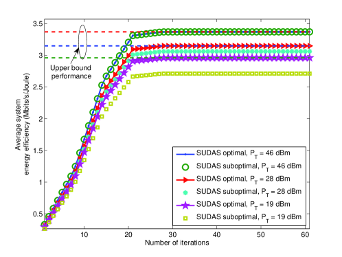
Figure 3: Average energy efficiency (Mbits/Joule) versus the number of iterations for different maximum transmit power budgets at the BS.

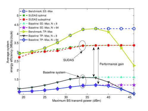
Figure 4: Average energy efficiency (Mbits/Joule) versus the maximum transmit power at the BS (dBm) for different communication systems. The double-sided arrows indicate the performance gain achieved by the proposed SUDAS.

V-B Average System Energy Efficiency versus Maximum Transmit Power

Figure 4 illustrates the average system energy efficiency versus the maximum DL transmit power at the BS for $M=8$ SUDACs for different systems and $N=8$ BS antennas. It can be observed that the average system energy efficiency of the two proposed resource allocation algorithms for SUDAS is a monotonically non-decreasing function of $P_{\mathrm{T}}$. In particular, starting from a small value of $P_{\mathrm{T}}$, the energy efficiency increases slowly with increasing $P_{\mathrm{T}}$ and then saturates when $P_{\mathrm{T}}>37$ dBm. This is due to the fact that the two proposed algorithms strike a balance between system energy efficiency and power consumption. In fact, once the maximum energy efficiency of the SUDAS is achieved, even if there is more power available for transmission, the BS will not consume extra DL transmit power for improving the data rate, cf. (38). This is because a further increase in the BS transmit power would only result in a degradation of the energy efficiency. Moreover, we compare the energy efficiency of the proposed SUDAS with a benchmark MIMO system and a baseline system. We focus on two system design objectives for the reference systems, namely, system throughput maximization (TP-Max) and energy efficiency maximization (EE-Max). For the benchmark MIMO system, we assume that each UE is equipped with $N$ receive antennas but the SUDAS is not used and optimal resource allocation is performed. Besides, we assume that the circuit power consumption at the UE does not scale with the number of antennas and only the licensed band is used for the benchmark system. In other words, the average system energy efficiency of the benchmark system serves as a performance upper bound for the proposed SUDAS. For the baseline system, we assume that the BS and the single-antenna UEs perform optimal resource allocation and utilize only the licensed frequency band, i.e., the SUDAS is not used. As can be observed from Figure 4, for high BS transmit power budgets, the SUDAS achieves more than $80\%$ of the benchmark MIMO system performance even though the UEs are only equipped with single antennas. Also, the SUDAS provides a huge system performance gain compared to the baseline system which does not employ SUDAS since the proposed SUDAS allows the single-antenna UEs to exploit spatial and frequency multiplexing gains. On the other hand, increasing the number of BS antennas dramatically in the baseline system from $N=8$ to $N=64$, i.e., to a large-scale antenna system, does not necessarily improve the system energy efficiency. In fact, in the baseline system, the higher power consumption, which increases linearly with the number of BS antennas, outweighs the system throughput gain, which only scales logarithmically with the additional BS antennas.

Figure 6 depicts the average time allocation for DL and UL transmission. It can be observed that the optimal time allocation depends on the transmit power budget of the systems. In particular, when the power budget of the BS for DL communication is small compared to the total transmit power budget for UL communication, e.g. $P_{\mathrm{T}}\leq 28$ dBm, the period of time allocated for DL transmission is shorter than that allocated for UL transmission. Because of the limited power budget and the circuit power consumption, it is preferable for the BS to transmit a sufficiently large power over a short period of time rather than a small power over a longer time to maximize the system energy efficiency and to fulfill the data rate requirement of the DL delay sensitive UEs. On the contrary, when the power budget of the BS is large compared to that of the UEs, the system allocates more time resources to the DL compared to the UL, since the BS can now transmit a large enough power to compensate the circuit power consumption for a longer time span to maximize the system energy efficiency.

V-C Average System Throughput versus Maximum Transmit Power

Figure 5: Average DL and UL transmission durations versus the maximum transmit power at the BS (dBm).

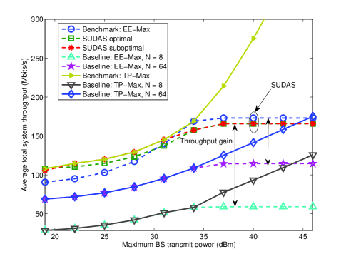
Figure 6: Average system throughput (Mbits/s) versus the maximum transmit power at the BS (dBm).

Figure 6 illustrates the average system throughput versus the maximum transmit power at the BS for $N=8$ BS antennas, $K=4$ UEs, and $M=8$. We compare the two proposed algorithms with the two aforementioned reference systems. The proposed SUDAS performs closely to the benchmark scheme in the low DL transmit power budget regime, e.g. $P_{\mathrm{T}}\leq 31$ dBm. This is due to the fact that the proposed SUDAS allows the single-antenna UEs to transmit or receive multiple parallel data streams by utilizing the large bandwidth available in the unlicensed band. Besides, for all considered systems, the average system throughput of all the systems increases monotonically with the maximum DL transmit power $P_{\mathrm{T}}$. Yet, for the systems aiming at maximizing energy efficiency, the corresponding system throughput saturates in the high transmit power allowance regime, i.e., $P_{\mathrm{T}}\geq 37$ dBm, in the considered system setting. In fact, the energy-efficient SUDAS does not further increase the DL transmit power since the system throughput gain due to a higher transmit power cannot compensate for the increased transmit power, i.e., the energy efficiency would decrease. As for the benchmark and baseline systems aiming at system throughput maximization, the average system throughput increases with the DL transmit power without saturation. For system throughput maximization, the BS always utilizes the entire available DL power budget. Yet, the increased system throughput comes at the expense of a severely degraded system energy efficiency, cf. Figure 4.

V-D Average System Performance versus Number of SUDACs

Figures 8 and 8 illustrate the average energy efficiency and throughput versus the number of SUDACs for $N=8$ BS antennas, $P_{\mathrm{T}}=37$ dBm, and different systems. It can be observed that both the system energy efficiency and the system throughput of the proposed SUDAS grows with the number of SUDACs, despite the increased power consumption associated with each additional SUDAC. For $N\geq M$, for DL transmission, additional SUDACs facilitate a more efficient conversion of the spatial multiplexing gain in the licensed band to a frequency multiplexing gain in the unlicensed band which leads to a significant data rate improvement. Similarly, for UL transmission, the SUDACs help in converting the frequency multiplexing gain in the unlicensed band to a spatial multiplexing gain in the licensed band. For $M>N$, increasing the number of SUDACs in the system leads to more spatial diversity which also improves energy efficiency and system throughput. Besides, a substantial performance gain can be achieved by the SUDAS compared to the baseline system for an increasing number of available SUDACs.

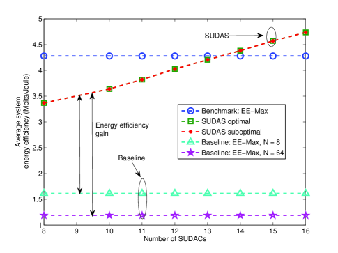
Figure 7: Average energy efficiency (Mbits/Joule) versus the number of SUDACs.

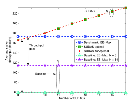
Figure 8: Average system throughput (Mbits/s) versus the number of SUDACs.

VI Conclusions

In this paper, we studied the resource allocation algorithm design for SUDAS assisted outdoor-to-indoor communication. Specifically, the proposed SUDAS simultaneously utilizes licensed and unlicensed frequency bands to facilitate spatial and frequency multiplexing gains for single-antenna UEs in DL and UL, respectively. The resource allocation algorithm design was formulated as a non-convex matrix optimization problem. In order to obtain a tractable solution, we revealed the structure of the optimal precoding matrices such that the problem could be transformed into a scalar optimization problem. Based on this result, we proposed an asymptotically globally optimal and a suboptimal iterative resource allocation algorithm to solve the problem by alternating optimization. Our simulation results showed that the proposed SUDAS assisted transmission provides substantial energy efficiency and throughput gains compared to baseline systems which utilize only the licensed frequency spectrum for communication.

Appendix-Proof of Theorem 2

Due to the page limitation, we provide only a sketch of the proof which follows a similar approach as in [25, 37] and uses majorization theory. We show that the optimal precoding and post-processing matrices jointly diagonalize the DL and UL end-to-end channel matrices on each subcarrier for the maximization of the transformed objective function in subtractive form in (IV-B). First, we consider the objective function in subtractive form for UE $k$ on a per-subcarrier basis with respect to the optimization variables. In particular, the per-subcarrier objective function for UE $k$ consists of two parts,

$$f_{1}({\cal P},{\cal S}) = -s^{[i,k]}_{\mathrm{DL}}\log_{2}\Big{(}\det[\mathbf{E}^{[i,k]}_{\mathrm{DL}}]\Big{)}-s^{[i,k]}_{\mathrm{UL}}\log_{2}\Big{(}\det[\mathbf{E}^{[i,k]}_{\mathrm{UL}}]\Big{)}$$ (56)

$$f_{2}({\cal P},{\cal S}) = s^{[i,k]}_{\mathrm{DL}}\varepsilon_{\mathrm{B}}\operatorname{\mathrm{Tr}}\Big{(}\mathbf{P}^{[i,k]}_{\mathrm{DL}}(\mathbf{P}^{[i,k]}_{\mathrm{DL}})^{H}\Big{)}+s^{[i,k]}_{\mathrm{DL}}\varepsilon_{\mathrm{S}}\operatorname{\mathrm{Tr}}\Big{(}\mathbf{G}^{[i,k]}_{\mathrm{DL}}\Big{)}+s^{[i,k]}_{\mathrm{UL}}\varepsilon_{\mathrm{S}}\operatorname{\mathrm{Tr}}\Big{(}\mathbf{G}^{[i,k]}_{\mathrm{UL}}\Big{)}$$ (57)

$$+ \varepsilon_{k}s^{[i,k]}_{\mathrm{UL}}\operatorname{\mathrm{Tr}}\Big{(}\mathbf{P}^{[i,k]}_{\mathrm{UL}}(\mathbf{P}^{[i,k]}_{\mathrm{UL}})^{H}\Big{)},$$

such that the maximization of the per subcarrier objective function can be expressed as

$$\underset{{\cal P},{\cal S}}{\operatorname{minimize}}-f_{1}({\cal P},{\cal S})+\eta_{\mathrm{eff}}f_{2}({\cal P},{\cal S}).$$ (58)

Besides, the determinant of the MSE matrix on subcarrier $i$ for UE $k$ can be written as

$$\det\Big{(}\mathbf{E}^{[i,k]}_{\mathrm{DL}}\Big{)} = \prod_{j=1}^{N_{\mathrm{S}}}\Big{[}\mathbf{E}^{[i,k]}_{\mathrm{DL}}\Big{]}_{j,j},$$ (59)

where $[\mathbf{X}]_{a,b}$ extracts the $(a,b)$-th element of matrix $\mathbf{X}$. $f_{1}({\cal P},{\cal S})$ is a Schur-concave function with respect to the optimal precoding matrices [25] for a given subcarrier allocation policy $\cal S$. Thus, $-f_{1}({\cal P},{\cal S})$ is minimized when the MSE matrix $\mathbf{E}^{[i,k]}_{\mathrm{DL}}$ is a diagonal matrix. Furthermore, the trace operator in $f_{2}({\cal P},{\cal S})$ for the computation of the total power consumption is also a Schur-concave function with respect to the optimal precoding matrices. Thus, the optimal precoding matrices for the minimization of function $f_{2}({\cal P},{\cal S})$ should diagonalize the input matrix of the trace function, cf. [38, Chapter 9.B.1] and [38, Chapter 9.H.1.h]. Similarly, the power consumption functions on the left hand side of constraints C1–C4 in (IV-B) are also Schur-concave functions and are minimized if the input matrices of the trace functions are diagonal. Besides, the non-negative weighted sum of Schur-concave functions over the subcarrier and UE indices preserves Schur-concavity. In other words, the optimal precoding matrices should jointly diagonalize the subtractive form objective function in (IV-B) and simultaneously diagonalize matrices $\mathbf{P}^{[i,k]}_{\mathrm{UL}}(\mathbf{P}^{[i,k]}_{\mathrm{UL}})^{H},\mathbf{P}^{[i,k]}_{\mathrm{DL}}(\mathbf{P}^{[i,k]}_{\mathrm{DL}})^{H},\mathbf{G}^{[i,k]}_{\mathrm{UL}}$, and $\mathbf{G}^{[i,k]}_{\mathrm{DL}}$. This observation establishes a necessary condition for the structure of the optimal precoding matrices. Finally, by performing SVD on the channel matrices and after some mathematical manipulations, it can be verified that the matrices in (27) and (28) satisfy the optimality condition.

References

• [1] M. Breiling, D. W. K. Ng, C. Rohde, F. Burkhardt, and R. Schober, “Resource Allocation for Outdoor-to-Indoor Multicarrier Transmission with Shared UE-side Distributed Antenna Systems,” in Proc. IEEE Veh. Techn. Conf., May 2015.
• [2] E. Larsson, O. Edfors, F. Tufvesson, and T. Marzetta, “Massive MIMO for Next Generation Wireless Systems,” IEEE Commun. Mag., vol. 52, pp. 186–195, Feb. 2014.
• [3] D. Ng, E. Lo, and R. Schober, “Energy-Efficient Resource Allocation in OFDMA Systems with Large Numbers of Base Station Antennas,” IEEE Trans. Wireless Commun., vol. 11, pp. 3292–3304, Sep. 2012.
• [4] K. Zheng, L. Zhao, J. Mei, M. Dohler, W. Xiang, and Y. Peng, “10 Gb/s HetSNets with Millimeter-Wave Communications: Access and Networking - Challenges and Protocols,” IEEE Commun. Mag., vol. 53, pp. 222–231, Jan. 2015.
• [5] H. Mehrpouyan, M. Matthaiou, R. Wang, G. Karagiannidis, and Y. Hua, “Hybrid Millimeter-Wave Systems: A Novel Paradigm for Hetnets,” IEEE Commun. Mag., vol. 53, pp. 216–221, Jan. 2015.
• [6] (2013) Ericsson Mobility Report. [Online]. Available: http://ec.europa.eu/digital-agenda/en/news/2014-report-implementation-eu-regulatory-framework-electronic-communications
• [7] (2013) Cost Model - Country Analysis Report (CAR) for Germany. [Online]. Available: http://www.ftthcouncil.eu/documents/Reports/2013/Cost_Model_CAR_Germany_August2013.pdf
• [8] A. Swindlehurst, E. Ayanoglu, P. Heydari, and F. Capolino, “Millimeter-Wave Massive MIMO: The Next Wireless Revolution?” IEEE Commun. Mag., vol. 52, pp. 56–62, Sep. 2014.
• [9] F. Boccardi, R. Heath, A. Lozano, T. Marzetta, and P. Popovski, “Five Disruptive Technology Directions for 5G,” IEEE Commun. Mag., vol. 52, pp. 74–80, Feb. 2014.
• [10] R. Heath, S. Peters, Y. Wang, and J. Zhang, “A Current Perspective on Distributed Antenna Systems for the Downlink of Cellular Systems,” IEEE Commun. Mag., vol. 51, pp. 161–167, Apr. 2013.
• [11] H. Zhu, “On Frequency Reuse in Cooperative Distributed Antenna Systems,” IEEE Commun. Mag., no. 4, pp. 85–89, Apr. 2012.
• [12] R. W. Heath, “What is the Role of MIMO in Future Cellular Networks: Massive? Coordinated? mmWave?” Presentation delivered at Int. Conf. on Commun., Jun. 2013. [Online]. Available: http://users.ece.utexas.edu/~rheath/presentations/2013/Future_of_MIMO_Plenary_Heath.pdf
• [13] M. Dohler, “Virtual Antenna Arrays,” Ph.D. dissertation, King’s College London, University of London, Nov. 2003.
• [14] T. Maciel and A. Klein, “On the Performance, Complexity, and Fairness of Suboptimal Resource Allocation for Multiuser MIMO–OFDMA Systems,” IEEE Trans. Veh. Technol., vol. 59, pp. 406–419, Jan. 2010.
• [15] C.-M. Yen, C.-J. Chang, and L.-C. Wang, “A Utility-Based TMCR Scheduling Scheme for Downlink Multiuser MIMO-OFDMA Systems,” IEEE Trans. Veh. Technol., vol. 59, pp. 4105–4115, Oct. 2010.
• [16] H. Zhu and J. Wang, “Resource Allocation in OFDMA-Based Distributed Antenna Systems,” in Proc. IEEE/CIC IEEE Intern. Commun. Conf. in China, Aug 2013, pp. 565–570.
• [17] CISCO: The Internet of Things. [Online]. Available: http://share.cisco.com/internet-of-things.html
• [18] J. Jiang, M. Dianati, M. Imran, and Y. Chen, “Energy Efficiency and Optimal Power Allocation in Virtual-MIMO Systems,” in Proc. IEEE Veh. Techn. Conf., Sep. 2012.
• [19] C. He, B. Sheng, P. Zhu, X. You, and G. Li, “Energy- and Spectral-Efficiency Tradeoff for Distributed Antenna Systems with Proportional Fairness,” IEEE J. Select. Areas Commun., vol. 31, pp. 894–902, May 2013.
• [20] X. Chen, X. Xu, and X. Tao, “Energy Efficient Power Allocation in Generalized Distributed Antenna System,” IEEE Commun. Lett., vol. 16, pp. 1022–1025, Jul. 2012.
• [21] SUDAS - UE-Side Virtual MIMO using MM-Wave for 5G. [Online]. Available: www.iis.fraunhofer.de/sudas
• [22] J. Andrews, “Seven Ways that HetNets are a Cellular Paradigm Shift,” IEEE Commun. Mag., vol. 51, pp. 136–144, Mar. 2013.
• [23] D. W. K. Ng and R. Schober, “Cross-Layer Scheduling for OFDMA Amplify-and-Forward Relay Networks,” IEEE Trans. Veh. Technol., vol. 59, pp. 1443–1458, Mar. 2010.
• [24] I. Hammerstrom and A. Wittneben, “Power Allocation Schemes for Amplify-and-Forward MIMO-OFDM Relay Links,” IEEE Trans. Wireless Commun., vol. 6, pp. 2798–2802, Aug. 2007.
• [25] Y. Rong, X. Tang, and Y. Hua, “A Unified Framework for Optimizing Linear Nonregenerative Multicarrier MIMO Relay Communication Systems,” IEEE Trans. Signal Process., vol. 57, pp. 4837 – 4851, Dec. 2009.
• [26] D. W. K. Ng, E. S. Lo, and R. Schober, “Energy-Efficient Resource Allocation in Multi-Cell OFDMA Systems with Limited Backhaul Capacity,” IEEE Trans. Wireless Commun., vol. 11, pp. 3618–3631, Oct. 2012.
• [27] W. Dinkelbach, “On Nonlinear Fractional Programming,” Management Science, vol. 13, pp. 492–498, Mar. 1967.
• [28] W. Yu and R. Lui, “Dual Methods for Nonconvex Spectrum Optimization of Multicarrier Systems,” IEEE Trans. Commun., vol. 54, pp. 1310 – 1321, Jul. 2006.
• [29] K. Seong, M. Mohseni, and J. Cioffi, “Optimal Resource Allocation for OFDMA Downlink Systems,” in Proc. IEEE Intern. Sympos. on Inf. Theory, Jul. 2006, pp. 1394–1398.
• [30] J. C. Bezdek and R. J. Hathaway, “Convergence of Alternating Optimization,” Neural, Parallel and Sci. Comput., vol. 11, pp. 351 –368, Dec. 2003.
• [31] J. Meinilä, P. Kyösti, L. Hentilä, T. Jämsä, E. K. Essi Suikkanen, and M. Narandžić, “Wireless World Initiative New Radio WINNER+, D5.3: WINNER+ Final Channel Models,” CELTIC Telecommunication Soultions, Tech. Rep.
• [32] “Technical Specification Group Radio Access Network; Evolved Universal Terrestrial Radio Access (E-UTRA); Physical Channels and Modulation (Release 8),” 3rd Generation Partnership Project, Tech. Rep., 3GPP, TS 36.211, V8.9.0.
• [33] A. Maltsev, V. Erceg, E. Perahia, C. Hansen, R. Maslennikov, A. Lomayev, A. Sevastyanov, A. Khoryaev, G. Morozov, M. Jacob, T. K. S. Priebe, S. Kato, H. Sawada, K. Sato, and H. Harada, “Channel Models for 60 GHz WLAN Systems,” IEEE Tech. Rep. 802.11-09/0334r8, Tech. Rep.
• [34] O. Arnold, F. Richter, G. Fettweis, and O. Blume, “Power Consumption Modeling of Different Base Station Types in Heterogeneous Cellular Networks,” in Proc. Future Network and Mobile Summit, 2010, pp. 1–8.
• [35] R. Kumar and J. Gurugubelli, “How Green the LTE Technology Can be?” in Intern. Conf. on Wireless Commun., Veh. Techn., Inform. Theory and Aerosp. Electron. Syst. Techn., Mar. 2011.
• [36] M. Miyahara, H. Sakaguchi, N. Shimasaki, and A. Matsuzawa, “An 84 mW 0.36 $\mbox{mm}^{2}$ Analog Baseband Circuits For 60 GHz Wireless Transceiver in 40 nm CMOS,” in Proc. IEEE Radio Freq. Integr. Circuits Sympos. (RFIC), Jun. 2012, pp. 495–498.
• [37] D. W. K. Ng, E. S. Lo, and R. Schober, “Dynamic Resource Allocation in MIMO-OFDMA Systems with Full-Duplex and Hybrid Relaying,” IEEE Trans. Commun., vol. 60, pp. 1291–1304, May 2012.
• [38] A. W. Marshall and I. Olkin, Inequalities: Theory of Majorization and its Applications.   New York: Academic Press, 1979.