Does communication enhance pedestrians transport in the dark?

Abstract

We study the motion of pedestrians through an obscure tunnel where the lack of visibility hides the exits. Using a lattice model, we explore the effects of communication on the effective transport properties of the crowd of pedestrians. More precisely, we study the effect of two thresholds on the structure of the effective nonlinear diffusion coefficient. One threshold models pedestrians’s communication efficiency in the dark, while the other one describes the tunnel capacity. Essentially, we note that if the evacuees show a maximum trust (leading to a fast communication), they tend to quickly find the exit and hence the collective action tends to prevent the occurrence of disasters.

Résumé Nous étudions la dynamique des movements de foules dans un tunnel dont la visibilité est très reduite. Tout en particulier, nous nous intéréssons á des tunnels dont les sorties ne sont pas visibles. Á l’aide de notre modèle – un automate cellullaire – nous éxploitons les éffets de la communication inter–personnelle parmis les piétons sur la structure de la nonlinearité du coefficient de diffusion. Nous modélisons l’éfficacité de la communication inter–personnelle ainsi que la capacité des sorties á l’aide de deux barrières.

, ,

1 Introduction

This Note deals with the following evacuation scenario: A possibly large group of pedestrians needs to evacuate a long and obscure tunnel. The lack of visibility is due to either an electricity breakdown or due to a dense smoke. The basic modeling assumption is that the pedestrians are equally fit, do not know each other, and also, are unaware of the precise geometry of the tunnel. We wish to build a lattice model to explore the effects of communication on the effective transport properties of these pedestrians. As modeling tool, we use a particular type of particle system, known as zero range process (abbreviated here ZRP), whose dynamics is affected by two thresholds. One threshold - called activation threshold – models pedestrians’s communication efficiency in the dark, while the other one – the saturation threshold – describes the tunnel capacity. From the modeling point of view, the activation threshold is open to many interpretations. In this Note, we associate the size of this threshold not only with the geometric level of the possibility of communication, but also with the willingness and ability of the pedestrians to process the transmitted information to make a decision towards orientation to a potential exit or choice of speed in the dark. We refer to this as level of trust. Essentially, a small activation threshold implies in this context a high level of trust.

In Fig. 1 we sketch the meaning of the two thresholds, the precise mathematical definition is given in Section 2. Each solid circle represents a pedestrian, whereas the associated open (bigger) circle represents its communication domain and level of trust. On left bottom, the number of pedestrians in the cell is so small that their typical distance is larger than the radius of the communication domain. On left top we see that if the number of pedestrian is large enough information can propagate throughout the cell. In other words, we assume that the information can be efficiently transmitted among the different pedestrians as soon as any single communication domain (the open circles) intersects at least one other pedestrian. Essentially, we need here a minimal degree of packing of the open circles, which is guaranteed in our scenario by the activation threshold.

On the right bottom part we indicate that provided the number of pedestrians in the cell is smaller than the number that can be accommodated at boundaries, then it increases proportionally to the number of pedestrians in the cell. If the number of pedestrians in the cell is too high (see right top), than the number of them exiting the cell per unit time saturates.

It is worth mentioning that thresholds–biased dynamics have been discussed also for other transportation scenarios; compare e.g. [1, 2, 3] (group formation and cooperation in the dark) and [4, 5] (collective dynamics of molecular motors). This Note focusses on communication efficiency and is organized as follows: our transport model is described in Section 2, while Section 3 contains the hydrodynamic limit of the model as well as numerical illustrations exploring the effects of communication on the effective transport properties of the crowd of pedestrians traveling the obscure tunnel.

Figure 1: Sketch of pedestrians moving through a cell of the obscure tunnel driven by a two-threshold biased dynamics.

2 The model

We consider a positive integer $L$ and define a zero range process (ZRP) [6, 7] on the finite torus (periodic boundary conditions) $\Lambda:=\{1,\dots,L\}\subset{\mathbb{Z}}$. Fix $N\in{\mathbb{Z}}_{+}$ and consider the finite state or configuration space $\Omega:=\{0,\dots,N\}^{\Lambda}$. Given $\omega=(\omega_{1},\dots,\omega_{L})\in\Omega$ the integer $\omega_{x}$ is called number of particle at site $x\in\Lambda$ in the state or configuration $\omega$. We pick $A,S\in\{1,\dots,N\}$ with $S\geq A$, the activation and saturation thresholds, respectively. We define the intensity function

$$g(k)=\left\{\begin{array}[]{ll}0&\textrm{ if }k=0\\ 1&\textrm{ if }1\leq k\leq A\\ k-A+1&\textrm{ if }A<k\leq S\\ S-A+1&\textrm{ if }k>S\\ \end{array}\right.$$ (1)

for each $k\in{\mathbb{Z}}_{+}$. The ZRP we consider here is the Markov process $\omega_{t}\in\Omega$, with $t\geq 0$, such that each site $x\in\Lambda$ is updated with intensity $g(\omega_{x}(t))$ and, once such a site $x$ is chosen, a particle jumps with probability $1/2$ to the neighboring right site $x+1$ or with probability $1/2$ to the neighboring left site $x-1$. For more details on this modeling strategy, see [6].

The intensity function relates to the hopping rates $r^{(x,x\pm 1)}(\omega_{x}(t))=g(\omega_{x}(t))/2$ and coincides with the escape rate $r^{(x,x-1)}(\omega_{x}(t))+r^{(x,x+1)}(\omega_{x}(t))=g(\omega_{x}(t))$ at which a particle leaves the site $x$. The thresholds intend to control the escape rate. Essentially, the activation threshold $A$ keeps the escape rate low for all sites for which $\omega_{x}(t)\leq A$, regardless the number of particles on $x$. The saturation threshold $S$ holds the escape rate fixed to a maximum value for all sites for which $\omega_{x}(t)\geq S$, regardless, again, the number of particles on $x$. In the intermediate case, $A<\omega_{x}(t)<S$ the escape rate increases proportionally to the actual number of particles on $x$, see (1). In the limiting case $A=1$ and $S=\infty$, the intensity function becomes $g(k)=k$, for $k>0$, and thus the well-known independent particle model is recovered. A different limiting situation appears when the intensity function is $1$ for any $k\geq 1$ and $0$ for $k=0$. For this we find a ZRP whose configurations can be mapped to a simple exclusion–like model states (cf. e.g. [7]). Interestingly, we can tune between the two very different dynamics either by keeping $S=\infty$ and varying $A$ or by keeping $A=1$ and varying $S$.

3 Hydrodynamic limit. Threshold effects

We study the hydrodynamic limit $N,L\to\infty$. Particularly, we exploit the fact that the intensity function is not decreasing and use well–established theories to derive the limiting non–linear diffusion coefficient and the limiting current in presence of the two thresholds. The Gibbs measure with fugacity $z\in\mathbb{R}_{+}$ of the ZRP introduced above is the product measure $\nu_{z}(\eta_{1})\nu_{z}(\eta_{2})\cdots\nu_{z}(\eta_{L})$ on $\mathbb{N}^{\Lambda}$ for any $\eta=(\eta_{1},\dots,\eta_{L})\in\mathbb{N}^{\Lambda}$ with $\nu_{z}(0)=C_{z}$ and $\nu_{z}(k)=C_{z}z^{k}/[g(1)\cdots g(k)]$ for $k\geq 1$, where $C_{z}$ is a normalization factor depending on $z$, $A$, and $S$, namely, $1/C_{z}=1+\sum_{k=1}^{\infty}z^{k}/[g(1)\cdots g(k)].$ To compute the mean value of the intensity function $g$, we use $\nu_{z}(0)$ with $g(0)=0$ to get

$$\nu_{z}[g(\omega_{x})]=\sum_{k=1}^{\infty}\nu_{z}(k)\,g(k)=C_{z}z+C_{z}z\sum_{k=2}^{\infty}\frac{z^{k-1}}{g(1)\cdots g(k-1)}=z\,\,.$$ (2)

As a function of the activity, the expectation does not depend on the particular choice of the intensity function.

For what concerns the hydrodynamic limit, a special role will be played by the density

$$\bar{\rho}(z)=\sum_{k=0}^{\infty}k\,\nu_{z}(k)\,.$$ (3)

Note that $\bar{\rho}(z)$ is an increasing function of the fugacity, indeed, $\partial\bar{\rho}(z)/\partial z=[\nu_{z}(\eta_{1}^{2})-(\nu_{z}(\eta_{1}))^{2}]/z>0$. Hence, it is possible to define $\bar{z}(\rho)$ as the inverse function of $\bar{\rho}(z)$. We observe that $\bar{\rho}$ is defined for any positive $z$ if $A$ is finite and $S=\infty$.

The evolution of the distribution of the particles on the space $\Lambda$ under the ZRP with thresholds $A$ and $S$ can be described in the diffusive hydrodynamic limit via the time evolution of the density function $\rho(x,t)$ with the space variable $x$ varying in the interval $[0,1]$ and for any time $t\geq 0$; compare [6]. Consequently, the continuous space density $\rho(x,t)$ is the solution of the partial differential equation

$$\frac{\partial}{\partial t}\rho=-\frac{\partial}{\partial x}{J(\varrho)}\;\;\textrm{ with }\;\;J(\varrho)=-\frac{1}{2}D(\rho)\frac{\partial}{\partial x}\rho$$ (4)

where the macroscopic flux $J(\varrho)$ incorporates the effective diffusion coefficient $D$ given by

$$D(\rho)=\frac{\partial}{\partial\rho}\nu_{\bar{z}(\rho)}\left[g(\omega_{1})\right]\,.$$ (5)

The coefficient $D$ is computed in terms of the mean of the intensity function evaluated against the single site Gibbs measure with fugacity corresponding to the local value of the density. Consequently, $D$ depends of the value of the thresholds.

Let us discuss the effects induced by the two thresholds $A$ and $S$ on the diffusion coefficient. We first recall some known results which are valid in the two limiting situations $A=1$ and $S=\infty$ (independent particle model) and $A=S$ (simple exclusion–like model). In the first case, one has $C_{z}=\exp\{-z\}$. Hence, by (3), it holds $\bar{\rho}(z)=z$. Recalling (2) and the definition of $\bar{z}$, we have $\nu_{\bar{z}(\rho)}\left[g(\omega_{1})\right]=\nu_{\rho}\left[g(\omega_{1})\right]=\rho$. By using (5), the diffusion coefficient reads $D(\rho)=1$. On the other hand, in the latter case, one has $g(k)=1$ for any $k\geq 1$ and $g(0)=0$. Hence, $C_{z}=1-z$, and it holds $\bar{\rho}(z)=z/(1-z)$. Here, one finds the law $D(\rho)=1/(1+\rho)^{2}$, cf. [8]. Now, we illustrate the general strategy to compute the diffusion coefficient $D$ for arbitrary values of the thresholds $A$ and $S$. To do so, we first compute $\bar{\rho}(z)$. The precise expression of the diffusion coefficient can be then obtained using the general recipe in equation (5) and recalling (2). Indeed,

$$D(\rho)=\frac{\partial}{\partial\rho}\nu_{\bar{z}(\rho)}\left[g(\omega_{1})\right]=\frac{\partial}{\partial\rho}\bar{z}(\rho)=\Big{(}\frac{\partial}{\partial z}\bar{\rho}(z)\Big{)}^{-1}\Big{|}_{z=\bar{z}(\rho)}$$ (6)

The explicit expression of $\partial\bar{\rho}(z)/\partial z$ appearing in (6) is lengthy, hence we omit it.

Fig. 2 shows the behavior of the diffusion coefficient as a function of the local density, and parametrized by the values of the thresholds. The upper left panel refers to the case $A=1$ and for different values of $S$: the simple exclusion–like model is recovered for $S=1$, while the independent particle model appears for $S=\infty$. Similarly, the upper right panel illustrates the case with $S=\infty$ and for different values of $A$: here the independent particle model corresponds to $A=1$ and the simple exclusion–like model is recovered for $A=\infty$. In both the upper panels of the figure we see that for the independent particle case, the diffusion coefficient is constant with respect to the local density.

Furthermore, in Fig. 2, we remark the loss of monotonicity of the function $D(\rho)$ for values of $\rho$ exceeding some critical value (depending on the thresholds $A$ and $S$). The behavior of $D(\rho)$ displayed in the lower left panel refers to the case $A=3$. Considering particularly the green curve corresponding to $S=10$, one sees the onset of a double loss of monotonicity of the function $D(\rho)$: for small values of the density, $D$ stays close to the simple exclusion–like behavior and decreases with $\rho$. After one first critical value of the density, it starts rising up, until it drops down again, when $\rho$ exceeds an upper critical value. This indicates the presence of a double threshold for the intensity function given by (1).

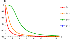
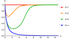
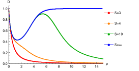
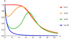
Figure 2: Left panel, top row: Diffusion coefficient $D(\rho)$ vs. $\rho$ for $A=1$ and for different values of the saturation threshold, i.e., $S=1,2,5,\infty$. Right panel, top row: Diffusion coefficient $D(\rho)$ vs. $\rho$ for $S=\infty$ and for different values of the activation threshold, i.e., $A=1,2,5,\infty$. Left panel, bottom row: Diffusion coefficient $D(\rho)$ vs. $\rho$ for $A=3$ and for $S=3,4,10,\infty$. Right panel, bottom row: Diffusion coefficient $D(\rho)$ vs. $\rho$ for $S=10$ and for $A=1,2,5,10$.

In the lower right panel of Fig. 2, the diffusion coefficient is plotted for different values of $A$ for the case $S=10$. The red and the blue curves refer to the extreme independent–particle and simple–exclusion–like cases. When the activation threshold is varied two effects are prominent: the non–monotonicity of the diffusion coefficient with respect to density shows up and, at fixed local density, the diffusion coefficient decreases when $A$ is increased. Interestingly, note that for local densities close to $8$ this appears not to be true: increasing the activation threshold induces an increase in the diffusion coefficient. For this very particular regime the dynamics accelerates due to the increase in the activation threshold. In other words, it seems that close to the local density $8$ (which, depending on the population type, is close to the maximum pedestrians density before asphyxiation starts off), higher mistrust speeds up the dynamics.

Excepting the just mentioned non–intuitive regime, the effect of the two thresholds on the diffusion coefficient can be summarized as follows: the smaller the activation threshold $A$ and/or the higher the saturation threshold $S$, the higher is the diffusion coefficient, and therefore, the quicker the dynamics. From the evacuation viewpoint, “a small activation threshold increases the diffusion coefficient” means that

higher trust among pedestrians improves communication in the dark

and therefore the exits can be found easier. The size of the saturation threshold simply decides on the exit capacity. Consequently, a higher saturation threshold leads to an improved capacity of the exists (e.g. larger doors, or more exits [9]) and therefore the evacuation rate is correspondingly higher.

Acknowledgements.

We thank E. Presutti (GSSI L’Aquila, Italy), A. De Masi (L’Aquila, Italy), and C. Landim (IMPA, Brazil) for useful discussions. ENMC thanks ICMS (TU/e, Eindhoven, The Netherlands) for the very kind hospitality and for financial support.

References

- [1] Cirillo, E.N.M., Muntean, A.: Can cooperation slow down emergency evacuations?. Comptes Rendus Mecanique 340, 626–628 (2012).
- [2] Muntean, A., Cirillo, E.N.M., Krehel, O., Böhm, M. Pedestrians moving in the dark : balancing measures and playing games on lattices. In A. Muntean F. Toschi (Eds.), Collective dynamics from bacteria to crowds : an excursion through modeling, analysis and simulation (pp. 75-103). Vienna: Springer.
- [3] Cirillo, E.N.M., Muntean, A.: Dynamics of pedestrians in regions with no visibility : a lattice model without exclusion. Physica A: Statistical Mechanics and Its Applications, 392(17), 3578–3588 (2013).
- [4] Leibler, S, Huse, D. A.: Porters versus rowers: a unified stochastic model of motor proteins. J. Cell Biol. 121(6), 1357D1368 (1993).
- [5] Campàs, O., Kafri, Y., Zeldovich, K. B., Casademunt, J., Joanny, J.-F.: Collective dynamics of interacting motors. Phys. Rev. Lett. 97, 038101 (2006).
- [6] De Masi, A., Presutti, E.: Mathematical Methods for Hydrodynamic Limits, Springer–Verlag, Berlin Heidelberg (1991).
- [7] Evans, M. R., Hanney, T.: Nonequilibrium statistical mechanics of the zero–range process and related models. J. Phys. A: Math. Gen. 38, R195–R240 (2005).
- [8] Ferrari, P. A., Presutti, E., Vares, M.E.: Local equilibrium for a one dimensional zero range process. Stoch. Proc. Appl. 26, 31–45 (1987).
- [9] K. Fridolf, E. Ronchi, D. Nilsson, H. Frantzich, Movement speed and exit choice in smoke-filled rail tunnels. Fire Safety Journal 59, 8-21, (2013).