A mechanical model for guided motion of mammalian cells

Abstract

We introduce a generic, purely mechanical model for environment-sensitive motion of mammalian cells that is applicable to chemotaxis, haptotaxis, and durotaxis as modes of motility. It is able to theoretically explain all relevant experimental observations, in particular, the high efficiency of motion, the behavior on inhomogeneous substrates, and the fixation of the lagging pole during motion. Furthermore, our model predicts that efficiency of motion in following a gradient depends on cell geometry (with more elongated cells being more efficient).

Motility and directed cell motion play an important role in many biological processes ranging from embryonic development Chicurel (2002); Gray et al. (2003); Huttenlocher and Horwitz (2011) to tissue invasion by pathogenic microorganisms Chicurel (2002); Gray et al. (2003); Prost et al. (2008); Parsons et al. (2010) and cancer progression Lo et al. (2000); Gerisch and Chaplain (2008); Bordeleau and Galarneau (2010); Parsons et al. (2010).

Often extracellular cues are used to regulate the decision in which direction the cell will move Macnab and Koshland (1972); Tindall et al. (2008a); Levine and Rappel (2008). Depending on these cues one distinguishes between: (1) chemotaxis where directed motion is guided by solvent chemical cues Macnab and Koshland (1972); (2) haptotaxis where substrate-bound cues influence the cell-substrate adhesiveness Carter (1965); and (3) durotaxis where mechanical cues such as substrate rigidity influence the directed motion Lo et al. (2000).

Physics-based experimental and theoretical approaches to study these phenomena have attracted considerable interest in the last decade. Many studies have been devoted to bacterial chemotaxis Tindall et al. (2008a, b); Adler (1966); Macnab and Koshland (1972); Adler (1975); Tu et al. (2008); Zhu et al. (2012) and to Dictiostelium discoideum as model system for amoeboid migration Fisher et al. (1989); Fuller et al. (2010); Hecht et al. (2011); Levine and Rappel (2008); Buenemann et al. (2010); Camley et al. (2013). The main challenge is to analyze and theoretically model the interplay between molecular processes and the emerging macroscopic motion. For amoeboid motion this is further complicated as shape changes have to be taken into account Buenemann et al. (2010); Hecht et al. (2011); Camley et al. (2013).

In contrast, the mesenchymal migration of mammalian cells has so far not been studied theoretically. Although many details have been characterized experimentally Zaman et al. (2005); Häcker (2012); Gerisch and Chaplain (2008) theoretical studies have focused only on the cell shape during migration Rubinstein et al. (2005), on continuum descriptions for cell populations Gerisch and Chaplain (2008); Häcker (2012) or on special short-term aspects of migration like migration speed DiMilla et al. (1991) or effective adhesiveness Zaman et al. (2005).

In this paper we study the motility of mammalian epithelial-like cells. They are influenced by a variety of chemical and physical signals, in particular by different mechanical forces Butcher et al. (2009) and can show a very high efficiency in following all kinds of gradients Theveneau et al. (2010). Mammalian cells predominantly migrate by a crawling motion Keren and Theriot (2008). It consists of a cycle of five discrete steps carried out within about ten minutes Mogilner (2009); Lauffenburger and Horwitz (1996); Pathak and Kumar (2011); Ridley et al. (2003); DiMilla et al. (1991); Zaman et al. (2005); Parsons et al. (2010); Huttenlocher and Horwitz (2011); Chicurel (2002); Keren and Theriot (2008): (1) polarization of the cell yielding a defined leading and a defined lagging pole; (2) formation of protrusions (predominantly) at the leading pole and attachment of the lagging pole, see Fig. 1(a); (3) stabilization of these protrusions by adhesion to the substrate or the extracellular matrix (ECM); (4) translocation of the cell-body by myosin-mediated contraction; (5) retraction of the rear by loosening the adhesions at the lagging pole. This crawling is propelled by the active lamellipodeum at the leading edge which pulls the passive cell body forward Friedl (2004). Cell motility depends on the stiffness of the substrate and the ECM. These effects are mediated indirectly via their impact on cell shape Holmes and Edelstein-Keshet (2012) and directly through so far unresolved mechanisms referred to as durotaxis Lo et al. (2000); Trichet et al. (2012); Provenzano et al. (2008); Yeung et al. (2005); Gray et al. (2003).

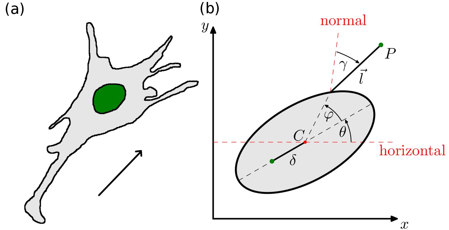
Figure 1: (a) Typical cell shape as observed in Lo et al. (2000) for a cell polarized in the direction of the arrow. The protrusions mainly grow into the forward direction. (b) In our model the polarized cell is represented by an ellipse, the attachments by lines. The position of an attachment point is defined by the length of a protrusion and three angles: the rotation angle of the cell $\theta$, the angle $\varphi$ for the attachment position on the cell membrane, and the angle $\gamma$ between the central line and the arm. The distance between the center of the ellipse and the anchor point is $\delta$.

The mechanical interaction with the substrate or the ECM can be thought of as a bilinear sequential binding Pathak and Kumar (2011), which affects the cell predominantly on the nanoscale through mechanosensing mechanisms Butcher et al. (2009); Trichet et al. (2012). However, cells can also chemically manipulate the ECM, e.g., in case of cancer, where tumor cells stiffen the surrounding ECM Butcher et al. (2009); Provenzano et al. (2008), and build a rigid stroma around the tumor. This step in ECM stiffness then promotes cells from the outside moving inside, but prevents cells from the inside to migrate outside Bordeleau et al. (2013). In general, mammalian cells are not passive recipients of mechanical forces, but actively respond by pulling or pushing the ECM Lauffenburger and Horwitz (1996); Lo et al. (2000); Butcher et al. (2009).

We introduce here a simple, generic model for environment-sensitive motion of fibroblast-like cells. It is solely based on mechanics and is applicable to chemotaxis, haptotaxis, and durotaxis as modes of motility. It provides the first theoretical explanation of the high efficiencies of mesenchymal-like motion independent of cellular morphology. Our model also covers the motility dynamics on large time scales. In particular, we can capture the statistical properties at environmental discontinuities, e.g., a step in substrate stiffness or a step in concentration of a chemo-attractant. These results indicate that regulation of taxis might be based on mechanical forces.

In our model we represent the polarized cell body by an ellipse with major radius $R_{l}$ and minor radius $R_{s}$. The orientation with respect to the $x$-axis is measured by the angle $\theta$ that parameterizes rotation around the center $C$. To counterbalance the forces of the protrusions the cell is attached to the surface at an anchor point. Moving cells typically have a shape similar to the one shown in fig. 1(a) with a single elongated tail that appears when the cell-body moves forward. This indicates that there is only a single anchor point. The motion occurs in such a way that the cell is effectively rotated around this anchor point, see Fig. 1(b). In principle, cells could also fix the position of the tail with several anchor points. Then, the cell is effectively rotated around these fixed points. For simplicity, we restrict here the analysis to a single anchor point. We assume that the anchor point remains at a fixed position while the cell is not moving. Real cells might change their shape during motion that could lead to a change in the position of the anchor point. However, we do not take such effects into account.

In the following we assume that a molecular mechanism initially polarizes the cell along the $x$-axis (for example in the presence of a gradient as discussed below). For our purpose we do not explicitly model this process and assume that it leads to a normally distributed initial angle $\theta\left(t=0\right)$ with mean $\mu_{\theta}=0$. The standard deviation $\sigma_{\theta}$ was estimated by fitting a normal distribution to the polarization model shown in Levine and Rappel (2013).

The protrusions by which the cells pull themselves forward are represented by adhesive arms that grow out of the ellipse at a random angle $\varphi$ with probability distributions given by Gaussian distributions centered around $\varphi=0$ (for the leading pole) and $\varphi=\pi$ (for the lagging pole)

$$p(\varphi)=\frac{p_{+}}{\sqrt{2\pi}\sigma_{+}}e^{-\varphi^{2}/2\sigma_{+}^{2}}+\frac{p_{-}}{\sqrt{2\pi}\sigma_{-}}e^{-(\varphi-\pi)^{2}/2\sigma_{-}^{2}}.$$ (1)

The weights $p_{+}$ of the leading pole and $p_{-}=1-p_{+}<p_{+}$ of the lagging pole reflect the initial polarization of the cell and shift the arm distribution towards the leading pole.

Length and direction of the arms are random. For simplicity, we draw the angle $\gamma$ between growth direction and surface normal from a Gaussian distribution with mean $\mu_{\gamma}=0$ and standard deviation $\sigma_{\gamma}$. Similarly, the arm length $l$ is distributed normally with mean $\mu_{l}$ and standard deviation $\sigma_{l}$.

Arm formation occurs at constant rate. Every arm applies a linear force on the cell that is proportional to the concentration of a chemoattractant or rigidity of the substrate. Thus, if at time $t$ there are $N$ arms that are attached to the cell body at position $\bm{x}_{i}=\bm{x}_{i}(\varphi_{i})$ pointing in direction $\bm{l}_{i}$ (with $1\leq i\leq N$) the total force on the cell is given by

$$\bm{F}\left(\bm{r}_{\mathrm{cell}},\theta,t\right)=\sum_{i=1}^{N}\bm{F}_{i}=\sum_{i=1}^{N}k\left(c\right)\bm{l}_{i}\left(\bm{r}_{\mathrm{cell}},\theta,\varphi_{i}\right),$$ (2)

where $k\left(c\right)=k_{0}c\left(\bm{r}_{\mathrm{arm}}\right)$ depends on the chemoattractant concentration or the substrate rigidity $c\left(\bm{r}\right)$. This results in a translocation of the cell. Furthermore, the arms exert a total torque $M\left(\bm{r}_{\mathrm{cell}},\theta,t\right)=\sum_{i=1}^{N}\left(\bm{x_{i}}\times\bm{F_{i}}\right)_{z}$, that leads to a rotation of the cell that can be interpreted as a gradual repolarization of the cell.

For most of our simulations we used a linear gradient of fixed strength $c_{0}={1}/{R_{l}}$. This results in a standard deviation of the initial angle of $\sigma_{\theta}\approx 1$.

To classify the planar cell motion (in the $x$-$y$ plane), we numerically calculated the moments $\left\langle x\right\rangle$, $\left\langle y\right\rangle$,$\left\langle x^{2}\right\rangle$, and $\left\langle y^{2}\right\rangle$, where $\langle...\rangle$ denotes the average over 500 independent runs, see Fig. 2. In these simulations we implemented the above mentioned cycle of independent steps (1)-(5). Starting from the polarized shape [step (1)] we grow $N$ new arms of lengths $l_{i}$ at angles $\varphi_{i}$ in every iteration [steps (2) and (3)]. The new position and orientation of the cell is then obtained by solving $\bm{F}\left(\bm{r}_{\mathrm{cell}},\theta,t\right)=0$ and $M\left(\bm{r}_{\mathrm{cell}},\theta,t\right)=0$ independently [step (4)]. Then, all arms are removed [step (5)], the time is increased by $\delta t$ and the iteration starts over. In the absence of a gradient the cells perform an isotropic random walk. For $N=10$ (for parameter values see Sup ) the effective diffusion coefficients $D_{x}\approx D_{y}=43.77{R_{l}^{2}}/{\delta t}$ were measured by fitting linear functions to $\langle x^{2}\rangle$ and $\langle y^{2}\rangle$.

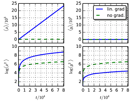
Figure 2: Classification of cell motion as obtained from the numerically calculated moments $\left\langle x\right\rangle$, $\left\langle y\right\rangle$,$\left\langle x^{2}\right\rangle$, and $\left\langle y^{2}\right\rangle$. In the absence of gradients the cell performs a random walk characterized by vanishing $\left\langle x\right\rangle$ and $\left\langle y\right\rangle$ and standard deviations that increase with time. In the presence of a gradient this random walk becomes biased. In this case the motion in $y$-direction is suppressed compared with the case of no gradient. Data were obtained by averaging over 500 independent runs. Length and time are given in units of $R_{l}$ and $\delta t$, respectively.

In this limit the model can also be solved analytically. From the one-dimensional probability densities of $\varphi$, $\gamma$ and $l$ the two-dimensional probability density of the force induced by an arm can be calculated Sup . We have compared these analytical results with those obtained by direct numerical integration of the model and found excellent agreement. It is interesting to note that this force probability density resembles the shapes of migrating lamellipodial domains of keratocytes Rubinstein et al. (2005). If one assumes that these shape deformations reflect the forces then the forces acting on the cell in our simple probabilistic model are remarkably similar to those exerted by the actin cytoskeleton of keratocytes.

Next, we consider substrates with gradients. For a linear gradient $c_{0}={1}/{R_{l}}$ parallel to the $x$-axis, the cells perform a biased random walk in the gradient direction while the motion in the perpendicular direction is suppressed $\sim 135$-fold ($D_{y}=0.32{R_{l}^{2}}/{\delta t}$ in presence of a gradient compared to $D_{y}=43.77{R_{l}^{2}}/{\delta_{t}}$ in absence of a gradient), see Fig. 2. To quantify the efficiency of the motion in following the applied gradient we measured the chemotactic factor

$$CF=\left\langle\frac{L_{\mathrm{grad}}}{L_{\mathrm{tot}}}\right\rangle.$$ (3)

Here, $L_{\mathrm{tot}}$ is the total path length and $L_{\mathrm{grad}}$ the length of the projection in the direction of the gradient.

To investigate the robustness of our model to varying gradients $c_{0}$ and its behavior for small gradients we looked at the dependence of $CF$ on $c_{0}$, see Fig. S4 in Sup . For small gradients we see a strong increase in efficiency with the gradient strength, but the efficiency saturates fast to its maximum value of around $CF=95\%$.

An increase in number of arms results in a speedup of motion and an increase in efficiency, see Fig. 3. However, there is saturation in efficiency and speed for large numbers of arms. If we take into account that 5 to 10 arms with an average length of $7\mu\textup{m}$ would roughly cover between 10 and 20% of the surface of the cell (each arm has about $22\mu\textup{m}^{2}$ surface area while the whole cell body has about $1000\mu\textup{m}$ membrane area Raucher and Sheetz (1999); Baxter et al. (2002)) we reach a good balance between increase of membrane area and gain of efficiency within this range of $N$. This number is also comparable to the number of arms found experimentally Lo et al. (2000).

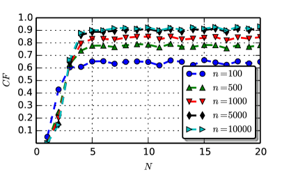
Figure 3: Efficiency of motion (as quantified by the chemotactic factor $CF$) as function of the number of arms $N$ for different simulation time steps $n$.

Next, we analyzed the influence of the cell geometry on the efficiency of motion. As Fig. 4 shows, $CF$ depends on the geometry of the cell characterized by the ratio $R_{l}/R_{s}$. Thus, more elongated cells (with $R_{l}>R_{s}$) have a higher $CF$. This is somewhat surprising as these cells have a broader force distribution than less elongated cells. However, as we show in Sup $CF$ depends predominantly on the ability of the cell to align with the prescribed gradient. Thus, for more elongated cells this higher ability compensates for the broader force distribution. The $CF$ as determined by the ability to align with the gradient (characterized by a rotational rate $\alpha$) is given by Sup

$$CF=\exp(x^{2})\left[\textup{erf}\left(\pi/(\sqrt{2}\sigma_{\theta})-x\right)+\textup{erf}(x)\right].$$ (4)

Here, $x=2^{-1/2}\sigma_{\theta}\alpha/\chi$ and the opening angle of the force distribution $\chi=\arctan\left(R_{l}/R_{s}\tan\sigma_{+}\right)$ parameterizes the dependence on cell geometry.

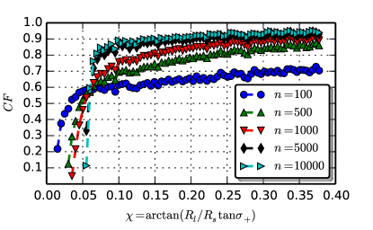
Figure 4: Chemotactic factor $CF$ is shown as function of cell geometry characterized by $R_{l}/R_{s}$. More elongated cells follow with higher efficiency the gradient (of strength $c_{0}=1/R_{l}$). The data shown are for different simulation time steps $n$. For smaller $n$ (i.e. earlier simulation times), $CF$ still depends on the initial alignment of the cells. With increasing $n$ the cells align with the gradient increasing in this way $CF$. However, as can be seen only cells with $\chi>0.06$ (i.e. cells which are sufficiently elongated) are able to align with the gradient.

Lo et. al. Lo et al. (2000) have shown that non-moving cells grow longer protrusions on stiff substrates than they do on soft substrates. This implies a regulative effect of the substrate rigidity. To account for this effect in our model we assign each arm $i$ the length

$$l_{i}+\delta l_{i}\left(c\right)=l_{i}+\frac{\delta l_{\mathrm{max}}}{1+\frac{k_{c}}{c}},$$ (5)

where the regulated elongation $\delta l_{i}\left(c\right)$ depends on the stiffness (or concentration or adhesiveness) $c=c\left(\bm{r}_{\mathrm{arm}}\right)$ at the position of the arm $\bm{r}_{\mathrm{arm}}$.

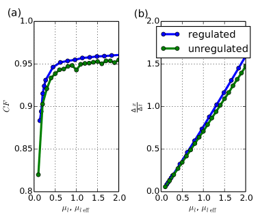
Figure S5: Effect of the concentration dependent regulation of arm lengths on efficiency of motion. (a) If we increase the average arm length $\mu_{l}$ we see an increase in efficiency that saturates for longer arms. If we use the concentration dependent regulation of arm lengths ($\mu_{l,\textup{eff}}$, see Eq. (5)) we get a 1% increase in maximum efficiency compared to the unregulated system from $CF\approx 0.95$ to $CF\approx 0.96$, but the same efficiency is reached with an average arm length up to 40% shorter compared to the unregulated system. (b) Speed of motion, characterized by the covered path length $\Delta x$ per time unit $\Delta t$ increases with increasing arm length. Additionally, for identical average arm length motion is faster with regulation. The difference in speed increases with increasing average arm length.

If we increase the average arm length, we see an increase in efficiency that saturates for longer arms, see Fig. S5 in Sup . This rise in efficiency comes with an increase in speed. If we use the concentration-dependent regulation of arm lengths we see a 1% increase in maximum efficiency compared to the unregulated system, but the same efficiency is reached with an average arm length up to 40% shorter compared to the unregulated system.

The above results are robust with respect to variations in the standard deviations of the distributions for $\varphi$ and $\gamma$. $CF$ remains nearly constant for $\sigma_{+}$ and $\sigma_{\gamma}$ in a range from $\sim 0.01\pi$ to $0.2\pi$. For even broader distributions we see a decrease in efficiency as a result of insufficient polarization of the cell. Experimentally, it has been observed that the protrusions grow almost in the normal direction out of the surface of the cells, and that the protrusions are located around a narrow region at the leading pole Maly and Borisy (2001); Svitkina et al. (2003); Mogilner and Rubinstein (2005); Parsons et al. (2010). We find a similar behavior (and the associated high efficiencies in motion) only for distributions with small standard deviations indicating that $\varphi$ and $\gamma$ are tightly regulated.

Furthermore, cell motion shows an interesting dependence on the position of the anchor point of the cell to the substrate quantified by the parameter $\delta$. If this point is shifted towards the leading pole, i.e. closer to the protrusions at the front, the torque exerted by these arms is reduced due to the shorter lever arm and the efficiency drops sharply to zero indicating that the cell is not able to follow the gradient at all (see Fig. 5). This indicates that the efficiency in following a gradient is dominated by protrusions close to the leading pole.

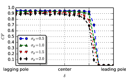
Figure 5: Dependence of $CF$ on the position of the anchor point to the substrate. The distance of this point from the center of the ellipse is denoted by $\delta$. As this point moves from the center of the ellipse towards the leading pole, $CF$ drops sharply to zero. This indicates that in order to be able to follow a prescribed gradient the cells need to have a defined leading pole and an anchor point sufficiently far away from this pole.

Cells often encounter inhomogeneous substrates. As a general scenario, we analyze the movement towards a step in substrate rigidity where crawling cells show an interesting behavior. At these steps (that could represent the transition from a rigid stroma of a tumor to the softer surroundings Butcher et al. (2009)) cells tend to move from the softer substrate to the stiffer substrate Bordeleau et al. (2013).

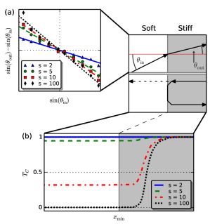
Figure 6: Transition at a sharp step. (a) If cells move from the soft region to the stiff region one finds a refractive behavior depending on the step size $s$. (b) Cells moving from the stiff to the soft region experience a barrier that they overcome with a step-size-dependent transmission coefficient. For large step sizes no cells cross the barrier while for small step sizes almost all cells are able to cross it.

Cells moving in this direction are only weakly influenced by the step. They keep moving but their trajectory bends towards the direction perpendicular to the step, see Fig. 6. We observed that the relation between the angle of the cell before and after the step obeys a refraction law similar to that of light allowing us to characterize the motion by refraction indices, see Fig. 6(a). The ratio of refraction indices ${n_{\mathrm{Soft}}}/{n_{\mathrm{Stiff}}}=\sin\theta_{\mathrm{o}ut}/\sin\theta_{\mathrm{i}n}$ decreases with increasing step size $s=c_{1}/c_{0}$, where $c_{0}$ and $c_{1}$ are the stiffness of the softer and stiffer region, respectively.

On the other hand, a step from a stiff substrate to a softer substrate represents a barrier for cells. The passing probability depends on the step height. From the distribution of the minimal $x$-positions encountered by the cells during 500 iterations, we can calculate the probability of a cell moving across the step, which we define as transmission coefficient $T_{\mathrm{C}}=\int_{-\infty}^{x_{\mathrm{step}}}p\left(x\right)=p\left(x<x_{\mathrm{step}}\right)$, where $p\left(x\right)$ is the probability to find a cell that traveled to position $x$, and $x_{\mathrm{step}}$ is the position of the step, see Fig. 6(b). This coefficient decreases as the step size increases showing that the barrier effect becomes much stronger for larger steps, see Fig. S7 in Sup .

Finally, we wanted to compare our results with other types of cellular motion. However, there are neither theoretical nor experimental data available for the efficiency of mammalian cell motion as function of gradient strength. We therefore decided to compare our model with data for swim-tumble chemotaxis, the standard model for cellular motion. More specifically we tested our results against a two-dimensional swim-tumble model for bacterial chemotaxis with a parameter set optimized for efficiency Macnab and Koshland (1972); Tindall et al. (2008a); Sup . As Fig. 7 shows our model yields significantly higher efficiencies than the swim-tumble model.

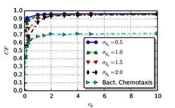
Figure 7: Variation of the efficiency with the gradient strength $c_{0}$. The cells reach their maximum efficiency at rather small gradients compared to a swim-tumble model of bacterial chemotaxis (based on Macnab and Koshland (1972); Tindall et al. (2008a)).

To summarize, in this study we have introduced a generic mechanical model for environment-sensitive motion of mammalian cells. Motion occurs by polarized growth of protrusions which push and rotate the cell. The description of molecular interactions occurs on a coarse-grained level effectively entering into the probability distribution for arm growth, see Eq. (1). It is not the goal of this simplified model to achieve a detailed (molecular) description of cellular motility. Rather, we introduce it to analyze the influence of mechanical forces on the regulation of fibroblast motion.

The agreement of our findings with the experimental observations indicates that mechanical forces indeed play a significant role in this process. More specifically, the observed high efficiency in following a gradient is a robust feature of our model (see figs. 4 and 7). We find for a large parameter range chemotactic factors close to 1 as observed experimentally in Theveneau et al. (2010). Furthermore, the results on the motion in inhomogeneous environments are in good agreement with the experimental observations at steps in substrate rigidity Bordeleau et al. (2013).

Our analysis identifies two geometrical factors that have a significant impact on efficiency of cell motion: the position of the anchor point and the geometry of cell quantified by the ratio of major to minor radius. For both quantities we make specific theoretical predictions (figs. 4 and 5) that are experimentally testable.

Furthermore, the moments $\langle x\rangle$, $\langle x^{2}\rangle$, $\langle y\rangle$ and $\langle y^{2}\rangle$ can be easily measured for individual cells of different geometry for different gradients. By comparing these data with our theoretical predictions (Fig. 7 and Figs. S5 and S6 in Sup ) information can be obtained about the concentration dependent regulation of arm lengths. To check our results concerning steps in concentration, adhesiveness and stiffness, one could use the methods presented in Bordeleau et al. (2013) to produce flat substrates of different stiffness and measure the polarization axes of the cells before and after the interface as well as the transmission coefficients with time-lapse microscopy.

There are many possible extensions of our model. In future work we will take into account the mechanical effects that the cells have on the substrate. If cells attach protrusions to the substrate and contract, they locally stiffen the substrate. This local stiffening of the substrate might lead to an effective attraction between two cells in proximity, in this way promoting aggregation.

Supplemental Material: A mechanical model for guided motion of mammalian cells

S Analytical results

S.1 Force distribution

The cell is represented by an ellipse with semiaxis $R_{l}\geq R_{s}$ (see Fig. S1). An adhesive arm grows out of the ellipse at angle $\varphi$. We now choose a coordinate system $\left(x^{\textup{sa}},y^{\textup{sa}}\right)$ with the fixed counterpart of the protrusions as origin and the semimajor axis as abscissa. The vector to the origin of an arbitrary arm is given by

$$\bm{r}_{\textup{arm}}=\left(\begin{array}[]{c}R_{l}~{}(\cos\varphi-\delta)\\ R_{s}\sin\varphi\end{array}\right).$$ (S.1)

The angle between the vector to the attachment point and the abscissa is

$$\varphi^{\prime}=\arctan\left(\frac{R_{s}\sin(\varphi)}{R_{l}~{}(\cos\varphi-\delta)}\right).$$ (S.2)

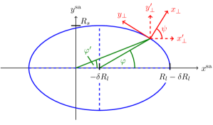
Figure S1: Ellipse in the coordinate system with fixed counterpart of the protrusions as origin and the semimajor axis as abscissa. Vectors to the attachment point from the origin and from the center of the ellipse are shown in green. The coordinate systems in the attachment point are shown in red: solid lines for the system with one axis perpendicular to the surface, dashed lines for the system rotated parallel to the system of the semiaxis.

Length $l$ and direction $\gamma$ of the arms are Gaussian distributed

$$p(\gamma)=\frac{1}{\sqrt{2\pi}\sigma_{\gamma}}\exp\left[-\frac{1}{2}\left(\frac{\gamma}{\sigma_{\gamma}}\right)^{2}\right],\quad p(l)=\frac{1}{\sqrt{2\pi}\sigma_{l}}\exp\left[-\frac{1}{2}\left(\frac{l-\overline{l}}{\sigma_{l}}\right)^{2}\right].$$ (S.3)

Here, the angle $\gamma$ is measured relative to the normal of the ellipse in the attachment point. The probability to find an arm with length $l$ and angle $\gamma$ is

$$p(l,\gamma)=p(l)p(\gamma)=\frac{1}{\sqrt{2\pi}\sigma_{\gamma}}\exp\left[-\frac{1}{2}\left(\frac{\gamma}{\sigma_{\gamma}}\right)^{2}\right]\frac{1}{\sqrt{2\pi}\sigma_{l}}\exp\left[-\frac{1}{2}\left(\frac{l-\overline{l}}{\sigma_{l}}\right)^{2}\right].$$ (S.4)

The force caused by an arm with length $l$ and angle $\gamma$ is given by

$$\bm{F}^{\perp}=kl\left(\begin{array}[]{c}\cos\gamma\\ \sin\gamma\end{array}\right)\equiv\left(\begin{array}[]{c}F^{\perp}_{x}\\ F^{\perp}_{y}\end{array}\right),$$ (S.5)

in the coordinate system $(x_{\perp},y_{\perp})$ in the attachment point (see Fig. S1). In the absence of a gradient we can assume $k=1$.

The probability to have a force $(F^{\perp}_{x},F^{\perp}_{y})$ is

$$p^{\perp}(F^{\perp}_{x},F^{\perp}_{y})=\frac{1}{2\pi\sigma_{l}\sigma_{\gamma}}\frac{1}{\sqrt{{F^{\perp}_{x}}^{2}+{F^{\perp}_{y}}^{2}}}\exp\left[-\frac{1}{2}\left(\frac{\sqrt{{F^{\perp}_{x}}^{2}+{F^{\perp}_{y}}^{2}}-\overline{l}}{\sigma_{l}}\right)^{2}\right]\exp\left[-\frac{1}{2}\left(\frac{\arctan(F^{\perp}_{y},F^{\perp}_{x})}{\sigma_{\gamma}}\right)^{2}\right],$$ (S.6)

where we denote by $\arctan(u,v)$ the arc tangent of $\frac{u}{v}$ taking into account the quadrant of the point $(u,v)$.

To get the force in the coordinate system of the semiaxes, we need to rotate by the angle

$$\psi=\arctan\left(R_{l}\sin\varphi,R_{s}\cos\varphi\right).$$ (S.7)

Thus,

$$p_{\varphi}^{\textup{sa}}(F_{x},F_{y}) =p_{\varphi}^{\perp}(F^{\perp}_{x},F^{\perp}_{y})\equiv p^{\perp}(F_{x}~{}\cos\psi+F_{y}~{}\sin\psi,-F_{x}~{}\sin\psi+F_{y}~{}\cos\psi)$$

$$=\frac{1}{2\pi\sigma_{l}\sigma_{\gamma}}\frac{1}{\sqrt{F_{x}^{2}+F_{y}^{2}}}\exp\left[-\frac{1}{2}\left(\frac{\sqrt{F_{x}^{2}+F_{y}^{2}}-\overline{l}}{\sigma_{l}}\right)^{2}\right]$$

$$\times\exp\left[-\frac{1}{2}\left(\frac{\arctan(-F_{x}~{}R_{l}~{}\sin\varphi+F_{y}~{}R_{s}~{}\cos\varphi,F_{x}~{}R_{s}~{}\cos\varphi+F_{y}~{}R_{l}~{}\sin\varphi)}{\sigma_{\gamma}}\right)^{2}\right].$$ (S.8)

This probability density is valid for any (fixed) $\varphi$. The complete density is given by

$$p^{\textup{sa}}(F_{x},F_{y}) =\int\limits_{-\pi}^{\pi}d\varphi~{}p_{\varphi}^{\textup{sa}}(F_{x},F_{y})~{}p(\varphi),$$ (S.9)

which has to be calculated numerically. The result shown in Fig. S2 is in good agreement with the numerical data.

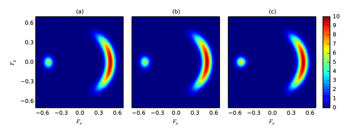
Figure S2: Probability density for the force $(F_{x},F_{y})$. (a) Numerical result; (b) analytical result (S.9) (for same set of parameters); (c) analytical result in the approximation (S.10).

As Fig. S2 shows the distributions of $\gamma$ and $\varphi$ are rather sharp (i.e. $\sigma_{\varphi-}<\sigma_{\gamma}\ll 1$). Therefore, we can approximate the corresponding Gaussian functions by delta functions leading to

$$p^{\textup{sa}}(F_{x},F_{y}) \approx\frac{p_{+}}{2\pi\sigma_{l}\sigma_{\varphi+}}\frac{R_{l}~{}R_{s}~{}\sqrt{F_{x}^{2}+F_{y}^{2}}}{R_{l}^{2}F_{x}^{2}+R_{s}^{2}F_{y}^{2}}\exp\left[-\frac{1}{2}\left(\frac{\sqrt{F_{x}^{2}+F_{y}^{2}}-\overline{l}}{\sigma_{l}}\right)^{2}\right]\exp\left[-\frac{1}{2}\left(\frac{\arctan\left(R_{s}~{}F_{y},R_{l}~{}F_{x}\right)}{\sigma_{\varphi+}}\right)^{2}\right]$$

$$+\frac{p_{-}}{2\pi\sigma_{l}\sigma_{\gamma}}\frac{1}{\sqrt{F_{x}^{2}+F_{y}^{2}}}\exp\left[-\frac{1}{2}\left(\frac{\sqrt{F_{x}^{2}+F_{y}^{2}}-\overline{l}}{\sigma_{l}}\right)^{2}\right]\exp\left[-\frac{1}{2}\left(\frac{\arctan\left(-F_{y},-F_{x}\right)}{\sigma_{\gamma}}\right)^{2}\right].$$ (S.10)

From this approximation, we conclude that the width of the distribution is given by $\sigma_{l}$ in radial direction and by $\sigma_{\varphi+}$ and $\sigma_{\gamma}$ in angular direction. We define $\chi$ as the angle, for which $\arctan\left(R_{s}~{}F_{y},R_{l}~{}F_{x}\right)\leq\sigma_{\varphi+}$, i.e.

$$\chi=\arctan\left(\frac{R_{l}}{R_{s}}~{}\tan\sigma_{\varphi+}\right).$$ (S.11)

Thus, $\chi$ quantifies the ability of the cell to move straight ahead and/or turn towards a given gradient. It depends on $\sigma_{\varphi+}$ and on the geometric factor $\frac{R_{l}}{R_{s}}$.

S.2 Model for motion along gradients

To investigate the influence of the opening angle on the ability to follow a gradient we analyze a somewhat simplified scenario: we neglect all effects from the back of the cell and do not take into account the torque.

In a first step we describe the motion as a random walk. In doing so we keep track of the position and direction of cell. In each step the cell follows its direction for a constant distance and then changes direction by an angle $\pm\eta$ relative to its current direction. The probabilities for selecting $+\eta$ and $-\eta$ are denoted by $p$ and $1-p$, respectively. The probability that after $N$ steps the cell is rotated $n$ times by $\eta$ and $N-n$ times by $-\eta$ (resulting in a net rotation of $(2n-N)\eta$) is given by

$$P_{N}(n) =\binom{N}{n}~{}p^{n}~{}(1-p)^{N-n}.$$ (S.12)

For large numbers ($N\gg 1$, $n\gg 1$, $N-n\gg 1$) this becomes a continuous Gaussian distribution for the net rotation $x=(2n-N)\eta$

$$P(x) =\frac{1}{\sqrt{2\pi}\sigma}\exp\left[-\frac{1}{2}\frac{\left(x-\overline{x}\right)^{2}}{\sigma^{2}}\right],$$ (S.13)

with mean $\overline{x}=N(2p-1)\eta$ and standard deviation $\sigma=2\sqrt{Np(1-p)}\eta$.

The efficiency of the motion can be quantified by the expectation value of $\cos x$ which represents the fraction of the distance covered in the direction of a gradient in $x$-direction

$$\langle\cos x\rangle=\int\limits_{-\infty}^{\infty}dx~{}\cos x~{}\frac{1}{\sqrt{2\pi}\sigma}\exp\left(-\frac{1}{2}~{}\frac{x^{2}}{\sigma^{2}}\right)=\exp\left(-\frac{1}{2}\sigma^{2}\right).$$ (S.14)

In the last equation one can identify the standard deviation $\sigma$ with the opening angle $\chi$ of the force distribution. Thus, this simple model predicts that with increasing $\chi$ the efficiency should decrease. As can be seen from Fig. S3 this clearly contradicts our numerical findings. This indicates that the ability to follow the gradient is not determining the efficiency of motion. As we show now, it in fact depends crucially on the ability of the cell to align with the gradient.

To do so, we assume that initially the cell has an angle $\theta_{0}$ between its major axis and the applied linear gradient. With a probability $p$ the cell now rotates by an angle $\Psi$ towards the gradient. Thus, after $n=\frac{|\theta_{0}|}{\Psi}$ the cell is perfectly aligned with the gradient.

Here, the efficiency can be quantified by the averaged probability of the cells to align with the gradient

$$\int\limits_{-\pi}^{\pi}d\theta_{0}~{}p^{\frac{|\theta_{0}|}{\Psi}}=2~{}\frac{\Psi}{\ln p}~{}\left[\exp\left(\frac{\pi}{\Psi}~{}\ln p\right)-1\right].$$ (S.15)

Taking into account that the starting angles $\theta_{0}$ are Gaussian distributed in our simulations, the efficiency becomes

$$\int\limits_{-\pi}^{\pi}d\theta_{0}\frac{1}{\sqrt{2\pi}\sigma_{\theta}}~{} \exp\left(-\frac{1}{2}~{}\frac{\theta_{0}^{2}}{\sigma_{\theta}^{2}}\right)~{}p^{\frac{|\theta_{0}|}{\Psi}}=\frac{2}{\sqrt{2\pi}\sigma_{\theta}}~{}\int\limits_{0}^{\pi}d\theta_{0}~{}\exp\left(-\frac{1}{2}~{}\frac{\theta_{0}^{2}}{\sigma_{\theta}^{2}}+\frac{\theta_{0}}{\Psi}~{}\ln p\right)$$

$$=\exp\left[\frac{\sigma_{\theta}^{2}~{}(\ln p)^{2}}{2~{}\Psi^{2}}\right]~{}\left\{\textup{erf}\left[\frac{1}{\sqrt{2}\sigma_{\theta}}~{}\left(\pi-\frac{\sigma_{\theta}^{2}~{}\ln p}{\Psi}\right)\right]+~{}\textup{erf}\left[~{}\left(\frac{\sigma_{\theta}~{}\ln p}{\sqrt{2}~{}\Psi}\right)\right]\right\}.$$ (S.16)

Thus, the probability depends on the rotation angle $\Psi$ (that we identify with the opening angle $\chi$ of the force distribution) and on the probability $p$ (which depends on the strength of the gradient). Because the exact relation between $p$ and the strength of the gradient is not known we take $\ln p$ as a fitting parameter. As one can see from Fig. S3 the fitted curves match the numerical data quite well for sufficiently large number of simulation steps. At early simulation stages the numerical data depends still on the initial orientation of the cell.

For vertically elongated cell ($R_{s}>2R_{l}$) the gradient eventually turns the cell into the “wrong” direction. This tilt in the wrong direction increases with time since arms growing in this direction are favored by the gradient. This process leads to an alignment of the ellipse against the gradient. We stopped our simulations when such an event occurred.

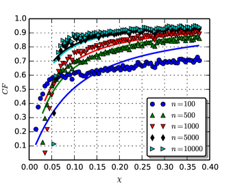
Figure S3: Efficiency of motion as function of $\chi$ and number of time steps $n$ in the simulation. At early simulation stages the efficiency is dominated by the alignment with the gradient. At later times all cells are aligned with the gradient and the efficiency approaches 1. For vertically elongated ellipses ($R_{s}>2R_{l}$) the torque can turn the cell against the gradient resulting in a negative efficiency. If this event occurred the simulation was stopped. The lines show the results of fitting Eq. (S.16) to the numerical data.

S Model for Bacterial Chemotaxis

To model the bacterial chemotaxis, we use the well-studied swim-tumble model. The cell swims into a random direction for a normally distributed length $l$. It measures the change in concentration $\Delta c$ of an attractant along this path. On the basis of $\Delta c$ the decision is made whether the cell maintains the current direction or tumbles. The former occurs with probability

$$p\left(\Delta c\right)=\left\{\begin{matrix}\dfrac{p_{0}}{1-\dfrac{\Delta c(1-p_{0})^{2}}{kp_{0}}}&\Delta c\leq 0\\ \dfrac{1}{1+\dfrac{k(1-p_{0})}{\Delta c+p_{0}(k-\Delta c)}}&\Delta c>0\end{matrix}\right.$$ (S.17)

which is larger than a basal probability of $p\left(\Delta c=0\right)=p_{0}$ for $\Delta c>0$ and smaller than $p_{0}$ for $\Delta c<0$. The parameter $k$ quantifies the stiffness of the response.

To compare this model with our model, we also applied here a concentration gradient with a linear slope in $x$-direction.

S Supplementary Figures

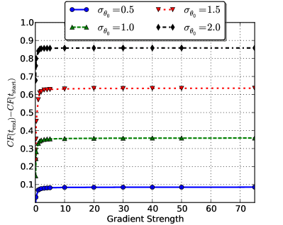
Figure S4: Gains in chemotactic factor $CF$, i.e. difference between $CF$ at the end and at the beginning of the simulation, as function of gradient strength $c_{0}$. Results are shown for different standard deviations $\sigma_{\theta}$ of the initial polarization angle $\theta_{0}$. For smaller $\sigma_{\theta}$ the cells are initially aligned more in the direction of the gradient, so less gain is expected.

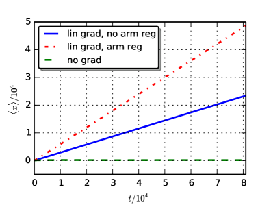
Figure S6: Classification of the migration dynamics. The cell performs a random walk which is biased in the presence of a gradient, see Fig. 2. If the arms are regulated the motion in absence of a gradient stays the same, whereas the motion in presence of a gradient becomes faster at constant efficiency (additional red dash-dotted line).

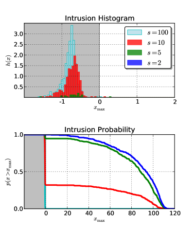
Figure S7: Histogram and probability of intrusion at a surface step (i.e. interface between stiff and soft substrate region). Cells move from left (grey, stiff substrate) to right (white, soft substrate). The histogram shows the frequency of the maximal (most right) $x$ value reached. We only show the region close to the step to focus on the cells that did not cross it. Cells that have passed the step (most of the cells in simulations for small steps, i.e. blue and green) would be found at $x_{\textup{max}}>2$, so they are not shown in the histogram. For larger step sizes not all cells pass the step. The maximal distance traveled in positive $x$-direction peaks closer to the interface with decreasing step size. If the step size becomes too small almost all cells pass the step as indicated by the intrusion probability that is defined as the probability that a cell travels further than $x_{\textup{max}}$.

S Supplementary Tables

Parameter	Fig. 2 & S6	Fig. 3	Fig. 4 & S3	Fig. 5	Fig. 6(a)	Fig. 6(b)	Fig. 7	Fig. S2	Fig. S4	Fig. S6	Fig. S7
Iter.	81000	–	–	500	500	500	500	1	500	500	500
Runs	500	500	1000	500	500	500	500	5000000	500	500	500
$a$	1	1	1	1	1	1	1	1	1	1	1
$b$	0.5	0.5	–	0.5	0.5	0.5	0.5	0.5	0.5	0.5	0.5
$\delta$	-1	-1	-0.9	–	-1	-1	-1	-0.9	-1	-1	-1
$\sigma_{\theta}$	1.047	1.047	1.047	–	–	0	1.047	–	–	1.047	0
$k$	1	1	1	1	1	1	1	1	1	1	1
$c_{0}$	–	1	1	1	1	1	1	–	–	1	1
$N$	10	–	10	10	10	10	10	1	10	10	10
$p_{+}$	0.9	0.9	0.9	0.9	0.9	0.9	0.9	0.9	0.9	0.9	0.9
$\mu_{l}$	0.5	0.5	0.5	0.5	0.5	0.5	0.5	0.5	0.5	–	0.5
$\sigma_{l}$	0.05	0.05	0.05	0.05	0.05	0.05	0.05	0.05	0.05	0.05	0.05
$\sigma_{+}$	0.5	0.1	0.1	0.5	0.5	0.5	0.5	0.3	0.5	0.5	0.5
$\sigma_{-}$	0.05	0.01	0.01	0.05	0.05	0.05	0.05	0.03	0.05	0.05	0.05
$\sigma_{\gamma}$	0.7	0.1	0.1	0.1	0.1	0.1	0.1	0.1	0.1	0.1	0.1

Table S1: Parameter values for the results shown in Figs. 2-7, S2-S7

Step size $s$	$\frac{n_{\mathrm{Soft}}}{n_{\mathrm{Stiff}}}$	$T_{\mathrm{C}}$
2	0.9374	1.0000
5	0.8843	0.9480
10	0.8622	0.3220
100	0.8330	0.0020

Table S2: Values for the ratio of refraction indices $\frac{n_{\mathrm{Soft}}}{n_{\mathrm{Stiff}}}$ and transmission coefficient $T_{\mathrm{C}}$. The refractive effect becomes stronger with increasing step size whereas the transmission decreases.

References

- Chicurel (2002) M. Chicurel, Science 295, 606 (2002).
- Gray et al. (2003) D. Gray, J. Tien, and C. Chen, J. Biomed. Mater. Res. 66, 605 (2003).
- Huttenlocher and Horwitz (2011) A. Huttenlocher and A. R. Horwitz, Cold Spr. Harbor Perspec. Biol. 3, a005074 (2011).
- Prost et al. (2008) J. Prost, J.-F. Joanny, P. Lenz, and C. Sykes, The physics of Listeria Propulsion in Cell Motility, edited by P. Lenz (2008).
- Parsons et al. (2010) J. T. Parsons, A. R. Horwitz, and M. A. Schwartz, Nat. Rev. Mol. Cell Biol. 11, 633 (2010).
- Lo et al. (2000) C. M. Lo, H. B. Wang, M. Dembo, and Y. L. Wang, Biophys. J. 79, 144 (2000).
- Gerisch and Chaplain (2008) A. Gerisch and M. A. J. Chaplain, J. Theor. Biol. 250, 684 (2008).
- Bordeleau and Galarneau (2010) F. Bordeleau and L. Galarneau, Mol. Biol. Cell 21, 1698 (2010).
- Macnab and Koshland (1972) R. Macnab and D. Koshland, Proc. Natl Acad. Sci. USA 69, 2509 (1972).
- Tindall et al. (2008a) M. J. Tindall, P. K. Maini, S. L. Porter, and J. P. Armitage, Bull. Math. Biol. 70, 1570 (2008a).
- Levine and Rappel (2008) H. Levine, and W.-J. Rappel, Directed Motility and Dictyostelium Aggregation in Cell Motility, edited by P. Lenz (2008).
- Carter (1965) S. B. Carter, Nature (London) 208, 1183 (1965).
- Tindall et al. (2008b) M. J. Tindall, S. L. Porter, P. K. Maini, G. Gaglia, and J. P. Armitage, Bull. Math. Biol. 70, 1525 (2008b).
- Adler (1966) J. Adler, Science 153, 708 (1966).
- Adler (1975) J. Adler, Annu. Rev. Biochem. 44, 341 (1975).
- Tu et al. (2008) Y. Tu, T. S. Shimizu, and H. C. Berg, Proc. Natl Acad. Sci. USA 105, 14855 (2008).
- Zhu et al. (2012) X. Zhu, G. Si, N. Deng, Q. Ouyang, T. Wu, Z. He, L. Jiang, C. Luo, and Y. Tu, Phys. Rev. Lett. 108, 128101 (2012).
- Fisher et al. (1989) P. Fisher, R. Merkl, and G. Gerisch, J. Cell Biol. 108, 973 (1989).
- Fuller et al. (2010) D. Fuller, W. Chen, M. Adler, A. Groisman, H. Levine, W.-J. Rappel, and W. F. Loomis, Proc. Natl Acad. Sci. USA 107 (2010).
- Hecht et al. (2011) I. Hecht, M. L. Skoge, P. G. Charest, E. Ben-Jacob, R. A. Firtel, W. F. Loomis, H. Levine, and W.-J. Rappel, PLoS Comput. Biol 7, e1002044 (2011).
- Buenemann et al. (2010) M. Buenemann, H. Levine, W.-J. Rappel, and L. M. Sander, Biophys. J. 99, 50 (2010).
- Camley et al. (2013) B. A. Camley, Y. Zhao, B. Li, H. Levine, and W.-J. Rappel, Phys. Rev. Lett. 111, 158102 (2013).
- Zaman et al. (2005) M. H. Zaman, R. D. Kamm, P. Matsudaira, and D. A. Lauffenburger, Biophys. J. 89, 1389 (2005).
- Häcker (2012) A. Häcker, J. Math. Biol. 64, 361 (2012).
- Rubinstein et al. (2005) B. Rubinstein, K. Jacobson, and A. Mogilner, Multiscale Modeling & Simulation 3, 413 (2005).
- DiMilla et al. (1991) P. A. DiMilla, K. Barbee, and D. A. Lauffenburger, Biophys. J. 60, 15 (1991).
- Butcher et al. (2009) D. T. Butcher, T. Alliston, and V. M. Weaver, Nat. Rev. Cancer 9, 108 (2009).
- Theveneau et al. (2010) E. Theveneau, L. Marchant, S. Kuriyama, M. Gull, B. Moepps, M. Parsons, and R. Mayor, Dev. Cell 19, 39 (2010).
- Keren and Theriot (2008) K. Keren and J. A. Theriot, Biophysical Aspects of Actin-Based Cell Motility in Fish Epithelial Keratocytes in Cell Motility, edited by P. Lenz (2008).
- Mogilner (2009) A. Mogilner, J. Math. Biol. 58, 105 (2009).
- Lauffenburger and Horwitz (1996) D. A. Lauffenburger and A. F. Horwitz, Cell 84, 359 (1996).
- Pathak and Kumar (2011) A. Pathak and S. Kumar, PloS one 6, e18423 (2011).
- Ridley et al. (2003) A. J. Ridley, M. A. Schwartz, K. Burridge, R. A. Firtel, M. H. Ginsberg, G. Borisy, J. T. Parsons, and A. R. Horwitz, Science 302, 1704 (2003).
- Friedl (2004) P. Friedl, Curr. Opin. Cell Biol. 16, 14 (2004).
- Holmes and Edelstein-Keshet (2012) W. R. Holmes and L. Edelstein-Keshet, PLoS Comput. Biol 8, e1002793 (2012).
- Trichet et al. (2012) L. Trichet, J. Le Digabel, R. J. Hawkins, S. R. K. Vedula, M. Gupta, C. Ribrault, P. Hersen, R. Voituriez, and B. Ladoux, Proc. Natl Acad. Sci. USA 109, 6933 (2012).
- Provenzano et al. (2008) P. P. Provenzano, D. R. Inman, K. W. Eliceiri, S. M. Trier, and P. J. Keely, Biophys. J. 95, 5374 (2008).
- Yeung et al. (2005) T. Yeung, P. C. Georges, L. A. Flanagan, B. Marg, M. Ortiz, M. Funaki, N. Zahir, W. Ming, V. Weaver, and P. A. Janmey, Cell Motil. Cytoskeleton 60, 24 (2005).
- Bordeleau et al. (2013) F. Bordeleau, L. N. Tang, and C. A. Reinhart-King, Phys. Biol. 10, 065004 (2013).
- Levine and Rappel (2013) H. Levine and W.-J. Rappel, Phys. Today 66, 24 (2013).
- (41) See Supplemental Material for further information about analytical results and parameter values.
- Raucher and Sheetz (1999) D. Raucher and M. P. Sheetz, Biophys. J. 77, 1992 (1999).
- Baxter et al. (2002) L. C. Baxter, V. Frauchiger, M. Textor, I. Gwynn, and R. G. Richards, Eur. Cell. Mater. 4, 1 (2002).
- Maly and Borisy (2001) I. V. Maly and G. G. Borisy, Proc. Natl Acad. Sci. USA 98, 11324 (2001).
- Svitkina et al. (2003) T. M. Svitkina, E. A. Bulanova, O. Y. Chaga, D. M. Vignjevic, S.-I. Kojima, J. M. Vasiliev, and G. G. Borisy, J. Cell Biol. 160, 409 (2003).
- Mogilner and Rubinstein (2005) A. Mogilner and B. Rubinstein, Biophys. J. 89, 782 (2005).