Unconfused Ultraconservative Multiclass Algorithms

Abstract

We tackle the problem of learning linear classifiers from noisy datasets in a multiclass setting. The two-class version of this problem was studied a few years ago where the proposed approaches to combat the noise revolve around a Perceptron learning scheme fed with peculiar examples computed through a weighted average of points from the noisy training set. We propose to build upon these approaches and we introduce a new algorithm called UMA (for Unconfused Multiclass additive Algorithm) which may be seen as a generalization to the multiclass setting of the previous approaches. In order to characterize the noise we use the confusion matrix as a multiclass extension of the classification noise studied in the aforementioned literature. Theoretically well-founded, UMA furthermore displays very good empirical noise robustness, as evidenced by numerical simulations conducted on both synthetic and real data.

1 Introduction

Context.

This paper deals with linear multiclass classification problems defined on an input space $\mathcal{X}$ (e.g., $\mathcal{X}=\mathbb{R}^{d}$) and a set of classes

$${\cal Q}\doteq\{1,\ldots,Q\}.$$

In particular, we are interested in establishing the robustness of ultraconservative additive algorithms crammer03ultraconservative to label noise classification in the multiclass setting—in order to lighten notation, we will now refer to these algorithms as ultraconservative algorithms. We study whether it is possible to learn a linear predictor from a training set made of independent realizations of a pair $(X,Y)$ of random variables:

$$\mathcal{S}\doteq\{(\bm{x}_{i},y_{i})\}_{i=1}^{n}$$

where $y_{i}\in{\cal Q}$ is a corrupted version of a true label, i.e. deterministically computed class, $t(\bm{x}_{i})\in{\cal Q}$ associated with $\bm{x}_{i}$, according to some concept $t$. The random noise process $Y$ that corrupts the label to provide the $y_{i}$’s given the $\bm{x}_{i}$’s is supposed uniform within each pair of classes, thus it is fully described by a confusion matrix $C=(C_{pq})_{p,q}\in\mathbb{R}^{Q\times Q}$ so that

$$\forall\bm{x},C_{pt(\bm{x})}=\mathbb{P}_{Y}(Y=p|\bm{x}).$$

The goal that we would like to achieve is to provide a learning procedure able to deal with the confusion noise present in the training set $\mathcal{S}$ to give rise to a classifier $h$ with small risk

$$R(h)\doteq\mathbb{P}_{X\sim\mathcal{D}}(h(X)\neq t(X)),$$

$\mathcal{D}$ being the distribution according to which the $\bm{x}_{i}$’s are obtained. As we want to recover from the confusion noise, i.e., we want to achieve low risk on uncorrupted/non-noisy data, we use the term unconfused to characterize the procedures we propose.

Ultraconservative learning procedures are online learning algorithms that output linear classifiers. They display nice theoretical properties regarding their convergence in the case of linearly separable datasets, provided a sufficient separation margin is guaranteed (as formalized in Assumption 1 below). In turn, these convergence-related properties yield generalization guarantees about the quality of the predictor learned. We build upon these nice convergence properties to show that ultraconservative algorithms are robust to a confusion noise process, provided that: i) $C$ is invertible and can be accessed, ii) the original dataset $\{(\bm{x}_{i},t(\bm{x}_{i}))\}_{i=1}^{n}$ is linearly separable. This paper is essentially devoted to proving how/why ultraconservative multiclass algorithms are indeed robust to such situations. To some extent, the results provided in the present contribution may be viewed as a generalization of the contributions on learning binary perceptrons under misclassification noise blum96polynomialtime ; bylander94learning .

Beside the theoretical questions raised by the learning setting considered, we may depict the following example of an actual learning scenario where learning from noisy data is relevant. This learning scenario will be further investigated from an empirical standpoint in the section devoted to numerical simulations (Section 4).

Example 1

One situation where coping with mislabelled data is required arises in (partially supervised) scenarios where labelling data is very expensive. Imagine a task of text categorization from a training set $\mathcal{S}=\mathcal{S}_{\ell}\operatorname*{\cup}\mathcal{S}_{u}$, where $\mathcal{S}_{\ell}=\{(\bm{x}_{i},y_{i})\}_{i=1}^{n}$ is a set of $n$ labelled training examples and $\mathcal{S}_{u}=\{\bm{x}_{n+i}\}_{i=1}^{m}$ is a set of $m$ unlabelled vectors; in order to fall back to realistic training scenarios where more labelled data cannot be acquired, we may assume that $n\ll m$. A possible three-stage strategy to learn a predictor is as follows: first learn a predictor $f_{\ell}$ on $\mathcal{S}_{\ell}$ and estimate its confusion error $C$ via a cross-validation procedure—$f$ is assumed to make mistakes evenly over the class regions—, second, use the learned predictor to label all the data in $\mathcal{S}_{u}$ to produce the labelled traning set $\widehat{\mathcal{S}}=\{(\bm{x}_{n+i},t_{n+i}:=f(\bm{x}_{n+i}))\}_{i=1}^{m}$ and finally, learn a classifier $f$ from $\widehat{\mathcal{S}}$ and the confusion information $C$.

This introductory example pertains to semi-supervised learning and this is only one possible learning scenario where the contribution we propose, UMA, might be of some use. Still, it is essential to understand right away that one key feature of UMA, which sets it apart from many contributions encountered in the realm of semi-supervised learning, is that we do provide theoretical bounds on the sample complexity and running time required by our algorithm to output an effective predictor.

The present paper is an extended version of LoucheR13ACML . Compared with the original paper, it provides a more detailed introduction of the tools used in the paper, a more thorough discussion on related work as well as more extensive numerical results (which confirm the relevance of our findings). A strategy to make use of kernels for nonlinear classification has also been added.

Contributions.

Our main contribution is to show that it is both practically and theoretically possible to learn a multiclass classifier on noisy data if some information on the noise process is available. We propose a way to generate new points for which the true class is known. Hence we can iteratively populate a new unconfused dataset to learn from. This allows us to handle a massive amount of mislabelled data with only a very slight loss of accuracy. We embed our method into ultraconservative algorithms and provide a thorough analysis of it, in which we show that the strong theoretical guarantees that characterize the family of ultraconservative algorithms carry over to the noisy scenario.

Related Work.

Learning from mislabelled data in an iterative manner has a long-standing history in the machine learning community. The first contributions on this topic, based on the Perceptron algorithm minsky69perceptrons , are those of bylander94learning ; blum96polynomialtime ; cohen97learning , which promoted the idea utilized here that a sample average may be used to construct update vectors relevant to a Perceptron learning procedure. These first contributions were focused on the binary classification case and, for blum96polynomialtime ; cohen97learning , tackled the specific problem of strong-polynomiality of the learning procedure in the probably approximately correct (PAC) framework kearns94introduction . Later, stempfel07learning proposed a binary learning procedure making it possible to learn a kernel Perceptron in a noisy setting; an interesting feature of this work is the recourse to random projections in order to lower the capacity of the class of kernel-based classifiers. Meanwhile, many advances were witnessed in the realm of online multiclass learning procedures. In particular, crammer03ultraconservative proposed families of learning procedures subsuming the Perceptron algorithm, dedicated to tackle multiclass prediction problems. A sibling family of algorithms, the passive-aggressive online learning algorithms crammer06online , inspired both by the previous family and the idea of minimizing instantaneous losses, were designed to tackle various problems, among which multiclass linear classification. Sometimes, learning with partially labelled data might be viewed as a problem of learning with corrupted data (if, for example, all the unlabelled data are randomly or arbitrarily labelled) and it makes sense to mention the works Kakade2008Banditron and RalaivolaFGBD11 as distant relatives to the present work.

Organization of the paper.

Section 2 formally states the setting we consider throughout this paper. Section 3 provides the details of our main contribution: the UMA algorithm and its detailed theoretical analysis. Section 4 presents numerical simulations that support the soundness of our approach.

2 Setting and Problem

2.1 Noisy Labels with Underlying Linear Concept

The probabilistic setting we consider hinges on the existence of two components. On the one hand, we assume an unknown (but fixed) probability distribution $\mathcal{D}$ on the input space $\mathcal{X}\doteq\mathbb{R}^{d}$. On the other hand, we also assume the existence of a deterministic labelling function $t:\mathcal{X}\to{\cal Q}$, where ${\cal Q}\doteq\{1,\ldots Q\}$, which associates a label $t(\bm{x})$ to any input example $\bm{x}$; in the Probably Approximately Correct (PAC) literature, $t$ is sometimes referred to as a concept kearns94introduction ; valiant84theory .

In the present paper, we focus on learning linear classifiers, defined as follows.

Definition 1 (Linear classifiers)

The linear classifier $f_{W}:\mathcal{X}\rightarrow{\cal Q}$ is a classifier that is associated with a set of vectors $W=[\bm{w}_{1}\cdots\bm{w}_{Q}]\in\mathbb{R}^{d\times Q}$, which predicts the label $f_{W}(\bm{x})$ of any vector $\bm{x}\in\mathcal{X}$ as

$$f_{W}(\bm{x})=\operatorname*{\text{argmax}\;}_{q\in{\cal Q}}\left\langle\bm{w}_{q},\bm{x}\right\rangle.$$ (1)

Additionally, without loss of generality, we suppose that

$$\mathbb{P}_{X\sim\mathcal{D}}\left(\left\|X\right\|=1\right)=1,$$

where $\|\cdot\|$ is the Euclidean norm. This allows us to introduce the notion of margin.

Definition 2 (Margin of a linear classifier)

Let $c:\mathcal{S}\rightarrow{\cal Q}$ be some fixed concept. Let $W=[\bm{w}_{1}\cdots\bm{w}_{Q}]\in\mathbb{R}^{d\times Q}$ be a set of $Q$ weight vectors. Linear classifier $f_{W}$ is said to have margin $\theta>0$ with respect to $c$ (and distribution $\mathcal{D}$) if the following holds:

$$\mathbb{P}_{X\sim\mathcal{D}}\left\{\exists p\neq c(X):\left\langle\bm{w}_{c(X)}-\bm{w}_{p},X\right\rangle\leq\theta\right\}=0.$$

Note that if $f_{W}$ has margin $\theta>0$ with respect to $c$ then

$$\mathbb{P}_{X\sim\mathcal{D}}(f_{W}(X)\neq c(X))=0.$$

Equipped with this definition, we shall consider that the following assumption of linear separability with margin $\theta$ of concept $t$ holds throughout.

Assumption 1 (Linear Separability of $t$ with Margin $\theta$.)

There exist $\theta\geq 0$ and $W^{*}=[\bm{w}_{1}^{*}\cdots\bm{w}_{Q}^{*}]\in\mathbb{R}^{d\times Q}$, with $\|W^{*}\|_{F}^{2}=1$ ($\|\cdot\|_{F}$ denotes the Frobenius norm) such that $f_{W^{*}}$ has margin $\theta$ with respect to the concept $t$.

In a conventional setting, one would be asked to learn a classifier $f$ from a training set

$$\mathcal{S}_{\text{true}}\doteq\{(\bm{x}_{i},t(\bm{x}_{i}))\}_{i=1}^{n}$$

made of $n$ labelled pairs from $\mathcal{X}\times{\cal Q}$ such that the $\bm{x}_{i}$’s are independent realizations of a random variable $X$ distributed according to $\mathcal{D}$, with the objective of minimizing the true risk or misclassification error $R_{\text{error}}(f)$ of $f$ given by

$$R_{\text{error}}(f)\doteq\mathbb{P}_{X\sim\mathcal{D}}(f(X)\neq t(X)).$$ (2)

In other words, the objective is for $f$ to have a prediction behavior as close as possible to that of $t$. As announced in the introduction, there is however a little twist in the problem that we are going to tackle. Instead of having direct access to $\mathcal{S}_{\text{true}}$, we assume that we only have access to a corrupted version

$$\mathcal{S}\doteq\{(\bm{x}_{i},y_{i})\}_{i=1}^{n}$$ (3)

where each $y_{i}$ is the realization of a random variable $Y$ whose distribution agrees with the following assumption:

Assumption 2

The law $\mathcal{D}_{Y|X}$ of $Y$ is the same for all $x\in\mathcal{X}$ and its conditional distribution

$$\mathbb{P}_{Y\sim\mathcal{D}_{Y|X=\bm{x}}}(Y|X=\bm{x})$$

is fully summarized into a known confusion matrix $C$ given by

$$\forall\bm{x},\;C_{pt(\bm{x})}\doteq\mathbb{P}_{Y\sim\mathcal{D}_{Y|X=\bm{x}}}(Y=p|X=\bm{x})=\mathbb{P}_{Y\sim\mathcal{D}_{Y|X=\bm{x}}}(Y=p|t(\bm{x})=q).$$ (4)

Alternatively put, the noise process that corrupts the data is uniform within each class and its level does not depend on the precise location of $\bm{x}$ within the region that corresponds to class $t(\bm{x})$. The noise process $Y$ is both a) aggressive, as it does not only apply, as we may expect, to regions close to the class boundaries between classes and b) regular, as the mislabelling rate is piecewise constant. Nonetheless, this setting can account for many real-world problems as numerous noisy phenomena can be summarized by a simple confusion matrix. Moreover it has been proved blum96polynomialtime that robustness to classification noise generalizes robustness to monotonic noise where, for each class, the noise rate is a monotonically decreasing function of the distance to the class boundaries.

Remark 1

The confusion matrix $C$ should not be mistaken with the matrix $\tilde{C}$ of general term: $\tilde{C}_{ij}\doteq\mathbb{P}_{X\sim\mathcal{D}_{X|Y=j}}(t(X)=i|Y=j)$ which is the class-conditional distribution of $t(X)$ given $Y$. The problem of learning from a noisy training set and $\tilde{C}$ is a different problem than the one we aim to solve. In particular, $\tilde{C}$ can be used to define cost-sensitive losses rather directly whereas doing so with $C$ is far less obvious. Anyhow, this second problem of learning from $\tilde{C}$ is far from trivial and very interesting, and it falls way beyond the scope of the present work.

Finally, we assume the following from here on:

Assumption 3

$C$ is invertible.

Note that this assumption is not as restrictive as it may appear. For instance, if we consider the learning setting depicted in Example 1 and implemented in the numerical simulations, then the confusion matrix obtained from the first predictor $f_{\ell}$ is often diagonally dominant, i.e. the magnitudes of the diagonal entries are larger than the sum of the magnitudes of the entries in their corresponding rows, and $C$ is therefore invertible. Generally speaking, the problems that we are interested in (i.e. problems where the true classes seems to be recoverable) tend to have invertible confusion matrix. It is most likely that invertibility is merely a sufficient condition on $C$ that allows us to establish learnability in the sequel. Identifying less stringent conditions on $C$, or conditions termed in a different way—which would for instance be based on the condition number of $C$—for learnability to remain, is a research issue of its own that we leave for future investigations.

The setting we have just presented allows us to view $\mathcal{S}=\{(\bm{x}_{i},y_{i})\}_{i=1}^{n}$ as the realization of a random sample $\{(X_{i},Y_{i})\}_{i=1}^{n}$, where each pair $(X_{i},Y_{i})$ is an independent copy of the random pair $(X,Y)$ of law $\mathcal{D}_{XY}\doteq\mathcal{D}_{X}\mathcal{D}_{X|Y}.$

2.2 Problem: Learning a Linear Classifier from Noisy Data

The problem we address is the learning of a classifier $f$ from $\mathcal{S}$ and $C$ so that the error rate

$$R_{\text{error}}(f)=\mathbb{P}_{X\sim\mathcal{D}}(f(X)\neq t(X))$$

of $f$ is as small as possible: the usual goal of learning a classifier $f$ with small risk is preserved, while now the training data is only made of corrupted labelled pairs.

Building on Assumption 1, we may refine our learning objective by restricting ourselves to linear classifiers $f_{W}$, for $W=[\bm{w}_{1}\cdots\bm{w}_{Q}]\in\mathbb{R}^{d\times Q}$ (see Definition 1). Our goal is thus to learn a relevant matrix $W$ from $\mathcal{S}$ and the confusion matrix $C$. More precisely, we achieve risk minimization through classic additive methods and the core of this work is focused on computing noise-free update points such that the properties of said methods are unchanged.

3 Uma: Unconfused Ultraconservative Multiclass Algorithm

This section presents the main result of the paper, that is, the UMA procedure, which is a response to the problem posed above: UMA makes it possible to learn a multiclass linear predictor from $\mathcal{S}$ and the confusion information $C$. In addition to the algorithm itself, this section provides theoretical results regarding the convergence and sample complexity of UMA.

As UMA is a generalization of the ultraconservative additive online algorithms proposed in crammer03ultraconservative to the case of noisy labels, we first and foremost recall the essential features of this family of algorithms. The rest of the section is then devoted to the presentation and analysis of UMA.

3.1 A Brief Reminder on Ultraconservative Additive Algorithms

Ultraconservative additive online algorithms were introduced by Crammer et al. in crammer03ultraconservative . As already stated, these algorithms output multiclass linear predictors $f_{W}$ as in Definition 1 and their purpose is therefore to compute a set $W=[\bm{w}_{1}\cdots\bm{w}_{Q}]\in\mathbb{R}^{d\times Q}$ of $Q$ weight vectors from some training sample $\mathcal{S}_{\text{true}}=\{(\bm{x}_{i},t(\bm{x}_{i}))\}_{i=1}^{n}$. To do so, they implement the procedure depicted in Algorithm 1, which centrally revolves around the identification of an error set and its simple update: when processing a training pair $(\bm{x},y)$, they perform updates of the form

$$\bm{w}_{q}\leftarrow\bm{w}_{q}+\tau_{q}\bm{x},\;q=1,\ldots Q,$$

whenever the error set ${\cal E}(\bm{x},y)$ defined as

$${\cal E}(\bm{x},y)\doteq\left\{r\in{\cal Q}\backslash\{y\}:\langle\bm{w}_{r},\bm{x}\rangle-\langle\bm{w}_{y},\bm{x}\rangle\geq 0\right\}$$ (5)

is not empty, with the constraint for the family $\{\tau_{q}\}_{q\in{\cal Q}}$ of step sizes to fulfill

$$\left\{\begin{array}[]{l}\tau_{y}=1\\ \tau_{r}\leq 0,\text{ if }r\in{\cal E}(\bm{x},y)\\ \tau_{r}=0,\text{ otherwise}\end{array}\right.\quad\text{ and }\quad\sum_{r=1}^{Q}\tau_{r}=0.$$ (6)

The term ultraconservative refers to the fact that only those prototype vectors $\bm{w}_{r}$ which achieve a larger inner product $\langle\bm{w}_{r},\bm{x}\rangle$ than $\langle\bm{w}_{y},\bm{x}\rangle$, that is, the vectors that can entail a prediction mistake when decision rule (1) is applied, may be affected by the update procedure. The term additive conveys the fact that the updates consist in modifying the weight vectors $\bm{w}_{r}$’s by adding a portion of $\bm{x}$ to them (which is to be opposed to multiplicative update schemes). Again, as we only consider these additive types of updates in what follows, it will have to be implicitly understood even when not explicitly mentioned.

Algorithm 1 Ultraconservative Additive algorithms crammer03ultraconservative .

0:  $\mathcal{S}_{\text{true}}$

0:  $W=\left[\bm{w}_{1},\ldots,\bm{w}_{Q}\right]$ and associated classifier $f_{W}(\cdot)=\operatorname*{\text{argmax}\;}_{q}\langle\bm{w}_{q},\cdot\rangle$

  Initialization: $\bm{w}_{q}\leftarrow 0,\;\forall q\in{\cal Q}$

  repeat

     access training pair $(\bm{x}_{t},y_{t})$

     compute the error set ${\cal E}(\bm{x}_{t},y_{t})$ according to (5)

     if ${\cal E}(\bm{x}_{t},y_{t})\neq\emptyset$ then

        compute a set $\{\tau_{q}\}_{q\in{\cal Q}}$ of update steps that comply with (6)

        perform the updates

$$\bm{w}_{q}\leftarrow\bm{w}_{q}+\tau_{q}\bm{x}_{q},\;\forall q\in{\cal Q}$$

     end if

  until some stopping criterion is met

One of the main results regarding ultraconservative algorithms, which we extend in our learning scenario is the following.

Theorem 3.1 (Mistake bound for ultraconservative algorithms crammer03ultraconservative .)

Suppose that concept $t$ is in accordance with Assumption 1. The number of mistakes/updates made by one pass over $\mathcal{S}$ by any ultraconservative procedure is upper-bounded by $2/\theta^{2}$.

This result is essentially a generalization of the well-known Block-Novikoff theorem block62perceptron ; novikoff63convrgence , which establishes a mistake bound for the Perceptron algorithm (an ultraconservative algorithm itself).

3.2 Main Result and High Level Justification

This section presents our main contribution, UMA, a theoretically grounded noise-tolerant multiclass algorithm depicted in Algorithm 2. UMA learns and outputs a matrix $W=[\bm{w}_{1}\cdots\bm{w}_{Q}]\in\mathbb{R}^{d\times Q}$ from a noisy training set $\mathcal{S}$ to produce the associated linear classifier

$$f_{W}(\cdot)=\operatorname*{\text{argmax}\;}_{q}\langle\bm{w}_{q},\cdot\rangle$$ (7)

by iteratively updating the $\bm{w}_{q}$’s, whilst maintaining $\sum_{q}\bm{w}_{q}=0$ throughout the learning process. As a new member of multiclass additive algorithms, we may readily recognize in step 8 through step 10 of Algorithm 2 the generic step sizes $\{\tau_{q}\}_{q\in{\cal Q}}$ promoted by ultraconservative algorithms (see Algorithm 1). An important feature of UMA is that it only uses information provided by $\mathcal{S}$ and does not make assumption on the accessibility to the noise-free dataset $\mathcal{S}_{\text{true}}$: the incurred pivotal difference with regular ultraconservative algorithms is that the update points used are now the computed (line 4 through line 7) $\bm{z}_{pq}$ vectors instead of the $\bm{x}_{i}$’s. Establishing that under some conditions UMA stops and provides a classifier with small risk when those update points are used is the purpose of the following subsections; we will also discuss the unspecified step 3, dealing with the selection step.

Algorithm 2 UMA: Unconfused Ultraconservative Multiclass Algorithm.

0:  $\mathcal{S}=\{(\bm{x}_{i},y_{i})\}_{i=1}^{n}$, confusion matrix $C\in\mathbb{R}^{Q\times Q}$, and $\alpha>0$

0:  $W=\left[\bm{w}_{1},\ldots,\bm{w}_{K}\right]$ and classifier $f_{W}(\cdot)=\operatorname*{\text{argmax}\;}_{q}\langle\bm{w}_{q},\cdot\rangle$

1:  $\bm{w}_{k}\leftarrow 0$, $\forall k\in{\cal Q}$

2:  repeat

3:     select $p$ and $q$

4:     compute set $\mathcal{A}_{p}^{\alpha}$ as

$$\mathcal{A}_{p}^{\alpha}\leftarrow\left\{\bm{x}|\bm{x}\in\mathcal{S},\left<{\bm{w}_{p}},{\bm{x}}\right>-\left<{\bm{w}_{k}},{\bm{x}}\right>\geq\alpha,\;\forall k\neq p\right\}$$

5:     for $k=1,\ldots,Q$, compute $\gamma_{k}^{p}$ as

$$\gamma_{k}^{p}\leftarrow\frac{1}{n}\sum_{i=1}^{n}\mathbb{I}{\left\{y_{i}=k\right\}}\mathbb{I}{\left\{\bm{x}_{i}\in\mathcal{A}_{p}^{\alpha}\right\}}\bm{x}_{i}^{\top},\;\forall k\in{\cal Q}$$

6:     form $\Gamma^{p}\in\mathbb{R}^{Q\times d}$ as

$$\Gamma^{p}\leftarrow\left[\gamma_{1}^{p}\cdots\gamma_{Q}^{p}\right]^{\top},$$

7:     compute the update vector $\bm{z}_{pq}$ according to ($[M]_{q}$ refers to the $q$th row of matrix $M$)

$${\bm{z}}_{pq}\leftarrow([C^{-1}\Gamma^{p}]_{q})^{\top},$$

8:     compute the error set ${\cal E}^{\alpha}(\bm{z}_{pq},q)$ as

$${\cal E}^{\alpha}(\bm{z}_{pq},q)\leftarrow\{r\in{\cal Q}\backslash\{q\}:\langle\bm{w}_{r},\bm{z}_{pq}\rangle-\langle\bm{w}_{q},\bm{z}_{pq}\rangle\geq\alpha\}$$

9:     if ${\cal E}^{\alpha}(\bm{z}_{pq},q)\neq\emptyset$ then

10:        compute some ultraconservative update steps $\tau_{1},\ldots,\tau_{Q}$ such that:

$$\left\{\begin{array}[]{l}\tau_{q}=1\\ \tau_{r}\leq 0,\forall r\in{\cal E}^{\alpha}(\bm{z}_{pq},q)\\ \tau_{r}=0,\text{ otherwise}\end{array}\right.\quad\text{and}\quad\sum_{r=1}^{Q}\tau_{r}=0$$

11:        perform the updates for $r=1,\ldots,Q$:

$$\bm{w}_{r}\leftarrow\bm{w}_{r}+\tau_{r}\bm{z}_{pq}$$

12:     end if

13:  until $\|{\bf z}_{pq}\|$ is too small

For the impatient reader, we may already leak some of the ingredients we use to prove the relevance of our procedure. Theorem 3.1, which shows the convergence of ultraconservative algorithms, rests on the analysis of the updates made when training examples are misclassified by the current classifier. The conveyed message is therefore that examples that are erred upon are central to the convergence analysis. It turns out that steps 4 through 7 of UMA (cf. Algorithm 2) construct a point $\bm{z}_{pq}$ that is, with high probabilty, mistaken on. More precisely, the true class $t(\bm{z}_{pq})$ of $\bm{z}_{pq}$ is $q$ and it is predicted to be of class $p$ by the current classifier; at the same time, these update vectors are guaranteed to realize a positive margin condition with respect to $W^{*}$: $\langle\bm{w}_{q}^{*},\bm{z}_{pq}\rangle>\langle\bm{w}_{k}^{*},\bm{z}_{pq}\rangle$ for all $k\neq q$. The ultraconservative feature of the algorithm is carried by step 8 and step 10, which make it possible to update any prototype vector $\bm{w}_{r}$ with $r\neq q$ having an inner product $\langle\bm{w}_{r},{\bf z}_{pq}\rangle$ with ${\bf z}_{pq}$ larger than $\langle\bm{w}_{q},{\bf z}_{pq}\rangle$ (which should be the largest if a correct prediction were made). The reason why we have results ‘with high probability’ is because the $z_{pq}$’s are sample-based estimates of update vectors known to be of class $q$ but predicted as being of class $p$, with $p\neq q$; computing the accuracy of the sample estimates is one of the important exercises of what follows. A control on the accuracy makes it possible for us to then establish the convergence of the proposed algorithm.

3.3 With High Probability, ${\bf z}_{pq}$ is a Mistake with Positive Margin

Here, we prove that the update vector $\bm{z}_{pq}$ given in step 7 is, with high probability, a point on which the current classifier errs.

Proposition 1

Let $W=[\bm{w}_{1}\cdots\bm{w}_{Q}]\in\mathbb{R}^{d\times Q}$ and $\alpha>0$ be fixed. Let $\mathcal{A}_{p}^{\alpha}$ be defined as in step 4 of Algorithm 2, i.e:

$$\mathcal{A}_{p}^{\alpha}\doteq\left\{\bm{x}|\bm{x}\in\mathcal{S},\left<{\bm{w}_{p}},{\bm{x}}\right>-\left<{\bm{w}_{k}},{\bm{x}}\right>\geq\alpha,\;\forall k\neq p\right\}.$$ (8)

For $k\in{\cal Q}$, $p\neq k$, consider the random variable $\gamma_{k}^{p}$ ($\gamma_{k}^{p}$ in step 5 of Algorithm 2 is a realization of this variable, hence the overloading of notation $\gamma_{k}^{p}$):

$$\gamma_{k}^{p}\doteq\frac{1}{n}\sum_{i}\mathbb{I}{\left\{Y_{i}=k\right\}}\mathbb{I}{\left\{X_{i}\in\mathcal{A}_{p}^{\alpha}\right\}}X_{i}^{\top}.$$

The following holds, for all $k\in{\cal Q}$:

$$\mathbb{E}_{\mathcal{S}}\left\{\gamma_{k}^{p}\right\}=\mathbb{E}_{\{(X_{i},Y_{i})\}_{i=1}^{n}}\left\{\gamma_{k}^{p}\right\}=\sum_{q=1}^{Q}C_{kq}\mu_{q}^{p},$$ (9)

where

$$\mu_{q}^{p}\doteq\mathbb{E}_{\mathcal{D}_{X}}\left\{\mathbb{I}{\left\{t(X)=q\right\}}\mathbb{I}{\left\{X\in\mathcal{A}_{p}^{\alpha}\right\}}X^{\top}\right\}.$$ (10)

Proof

Let us compute $\mathbb{E}_{\mathcal{D}_{XY}}\{\mathbb{I}{\left\{Y=k\right\}}\mathbb{I}{\left\{X\in\mathcal{A}_{p}^{\alpha}\right\}}X^{\top}\}$:

$$\mathbb{E}_{\mathcal{D}_{XY}} \{\mathbb{I}{\left\{Y=k\right\}}\mathbb{I}{\left\{X\in\mathcal{A}_{p}^{\alpha}\right\}}X^{\top}\}$$

$$=\int_{\mathcal{X}}\sum_{q=1}^{Q}\mathbb{I}{\left\{q=k\right\}}\mathbb{I}{\left\{\bm{x}\in\mathcal{A}_{p}^{\alpha}\right\}}\bm{x}^{\top}\mathbb{P}_{Y}(Y=q|X=\bm{x})d\mathcal{D}_{X}(\bm{x})$$

$$=\int_{\mathcal{X}}\mathbb{I}{\left\{\bm{x}\in\mathcal{A}_{p}^{\alpha}\right\}}\bm{x}^{\top}\mathbb{P}_{Y}(Y=k|X=\bm{x})d\mathcal{D}_{X}(\bm{x})$$

$$=\int_{\mathcal{X}}\mathbb{I}{\left\{\bm{x}\in\mathcal{A}_{p}^{\alpha}\right\}}\bm{x}^{\top}C_{kt(\bm{x})}d\mathcal{D}_{X}(\bm{x})$$ (cf. (4))

$$=\int_{\mathcal{X}}\sum_{q=1}^{Q}\mathbb{I}{\left\{t(\bm{x})=q\right\}}\mathbb{I}{\left\{\bm{x}\in\mathcal{A}_{p}^{\alpha}\right\}}\bm{x}^{\top}C_{kq}d\mathcal{D}_{X}(\bm{x})$$

$$=\sum_{q=1}^{Q}C_{kq}\int_{\mathcal{X}}\mathbb{I}{\left\{t(\bm{x})=q\right\}}\mathbb{I}{\left\{\bm{x}\in\mathcal{A}_{p}^{\alpha}\right\}}\bm{x}^{\top}d\mathcal{D}_{X}(\bm{x})=\sum_{q=1}^{Q}C_{kq}\mu_{q}^{p},$$

where the last line comes from the fact that the classes are non-overlapping. The $n$ pairs $(X_{i},Y_{i})$ being identically and independently distributed gives the result.∎

Intuitively, $\mu_{q}^{p}$ must be seen as an example of class $p$ which is erroneously predicted as being of class $q$. Such an example is precisely what we are looking for to update the current classifier; as expecations cannot be computed, the estimate $\bm{z}_{pq}$ of $\mu_{q}^{p}$ is used instead of $\mu_{q}^{p}$.

Proposition 2

Let $W=[\bm{w}_{1}\cdots\bm{w}_{Q}]\in\mathbb{R}^{d\times Q}$ and $\alpha\geq 0$ be fixed. For $p,q\in{\cal Q}$, $p\neq q$, ${\bm{z}}_{pq}\in\mathbb{R}^{d}$ is such that

$$\mathbb{E}_{\mathcal{D}_{XY}}{{\bm{z}}_{pq}}=\mu_{q}^{p}$$ (11)

$$\langle\bm{w}_{q}^{*},\mu_{q}^{p}\rangle-\langle\bm{w}_{k}^{*},\mu_{q}^{p}\rangle\geq\theta,\;\forall k\neq q,$$ (12)

$$\langle\bm{w}_{p},\mu_{q}^{p}\rangle-\langle\bm{w}_{k},\mu_{q}^{p}\rangle\geq\alpha,\;\forall k\neq p.$$ (13)

(Normally, we should consider the transpose of $\mu_{q}^{p}$, but since we deal with vectors of $\mathbb{R}^{d}$—and not matrices—we abuse the notation and omit the transpose.)

This means that

1. $t(\mu_{q}^{p})=q$, i.e. the ‘true’ class of $\mu_{q}^{p}$ is $q$;

2. and $f_{W}(\mu_{q}^{p})=p$; $\mu_{q}^{p}$ is therefore misclassified by the current classifier $f_{W}$.

Proof

According to Proposition 1,

$$\mathbb{E}_{\mathcal{D}_{XY}}\left\{\Gamma^{p}\right\}=\mathbb{E}_{\mathcal{D}_{XY}}\left\{\left[\begin{array}[]{c}\gamma_{1}^{p}\\ \vdots\\ \gamma_{Q}^{p}\end{array}\right]\right\}=\left[\begin{array}[]{c}\mathbb{E}_{\mathcal{D}_{XY}}\left\{\gamma_{1}^{p}\right\}\\ \vdots\\ \mathbb{E}_{\mathcal{D}_{XY}}\left\{\gamma_{Q}^{p}\right\}\end{array}\right]=\left[\begin{array}[]{c}\sum_{q=1}^{Q}C_{1q}\mu_{1}^{p}\\ \vdots\\ \sum_{q=1}^{Q}C_{Qq}\mu_{Q}^{p}\end{array}\right]=C\left[\begin{array}[]{c}\mu_{1}^{p}\\ \vdots\\ \mu_{Q}^{p}\end{array}\right].$$

Hence, inverting $C$ and extracting the $q$th of the resulting matrix equality gives that $\mathbb{E}\left\{{\bm{z}}_{pq}\right\}=\mu_{q}^{p}$.

Equation (12) is obtained thanks to Assumption 1 combined with (10) and the linearity of the expectation. Equation (13) is obtained thanks to the definition (8) of $\mathcal{A}_{p}^{\alpha}$ (made of points that are predicted to be of class $p$) and the linearity of the expectation.∎

The attentive reader may notice that Proposition 2 or, equivalently, step 7, is precisely the reason for requiring $C$ to be invertible, as the computation of $\bm{z}_{pq}$ hinges on the resolution of a system of equations based on $C$.

Proposition 3

Let $\varepsilon>0$ and $\delta\in(0;1]$. There exists a number

$$n_{0}(\varepsilon,\delta,d,Q)=\mathcal{O}\left(\frac{1}{\varepsilon^{2}}\left[\ln\frac{1}{\delta}+\ln Q+d\ln\frac{1}{\varepsilon}\right]\right)$$

such that if the number of training samples is greater than $n_{0}$ then, with high probability

$$\langle\bm{w}_{q}^{*},\bm{z}_{pq}\rangle-\langle\bm{w}_{k}^{*},\bm{z}_{pq}\rangle\geq\theta-\varepsilon$$ (14)

$$\langle\bm{w}_{p},\bm{z}_{pq}\rangle-\langle\bm{w}_{k},\bm{z}_{pq}\rangle\geq 0,\;\forall k\neq p.$$ (15)

Proof

The existence of $n_{0}$ relies on pseudo-dimension arguments. We defer this part of the proof to Appendix A and we will directly assume here that if $n\geq n_{0}$, then, with probability $1-\delta$ for any $\bm{W}$, $\bm{z}_{pq}$.

$$\left|\left<{\bm{w}_{p}-\bm{w}_{q}},{\bm{z}_{pq}}\right>-\left<{\bm{w}_{p}-\bm{w}_{q}},{\mu_{q}^{p}}\right>\right|\leq\varepsilon.$$ (16)

Proving (14) then proceeds by observing that

$$\left<{\bm{w}_{q}^{*}-\bm{w}_{k}^{*}},{\bm{z}_{pq}}\right>=\left<{\bm{w}_{q}^{*}-\bm{w}_{k}^{*}},{\mu_{q}^{p}}\right>+\left<{\bm{w}_{q}^{*}-\bm{w}_{k}^{*}},{\bm{z}_{pq}-\mu_{q}^{p}}\right>$$

bounding the first part using Proposition 2:

$$\left<{\bm{w}_{q}^{*}-\bm{w}_{k}^{*}},{\mu_{q}^{p}}\right>\geq\theta$$

and the second one with (16). A similar reasoning allows us to get (15) by setting $\alpha\doteq\varepsilon$ in $\mathcal{A}_{p}^{\alpha}$ .∎

This last proposition essentially says that the update vectors ${\bf z}_{pq}$ that we compute are, with high probability, erred upon and realize a margin condition $\theta-\varepsilon$.

Note that $\alpha$ is needed to cope with the imprecision incurred by the use of empirical estimates. Indeed, we can only approximate $\langle\bm{w}_{p},\bm{z}_{pq}\rangle-\langle\bm{w}_{k},\bm{z}_{pq}\rangle$ in (15) up to a precision of $\varepsilon$. Thus for the result to hold we need to have $\langle\bm{w}_{p},\mu_{q}^{p}\rangle-\langle\bm{w}_{k},\mu_{q}^{p}\rangle\geq\varepsilon$ which is obtained from (13) when $\alpha=\varepsilon$. In practice, this just says that the points used in the computation of $\bm{z}_{pq}$ are at a distance at least $\alpha$ from any decision boundaries.

Remark 2

It is important to understand that the parameter $\alpha$ helps us derive sample complexity results by allowing us to retrieve a linearly separable training dataset with positive margin from the noisy dataset. The theoretical results we prove hold for any such $\alpha>0$ parameter and the smaller this parameter, the larger the sample complexity, i.e., the harder it is for the algorithm to take advantage of a training samples that meets the sample complexity requirements. In other words, the smaller $\alpha$, the less likely it is for UMA to succeed; yet, as shown in the experiments, where we use $\alpha=0$, UMA continues to perform quite well.

3.4 Convergence and Stopping Criterion

We arrive at our main result, which provides both convergence and a stopping criterion.

Proposition 4

Under Assumptions 1, 2 and 3 there exists a number $n$, polynomial in $d,1/\theta,Q,1/\delta$, such that if the training sample is of size at least $n$, then, with high probability ($1-\delta$), UMA makes at most $\mathcal{O}(1/{\theta}^{2})$ updates.

Proof

Let $\mathcal{S}_{\bm{z}}$ the set of all the update vectors $\bm{z}_{pq}$ generated during the execution of UMA and labeled with their true class $q$. Observe that, in this context, UMA (Alg. 2) behaves like a regular ultraconservative algorithm run on $\mathcal{S}_{\bm{z}}$. Namely: a) lines 4 through 7 compute a new point in $\mathcal{S}_{\bm{z}}$, and b) lines 8 through 10 perform an ultraconservative update step.

From Proposition 3, we know that with high probability, $w^{*}$ is a classifier with positive margin $\theta-\varepsilon$ on $\mathcal{S}_{\bm{z}}$ and it comes from Theorem 3.1 that UMA does not make more than $\mathcal{O}(1/{\theta}^{2})$ mistakes on such dataset.

Because, by construction, we have that with high probability each element of $\mathcal{S}_{\bm{z}}$ is erred upon then $|\mathcal{S}_{\bm{z}}|\in\mathcal{O}(1/{\theta}^{2})$; that means that, with high probability, UMA does not make more than $\mathcal{O}(1/{\theta}^{2})$ updates.

All in all, after $\mathcal{O}(1/{\theta}^{2})$ updates, there is a high probability that we are not able to construct examples on which UMA makes a mistake or, equivalently, the conditional misclassification errors $\mathbb{P}(f_{W}(X)=p|Y=q)$ are all small. ∎

Even though UMA operates in a batch setting, it ‘internally’ simulates the execution of an online algorithm that encounters a new training point ($\bm{z}_{pq}\in\mathcal{S}_{\bm{z}}$) at each time step. To more precisely see how UMA can be seen as an online algorithm, it suffices to imagine it be run in a way where each vector update is made after a chunk of $n$ (where $n$ is as in Proposition 4) training data has been encountered and used to compute the next element of $\mathcal{S}_{\bm{z}}$. Repeating this process $\mathcal{O}(1/{\theta}^{2})$ times then guarantees convergence with high probability. Note that, in this scenario, UMA requires $n^{\prime}=\mathcal{O}(n/{\theta}^{2})$ data to converge which might be far more than the sample complexity exhibited in Proposition 4. Nonetheless, $n^{\prime}$ still remains polynomial in $d$, $1/{\theta}$, $Q$ and $1/{\delta}$. For more detail on this (online to batch conversion) approach, we refer the interested readers to blum96polynomialtime .

3.5 Selecting $p$ and $q$

So far, the question of selecting good pairs of values $p$ and $q$ to perform updates has been left unanswered. Indeed, our results hold for any pair $(p,q)$ and convergence is guaranteed even when $p$ and $q$ are arbitrarily selected as long as $\bm{z}_{pq}$ is not $\mathbf{0}$. Nonetheless, it is reasonable to use heuristics for selecting $p$ and $q$ with the hope that it might improve the practical convergence speed.

On the one hand, we may focus on the pairs $(p,q)$ for which the empirical misclassification rate

$$\hat{\mathbb{P}}_{X\sim\mathcal{S}}\left\{f_{W}(X)\neq t(X)\right\}\doteq\frac{1}{n}\sum_{i=1}^{n}\mathbb{I}{\left\{f_{W}(\bm{x}_{i})\neq t(\bm{x}_{j})\right\}}$$ (17)

is the highest ($X\sim\mathcal{S}$ means that $X$ is randomly drawn from the uniform distribution of law $\bm{x}\mapsto n^{-1}\sum_{i=1}^{n}\mathbb{I}{\left\{\bm{x}=\bm{x}_{i}\right\}}$ defined with respect to training set $\mathcal{S}=\{(\bm{x}_{i},y_{i})\}_{i=1}^{n}$). We want to favor those pairs $(p,q)$ because, i) the induced update may lead to a greater reduction of the error and ii) more importantly, because $\bm{z}_{pq}$ may be more reliable, as $\mathcal{A}_{p}^{\alpha}$ will be bigger.

On the other hand, recent advances in the passive aggressive literature Ralaivola12 have emphasized the importance of minimizing the empirical confusion rate, given for a pair $(p,q)$ by the quantity

$$\hat{\mathbb{P}}_{X\sim\mathcal{S}}\left\{f_{W}(X)=p|t(X)=q\right\}\doteq\frac{1}{n_{q}}\sum_{i=1}^{n}\mathbb{I}{\left\{t(\bm{x}_{i})=q,f_{W}(\bm{x}_{i})=p\right\}},$$ (18)

where

$$n_{q}\doteq\sum_{i=1}^{n}\mathbb{I}{\left\{t(\bm{x}_{i})=q\right\}}.$$

This approach is especially worthy when dealing with imbalanced classes and one might want to optimize the selection of $(p,q)$ with respect to the confusion rate.

Obviously, since the true labels in the training data cannot be accessed, neither of the quantities defined in (17) and (18) can be computed. Using a result provided in blum96polynomialtime , which states that the norm of an update vector computed as ${\bf z}_{pq}$ directly provides an estimate of (17), we devise two possible strategies for selecting $(p,q)$:

$$(p,q)_{\text{error}} \doteq\operatorname*{\text{argmax}\;}_{(p,q)}\|{\bf z}_{pq}\|$$ (19)

$$(p,q)_{\text{conf}} \doteq\operatorname*{\text{argmax}\;}_{(p,q)}\frac{\|{\bf z}_{pq}\|}{\hat{\pi}_{q}},$$ (20)

where $\hat{\pi}_{q}$ is the estimated proportion of examples of true class $q$ in the training sample. In a way similar to the computation of ${\bf z}_{pq}$ in Algorithm 2, $\hat{\pi}_{q}$ may be estimated as follows:

$$\hat{\pi}_{q}=\frac{1}{n}[C^{-1}{\hat{\bm{y}}}]_{q},$$

where $\hat{\bm{y}}\in\mathbb{R}^{Q}$ is the vector containing the number of examples from $\mathcal{S}$ having noisy labels $1,\ldots,Q$, respectively.

The second selection criterion is intended to normalize the number of errors with respect to the proportions of different classes and aims at being robust to imbalanced data. Our goal here is to provide a way to take into account the class distribution for the selection of $(p,q)$. Note that this might be a first step towards transforming UMA into an algorithm for minimizing the confusion risk, even though additional (and significant) work is required to provably provide UMA with this feature.

On a final note, we remark that $(p,q)_{\text{conf}}$ requires additional precautions when used: when $(p,q)_{\text{error}}$ is implemented, $\bm{z}_{pq}$ is guaranteed to be the update vector of maximum norm among all possible update vectors, whereas this no longer holds true when $(p,q)_{\text{conf}}$ is used and if $\bm{z}_{pq}$ is close to $\mathbf{0}$ then there may exist another possibly more informative—from the standpoint of convergence speed—update vector $\bm{z}_{p^{\prime}q^{\prime}}$ for some $(p^{\prime},q^{\prime})\neq(p,q).$

3.6 UMA and Kernels

Thus far, we have only considered the situation where linear classifiers are learned. There are however many learning problems that cannot be handled effectively without going beyond linear classification. A popular strategy to deal with such a situation is obviously to make use of kernels schoelkopf02learning . In this direction, there are (at least) two paths that can be taken. The first one is to revisit UMA and provide a kernelized algorithm based on a dual representation of the weight vectors, as is done with the kernel Perceptron (see cristianini00introduction ) or its close cousins (see, e.g. cristianini98kernel-adatron ; Dekel05theforgetron ; freund99large ). Doing so would entail the question of finding sparse expansions of the weight vectors with respect to the training data in order to contain the prediction time and to derive generalization guarantees based on such sparsity: this is an interesting and ambitious research program on its own. A second strategy, which we make use of in the numerical simulations, is simply to build upon the idea of Kernel Projection Machines blanchard08finite ; conf/cvpr/TakerkartR11 : first, perform a Kernel Principal Component Analysis (shorthanded as kernel-PCA afterwards) with $D$ principal axes, second, project the data onto the principal $D$-dimensional subspace and, finally, run UMA on the obtained data. The availability of numerous methods to efficiently extract the principal subspaces (or approximation thereof) bach02kernel ; DrineasKM06SIAM ; drineas05nystrom ; stempfel07learning ; williams01nystrom makes this path a viable strategy to render UMA usable for nonlinearly separable concepts. This explains why we decided to use this strategy in the present paper.

4 Experiments

In this section, we present results from numerical simulations of our approach and we discuss different practical aspects of UMA. The ultraconservative step sizes retained are those corresponding to a regular Perceptron: $\tau_{p}=-1$ and $\tau_{q}=+1$, the other values of $\tau_{r}$ being equal to $0$.

Section 4.1 discusses robustness results, based on simulations conducted on synthetic data while Section 4.2 takes it a step further and evaluates our algorithm on real data, with a realistic noise process related to Example 1 (cf. Section 1).

We essentially use what we call the confusion rate as a performance measure, which is :

$$\frac{1}{\sqrt{Q}}\|{{\widehat{C}}}\|_{F}$$

Where $\|{{\widehat{C}}}\|_{F}$ is the Frobenius norm of the confusion matrix $\widehat{C}$ computed on a test set $S_{\text{test}}$ (independent from the training set), i.e.:

$$\|{{\widehat{C}}}\|_{F}^{2}=\sum_{i,j}\widehat{C}_{ij}^{2},\text{ with }\widehat{C}_{pq}\doteq\left\{\begin{array}[]{ll}0&\text{ if }p=q,\\ \displaystyle\frac{\sum_{\bm{x}_{i}\in S_{\text{test}}}\mathbb{I}{\left\{\widehat{y}_{i}=p\text{ and }t_{i}=q\right\}}}{\sum_{\bm{x}_{i}\in S_{\text{test}}}\mathbb{I}{\left\{t_{i}=q\right\}}}&\text{ otherwise,}\end{array}\right.$$

with $\widehat{y}_{i}$ the label predicted for the test instance ${\bf x}_{i}$ by the learned predictor. $\widehat{C}$ is much akin to a recall matrix, and the $1/\sqrt{Q}$ factor ensure that the confusion rate is comprised within $0$ and $1$.

4.1 Toy dataset

We use a $10$-class dataset with a total of roughly $1,000$ $2$-dimensional examples uniformly distributed according to $\mathcal{U}$, which is the uniform distribution over the unit circle centered at the origin. Labelling is achieved according to (1) given a set of $10$ weight vectors $\bm{w}_{1},\ldots,\bm{w}_{10}$, which are also randomly generated according to $\mathcal{U}$; all these weight vectors have therefore norm $1$. A margin $\theta=0.025$ is enforced in the generated data by removing examples that are too close to the decision boundaries—practically, with this value of $\theta$, the case where three classes are so close to each other that no training example from one of the classes remained after enforcing the margin never occurred.

The learned classifiers are tested against a dataset of $10,000$ points that are distributed according to the training distribution. The results reported in the tables and graphics are averaged over $10$ runs.

The noise is generated from the sole confusion matrix. This situation can be tough to handle and is rarely met with real data but we stick with it as it is a good example of a worst-case scenario.

Robustness to noise.

We first (Fig. 1(a)) evaluate the robustness to noise of UMA by running our algorithm with various confusion matrices. We uniformly draw a reference nonnegative square matrix $M$, the rows of $M$ are then normalized, i.e. each entry of $M$ is divided by the sum of the elements of its row, so $M$ is a stochastic matrix. If $M$ is not invertible it is rejected and we draw a new matrix until we have an invertible one. Then, we define $N$ such that $N={(M-I)}/10$, where $I$ is the identity matrix of order $Q$; typically $N$ has nonpositive diagonal entries and nonnegative off-diagonal coefficients. We will use $N$ to parametrize a family of confusion matrices that have their most dominant coefficient to move from their diagonal to their off-diagonal parts. Namely, we run UMA $20$ times with confusion matrices $C\in\{C_{i}\doteq\Omega(I+iN)\}_{i=1}^{20}$, where $\Omega$ is a matrix operator which outputs a (row-)stochastic matrix: when applied on matrix $A$, $\Omega$ replaces the negative elements of $A$ by zeros and it normalizes the rows of the obtained matrix; note that $i=10$ corresponds to the case where $C=M$. Equivalently, one can think of $C_{i}$ as the weighted average between $I$ and $\Omega(N)$ where $I$ has a constant weight of $1$ and $\Omega(N)$ is weighted by $i$. Note that, after some point, further increasing $i$ has little effect on $C_{i}$ as it eventually converges to $\Omega(N)$. Figure 1(a) plots our results against the Frobenius norm of the diagonal-free confusion matrix $C$, that is: $\|{C-\texttt{diag}(C)}\|_{F}$ where $\texttt{diag}(C)$ denotes the diagonal matrix with the same diagonal values as $C$. For the sake of comparison, we also have run UMA with a fixed confusion matrix $C=I$ on the same data. This amounts to running a Perceptron through the data multiple times and it allows us to have a baseline for measuring the improvement induced by the use of the confusion matrix.

Robustness to the incorrect estimation of the confusion matrix.

The second experiment (Fig. 1(b)) evaluates the robustness of UMA to the use of a confusion matrix that is not exactly the confusion matrix that describes the noise process corrupting the data; this will allow us to measure the extent to which a confusion matrix (inaccurately) estimated from the training data can be dealt with by UMA. Using the same notation as before, and the same idea of generating a random stochastic reference matrix $M$, we proceed as follows: we use the given matrix $M$ to corrupt the noise-free dataset and then, each confusion matrix from the family $\{C_{i}\}_{i=1}^{20}$ is fed to UMA as if it were the confusion matrix governing the noise process. We introduce the notion of approximation factor $\rho$ as $\rho(i)\doteq 1-i/10$, so that $\rho$ takes values in the set $\{-1,-0.9,\ldots,0.9\}$. As reference, the limit case where $\rho=1$—that is, $i=0$—corresponds to the case where UMA is fed with the identity matrix $I$, effectively being oblivious of any noise in the training set. More generally, the values of $C$ are being shifted away from the diagonal as $\rho$ decreases, the equilibrium point being $\rho=0$ where $C$ is equal to the true confusion matrix $M$. Consequently, a positive (resp. negative) approximation factor means that the noise is underestimated (resp. overestimated), in the sense that the noise process described by $C$ would corrupt a lower (resp. higher) fraction of labels from each class than the true noise process applied on the training set, and corresponding to $M$. Figure 1(b) plots the confusion rate against this approximation factor.

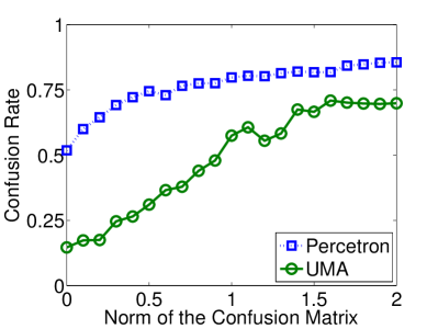
(a) Robustness to noise

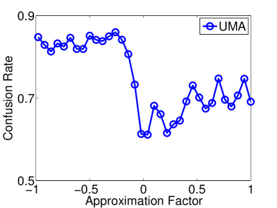
(b) Robustness to noise estimation

Figure 1: (a) evolution of the confusion rate (y-axis) for different noise levels (x-axis); (b) evolution of the same quantity with respect to errors in the confusion matrix $C$ (x-axis) measured by the approximation factor (see text).

On Figure 1(a) we observe that UMA clearly provides improvement over the Perceptron algorithm for every noise level tested, as it achieves lower confusion rates. Nonetheless, its performance degrades as the noise level increases, going from a confusion rate of $0.5$ for small noise levels—that is, when $\|{C-\texttt{diag}(C)}\|_{F}$ is small—to roughly $2.25$ when the noise is the strongest. Comparatively, the Perceptron algorithm follows the same trend, but with higher confusion rate, ranging from $1.7$ to $2.75$.

The second simulation (Fig. 1(b)) points out that, in addition to being robust to the noise process itself, UMA is also robust to underestimated (approximation factor $\rho>0$) noise levels, but not to overestimated (approximation factor $\rho<0$) noise levels. Unsurprisingly, the best confusion rate corresponds to an approximation factor of $0$, which means that UMA is using the true confusion matrix and can achieve a confusion rate as low as $1.8$. There is a clear gap between positive and negative approximation factors, the former yielding confusion rates around $2.6$ while the latter’s are slightly lower, around $2.15$. From these observations, it is clear that the approximation factor has a major influence on the performances of UMA.

4.2 Real data

4.2.1 Experimental Protocol

In addition to the results on synthetic data, we also perform simulations in a realistic learning scenario. In this section we are going to assume that labelling examples is very expensive and we implement the strategy evoked in Example 1. More precisely, for a given dataset $\mathcal{S}$, proceed as follows:

1. Ask for a small number $m$ of examples for each of the $Q$ classes.

2. Learn a rough classifier $g$ from these $Q\times m$ points.

3. Estimate the confusion $C$ of $g$ on a small labelled subset $\mathcal{S}_{\text{conf}}$ of $\mathcal{S}$.

4. Predict the missing labels $\bm{y}$ of $\mathcal{S}$ using $g$; thus, $\bm{y}$ is a sequence of noisy labels.

5. Learn the final classifier $f_{{\tt\normalsize U}{\tt MA}}$ from $\mathcal{S}$, $\bm{y}$, $C$ and measure its error rate.

One might wonder why we do not simply sample a very small portion of $\mathcal{S}$ in the first step. The reason is that in the case of very uneven classes proportions some of the classes may be missing in this first sampling. This is problematic when estimating $C$ as it leads to a non-invertible confusion matrix. Moreover, the purpose of $g$ is only to provide a baseline for the computation of $\bm{y}$, hence tweaking the class (im)balance in this step is not a problem.

In order to put our results into perspective, we compare them with results obtained from various algorithms. This allows us to give a precise idea of the benefits and limitations of UMA. Namely, we learn four additional classifiers: $f_{\bm{y}}$ is a regular Perceptron learned on $\mathcal{S}$ labelled with noisy labels $\bm{y}$, $f_{\text{conf}}$ and $f_{\text{full}}$ are trained with the correctly labelled training sets $\mathcal{S}_{\text{conf}}$ and $\mathcal{S}$ respectively and, lastly, $f_{\text{{\tt S3VM}}}$ is a classifier produced by a multiclass semi-supervised SVM algorithm (S3VM, Bennett ) run on $\mathcal{S}$ where only the labels of $\mathcal{S}_{\text{conf}}$ are provided. The performances achieved by $f_{\bm{y}}$ and $f_{\text{full}}$ provide bounds for UMA’s error rates: on the one hand, $f_{\bm{y}}$ corresponds to a worst-case situation, as we simply ignore the confusion matrix and use the regular Perceptron instead—arguably, UMA should perform better than this—; on the other hand, $f_{\text{full}}$ represents the best-case scenario for learning, when all the correct labels are available—the performance of $f_{\text{full}}$ should always top that of UMA (and the performances of other classifiers). The last two classifiers, $f_{\text{conf}}$ and $f_{\text{\text{{\tt S3VM}}}}$, provide us with objective comparison measures. They are learned from the same data as UMA but use them differently: $f_{\text{conf}}$ is learned from the reduced training set $\mathcal{S}_{\text{conf}}$ and $f_{\text{\text{{\tt S3VM}}}}$ is output by a semi-supervised learning strategy that infers both $f_{\text{\text{{\tt S3VM}}}}$ and the missing labels of $\mathcal{S}$ and it totally ignores the predictions $\bm{y}$ made by $g$. Note that according to the learning scenario we implement, we assume $C$ to be estimated from raw data. This might not always be the case with real-world problems and $C$ might be easier and/or less expensive to get than raw data; for instance, it might be deduced from expert knowledge on the studied domain. In that case, $f_{\text{conf}}$ and $f_{\text{\text{{\tt S3VM}}}}$ may suffer from not taking full advantage of the accurate information about the confusion.

4.2.2 Datasets

Our simulations are conducted on three different datasets. Each one with different features. For the sake of reproducibility, we used datasets that can be easily found on the UCI Machine learning repository Bache+Lichman:2013 . Moreover, these datasets correspond to tasks for which generating a complete, labelled, training set is typically costly because of the necessity of human supervision and subject to classification noise. The datasets used and their main features are as follows.

Optical Recognition of Handwritten Digits.

This well-known dataset is composed of $8\times 8$ grey-level images of handwritten digits, ranging from $0$ to $9$. The dataset is composed of $3,823$ images of $64$ features for training, and $1,797$ for the test phase. We set $m$ to $10$ for this dataset, which means that $g$ is learned from $100$ examples only. $\mathcal{S}_{\text{conf}}$ is a sampling of $5\%$ of $\mathcal{S}$. The classes are evenly distributed (see Figure 2(a)). We handle the nonlinearity through the use of a Gaussian kernel-PCA (see section 3.6) to project the data onto a feature space of dimension $640$.

Letter Recognition.

The Letter Recognition dataset is another well-known pattern recognition dataset. The images of the letters are summarized into a vector of $16$ attributes, which correspond to various primitives computed on the raw data. With $20,000$ examples, this dataset is much larger than the previous one. As for the Handwritten Digits dataset, the examples are evenly spread across the $26$ classes (see Figure 2(b)). We uniformly select $15,000$ examples for training and the remaining $5,000$ are used for test. We set $m$ to $50$ as it seems that smaller values do not yield usable confusion matrices. We again sample $5\%$ of the dataset to form $\mathcal{S}_{\text{conf}}$ and use, as before, a Gaussian kernel-based Kernel-PCA to (nonlinearly) expand the dimension of the data to $1,600$.

Reuters.

The Reuters dataset is a nearly linearly-separable document categorization dataset of more than $300,000$ instances of nearly $47,000$ features each. For size reasons we restrict ourselves to roughly $15,000$ examples for training, and $15,000$ other for test. It occurs that some classes are so underrepresented that they are flooded by the noise process and/or do not appear in $\mathcal{S}_{\text{conf}}$, which may lead to a non-invertible confusion matrix. We therefore restrict the dataset to the $9$ largest classes. One might wonder whether doing so erases class imbalance. This is not the case as, even this way, the least represented class accounts for roughly $500$ examples while this number reaches nearly $4,000$ for the most represented one (see Figure 2(c)). Actually, these $9$ classes represent more than $70$ percent of the dataset, reducing the training and test sets to approximately $11,000$ examples each. We do not use any kernel for this dataset, the data being already near to linearly-separable. Also, we sample $\mathcal{S}_{\text{conf}}$ on $5\%$ of the training set and we set $m=20$.

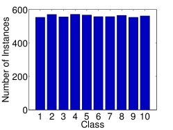
(a) Handwritten Digits

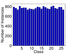
(b) Letter Recognition

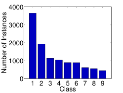
(c) Reuters

Figure 2: Class distribution for the three datasets.

4.2.3 Results

Table 1 presents the misclassification error rates averaged on $10$ runs. Keep in mind that we have not conducted a very thorough optimization of the hyper-parameters as the point here is essentially to compare UMA with the other algorithms. Additionally, we also report the error rates of $f_{\text{\text{{\tt S3VM}}}}$ when trained on the kernelized data with all dimensions, that is the kernelized data before we project them onto their $D$ principal components. Because the projection step is indeed unbecessary with S3VM, this will give us insights on the error due to the Kernel-PCA step. Comparing the first and the last columns of Table 1, it appears that UMA always induces a slight performance gain, i.e. a decrease of the misclassification rate, with respect to $f_{\bm{y}}$.

From the second and third columns of Table 1, it is clear that the reduced number of examples available to $f_{\text{conf}}$ induces a drastic increase in the misclassification rate with respect to $f_{\text{full}}$ which is allowed to use the totality of the dataset during the training phase.

Comparing UMA and $f_{\text{conf}}$ in Table 1 (fifth and second columns), we observe that UMA achieves lower misclassification rates on the Handwritten Digits and Letter Recognition datasets but a higher misclassification rate on Reuters. Although this is likely related to the strong class imbalance in the dataset. Indeed, some classes are overly represented, accounting for the vast majority of the whole dataset (see Fig. 2(c)). Because $\mathcal{S}_{\text{conf}}$ is uniformly sampled from the main dataset, $f_{\text{conf}}$ is trained with a lot of examples from the overrepresented classes and therefore it is very effective, in the sense that it achieves a low misclassification rate, for these overrepresented classes; this, in turn, induces a (global) low misclassification rate, as possibly high misclassification rates on underrepresented classes are countervailed by theirs accounting for a small portion of the data. On the other hand, because of this disparity in class representation, the slightest error in the confusion matrix, granted it involves one of these overrepresented classes, may lead to a significant increase of the misclassification rate. In this regard, UMA is strongly disadvantaged with respect to $f_{\text{conf}}$ on the Reuters dataset and it is the cause of the reported results.

The error rates for the S3VM and UMA classifiers are close for the Reuters and Handwritten Digits datasets whereas UMA has a clear advantage on the Letter Recognition problem. On the other hand, note that we used the S3VM method in conjunction with a Kernel-PCA for the sake of comparison with UMA in its kernelized form. The last column of Table 1 tends to confirm that this projection strategy increase the error rate of $f_{\text{\text{{\tt S3VM}}}}$. Also, reminds that the value of $m$ does not impact the performances of $f_{\text{\text{{\tt S3VM}}}}$ but has a significant effect on UMA, even though UMA never uses these labelled data. For instance, on the Reuters datasets, increasing $m$ from $20$ to $70$ reduces UMA’s error rate by nearly $0.1$ (see the error rates of Fig. 3 ($m=70$) when the size of labelled data is close to $550$, that is $5\%$ of the whole dataset). Despite our efforts to keep $m$ as small as possible, we could not go under $m=50$ for the Letter Recognition dataset without compromising the invertibility of the confusion matrix. The simple fact that an unusually high number of examples are required to simply learn a rough classifier asserts the complexity of this dataset. Moreover, the fact that $f_{\bm{y}}$ also outperforms $f_{\text{\text{{\tt S3VM}}}}$ implies that the labels fed to UMA are already mostly correct, and, according to our working assumptions, this is the most favorable setting for UMA.

Dataset	$f_{\bm{y}}$	$f_{\text{conf}}$	$f_{\text{full}}$	$f_{\text{\text{{\tt S3VM}}}}$	UMA	$f_{\text{\text{{\tt S3VM}}}}$ (no K-PCA)
Handwritten Digits	$0.25$	$0.21$	$0.04$	$0.15$	$0.16$	$0.07$
Letter Recognition	$0.35$	$0.36$	$0.23$	$0.49$	$0.33$	$0.18$
Reuters	$0.30$	$0.17$	$0.01$	$0.22$	$0.21$	$0.22$

Table 1: Misclassification rates of different algorithms.

Nonetheless, the disparities between UMA and $f_{\text{conf}}$ deserve more attention. Indeed, the same data are being used by both algorithms, and one could expect more closeness in the results. To get a better insight on what is occurring, we have reported the evolution of the error rate of these two algorithms with respect to the sampling size of $\mathcal{S}_{\text{conf}}$ in Figure 3. We can see that UMA is unaffected by the size of the sample, essentially ignoring the possible errors in the confusion matrix on small samples. This reinforces our previous results showing that UMA is robust to errors in the confusion matrix. On the other hand, with the addition of more samples, the refinement of the confusion matrix does not allow UMA to compete with the value of additional (correctly) labelled data and eventually, when the size of $\mathcal{S}_{\text{conf}}$ grows, $f_{\text{conf}}$ performs better than UMA. This points towards the idea that the aggregated nature of the confusion matrix incurs some loss of relevant information for the classification task at hand, and that a more accurate estimate of the confusion matrix, as induced by, e.g., the use of larger $\mathcal{S}_{\text{conf}}$, may not compensate for the information provided by additional raw data.

Building on this observation, we go a step further and replicate this experiment for all of the three datasets; only this time we track the performances of $f_{\text{\text{{\tt S3VM}}}}$ instead. The results are plotted on Figure 4. For the three datasets, we observe the same behavior as before. Namely, UMA is able to maintain a low error rate even with a very small size of $\mathcal{S}_{\text{conf}}$. On the other hand, UMA does not benefit as much as other methods from a large pool of labelled examples. In this case, UMA quickly stabilizes while, to the contrary, the S3VM method starts at a fairly high error rate and keeps improving as more labelled examples are available.

Beyond this, it is important to recall that UMA never uses the labels of $\mathcal{S}_{\text{conf}}$ (those are only used to estimate the confusion matrix, not the classifier—refer to Section 4.2.1 for the detailed learning protocol). While refining the estimation of $C$ is undoubtedly useful, a direction toward substantial performance gains should revolve around the combination of both this refined estimation of $C$ and the use of the correctly labelled training set $\mathcal{S}_{\text{conf}}$. This is a research subject on its own that we leave for future work.

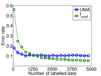
Figure 3: Error rate of UMA and $f_{\text{conf}}$ with respect to the sampling size. Reuters dataset with $m=70$ for the sake of figure’s readability.

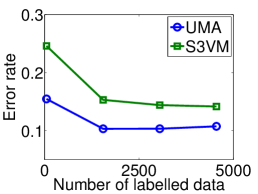
(a) Reuters dataset

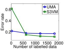
(b) Digits dataset

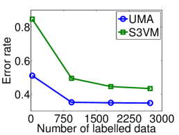
(c) Letter dataset

Figure 4: Error rates for the Reuter (left), optical digit recognition (center) and letter (right) datasets with respect to the size of $\mathcal{S}_{\text{conf}}$. Average over $15$ runs.

All in all, the reported results advise us to prefer UMA over other available methods when the amount of labelled data is particularly small, in addition, obviously, to the motivating case of the present work where the training data are corrupted and the confusion matrix is known. Also, another interesting finding we get is that even a rough estimation of the confusion matrix is sufficient for UMA to behave well.

Finally, we investigate the impact of the selection strategy of $(p,q)$ on the convergence speed of UMA (see Section 3.5). We use three variations of UMA with different strategies for selecting $(p,q)$ (error, confusion, and random) and monitor each one along the learning process on the Reuters dataset. The error and confusion strategies are described in Section 3.5 and the random strategy simply selects $p$ and $q$ at random.

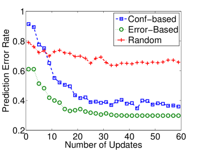
(a) Error rate

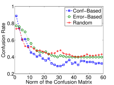
(b) Confusion rate

Figure 5: Error and confusion risk on Reuters dataset with various update strategies.

From Figure 5, which reports the misclassification rate and the confusion rate along the iterations, we observe that both performance measures evolve similarly, attaining a stable state around the $30$th iteration. The best strategy depends on the performance measure used, even though regardless of the performance measure used, we observe that the random selection strategy leads to a predictor that does not achieve the best performance measure (there is always a curve beneath that of the random selection procedure), which shows that it not an optimal selection strategy.

As one might expect, the confusion-based strategy performs better than the error-based strategy when the confusion rate is retained as a performance measure, while the converse holds when using the error rate. This observation motivates us to thoroughly study the confusion-based strategy in a near future as being able to propose methods robust to class imbalance is a particularly interesting challenge of multiclass classification.

The plateau reached around the $30$th iteration may be puzzling, since the studied dataset presents no positive margin and convergence is therefore not guaranteed. One possible explanation for this is to see the Reuters dataset as linearly separable problem corrupted by the effect of a noise process, which we call the intrinsic noise process that has structural features ‘compatible’ with the classification noise. By this, we mean that there must be features of the intrinsic noise such that, when additional classification noise is added, the resulting noise that characterizes the data is similar to a classification noise, or at least, to a noise that can be naturally handled by UMA. Finding out the family of noise processes that can be combined with the classification noise—or, more generally, the family of noise processes themselves—without hindering the effectiveness of UMA is one research direction that we aim to explore in a near future.

5 Conclusion

In this paper, we have proposed a new algorithm, UMA—for Unconfused Multiclass Additive algorithm—to cope with noisy training examples in multiclass linear problems. As its name indicates, it is a learning procedure that extends the (ultraconservative) additive multiclass algorithms proposed by crammer03ultraconservative ; to handle the noisy datasets, it only requires the information about the confusion matrix that characterizes the mislabelling process. This is, to the best of our knowledge, the first time the confusion matrix is used as a way to handle noisy label in multiclass problems.

One of the core ideas behind UMA, namely, the computation of the update vector $\bm{z}_{pq}$, is not tied to the additive update scheme. Thus, as long as the assumption of linear separability holds, the very same idea can be used to render a wide variety of algorithms robust to noise by iteratively generating a noise-free training set with the consecutive values of $\bm{z}_{pq}$. Although, every computation of a new $\bm{z}_{pq}$ requires learning a new classifier to start with. This may eventually incur prohibitive computational costs when applied to batch methods (as opposed to online methods) which are designed to process the entirety of the dataset at once. 

UMA takes advantage of the online scheme of additive algorithms and avoids this problem completely. Moreover, additive algorithms are designed to directly handle multiclass problem rather than having recourse to a bi-class mapping. The end-results of this are tightened theoretical guarantees and a convergence rate that does not depend of $Q$, the number of classes. Besides, UMA can be directly used with any additive algorithms, allowing to handle noise with multiple methods without further computational burden.

While we provide sample complexity analysis, it should be noted that a tighter bound can be derived with specific multiclass tools, such as the Natarajan’s dimension (see DanielySBS11 for example), which allow to better specify the expressiveness of a multiclass classifier. However, this is not the main focus of this paper and our results are based on simpler tools.

To complement this work, we want to investigate a way to properly tackle near-linear problems (such as Reuters). As for now the algorithm already does a very good jobs due to its noise robustness. However more work has to be done to derive a proper way to handle cases where a perfect classifier does not exist. We think there are great avenues for interesting research in this domain with an algorithm like UMA and we are curious to see how this present work may carry over to more general problems.

Acknowledgments.

The authors would like to thank the reviewers for their feedback and invaluable comments. This work is partially supported by the Agence Nationale de la Recherche (ANR), project GRETA 12-BS02-004-01. We would like to thank the anonymous reviewers for their insightful and extremely valuable feedback on earlier versions of this paper.

Appendix A Double sample theorem

Proof (Proposition 3)

For a fixed pair $(p,q)\in\mathcal{Y}^{2}$, we consider the family of functions

$$\mathcal{F}_{pq}\doteq\{f:f(\bm{x})\doteq\left<{\bm{w}_{q}-\bm{w}_{p}},{x}\right>:\bm{w}_{p},\bm{w}_{q}\in\mathcal{B}^{d}\}$$

where $\mathcal{B}^{d}$ is a $d$-dimensional unit ball. For each $f\in\mathcal{F}_{pq}$ define the corresponding “loss” function

$$l^{f}(\bm{x})\doteq l(f(\bm{x}))\doteq 2-f(\bm{x}).$$

Strictly speaking, $l^{f}(\bm{x})$ is not a loss as it does not take $y$ into account, nonetheless it does play the same role in the following proof than a regular loss in the regular double-sampling proof. One way to think of it is as the loss of a problem for which we do not care about the observed labels but instead we want to classify points into a predetermined class—in this case $q$.

Clearly, $\mathcal{F}_{pq}$ is a subspace of affine functions, thus $\text{Pdim}(\mathcal{F}_{pq})\leq(d+1)$, where $\text{Pdim}(\mathcal{F}_{pq})$ is the pseudo-dimension of $\mathcal{F}_{pq}$. Additionally, $l$ is Lipschitz in its first argument with a Lipschitz factor of $L\doteq 1$. Indeed $\forall y,y_{1},y_{2},\in\mathcal{Y}:|l(y_{1},y)-l(y_{2},y)|=|y_{1}-y_{2}|$.

Let $\mathcal{D}_{pq}$ be any distribution over $\mathcal{X}\times\mathcal{Y}$ and $T\in(\mathcal{X}\times\mathcal{Y})^{m}$ such that $T\sim\mathcal{D}_{pq}^{m}$, then define the empirical loss $\text{err}_{T}^{l}[f]\doteq\frac{1}{m}\sum_{\bm{x}_{i}\in T}l(\bm{x}_{i},y_{i})$ and the expected loss $\text{err}_{\mathcal{D}}^{l}[f]\doteq\mathbb{E}_{\mathcal{D}}\left[l(\bm{x},y)\right]$

The goal here is to prove that

$$\mathbb{P}_{T\sim\mathcal{D}_{pq}^{m}}\left(\sup_{f\in\mathcal{F}_{pq}}|\text{err}_{\mathcal{D}}^{l}[f]-\text{err}_{T}^{l}[f]|\geq\epsilon\right)\in\mathcal{O}\left(\left(\frac{8}{\epsilon}\right)^{(d+1)}e^{{m\epsilon^{2}}/_{128}}\right)$$ (21)

Proof (Proof of (21))

We start by noting that $l(y_{1},y_{2})\in[0,2]$ and then proceed with a classic $4$-step double sampling proof. Namely:

Symmetrization.

We introduce a ghost sample $T^{\prime}\in(\mathcal{X}\times\mathcal{Y})^{m}$, $T^{\prime}\sim\mathcal{D}_{pq}^{m}$ and show that for $f^{\text{bad}}_{T}$ such that $|\text{err}_{\mathcal{D}_{pq}}^{l}[f^{\text{bad}}_{T}]-\text{err}_{T}^{l}[f^{\text{bad}}_{T}]|\geq\epsilon$ then

$$\mathbb{P}_{T^{\prime}|T}\left(\left|\text{err}_{T^{\prime}}^{l}[f^{\text{bad}}_{T}]-\text{err}_{\mathcal{D}_{pq}}^{l}[f^{\text{bad}}_{T}]\right|\leq\frac{\epsilon}{2}\right)\geq\frac{1}{2},$$

as long as $m\epsilon^{2}\geq 32.$

It follows that

$$\mathbb{P}_{(T,T^{\prime})\sim\mathcal{D}_{pq}^{m}\times\mathcal{D}_{pq}^{m}}\left(\sup_{f\in\mathcal{F}_{pq}}|\text{err}_{T}^{l}[f]-\text{err}_{T^{\prime}}^{l}[f]|\geq\frac{\epsilon}{2}\right)$$

$$~{}\geq\mathbb{P}_{T\sim\mathcal{D}_{pq}^{m}}\left(|\text{err}_{T}^{l}[f^{\text{bad}}_{T}]-\text{err}_{\mathcal{D}_{pq}}^{l}[f^{\text{bad}}_{T}]|\geq\epsilon\right)\times\mathbb{P}_{T^{\prime}|T}\left(\left|\text{err}_{T^{\prime}}^{l}[f^{\text{bad}}_{T}]-\text{err}_{\mathcal{D}_{pq}}^{l}[f^{\text{bad}}_{T}]\right|\leq\frac{\epsilon}{2}\right)$$

$$~{}\geq\frac{1}{2}\mathbb{P}_{T\sim\mathcal{D}_{pq}^{m}}\left(|\text{err}_{T}^{l}[f^{\text{bad}}_{T}]-\text{err}_{\mathcal{D}_{pq}}^{l}[f^{\text{bad}}_{T}]|\geq\epsilon\right)$$

$$~{}=\frac{1}{2}\mathbb{P}_{T\sim\mathcal{D}_{pq}^{m}}\left(\sup_{f\in\mathcal{F}_{pq}}|\text{err}_{T}^{l}[f]-\text{err}_{\mathcal{D}_{pq}}^{l}[f]|\geq\epsilon\right) f^{\text{bad}}_{T}$$ (By definition of )

Thus upper bounding the desired probability by

$$2\times\mathbb{P}_{(T,T^{\prime})\sim\mathcal{D}_{pq}^{m}\times\mathcal{D}_{pq}^{m}}\left(\sup_{f\in\mathcal{F}_{pq}}|\text{err}_{T}^{l}[f]-\text{err}_{T^{\prime}}^{l}[f]|\geq\frac{\epsilon}{2}\right)$$ (22)

Swapping Permutations.

Let define $\Gamma_{m}$ the set of all permutations that swap one or more elements of $T$ with the corresponding element of $T^{\prime}$ (i.e. the $i$th element of $T$ is swapped with the $i$th element of $T^{\prime}$). It is quite immediate that $|\Gamma_{m}|=2^{m}$. For each permutation $\sigma\in\Gamma_{m}$ we note $\sigma(T)$ (resp. $\sigma(T^{\prime})$) the set originating from $T$ (resp. $T^{\prime}$) from which the elements have been swapped with $T^{\prime}$ (resp. $T$) according to $\sigma$.

Thanks to $\Gamma_{m}$ we will be able to provide an upper bound on (22). Our starting point is that $(T,T^{\prime})\sim\mathcal{D}_{pq}^{m}\times\mathcal{D}_{pq}^{m}$ then for any $\sigma\in\Gamma_{m}$, the random variable $\sup_{f\in\mathcal{F}_{pq}}|\text{err}_{T}^{l}[f]-\text{err}_{T^{\prime}}^{l}[f]|$ follows the same distribution as $\sup_{f\in\mathcal{F}_{pq}}|\text{err}_{\sigma(T)}^{l}[f]-\text{err}_{\sigma(T^{\prime})}^{l}[f]|$.

Therefore:

$$\mathbb{P}_{(T,T^{\prime})\sim\mathcal{D}_{pq}^{m}\times\mathcal{D}_{pq}^{m}}\left(\sup_{f\in\mathcal{F}_{pq}}|\text{err}_{T}^{l}[f]-\text{err}_{T^{\prime}}^{l}[f]|\geq\frac{\epsilon}{2}\right)$$

$$~{}=\frac{1}{2^{m}}\sum_{\sigma\in\Gamma_{m}}\mathbb{P}_{T,T^{\prime}\sim\mathcal{D}_{pq}^{m}\times\mathcal{D}_{pq}^{m}}\left(\sup_{f\in\mathcal{F}_{pq}}|\text{err}_{\sigma(T)}^{l}[f]-\text{err}_{\sigma(T^{\prime})}^{l}[f]|\geq\frac{\epsilon}{2}\right)$$

$$~{}=\mathbb{E}_{(T,T^{\prime})\sim\mathcal{D}_{pq}^{m}\times\mathcal{D}_{pq}^{m}}\left[\frac{1}{2m}\sum_{\sigma\in\Gamma_{m}}\mathbb{I}{\left\{\sup_{f\in\mathcal{F}_{pq}}|\text{err}_{\sigma(T)}^{l}[f]-\text{err}_{\sigma(T^{\prime})}^{l}[f]|\geq\frac{\epsilon}{2}\right\}}\right]$$

$$~{}\leq\sup_{(T,T^{\prime})\in(\mathcal{X}\times\mathcal{Y})^{2m}}\left[\mathbb{P}_{\sigma\in\Gamma_{m}}\left(\sup_{f\in\mathcal{F}_{pq}}|\text{err}_{\sigma(T)}^{l}[f]-\text{err}_{\sigma(T^{\prime})}^{l}[f]|\geq\frac{\epsilon}{2}\right)\right],$$ (23)

which concludes the second step.

Reduction to a finite class.

The idea is to reduce $\mathcal{F}_{pq}$ in (23) to a finite class of functions. For the sake of conciseness, we will not enter into the details of the theory of covering numbers. Please refer to the corresponding literature for further details (e.g. DevroyeGL ).

In the following, $\mathcal{N}({\epsilon}/_{8},\mathcal{F}_{pq},2m)$ will denote the uniform ${\epsilon}/_{8}$convering number of $\mathcal{F}_{pq}$ over a sample of size $2m$.

Let define $\mathcal{G}_{pq}\subset\mathcal{F}_{pq}$ such that $(l^{\mathcal{G}_{pq}})_{|(T,T^{\prime})}$ is an ${\epsilon/_{8}}$-cover of $(l^{\mathcal{F}_{pq}})_{|(T,T^{\prime})}$. Thus, $|\mathcal{G}_{pq}|\leq\mathcal{N}({\epsilon}/_{8},l^{\mathcal{F}_{pq}},2m)<\infty$ Therefore, if $\exists f\in\mathcal{F}_{pq}$ such that $|\text{err}_{\sigma(T)}^{l}[f]-\text{err}_{\sigma(T^{\prime})}^{l}[f]|\geq\frac{\epsilon}{2}$ then, $\exists g\in\mathcal{G}_{pq}$ such that $|\text{err}_{\sigma(T)}^{l}[g]-\text{err}_{\sigma(T^{\prime})}^{l}[g]|\geq\frac{\epsilon}{4}$ and the following comes naturally

$$\mathbb{P}_{\sigma\in\Gamma_{m}}\left(\sup_{f\in\mathcal{F}_{pq}}|\text{err}_{\sigma(T)}^{l}[f]-\text{err}_{\sigma(T^{\prime})}^{l}[f]|\geq\frac{\epsilon}{2}\right)$$

$$~{}\leq\mathbb{P}_{\sigma\in\Gamma_{m}}\left(\max_{g\in\mathcal{G}_{pq}}|\text{err}_{\sigma(T)}^{l}[g]-\text{err}_{\sigma(T^{\prime})}^{l}[g]|\geq\frac{\epsilon}{4}\right)$$

$$~{}\leq\mathcal{N}({\epsilon}/_{8},l^{\mathcal{F}_{pq}},2m)\max_{g\in\mathcal{G}_{pq}}\mathbb{P}_{\sigma\in\Gamma_{m}}\left(|\text{err}_{\sigma(T)}^{l}[g]-\text{err}_{\sigma(T^{\prime})}^{l}[g]|\geq\frac{\epsilon}{8}\right)$$ (union bound)

Hoeffding’s inequality.

Finally, consider $|\text{err}_{\sigma(T)}^{l}[g]-\text{err}_{\sigma(T^{\prime})}^{l}[g]|$ as the average of $m$ realizations of the same random variable, with expectation equal to $0$. Then by Hoeffding’s inequality we have that

$$\mathbb{P}_{\sigma\in\Gamma_{m}}\left(|\text{err}_{\sigma(T)}^{l}[g]-\text{err}_{\sigma(T^{\prime})}^{l}[g]|\geq\frac{\epsilon}{4}\right)\leq 2e^{{-m\epsilon^{2}}/_{128}}$$ (24)

Putting everything together yields the result w.r.t. $\mathcal{N}({\epsilon}/_{8},l^{\mathcal{F}_{pq}},2m)$ for $m\epsilon^{2}\geq 32$. For $m\epsilon^{2}<32$ it holds trivially.

Recall that $l^{\mathcal{F}_{pq}}$ is Lipschitz in its first argument with a Lipschitz constant $L=1$ thus $\mathcal{N}({\epsilon}/_{8},l^{\mathcal{F}_{pq}},2m)\leq\mathcal{N}({\epsilon}/_{8},\mathcal{F}_{pq},2m)=\mathcal{O}\left(\left(\frac{8}{\epsilon}\right)^{\text{Pdim}(\mathcal{F}_{pq})}\right)$

The last part of the proof comes from the observation that, for any fixed $(p,q)$, we had never used any other specific information about $\mathcal{F}_{pq}$ other than the upper bound of $d+1$ over its pseudo dimension. In other words, equation $\eqref{eq:result}$ holds for slightly modified definition of $\mathcal{F}_{pq}$ as long as the pseudo dimension does not exceed $d+1$.

Let us now consider :

$$\widehat{\mathcal{F}_{pq}}\doteq\{f:f(\bm{x})\doteq\mathbb{I}{\left\{t(\bm{x})=q\right\}}\mathbb{I}{\left\{\bm{x}\in\mathcal{A}_{p}^{\alpha}\right\}}\left<{\bm{w}_{p}-\bm{w}_{q}},{x}\right>:\bm{w}_{p},\bm{w}_{q}\in\mathcal{B}^{d}\}$$

Clearly for each function in $\widehat{\mathcal{F}_{pq}}$ there is at most one corresponding affine function, thus $\widehat{\mathcal{F}_{pq}}$ and $\mathcal{F}_{pq}$ share the same upper bound of $d+1$ on their pseudo-dimension.

Consequently, any covering number of $\mathcal{F}_{pq}$ is also a covering number of $\widehat{\mathcal{F}_{pq}}$. More precisely, this proof holds true for any $\bm{w}_{p}$ and $\bm{w}_{q}$, independently of $\mathcal{A}_{p}^{\alpha}$ which may itself be defined with respect to $\bm{w}_{p}$ and $\bm{w}_{q}$.

It comes naturally that, fixing $S$ as the training set, the following holds true:

$$\frac{1}{m}\sum_{m}\mathbb{I}{\left\{t(\bm{x})=q\right\}}\mathbb{I}{\left\{\bm{x}\in\mathcal{A}_{p}^{\alpha}\right\}}\bm{x}=\bm{z}_{pq}.$$

Thus

$$\left|\text{err}_{T}^{l}[f]-\text{err}_{D}^{l}[f]\right|=\left|\left<{\frac{\bm{w}_{p}-\bm{w}_{q}}{\|{\bm{w}_{p}-\bm{w}_{q}}\|}},{\bm{z}_{pq}}\right>-\left<{\frac{\bm{w}_{p}-\bm{w}_{q}}{\|{\bm{w}_{p}-\bm{w}_{q}}\|}},{\mu_{p}^{q}}\right>\right|.$$

We can generalize this result for any couple $(p,q)$ by a simple union bound, giving the desired inequality:

$$\mathbb{P}_{(\mathcal{X}\times\mathcal{Y})\sim\mathcal{D}} \left(\sup_{W\in\mathbb{R}^{d\times Q}}\left|\left<{\frac{\bm{w}_{p}-\bm{w}_{q}}{\|{\bm{w}_{p}-\bm{w}_{q}}\|}},{\bm{z}_{pq}}\right>-\left<{\frac{\bm{w}_{p}-\bm{w}_{q}}{\|{\bm{w}_{p}-\bm{w}_{q}}\|}},{\mu_{p}^{q}}\right>\right|\geq\epsilon\right)$$

$$\qquad\leq\mathcal{O}\left(Q^{2}\left(\frac{8}{\epsilon}\right)^{(n+1)}e^{{m\epsilon^{2}}/_{128}}\right)$$

Equivalently, we have that

$$\left|\left<{\frac{\bm{w}_{p}-\bm{w}_{q}}{\|{\bm{w}_{p}-\bm{w}_{q}}\|}},{\bm{z}_{pq}}\right>-\left<{\frac{\bm{w}_{p}-\bm{w}_{q}}{\|{\bm{w}_{p}-\bm{w}_{q}}\|}},{\mu_{p}^{q}}\right>\right|\geq\epsilon$$

with probability $1-\delta$ for

$$m\in\mathcal{O}\left(\frac{1}{\epsilon^{2}}\left[\ln\left(\frac{1}{\delta}\right)+\ln(Q)+d\ln\left(\frac{1}{\epsilon}\right)\right]\right).$$

References

- (1) Bach, F.R., Jordan, M.I.: Kernel Independent Component Analysis. Journal of Machine Learning Research 3, 1–48 (2002)
- (2) Bache, K., Lichman, M.: UCI machine learning repository (2013). URL http://archive.ics.uci.edu/ml
- (3) Bennett, K.P., Demiriz, A.: Semi-supervised support vector machines. In: Advances in Neural Information Processing Systems, pp. 368–374. MIT Press (1998)
- (4) Blanchard, G., Zwald, L.: Finite-dimensional projection for classification and statistical learning. IEEE Transactions on Information Theory 54(9), 4169–4182 (2008)
- (5) Block, H.: The perceptron: a model for brain functioning. Reviews of Modern Physics 34, 123–135 (1962)
- (6) Blum, A., Frieze, A.M., Kannan, R., Vempala, S.: A Polynomial-Time Algorithm for Learning Noisy Linear Threshold Functions. In: Proc. of 37th IEEE Symposium on Foundations of Computer Science, pp. 330–338 (1996)
- (7) Bylander, T.: Learning Linear Threshold Functions in the Presence of Classification Noise. In: Proc. of 7th Annual Workshop on Computational Learning Theory, pp. 340–347. ACM Press, New York, NY, 1994 (1994)
- (8) Cohen, E.: Learning Noisy Perceptrons by a Perceptron in Polynomial Time. In: Proc. of 38th IEEE Symposium on Foundations of Computer Science, pp. 514–523 (1997)
- (9) Crammer, K., Dekel, O., Keshet, J., Shalev-Shwartz, S., Singer, Y.: Online passive-aggressive algorithms. JMLR 7, 551–585 (2006)
- (10) Crammer, K., Singer, Y.: Ultraconservative online algorithms for multiclass problems. Journal of Machine Learning Research 3, 951–991 (2003)
- (11) Cristianini, N., Shawe-Taylor, J.: An Introduction to Support Vector Machines and other Kernel-Based Learning Methods. Cambridge University Press (2000)
- (12) Daniely, A., Sabato, S., Ben-David, S., Shalev-Shwartz, S.: Multiclass learnability and the ERM principle. Journal of Machine Learning Research - Proceedings Track 19, 207–232 (2011)
- (13) Dekel, O., Shalev-shwartz, S., Singer, Y.: The forgetron: A kernel-based perceptron on a fixed budget. In: In Advances in Neural Information Processing Systems 18, pp. 259–266. MIT Press (2005)
- (14) Devroye, L., Györfi, L., Lugosi, G.: A Probabilistic Theory of Pattern Recognition. Springer (1996)
- (15) Drineas, P., Kannan, R., Mahoney, M.W.: Fast Monte Carlo algorithms for matrices ii: computing a low rank approximation to a matrix. SIAM Journal on Computing 36(1), 158–183 (2006)
- (16) Drineas, P., Mahoney, M.W.: On the Nyström method for approximating a gram matrix for improved kernel-based learning. Journal of Machine Learning Research 6(Dec), 2153–2175 (2005)
- (17) Freund, Y., Schapire, R.E.: Large Margin Classification Using the Perceptron Algorithm. Machine Learning 37(3), 277–296 (1999)
- (18) Friess, T., Cristianini, N., Campbell, N.: The Kernel-Adatron Algorithm: a Fast and Simple Learning Procedure for Support Vector Machines. In: J. Shavlik (ed.) Machine Learning: Proc. of the Int. Conf. Morgan Kaufmann Publishers (1998)
- (19) Kakade, S.M., Shalev-Shwartz, S., Tewari, A.: Efficient bandit algorithms for online multiclass prediction. In: Proceedings of the 25th International Conference on Machine Learning, ICML ’08, pp. 440–447. ACM, New York, NY, USA (2008)
- (20) Kearns, M.J., Vazirani, U.V.: An Introduction to Computational Learning Theory. MIT Press (1994)
- (21) Louche, U., Ralaivola, L.: Unconfused ultraconservative multiclass algorithms. In: JMLR Workshop & Conference Proc. 29, (Proc. of ACML 13), pp. 309–324 (2013)
- (22) Minsky, M., Papert, S.: Perceptrons: an Introduction to Computational Geometry. MIT Press (1969)
- (23) Novikoff, A.: On convergence proofs for perceptrons. In: Proc. of the Symposium on the Mathematical Theory of Automata, Vol. 12, pp. 615–622 (1963)
- (24) Ralaivola, L.: Confusion-based online learning and a passive-aggressive scheme. In: NIPS, pp. 3293–3301 (2012)
- (25) Ralaivola, L., Favre, B., Gotab, P., Bechet, F., Damnati, G.: Applying multiclass bandit algorithms to call-type classification. In: ASRU, pp. 431–436 (2011)
- (26) Schölkopf, B., Smola, A.J.: Learning with Kernels, Support Vector Machines, Regularization, Optimization and Beyond. MIT University Press (2002). URL http://www.learning-with-kernels.org
- (27) Stempfel, G., Ralaivola, L.: Learning kernel perceptron on noisy data and random projections. In: In Proc. of Algorithmic Learning Theory (ALT 07) (2007)
- (28) Takerkart, S., Ralaivola, L.: MKPM: a multiclass extension to the kernel projection machine. In: CVPR, pp. 2785–2791 (2011). URL http://dblp.uni-trier.de/db/conf/cvpr/cvpr2011.html#TakerkartR11
- (29) Valiant, L.: A theory of the learnable. Communications of the ACM 27, 1134–1142 (1984)
- (30) Williams, C.K.I., Seeger, M.: Using the Nyström Method to Speed Up Kernel Machines. In: Advances in Neural Information Processing Systems 13, pp. 682–688. MIT Press (2001)