Incremental RANSAC for Online Relocation in Large Dynamic Environments
Abstract
Vehicle relocation is the problem in which a mobile robot has to estimate the self-position with respect to an a priori map of landmarks using the perception and the motion measurements without using any knowledge of the initial self-position. Recently, RANdom SAmple Consensus (RANSAC), a robust multi-hypothesis estimator, has been successfully applied to offline relocation in static environments. On the other hand, online relocation in dynamic environments is still a difficult problem, for available computation time is always limited, and for measurement include many outliers. To realize real time algorithm for such an online process, we have developed an incremental version of RANSAC algorithm by extending an efficient preemption RANSAC scheme. This novel scheme named incremental RANSAC is able to find inlier hypotheses of self-positions out of large number of outlier hypotheses contaminated by outlier measurements.
I Introduction
For safe and efficient navigation, it is crucial for a mobile robot to estimate the self-position with respect to an a priori given map of point landmarks called global map using the perception and the motion measurements without using any knowledge of the initial self-position. This problem is called vehicle relocation (also ”global localization”, or ”kidnapped robot problem”), and has received considerable attention over the last decades [1][2]. A relocation problem can be classified into offline or online, according to whether the localization takes place after or during the robot navigation. Especially, online relocation is more challenging due to the limitation on the available computation time. Previous studies on online relocation have focused on static environments [1][3] or small environments [4][5], and little study has been done on relocation scalable to large dynamic environments.
RANdom SAmple Consensus (RANSAC) [6] is one of most effective algorithms that have been successfully applied to offline relocation in large-scale static environments [2][7]. In the context of relocation, RANSAC acts as a robust map-matching algorithm, estimating the self-position by matching between the global map of landmarks and a local map of observed features. The algorithm randomly generates a set of self-position hypotheses by matching minimal sets of features and landmarks, and then scores each hypothesis by counting the number of other matches. Despite its simplicity, RANSAC performs very well in the presence of outlier features. In the famous study carried out by Neira, Tards and Castellanos [2], the effectiveness of RANSAC-based relocation over conventional algorithms was demonstrated. However, the original RANSAC is essentially offline algorithm and is not directly applicable to the online relocation, where features incrementally arrive and available time is always limited. Moreover, its computational complexity depends strongly on the number of features and outliers.
This paper focuses on the problem of RANSAC-based online relocation in large-scale dynamic environments. In such an online process, the robot can no longer score all the hypotheses by the full set of features due to the limitation on the computation time, instead it can only score a small set of hypotheses by a small set of features. So, the robot is required to plan the order in which hypotheses and features are scored, so as to avoid excessive scoring of useless hypotheses or features, which are contaminated by outliers inherent in large or dynamic environments. To solve this problem, we propose to utilize an efficient RANSAC scheme, called preemption scheme, which was originally proposed for computer vision applications by Nister [8]. The only difference of this preemptive RANSAC from the standard one is that the scoring order is planned to achieve high efficiency in the limited time. Importantly, this technique puts no constraint on the hypothesis generation, e.g. avoiding any guided hypothesis generation. We have developed an incremental version of the preemptive RANSAC, named incremental RANSAC, which can handle incrementally arriving features while requiring a constant time per viewpoint. We apply this novel RANSAC scheme for matching the global map and a local map that is incrementally updated in a constant time by utilizing Sparse Extended Information Filter (SEIF). As a result, our real-time algorithm worked robustly in large dynamic environments even where more than of the landmarks have been modified.
II Related Works
Previous techniques for online localization can be classified into two categories, according to whether the initial self-position is known or not. If the initial self-position is known, the localization problem is equivalent to position tracking, and traditional techniques such as Kalman Filtering [5][9] are applicable. If the initial self-position is unknown, the full relocation problem needs to be solved.
Markov Localization and Monte Carlo Localization [1] are two popular algorithms for online relocation. They generate a number of self-position hypotheses covering all possible positions and score the likelihood of every hypothesis based on consistency between features and landmarks. Although they are reliable in relatively small environments [3], they are not scalable to large environments since the number of required hypotheses is linear to the environment size.
There are also some offline algorithms that are scalable to large environments. They aim to estimate the self-position by matching between the global landmark map and a local feature map. The essence of these algorithms is to generate a small set of good initial hypotheses by matching minimal set of features and landmarks [2][7]. As briefly described in section I, RANSAC is one of such algorithms. Their computational cost depends not on the environment size but on the number of features, therefore they are efficient especially in sparse environments [3]. However, even these algorithms are not directly applicable to online relocation, where available computation time is always limited and typically constant. Moreover, larger number of features would be required in the case of dynamic environments since there are usually many outlier features. This makes it difficult even to apply some pre-computed lookup tables that could accelerate the map matching [4].
III Background
III-A Problem
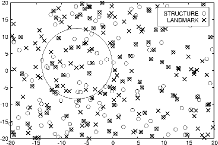
The goal of relocation is to estimate the self-position of the robot with respect to a priori given map by using motion and perception sensors without using any a priori knowledge of the initial self-position. Online relocation is a process to incrementally update the belief of the self-position every time new motion and perception measurements arrive. Following the SLAM literature [10], the a priori map is called global map and represented by a set of 2D point landmarks. Each landmark is a cartesian pair. There is no distinctive landmark that is distinguishable from another landmark. The motion sensor acquires the ego-motion of the robot on the floor plane. The perception sensor acquires relative position to the surrounding landmarks. A popular example of the motion and the perception sensors is omni- laser scanner and wheel encoder. Fig. 1 shows the area observed by the perception sensor at a certain viewpoint as a circular region.
Features observed at more than one viewpoint are often required to uniquely determine the self-position. In such a case, it is useful to construct a local map of features from scratch through a SLAM process during the robot navigation. When the local map grows sufficiently informative, the self-position will be uniquely determined by matching the global and the local maps.
We will utilize SEIF [11], a constant time SLAM filter, to update the local map as well as the self-position with respect to the local map. Instead of traditional representation in Kalman Filter using a mean vector and a covariance matrix, SEIF represents the current estimate of the system state (i.e. self-position and map) by so-called information matrix and information vector. Information matrix is the inverse of the covariance matrix, and naturally sparse i.e. it tends to have much less strong constraints than the covariance matrix. In SEIF, the sparseness of the information matrix is enhanced by a process called sparsification that eliminates weak robot-landmark constraints. As a result, the perception and the motion update can be done in a constant time. The local map can be also recovered from the information matrix and the information vector in a constant time by a process called amortized map recovery. For more details of SEIF, see [11].
In large dynamic environments, there are mainly two sources of outlier features. First, the robot is not necessarily located in the mapped area, the area covered by the global map. In addition, the robot does not know whether it is located in mapped or unmapped area. Therefore, while it navigates in unmapped area, it obtains only outlier measurements. Second, some landmarks may have been modified due to environment changes. Fig. 1 illustrates an example of such environment changes. In this figure, ’STRUCTURE’ and ’LANDMARK’ points respectively indicate landmark locations after and before the environment changes. Landmarks can be removed, added or even moved from one place to another. Such dummy (changed) landmarks tend to increase outlier measurements. Moreover, removed landmarks will cause even reduction of inlier measurements. Therefore, we view this second outlier source is more critical. All of above mentioned outliers are not simply distinguishable from inliers.
III-B Probabilistic Formulation
The relocation problem is formulated in a probabilistic framework. In the following, we denote by a sequence . Let denote the a priori given global map. denote measurement arrives at time . can be a motion or perception measurement. Without loss of generality, we assume each perception measurement corresponds to exactly one landmark in the environment. Let denote the set of parameters estimated by SEIF, i.e. the local map and the self-position with respect to the local map. Since the global map and the local map are represented in different coordinate systems, the coordinate transformation (rotation and translation) from the local map to the global map also needs to be estimated. Let denote such a transformation, which we call global position. Then, the system state to estimate is represented by . Based on the above terminology, the online relocation is formulated as the problem of incrementally updating the belief from to every time new measurement arrives. This probability density can be decomposed in the form
| (1) |
then both the terms and can be efficiently updated in the following manner. The first term is the probability density that can be estimated from in a constant time by SEIF as discussed in section III-A. The second term can be approximated by , since can be viewed as a summary of the history of observations. We view the problem of estimating as a kind of map matching problems, to search a best transformation by which the local map in and the global map maximally overlap.
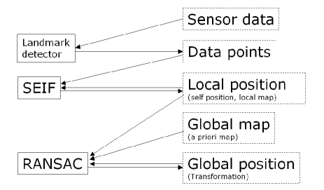
(a) System architecture.

(b) Estimation by SEIF.
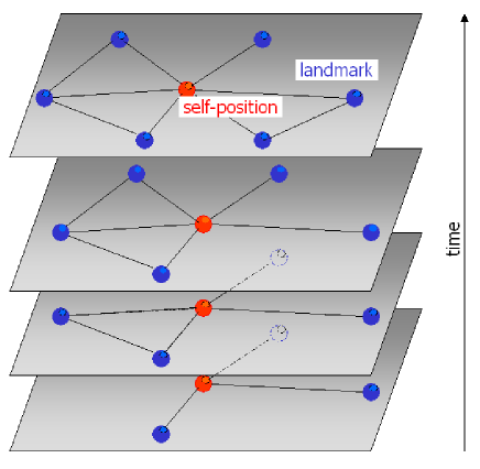
(c) Gradually changing map.
III-C System Overview
Fig. 2(a) illustrates the system architecture. The landmark detector tracks and detects moving objects based on relative speed of surrounding objects, and then outputs features that are likely to correspond to static landmarks. Using such output features as well as the motion measurements, the SEIF filter updates the probability density from to . Fig. 2(b) illustrates an example of features (’+’) estimated by SEIF, as well as the true robot trajectory (’’) and the true landmark locations (’’). RANSAC module updates the belief of the global position by matching the global map and the local map. Note that this matching problem gradually changes over time as the local map is incrementally updated. As shown in the simple example in Fig. 2(c), the local map is updated every time new features arrive or old features are updated by SEIF. We will present a constant-time RANSAC algorithm suitable for such incrementally changing matching problems in section IV.
IV Incremental RANSAC
IV-A RANSAC-based Map-matching
RANSAC is a robust multi-hypothesis estimator in the presence of many outlier features. In the context of relocation, a feature corresponds to one feature in the local map while a hypothesis corresponds to one hypothesis of global position , a transformation from the local to the global coordinate. RANSAC is essentially an offline algorithm, for it assumes all the features are a priori given.
The algorithm is summarized as follows. In the initialization stage, the system randomly permutes the features. Then, it iterates the following steps until the time budget is exhausted.
-
1.
Generate a hypothesis from randomly selected features by matching the features with landmarks.
-
2.
Initialize score of the hypotheses to .
-
3.
For each feature , check if is an inlier pair, and if so increment . Here, is judged as inlier iff the feature transformed to the global coordinate by is located within a neighborhood of some landmark.
When the process finishes, a hypothesis with highest score is output as the best transformation . Usually, the computational cost of the step 1 or 2 is negligible compared to the cost of step 3, therefore the total cost is approximately linear to the number of feature-hypothesis pairs.
The parameter should be carefully determined taking into account the tradeoff between efficiency and reliability. In step 1, at least two features are required to uniquely determine a hypothesis i.e. the global position , therefore . As increases, the easier it is to reduce outlier hypotheses by using the () redundant features, therefore it becomes easier to increase the efficiency. On the other hand, as decreases, the higher the probability of at least one hypothesis being inlier, therefore the reliability increases. We set , and randomly select such features that are covisible from at least one viewpoint. This is similar in concept with the ’locality’ suggested in [2]. We found that this procedure generates almost constant number of new hypotheses every time a new feature arrives.
IV-B Preemptive RANSAC
Even with the above procedure, the number of hypotheses is linear to the number of observations. Fig. 3 shows how the number of features and hypotheses grows as the robot navigates. Obviously, it is difficult for the original RANSAC to achieve constant-time online relocation.
It can be viewed that the original RANSAC scores all the feature-hypothesis pairs excessively. Although such an algorithm is reliable, its computational cost is at least the square order of the number of observations. Instead of such an excessive scoring, the preemption scheme proposed by Nister [8] plans scoring order in which pairs are scored so as to avoid scoring useless pairs. In the following, we briefly summarize the scheme.
A preemption scheme is composed of an order rule and a preference rule :
| (2) |
An order rule determines the next pair to be scored given all the previous scoring results:
| (3) |
Here, represents the score of the hypothesis . A preference rule selects the most preferred (best) hypothesis given all the scoring results:
| (4) |
A preemption scheme is called depth-first if the order obeys
| (5) |
or called breadth-first if the order obeys
| (6) |
or called hybrid otherwise. In the next section, this efficient offline scheme will be extended for our online relocation problem.

IV-C Incremental Scheme
To deal with incrementally arriving features, we have developed a novel RANSAC scheme, named incremental RANSAC, which combines the advantages of the RANSAC-based map-macthing (section IV-A) and the preemptive RANSAC (section IV-B). This novel scheme has the following two characteristics:
-
1.
Incremental estimation: at every viewpoint, feature-hypothesis pairs are scored conditioned on the scoring results at the previous viewpoints.
-
2.
Real-time estimation: at every viewpoint, only a constant number of feature-hypothesis pairs are selected to be scored within the limited computation time.
The incremental scheme is summarized as follows. For incremental estimation, the scheme maintains two kinds of lists called feature list and hypothesis list , which respectively record already arrived but not yet scored features and hypotheses. In the initialization stage at , the robot sets the lists , to null. At every viewpoint, firstly, the robot updates the lists and in the following steps, which is essential to realize the incremental estimation.
-
1-1)
Add newly arrived features to , then randomly permute .
-
1-2)
Generate new hypotheses . Here, each hypothesis should be generated from randomly selected features, at least one of which is a newly arrived feature.
-
1-3)
Add to , then randomly permute .
Secondly, the robot iterates the following steps for times, which is essential to realize the real-time estimation.
-
2-1)
Determine the next pair by the order rule.
-
2-2)
If is an inlier pair, increment .
-
2-3)
If is a member of , then eliminate from .
-
2-4)
If is a member of , then eliminate from .
Fig. 4 (a) and (b) respectively show examples of the orders determined by the depth-first and the breadth-first order rules in the incremental RANSAC scheme. As can be seen from the figures, incremental RANSAC is essentially a hybrid scheme.
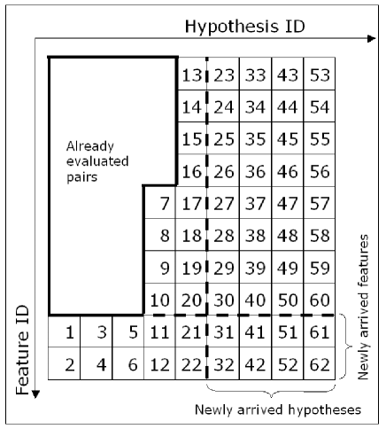
(a) Depth-first order rule.
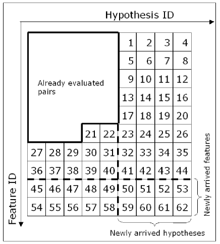
(b) Breadth-first order rule.
Generally, there is no reason to score a pair twice. Some simple order rules, including the depth-first and the breadth-first rules, may perfectly avoid such loss. However, more complex order rules can avoid such loss only by memorizing all of the already-scored pairs. Unfortunately, this requires memory space proportional to the square of the number of observations. To solve this problem, our method clears the memory every time the robot reaches a new viewpoint. Although this does not guarantee that no loss will occur, this requires only constant size memory space.
IV-D Preference Rule
The most popular preference rule for the original RANSAC is to select a hypothesis with the highest score. However, in our case, the score does not directly reflect the likelihood of a hypothesis being inlier, since the probability of scoring each hypothesis is not equal. We found that the above preference rule is often unreliable in the case of incremental RANSAC. To deal with the problem, the preference rule must be given in a normalized form:
| (7) | |||||
| (8) |
Here, is the total number of the hypothesis being scored. So, represents the ratio of the hypothesis being scored as inlier.
IV-E Order Rule
Both of the depth-first and the breadth-first schemes have some appealing properties.
-
•
A depth-first scheme tends to score small set of hypotheses by full set of features. Most of existing techniques for RANSAC-based relocation [2][7] can be classified into depth-first scheme. Joint Compatibility Test [12] is a technique to accurately discriminate between similar hypotheses using many features.
-
•
A breadth-first scheme tends to score full set of hypotheses by a small set of features. A breadth-first scheme has been successfully applied to a practical real-time application of Structure From Motion (SFM) [8] where many hypotheses are contaminated by outlier features.
Cleary, they also have some limitations.
-
•
The depth-first scheme is effective only if the ratio of inlier hypotheses is sufficiently high [6].
-
•
The breadth-first scheme is effective only if relatively small number of features are required to distinguish inlier hypotheses from outlier ones [8].
Unfortunately, these are not the case in our problem. In large and dynamic environments, the ratio of inlier hypotheses is low, and many hypotheses are not easily distinguishable.
To solve the problems, we propose to use some hybrid order rule which is based on the following criteria.
-
1.
Diversification: score as many hypotheses as possible.
-
2.
Intensification: score preferred hypotheses by using as many features as possible.
The criteria 1) and 2) are respectively similar in concept with the breadth-first and the depth-first schemes. In general, there is a tradeoff between the diversification and the intensification of an optimization algorithm.
To implement the above idea, our algorithm classifies all the hypotheses into several groups
| (9) |
of different preference levels according to the previous scoring results. Let denote the number of hypotheses belonging to group #i. Our classification rule is to determine the group ID by
| (10) |
The larger ID means higher preference level. Based on the classification results, the algorithm randomly selects
| (11) |
hypotheses in total from each group . Here, is a weighting function called preemption function, which prioritizes different groups based on their relative importance. is a normalizing coefficient that makes
| (12) |
For each selected hypothesis, the algorithm generates a pair composed of the hypothesis and a randomly selected feature. In this way, it generates pairs in total, which our order rule will output one by one.
We use a simple preemption function in the form:
| (13) |
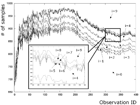
In experiments described in section V, we simply set . This means that the probability of a hypothesis in a group being scored is almost twice the probability of a hypothesis in the group being scored. Also, we will use , which means that ranges from to .
Fig. 5 shows an example of the number of hypotheses selected from each group for . In this example, the number is largest for group #0 due to large group size , and next largest for group #9 due to high weight . Note that these two results respectively correspond to the two criteria, diversification and intensification, described above.
To determine the next pair, our algorithm determines the hypothesis before it randomly selects the feature. Note that once it determines the hypothesis i.e. the transformation , it can uniquely determine the location of any (already-arrived) feature with respect to the global map. Therefore, there is no reason to select a feature located in an unmapped area. Our algorithm can avoid selecting such useless features by selecting the feature in the following steps.
-
1.
Randomly sample a location in the mapped areas.
-
2.
Output such a feature that is nearest to .
The search process in the second step can be executed quite fast based on a space division technique using quadtree. Such a selection strategy must be important especially when the ratio of outlier features becomes large.
V Experimental Evaluation
To evaluate the robustness of the proposed method against outlier observations, we conducted a number of experiments in virtual environments. The robot is equipped with an omni- laser scanner that can observe landmarks within , with Gaussian noise with standard deviation in range and in azimuth. The robot is also equipped with a wheel encoder that measures translation and rotation movement with Gaussian noise with standard deviation. Fig. 6 shows an example of the environments. The environment size is . The robot is initially located at , and moves towards the goal location at . Every time it moves , it observes the surroundings by the laser scanner. Based on the latest measurements, it updates its belief by the SEIF as well as the incremental RANSAC.
Every virtual environment is generated in the following manner. Mapped area is , only of the entire environment. landmarks are randomly distributed in the environment. A predetermined ratio (ranging from to as described later) of landmarks have been moved due to environment changes. Such high landmark density, small mapped area, as well as environment changes cause many outlier features and hypotheses, which make our relocation problem more difficult.
To evaluate the performance for various outlier ratio, we generated test environments of different ratio of changes, ranging from to . We tested the proposed method and benchmark against two other methods, a depth-first method and a breadth-first method described in IV. To achieve real-time processing, had to be set to a small number, . The computational costs of our relocation process per viewpoint (CPU Pentium4 , ) are as follows.
-
•
SEIF:
-
–
perception update:
-
–
motion update:
-
–
amortized map recovery:
-
–
the others (including the sparsification):
-
–
-
•
RANSAC: ()
The total computational cost is less than , which is sufficiently low cost for many real-time applications [10].
Fig. 7 summarizes the results. The horizontal axis indicates the ratio of changed landmarks, while the vertical axis indicates the localization error at the (estimated) goal location.


The depth-first scheme was successful when the order rule selects at least one inlier hypothesis. However, the probability of selecting such an inlier hypothesis in the limited computation time is inverse proportion to the number of the pairs. As a result, the method became unreliable if the change ratio exceeds .
The breadth-first scheme gives the maximum probability of scoring inlier hypotheses over all possible preemption schemes. However, the method could not score inlier hypotheses by many features due to the limitation on the computation time.
On the other hand, our hybrid scheme performed very well. Especially, when the change ratio is less than , the method achieved low localization error, less than . Like the breadth-first scheme, the method gives a high probability of scoring inlier hypotheses. Also, like the depth-first scheme, the method scores preferred hypotheses (i.e. hypotheses in high preference groups) by many features. From the results, it can be concluded that the proposed incremental RANSAC gives a scheme of a real-time process for robust online relocation in large and dynamic environments.
VI Conclusions & Future Works
In this paper, the problem of online relocation in large dynamic environments was addressed. To make the problem computationally tractable, the problem was decomposed into a problem of local map updating, and a problem of map matching. The map matching problem gradually changes over time due to the local map updating as well as incrementally arriving features. To deal with the problem, an efficient RANSAC scheme called preemptive RANSAC was modified, and an incremental version named incremental RANSAC was proposed. The robustness of the proposed algorithm against outlier observations was demonstrated in a number of large and dynamic environments.
In the future, we will develop our research along two lines. First, we plan to implement and evaluate the proposed algorithm on a real mobile robot. In complex and less sparse environments, transformation of real range data to feature may be itself a difficult problem. Some grid-based representation [13][14] of the map instead of the feature-based representation chosen in this paper, may be effective to deal with such ambiguity. In addition, the landmark detection problem described in section III-C, which was simplified in this paper, will become more challenging task. Second, we plan to study a way to extend the proposed relocation techniques for SLAM problems, where the landmarks should be learned even in large and dynamic environments.
Acknowledgment
This research was partially supported by the Japan Ministry of Education, Science, Sports and Culture, Grant in-Aid for Young Scientists (B), 17700200, 2005.
References
- [1] Thrun S., Fox D., Burgard W., and Dellaert F. Robust monte carlo localization for mobile robots. Artificial Intelligence Journal, 2001.
- [2] Jos Neira, Juan D. Tards, and A. Castellanos. Linear time vehicle relocation in slam. Proc. 2003 IEEE Int. Conf. Robotics and Automation, pages 427–433, 2003.
- [3] Lina M. Paz, Pdro Pinis, Jos Neira, and Juan D. Tards. Global localization in slam in bilinear time. Proc. 2005 IEEE/RSJ Int. Conf. Intelligent Robots and Systems, pages 655–661, 2005.
- [4] Fox D., Burgard W., and Thrun S. Markov localization for mobile robots in dynamic environments. Artificial Intelligence Research, 11:391–427, 1999.
- [5] Denis Wolf and Gaurav S. Sukhatme. Online Simultaneous Localization and Mapping in Dynamic Environments. IEEE Int. Conf. Robotics and Automation, pages 1301–1307, 2004.
- [6] Martin A. Fischler and Robert C. Bolles. Random sample consensus: A paradigm for model fitting with apphcatlons to image analysis and automated cartography. Communications of the ACM, 24(6):381–395, 1981.
- [7] David C. K. Yuen and Bruce A. MacDonald. Vision-based localization algorithm based on landmark matching, triangulation, reconstruction, and comparison. IEEE trans. Robotics, 21(2):217–226, 2005.
- [8] David Nistr. Preemptive ransac for live structure and motion estimation. Proc. 2003 IEEE Int. Conf. Computer Vision, pages 109–206, 2003.
- [9] R. Smith, M. Self, and P. Cheeseman. A stochastic map for uncertain spatial relationships. Autonomous Mobile Robots: Perception, Mapping, and Navigation (Vol. 1), pages 323–330, 1991.
- [10] Thrun S. Robotic mapping: A survey. CMU-CS-02-111, 2002.
- [11] Sebastian Thrun, Yufeng Liu, Daphne Koller, Andrew Y. Ng, Zoubin Ghahramani, and Hugh Durrant-Whyte. Simultaneous localization and mapping with sparse extended information filters. Int. J. Robotics Research, 23(7-8):693–716, 2004.
- [12] Jos Neira and Juan D. Tards. Data association in stochastic mapping using the joint compatibility test. IEEE trans. Robotics and Automation, 17(6):890–897, 2001.
- [13] Hahnel D., Fox D., Burgard W., and Thrun S. A highly efficient fastslam algorithm for generating cyclic maps of large-scale environments from raw laser range measurements. Proc. IEEE/RSJ Int. Conf. Intelligent Robots and Systems, 2003.
- [14] Gutmann J.-S. and Fox D. An experimental comparison of localization methods continued. IEEE/RSJ Int. Conf. Intelligent Robots and Systems, 2002.