UPR-1272-T

An analytical formula for the vacuum polarization of rotating black holes

Abstract

We give an analytical formula for the vacuum polarization of a massless minimally coupled scalar field at the horizon of a rotating black hole with subtracted geometry. This is the first example of an exact, analytical result for a four-dimensional rotating black hole.

Quantum field theory in curved spacetime can be used to understand a lot of interesting features of black holes in a semiclassical approximation, most notably particle production near the black hole horizon Hawking:1974sw . The calculation of vacuum polarization or $\langle\phi^{2}\rangle$ (for a scalar field) is the simplest standard probe of quantum fluctuations in a black hole background, and can also be used to understand the symmetry breaking and Casimir effects near a black hole. Computation of $\langle\phi^{2}\rangle$ is also a preliminary step in evaluating the stress energy tensor $\langle T_{\mu\nu}\rangle$, which contributes to the backreaction through the semiclassical Einstein equation.

Candelas studied the vacuum polarization of a scalar field in the Schwarzschild black hole Candelas:1980zt and was able to obtain an analytical expression for $\langle\phi^{2}\rangle$ at the horizon. Candelas’ methods extend easily to charged static black holes; there have also been numerical studies of vacuum polarization of scalar fields on general static black hole backgrounds beyond the event horizon (e.g. Anderson:1990jh for asymptotically flat solutions and Flachi:2008sr for the asymptotically anti-de Sitter case), and analytical computations at the horizon of a black hole threaded with a cosmic string Ottewill:2010hr . The case of rotating black holes is much more challenging. Frolov Frolov:1982pi was able to calculate the analytical expression for $\langle\phi^{2}\rangle$ only at the pole ($\theta=0$) of the event horizon, and Ottewill and Duffy Duffy:2005mz have provided a numerical evaluation throughout the black hole horizon. However so far no one has been able to give an analytical formula for $\langle\phi^{2}\rangle$ throughout the horizon of a four-dimensional rotating black hole. (An analytic approximation good for fields with large mass is available, however Belokogne:2014ysa , and exact results are obtainable in $d=3$ with AdS asymptotics Krishnan ; Louko .)

In this case we will be studying a particular example of rotating black holes that exist in ”subtracted geometry” Cvetic:2011hp ; Cvetic:2011dn ; Cvetic:2012tr ; Cvetic:2014sxa . Subtracted geometry black holes are non extremal solutions of the bosonic sector of N=2 STU supergravity coupled to three vector multiplets. These black holes are obtained by subtracting some terms in the “warp factor” of the original black hole metric in such a way that the wave equation for a massless minimally coupled scalar field becomes separable and analytical solutions are obtainable. This subtracted black hole metric effectively places the black hole in an asymptotically conical box and mimics the “hidden conformal symmetry” Castro:2010fd of the wave equation on rotating black holes in the near-horizon, near-extremal, and/or low energy regimes, which is a key motivator for the Kerr/CFT conjecture (see e.g. Compere:2012jk ). The energy density of the matter fields in this new geometry falls off as second power of radial distance, thus confining thermal radiation. The classical near horizon properties of the subtracted black hole are the same as the original black hole ones; in particular, the classical thermodynamics of the subtracted black hole is analogous to the standard one Cvetic:2014nta , although loop corrections to the horizon entropy differ Cvetic:2014tka ).

The horizon vacuum polarization in the static subtracted metric was studied in Cvetic:2014eka . In this letter we shalll consider the subtracted geometry of the uncharged rotating Kerr black hole. We shall see that the special features of the subtracted rotating metric, in particular the well-defined nature of the thermal vacuum and the solvability of the wave equation, allow us to obtain analytical results that are unavailable for the standard Kerr black hole.

The subtracted Kerr metric is given by:

$$ds^{2} =-\Delta^{-1/2}G\,(d{t}+{{\cal A\,\mathrm{d}\tilde{\varphi}}})^{2}$$

$$+{\Delta}^{1/2}\left(\frac{dr^{2}}{X}+d\theta^{2}+\frac{X}{G}\sin^{2}\theta\,d\tilde{\varphi}^{2}\right)\,.$$ (1)

with

$${X} = {r}^{2}-2{M}{r}+{a}^{2}~{},\;\;\;{G}={r}^{2}-2{M}{r}+{a}^{2}\cos^{2}\theta\,$$ (2)

$${{\cal A}} = {2{M}{a}r\sin^{2}\theta\over{G}},\;\;\;\;\Delta=8M^{3}r-4M^{2}a^{2}\cos^{2}\theta\,.$$ (3)

(The only difference between this metric and the standard Kerr metric is the form of the “warp factor” $\Delta$. For the explicit form of gauge potentials and axio-dilatons of the STU model, supporting this geometry, see Cvetic:2012tr .) The horizons and their surface gravities and angular velocities are given by:

$$r_{\pm} = M\pm\sqrt{M^{2}-a^{2}}\,,$$ (4)

$$\kappa_{\pm} = \frac{1}{2M}\left[\frac{M}{\sqrt{M^{2}-a^{2}}}\pm 1\right]^{-1}\,,$$ (5)

$$\Omega_{\pm} = \kappa_{\pm}\frac{a}{\sqrt{M^{2}-a^{2}}}\,.$$ (6)

We switch to co-rotating coordinates $(t,r,\theta,\varphi)$, with the new angular variable being defined by:

$$\varphi=\tilde{\varphi}-\Omega_{+}t\,.$$ (7)

These are adapted to observers co-rotating with the black hole at the horizon. A noteworthy feature of subtracted geometry is that outside the horizon there is a globally defined timelike Killing vector, written as $\partial_{t}$ in the co-rotating coordinates Cvetic:2013lfa ; Cvetic:2014ina . This guarantees that there are no superradiant modes and ensures the existence of a Hartle-Hawking-like vacuum state adapted to the co-rotating observers. This is different from the case of ordinary Kerr black hole, where there is no such Killing vector kaywald ; Ottewill:2000qh and a physical co-rotating vacuum requires enclosing the black hole in a reflective box Frolov:1989jh ; Duffy:2005mz . The subtracted Kerr resembles more in this respect the Kerr/AdS black hole Krishnan .

The general algorithm we follow for computing the horizon vacuum polarization in the Hartle-Hawking state starts by defining the Euclidean Green’s function $G_{H}(x,x^{\prime})$ (in a state regular at the horizon and infinity, and where the modes are adapted to co-rotating coordinates). Then we will evaluate $-iG_{H}$ with radial point splitting, perform the mode sum, and subtract the covariant divergent counterterms.

After writing the metric in coordinates $(t,r,\theta,\varphi)$ we perform the Wick rotation setting $t=-i\tau$. The metric becomes:

$$d s_{E}^{2}=-\frac{G}{\Delta^{1/2}}\,[{{\cal A\,\mathrm{d}\varphi}}-i(1+{\cal A}\Omega_{+})d\tau]^{2}$$

$$+{\Delta}^{1/2}\left(\frac{dr^{2}}{X}+d\theta^{2}+\frac{X}{G}\sin^{2}\theta\,(d\varphi-i\Omega_{+}d\tau)^{2}\right)\,.$$ (8)

On writing the massless minimally coupled wave equation and proposing a solution of the form $\mathrm{e}^{in\kappa_{+}\tau}\mathrm{e}^{im\varphi}P_{l}^{m}(\cos\theta)\chi_{lmn}(r)$, we obtain straightforwardly a radial equation which, in the re-scaled variable $x=(r-\frac{1}{2}(r_{+}+r_{-}))/(r_{+}-r_{-})$, reads:

$$\Big{[}\frac{\partial}{\partial x}\left(x^{2}-\frac{1}{4}\right)\frac{\partial}{\partial x}-\frac{n^{2}}{4\left(x-\frac{1}{2}\right)}$$

$$+\frac{\beta_{mn}}{4\left(x+\frac{1}{2}\right)}-l(l+1)\Big{]}\,\chi_{lmn}(x)=0\,,$$ (9)

where

$$\beta_{mn}=\frac{2Mn^{2}r_{-}-\,a^{2}(4m^{2}+n^{2})-4i{a}{m}{n}r_{-}}{r_{+}^{2}}\,.$$ (10)

Two independent solutions of the equation, respectively regular at the horizon and at infinity, are:

$$\chi_{lmn}^{(1,2)}=\frac{\left(x-\frac{1}{2}\right)^{\frac{n}{2}}}{\left(x+\frac{1}{2}\right)^{\frac{n}{2}+l+1}}F\left(a_{lmn},b_{lmn},c_{ln}^{(1,2)};z^{(1,2)}\right)\,,$$ (11)

where

$$c_{ln}^{(1)}=n+1\,,\,\,c_{ln}^{(2)}=2l+2\,,\,\,z^{(1)}=\frac{x-\frac{1}{2}}{x+\frac{1}{2}}\,,\,\,z^{(2)}=\frac{1}{x+\frac{1}{2}}\,,$$

$$(a_{lmn},b_{lmn})=l+1+\frac{|n|}{2}\pm\frac{\sqrt{\beta_{mn}}}{2}\,,$$ (12)

and the symmetry of the hypergeometric function makes irrelevant which branch of the square root is chosen.

The full Green’s function is expanded as

$$G_{H}(-i\tau,x,\theta,\varphi\;;{-i\tau}^{\prime},{x}^{\prime},{\theta}^{\prime},{\varphi}^{\prime})=\frac{i\kappa}{2\pi\,r_{0}}\sum_{n=-\infty}^{\infty}e^{in\kappa(\tau-{\tau}^{\prime})}$$

$$\sum_{l=0}^{\infty}\sum_{m=-l}^{l}Y_{l}^{m}(\theta,\varphi)Y_{l}^{m*}(\theta^{\prime},\varphi^{\prime})G_{mln}(x,x^{\prime})\,,$$ (13)

where $r_{0}=r_{+}-r_{-}=2\sqrt{M^{2}-a^{2}}$, $\kappa\equiv\kappa_{+}$ as defined in (4), and

$$G_{mln}(x,x^{\prime})=\frac{\Gamma(a_{mln})\Gamma(b_{mln})}{\Gamma(2l+2)\Gamma\left(1+\left|n\right|\right)}\chi_{mln}^{(1)}(x_{<})\chi_{mln}^{(2)}(x_{>})\,.$$ (14)

To evaluate the vacuum polarization at the horizon we set $x=1/2,x^{\prime}=\epsilon+\frac{1}{2}$ (note that this is a dimensionless regulator $\epsilon=(r^{\prime}-r)/r_{0}$) and join the points in the other directions, calling the resulting Green’s function $G_{H}(\epsilon,\theta)$. All the terms in the sum vanish except $n=0$, so we are reduced to:

$$- iG_{H}(\epsilon,\theta)=\frac{\kappa}{8\pi^{2}\,r_{0}}\sum_{l=0}^{\infty}\sum_{m=-l}^{l}\frac{(l-m)!}{(l+m)!}\left[P_{l}^{m}(\cos{\theta})\right]^{2}$$

$$\times\frac{\Gamma(l+1+i\alpha m)\Gamma(l+1-i\alpha m)}{\Gamma(2l+1)}\left(1+\epsilon\right)^{-(l+1)}$$

$$\times F\left(l+1+i\alpha m,l+1-i\alpha m,2l+2,\frac{1}{1+\epsilon}\right)\,,$$ (15)

where the parameter $\alpha\equiv a/r_{+}$ takes values between 0 and 1. We replace the hypergeometric by an integral expression using formula 9.111 of Grad , leading to:

$$- iG_{H}(\epsilon,\theta)=\frac{\kappa}{8\pi^{2}\,r_{0}}\sum_{l=0}^{\infty}{(2l+1)}\sum_{m=-l}^{l}\frac{(l-m)!}{(l+m)!}\left[P_{l}^{m}(\cos{\theta})\right]^{2}$$

$$\times\int_{0}^{1}\mathrm{d}t\,\left(\frac{t(1-t)}{1+\epsilon-t}\right)^{l}\frac{1}{1+\epsilon-t}\cos\left(m\alpha\ln\lambda\right)\,,$$ (16)

where $\lambda=\left(\frac{(1+\epsilon)(1-t)}{t(1+\epsilon-t)}\right)$.

The addition theorem for the associated Legendre polynomials is used to compute the sum over $m$, and formula III.4 from sansone subsequently yields the sum over $l$. This leads, after a change of variables to $x=1-t$, to the integral expression

$$-iG_{H}(\epsilon,\theta)=\frac{\kappa}{8\pi^{2}\,r_{0}}\int_{0}^{1}\mathrm{d}x\,f_{\epsilon}(x)\,;$$ (17)

$$f_{\epsilon}(x)=\frac{\frac{\epsilon^{2}+2\epsilon x+(2-x)x^{3}}{(x^{2}+\epsilon)^{3}}}{\left[1+\frac{4x(1-x)(x+\epsilon)}{(x^{2}+\epsilon)^{2}}\sin^{2}\theta\sin^{2}\left(\frac{\alpha}{2}\ln\lambda\right)\right]^{3/2}}\,,$$ (18)

with $\lambda=\lambda(t(x))$. It is easy to see from numerical evaluation that the leading divergences in the integral as $\epsilon\to 0$ match those provided by the standard counterterms Christensen:1976vb ,

$$G_{div}=\frac{1+\frac{1}{12}R_{\mu\nu}\sigma^{,\mu}\sigma^{,\nu}}{8\pi^{2}\sigma}-\frac{1}{96\pi^{2}}R\ln(\mu^{2}\sigma)\,,$$ (19)

where $\sigma$ is the halved geodesic distance between the points and $\mu$ is an arbitrary mass scale. It is more difficult, however, to obtain an explicit expression for the finite result of the subtraction. To make progress we perform the following sequence of changes of variables:

$$u=\frac{1}{2}\ln\left(\frac{x(1+\epsilon)}{(1-x)(x+\epsilon)}\right)\,,\quad\quad w=\sinh u\,.$$ (20)

This leads to the more tractable expression for the integral $I_{\epsilon}\equiv\int_{0}^{1}\mathrm{d}x\,f_{\epsilon}(x)$:

$$I_{\epsilon}=\int_{0}^{\infty}dw\frac{\sqrt{1+\epsilon}}{\left[\epsilon+(1+\epsilon)w^{2}+v^{2}\sin^{2}(\alpha\sinh^{-1}w)\right]^{3/2}}\,,$$ (21)

where $v\equiv\sin\theta$. The intermediate $u$-integral expression is also obtainable directly from dimensional reduction from the Euclidean Green’s function in AdS${}^{3}\times$S², using the higher-dimensional embedding of subtracted geometry described in Cvetic:2011dn .

To analyze the small $\epsilon$ limit and subtract explicitly the counterterms, we set aside momentarily the $\sqrt{1+\epsilon}$ prefactor and split the integral in two subintervals, $I_{\epsilon}^{<}$ over $(0,\epsilon^{1/6})$ and $I_{\epsilon}^{>}$ over $(\epsilon^{1/6},+\infty)$. In the second subinterval we can set $\epsilon$ to zero, at the expense of an error that vanishes as $\epsilon\to 0$. Then we can add and subtract terms compensating for the leading divergences at the lower limit, take $\epsilon\to 0$ safely in the subtraction, and integrate explicitly the added coutnerterms. This leads to:

$$I_{\epsilon}^{>} \sim\int_{0}^{\infty}\mathrm{d}w\Bigg{[}\frac{1}{\left[w^{2}+v^{2}\sin^{2}(\alpha\sinh^{-1}w)\right]^{3/2}}$$

$$-\left(\frac{1}{w^{3}(1+\alpha^{2}v^{2})^{3/2}}+\frac{v^{2}\alpha^{2}(1+\alpha^{2})}{2w(1+w)(1+\alpha^{2}v^{2})^{5/2}}\right)\Bigg{]}$$

$$+\frac{1}{2\epsilon^{1/3}(1+\alpha^{2}v^{2})^{3/2}}-\frac{v^{2}\alpha^{2}(1+\alpha^{2})\ln\epsilon}{12(1+\alpha^{2}v^{2})^{5/2}}\,,$$ (22)

where $\sim$ stands for equivalence as $\epsilon\to 0$. The second subintegral is thus reduced to a finite integral involving no regulator, that can be evaluated numerically, plus two explicit divergent terms.

In the first subinterval, we can show that:

$$I_{\epsilon}^{<}=\int_{0}^{\epsilon^{1/6}}\frac{\mathrm{d}w}{\left[\epsilon+(1+\epsilon)w^{2}+v^{2}\sin^{2}(\alpha\sinh^{-1}w)\right]^{3/2}}$$

$$\sim\int_{0}^{\epsilon^{1/6}}\frac{\mathrm{d}w}{\left[\epsilon+(1+\epsilon)w^{2}+v^{2}\left(\alpha^{2}w^{2}-\frac{\alpha^{2}(\alpha^{2}+1)w^{4}}{3}\right)\right]^{3/2}}\,,$$ (23)

which is expressible (formula 3.163.3 of Grad ) in terms of the incomplete elliptic integrals of first and second kind, $F(\gamma,k)$ and $E(\gamma,k)$. Here

$$\gamma=\arcsin\left(\frac{\epsilon^{1/6}}{\sqrt{c_{+}}}\sqrt{\frac{c_{-}+c_{+}}{c_{-}+\epsilon^{1/3}}}\right)\,,\quad\quad k=\sqrt{\frac{c_{+}}{c_{-}+c_{+}}}\,,$$ (24)

and $c_{\pm}$ are the coefficients appearing in the denominator of the integrand when it is factored in a form proportional to $[(c_{+}^{2}-w^{2})(c_{-}^{2}+w^{2})]^{3/2}$. We need the expansions of the elliptic functions near $(\gamma,k)=(\frac{\pi}{2},1)$, which have been derived in gustafson . In order to obtain all the divergent and finite contributions to $I_{\epsilon}^{<}$, we need $F$ accurately to order $1$ and $E$ accurately to order $\epsilon$. This in turns require obtaining the argument $k$ accurately to order $\epsilon$ and $\gamma$ to order $\epsilon^{4/3}$. The result of this expansion is the following expression for the divergent and finite pieces of $I_{\epsilon}^{<}$:

$$I {}_{\epsilon}^{<}\sim-\frac{1}{2\epsilon^{1/3}(1+\alpha^{2}v^{2})^{3/2}}+\frac{1}{\epsilon\sqrt{1+\alpha^{2}v^{2}}}$$

$$+\frac{1}{6(1+\alpha^{2}v^{2})^{5/2}}\times\Big{(}-3-\alpha^{2}(7+4\alpha^{2})v^{2}$$

$$+\alpha^{2}(1+\alpha^{2})v^{2}(\ln(8(1+\alpha^{2}v^{2})^{3/2})-\ln\epsilon)\Big{)}\,.$$ (25)

There is an additional finite contribution coming from the prefactor $\sqrt{1+\epsilon}$ to the integral, which yields when expanded a $1/2$ multiplied by the coefficient of the linear divergence of the integral. The complete result is thus expressed as:

$$I_{\epsilon}=I_{\epsilon}^{<}+I_{\epsilon}^{>}+\frac{1}{2\sqrt{1+\alpha^{2}v^{2}}}\,,$$ (26)

with the first to terms given by (An analytical formula for the vacuum polarization of rotating black holes) and (22) respectively. We see that the $\epsilon^{-1/3}$ divergences cancel out, leaving only linear and logarithmic divergences that will match those of counterterms (19), leaving a finite renormalized result.

This concludes the computation of the explicit divergent and finite portions of the Green’s function’s coincidence limit. The counterterms (19) need now to be evaluated as a function of $\epsilon$ to the order $O(1)$. The form of $\sigma$ can be computed from the formulas expressing $\sigma$ in terms of coordinate separation:

$$\sigma =\frac{1}{2}g_{ab}\Delta x^{a}\Delta x^{b}+A_{abc}\Delta x^{a}\Delta x^{b}\Delta x^{c}$$

$$+B_{abcd}\Delta x^{a}\Delta x^{b}\Delta x^{c}\Delta x^{d}+\cdots$$ (27)

where $A,B$ are obtained from symmetrized derivatives of the metric tensor, as described in Ottewill:2008uu .

These expressions are valid in a coordinate system in which the metric is regular. We use the Kruskal coordinates for the subtracted geometry that have been derived in Cvetic:2014ina , which take the form $(U,V,\theta,\varphi)$ with $(-UV)\propto(r-r_{+})$ near the horizon. Our radial coordinate separation is therefore written as $\Delta x^{a}=(-\delta,\delta,0,0)$ (with $\delta\propto\sqrt{\epsilon}$). After computing $\sigma$ by this procedure (leading to an expression of the form $\sigma=\beta_{1}\epsilon+\beta_{2}\epsilon^{2}+O(\epsilon^{3})$) it is easy to obtain the Ricci counterterm in (19) because to the relevant order $O(\epsilon)$ we have $R_{\mu\nu}\sigma^{,\mu}\sigma^{,\nu}=R_{rr}\sigma^{,r}\sigma^{,r}$.

Once all the counterterms are computed by this procedure, when expressed in terms of the $\alpha$ parameter they take the relatively simple form:

$$G_{div}=\frac{1+\alpha^{2}}{64\pi^{2}\,M^{2}}\Bigg{[}\frac{1}{\epsilon\sqrt{1+\alpha^{2}v^{2}}}-\frac{\alpha^{2}v^{2}(1+\alpha^{2})\ln\epsilon}{4(1+\alpha^{2}v^{2})^{5/2}}$$

$$+\frac{(-1+\alpha^{2}(-4+\alpha^{2}+(7+\alpha^{2}+\alpha^{4})v^{2}+3\alpha^{2}v^{4}))}{12(1+\alpha^{2}v^{2})^{5/2}}\Bigg{]}\,,$$ (28)

(plus a term of the form $R(r_{+},\theta)\ln\mu^{2}$). Then, absorbing some $R$-proportional terms into the arbitrary constant $\mu$, the final result for the vacuum polarization is:

$$\langle\phi^{2}\rangle {}_{r_{+}}=R(r_{+},\theta)\ln\mu^{2}+\frac{1+\alpha^{2}}{64\pi^{2}\,M^{2}}\Bigg{\{}\frac{1}{12(1+\alpha^{2}v^{2})^{5/2}}$$

$$\times \Big{[}(1-\alpha^{2}(-4+\alpha^{2}(9+9\alpha^{2}+\alpha^{4})v^{2}-3\alpha^{2}v^{4}))$$

$$-3\alpha^{2}(1+\alpha^{2})^{2}\ln(1+\alpha^{2}v^{2})\Big{]}$$

$$+\int_{0}^{\infty}\mathrm{d}w\Bigg{[}\frac{1}{\left[w^{2}+v^{2}\sin^{2}(\alpha\sinh^{-1}w)\right]^{3/2}}$$

$$-\left(\frac{1}{w^{3}(1+\alpha^{2}v^{2})^{3/2}}+\frac{v^{2}\alpha^{2}(1+\alpha^{2})}{2w(1+w)(1+\alpha^{2}v^{2})^{5/2}}\right)\Bigg{]}\Bigg{\}}\,,$$ (29)

where

$$R(r_{+},\theta)=\frac{3\alpha^{2}(1+\alpha^{2})^{2}v^{2}}{8\,M^{2}(1+\alpha^{2}v^{2})^{5/2}}\,.$$ (30)

Figure 1: Vacuum polarization (without $R$ term) at the horizon as a function of $v=\sin\theta$, for $\alpha\equiv{{a}/r_{+}}=0$ (full line), $\alpha=0.5$ (dashed line), $\alpha=0.75$ (dotted line), and $\alpha=1$ (dot-dashed line).

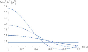
The angular profile for the vacuum polarization, neglecting the arbitrary term proportional to $R$, is depicted in Figure 1. Notice that in the absence of rotation spherical symmetry is recovered, with its value $\langle\phi^{2}\rangle_{r_{+}}^{Sch_{sub}}=(768\pi^{2}M^{2})^{-1}$ matching the result obtained in Cvetic:2014eka for the subtracted Schwarzschild black hole. In addition, the result at the pole takes the form $\langle\phi^{2}\rangle_{r_{+},\theta=0}=(768\pi^{2}M^{2})^{-1}(1+\alpha^{2})(1+4\alpha^{2}-\alpha^{4})$, agreeing with result found in Cvetic:2014eka using a non-corotating vacuum state (at the pole, the distinction is irrelevant). The dot-dashed plot corresponds to the extremal case $a=M$.

It would be interesting to compare our results with numerical computations of the vacuum polarization in the standard Kerr metric (with a mirror in place to define the vacuum). Our calculation holds for the minimally coupled field, and the numerical results in Duffy:2005mz are for the conformal case, so a direct comparison is not yet available. We expect our calculations to be easily generalized to the case of fields with higher spins as well as to rotating charged black holes, including multi-charged solutions Cvetic:1996kv ; Cvetic:1996xz ; Chow:2013tia . We also expect our methods to be applicable to the computation of the stress-energy tensor, which would open the possibility of using the subtracted approximation to study analytically the backreaction for rotating four-dimensional black holes.

Acknowledgements

We thank Finn Larsen and Gary Gibbons for valuable discussions and collaborations on related topics. MC would like to thank the organizers of the 2015 Mitchell Institute Workshop at the Great Brampton House for hospitality during the course of the work. The work is supported in part by the DOE (HEP) Award DE-SC0013528, the Fay R. and Eugene L. Langberg Endowed Chair (MC), and the Slovenian Research Agency (ARRS) (MC).

References

- (1) S. W. Hawking, “Particle Creation by Black Holes,” Commun. Math. Phys. 43, 199 (1975) [Commun. Math. Phys. 46, 206 (1976)].
- (2) P. Candelas, “Vacuum Polarization in Schwarzschild Space-Time,” Phys. Rev. D 21, 2185 (1980).
- (3) P. R. Anderson, “A method to compute in asymptotically flat, static, spherically symmetric space-times,” Phys. Rev. D 41, 1152 (1990).
- (4) A. Flachi and T. Tanaka, “Vacuum polarization in asymptotically anti-de Sitter black hole geometries,” Phys. Rev. D 78, 064011 (2008) [arXiv:0803.3125 [hep-th]].
- (5) A. C. Ottewill and P. Taylor, “Renormalized Vacuum Polarization and Stress Tensor on the Horizon of a Schwarzschild Black Hole Threaded by a Cosmic String,” Class. Quant. Grav. 28, 015007 (2011) [arXiv:1010.3943 [gr-qc]].
- (6) V. P. Frolov, “Vacuum Polarization Near The Event Horizon Of A Charged Rotating Black Hole,” Phys. Rev. D 26, 954 (1982).
- (7) G. Duffy and A. C. Ottewill, “The Renormalized stress tensor in Kerr space-time: Numerical results for the Hartle-Hawking vacuum,” Phys. Rev. D 77, 024007 (2008) [gr-qc/0507116].
- (8) A. Belokogne and A. Folacci, “Renormalized stress tensor for massive fields in Kerr-Newman spacetime,” Phys. Rev. D 90, no. 4, 044045 (2014) [arXiv:1404.7422 [gr-qc]].
- (9) C. Krishnan, “Black Hole Vacua and Rotation,” Nucl. Phys. B 848, 268 (2011) [arXiv:1005.1629 [hep-th]].
- (10) H. R. C. Ferreira and J. Louko, “Renormalized vacuum polarization on rotating warped black holes,” Phys. Rev. D 91, no. 2, 024038 (2015) [arXiv:1410.5983 [gr-qc]].
- (11) M. Cvetič and F. Larsen, “Conformal Symmetry for General Black Holes,” JHEP 1202, 122 (2012) [arXiv:1106.3341 [hep-th]];
- (12) M. Cvetič and F. Larsen, “Conformal Symmetry for Black Holes in Four Dimensions,” JHEP 1209, 076 (2012) [arXiv:1112.4846 [hep-th]];
- (13) M. Cvetič and G. W. Gibbons, “Conformal Symmetry of a Black Hole as a Scaling Limit: A Black Hole in an Asymptotically Conical Box,” JHEP 1207, 014 (2012) [arXiv:1201.0601 [hep-th]].
- (14) M. Cvetič and F. Larsen, “Black Holes with Intrinsic Spin,” JHEP 1411, 033 (2014) [arXiv:1406.4536 [hep-th]].
- (15) A. Castro, A. Maloney and A. Strominger, “Hidden Conformal Symmetry of the Kerr Black Hole,” Phys. Rev. D 82, 024008 (2010) [arXiv:1004.0996 [hep-th]].
- (16) G. Compère, “The Kerr/CFT correspondence and its extensions: a comprehensive review,” Living Rev. Rel. 15, 11 (2012) [arXiv:1203.3561 [hep-th]].
- (17) M. Cvetič, G. W. Gibbons and Z. H. Saleem, “Thermodynamics of Asymptotically Conical Geometries,” Phys. Rev. Lett. 114, 231301 (2015) [arXiv:1412.5996 [hep-th]].
- (18) M. Cvetič, Z. H. Saleem and A. Satz, “Entanglement entropy of subtracted geometry black holes,” JHEP 1409, 041 (2014) [arXiv:1407.0310 [hep-th]].
- (19) M. Cvetič, G. W. Gibbons, Z. H. Saleem and A. Satz, “Vacuum Polarization of STU Black Holes and their Subtracted Geometry Limit,” JHEP 1501, 130 (2015) [arXiv:1411.4658 [hep-th]].
- (20) M. Cvetič and G. W. Gibbons, “Exact quasinormal modes for the near horizon Kerr metric,” Phys. Rev. D 89, no. 6, 064057 (2014) [arXiv:1312.2250 [gr-qc]].
- (21) M. Cvetič, G. W. Gibbons and Z. H. Saleem, “Quasinormal modes for subtracted rotating and magnetized geometries,” Phys. Rev. D 90, no. 12, 124046 (2014) [arXiv:1401.0544 [hep-th]].
- (22) B. S. Kay and R. M. Wald, “Theorems on the Uniqueness and Thermal Properties of Stationary, Nonsingular, Quasifree States on Space-Times with a Bifurcate Killing Horizon” Phys. Rept. 207, 49 (1991).
- (23) A. C. Ottewill and E. Winstanley, “The Renormalized stress tensor in Kerr space-time: general results,” Phys. Rev. D 62, 084018 (2000) [gr-qc/0004022].
- (24) V. P. Frolov and K. S. Thorne, “Renormalized Stress - Energy Tensor Near the Horizon of a Slowly Evolving, Rotating Black Hole,” Phys. Rev. D 39, 2125 (1989).
- (25) I. S. Gradshteyn and I. M. Ryzhik A. Jeffrey (Ed.), Table of Integrals, Series and Products (5th ed.), Academic Press, New York (1994).
- (26) G. Sansone, Orthogonal Functions, Interscience, London (1959).
- (27) S. M. Christensen, “Vacuum Expectation Value of the Stress Tensor in an Arbitrary Curved Background: The Covariant Point Separation Method,” Phys. Rev. D 14, 2490 (1976).
- (28) J. Gustafson “Asymptotic formulas for elliptic integrals” PhD Thesis, Iowa State University (1982).
- (29) A. C. Ottewill and B. Wardell, “Quasi-local contribution to the scalar self-force: Non-geodesic Motion,” Phys. Rev. D 79, 024031 (2009) [arXiv:0810.1961 [gr-qc]].
- (30) M. Cvetič and D. Youm, “Entropy of nonextreme charged rotating black holes in string theory,” Phys. Rev. D 54 (1996) 2612 [hep-th/9603147].
- (31) M. Cvetič and D. Youm, “General rotating five-dimensional black holes of toroidally compactified heterotic string,” Nucl. Phys. B 476 (1996) 118 [hep-th/9603100].
- (32) D. D. K. Chow and G. Compère, “Seed for general rotating non-extremal black holes of supergravity,” Class. Quant. Grav. 31, 022001 (2014) [arXiv:1310.1925 [hep-th]].