Toward Simulation-free Estimation of Critical Clearing Time

Abstract

Contingency screening for transient stability of large scale, strongly nonlinear, interconnected power systems is one of the most computationally challenging parts of Dynamic Security Assessment and requires huge resources to perform time-domain simulations-based assessment. To reduce computational cost of time-domain simulations, direct energy methods have been extensively developed. However, these methods, as well as other existing methods, still rely on time-consuming numerical integration of the fault-on dynamics. This task is computationally hard, since possibly thousands of contingencies need to be scanned and thousands of accompanied fault-on dynamics simulations need to be performed and stored on a regular basis. In this paper, we introduce a novel framework to eliminate the need for fault-on dynamics simulations in contingency screening. This simulation-free framework is based on bounding the fault-on dynamics and extending the recently introduced Lyapunov Function Family approach for transient stability analysis of structure-preserving model. In turn, a lower bound of the critical clearing time (CCT) is obtained by solving convex optimization problems without relying on any time-domain simulations. A comprehensive analysis is carried out to validate this novel technique on a number of IEEE test cases.

I Introduction

Transient stability assessment, concerned with power systems stability/instability after contingencies, is a core element of the Dynamic Security Assessment Systems monitoring and allowing the reliable operation of power systems around the world. The most straightforward and dominant approach in industry to this problem is based on the direct time-domain simulations of transient post-fault dynamics following possible contingencies. Rapid advances in computational hardware enable it to perform accurate simulations of large scale systems possibly faster than real-time [1, 2]. However, in practice there are usually thousands to millions of contingencies that need to be screened on a regular basis. As such, the computational cost for time-domain simulations-based transient stability assessment is huge. At the same time, most of these contingencies are not critical, and thus most of computational resources are spent for assessment of contingencies that do not contribute to overall system risk.

To avoid time-consuming numerical integration of post-fault dynamics and save the computational resources, the smarter way nowadays is to use a combination of the direct energy approaches and time-domain simulation [3, 4, 5], in which most contingencies will be screened by the energy method and the remaining contingencies are checked by time-domain simulations. The advantage of direct energy method is that it allows fast screening of contingencies while providing mathematically rigorous certificates of stability. After decades of research and development, the controlling unstable equilibrium point (UEP) method [6] has been widely accepted as the most successful method among other energy function based direct screening methods, and is being applied in industry. This method is based on comparing the post-fault energy with the energy at the controlling UEP to certify transient stability.

The noticeable drawback of the controlling UEP method is the inherent difficulty of directly identifying the controlling UEP [7]. The controlling UEP is defined as the first UEP whose stable manifold is hit by the fault-on trajectory at the exit point, i.e. the point where the fault-on trajectory meets the actual stability boundary of the post-fault Stable Equilibrium Point (SEP). Note that the actual stability boundary of the SEP is generally unknown, and thus the computation of the exit point is very complicated and usually necessitates iterative time-domain simulations. For a given fault-on trajectory, the controlling UEP computation requires solving a large set of nonlinear differential algebraic equations which is done by numerical methods. However, with respect to these methods, e.g. Newton method, the convergence region of the controlling UEP can be very small and irregular compared to that of the SEP. If an initial guess for the numerical solver was not sufficiently close to the controlling UEP, then the computational algorithm will result in wrong controlling UEP and might probably converge to a SEP, leading to unreliable stability assessment. Unfortunately, it is extremely hard to find an initial guess sufficiently close to the controlling UEP.

The second drawback of the controlling UEP method is that it requires simulating and storing each fault-on trajectory to carry out the assessment for the respective contingencies. To the best of our knowledge, there are only a few works on contingency screening without relying on fault-on dynamics simulations. Particularly, in [8] the closest UEP method is exploited and an algebraic formulation of the critical clearing time is obtained based on polynomial approximation of the swing equations. However it is assumed that the dynamics of the rotor angles during the fault is a constant positive acceleration. This approximation is remarkable and may cause incorrect estimation of the critical clearing time.

The objective of this paper is to develop novel numerical approach that can potentially alleviate the computational burden of finding the controlling UEP. We aim to achieve this objective by developing a completely simulation-free technique for the estimation of critical clearing time. This technique is based on an extension of the recently introduced Lyapunov Functions Family (LFF) approach [9]. The principle of this approach is to provide transient stability certificates by constructing a family of Lyapunov functions and then finding the best suited function in the family for given initial states. Basically, this method certifies that the post-fault dynamics is stable if the fault-cleared state stays within a polytope surrounding the post-fault equilibrium point and the Lyapunov function at the fault-cleared state is smaller than the minimum value of Lyapunov function over the flow-out boundary of that polytope. Therefore, to screen the contingencies for transient stability, this method only requires the knowledge of the fault-cleared state, instead of the whole fault-on trajectory.

Exploiting this advantage of LFF method, a technique is introduced to bound the fault-on dynamics and thereby the fault-cleared state. This bound leads to a transient stability certificate that only relies on checking the clearing time, i.e. if the clearing time is under certain threshold then the fault-cleared state is still in the region of attraction of the original SEP and the post-fault dynamics is determined stable. By this new method, a fast transient stability assessment for a large number of contingencies can be obtained without using any simulations. Such approach can be utilized in several power system applications, such as optimal power flow, resources allocation, and HVDC control problems [10, 11, 12, 13, 14, 15, 16, 17], where the proposed transient stability certificate can help reduce the search space by eliminating less critical contingencies in studies.

The structure of this paper is as follows. In Section II the contingency screening problem addressed in this paper is introduced, together with the extension of the LFF approach for transient stability analysis. Section III presents the main result of this paper regarding the simulation-free algebraic estimation of the critical clearing time, and explains how this new stability certificate can be used in practice to screen contingency for transient stability without any time-domain simulations. Finally, in Section IV performance of the proposed method on contingency screening of several IEEE test systems is presented and analyzed. Section V concludes the paper with discussions about possible ways to improve the algorithms.

II Lyapunov Function Family Approach for Transient Stability

In this section, we show that the Lyapunov function family approach [9], originally presented for the Kron-reduction model, is applicable to the transient stability analysis of structure-preserving power models. Then, we extend this family to a set of convex Lyapunov functions family, that will be instrumental to establish a lower bound of critical clearing time in the next section.

In normal conditions, power grids operate at some stable equilibrium point. During disturbances such as faults, the system evolves subject to the fault-on (disturbance) dynamics and moves away from the pre-fault equilibrium point. After the fault is cleared, the system may return back to the pre-fault SEP or to a new post-fault SEP depending on whether the fault is self-cleared or cleared by circuit breakers action. In this paper, the proposed method tackles the type of contingencies, where a fault occurs in a transmission line and then self clears such that the post-fault network recovers to the pre-fault network topology. To describe the post-fault dynamics, we utilize the differential structure-preserving model [18]. This model naturally incorporates the dynamics of rotor angle as well as response of dynamic load power output to frequency deviation. Though it does not model the dynamics of voltage in the system, in comparison to the Kron-reduction models with constant impedance loads [19], the structure of power systems and the impact of load dynamics are preserved in this approach. When the losses of the transmission lines are ignored, the model can be expressed as:

$$m_{k}\ddot{\delta_{k}}+d_{k}\dot{\delta_{k}}+\sum_{j\in\mathcal{N}_{k}}a_{kj}\sin(\delta_{k}-\delta_{j})= P_{m_{k}},$$ (1)

$$k=1,\dots,m,$$

$$d_{k}\dot{\delta_{k}}+\sum_{j\in\mathcal{N}_{k}}a_{kj}\sin(\delta_{k}-\delta_{j})= -P^{0}_{d_{k}},$$ (2)

$$k=m+1,\dots,n,$$

where the first $m$ equations represent the dynamics of generators and the remaining $(n-m)$ equations represent the dynamics of frequency-dependent loads. With $k=1,...,m,$ then $m_{k}$ is the dimensionless moment of inertia of the $k^{th}$ generator, $d_{k}$ is the term representing primary frequency controller action on the governor, and $P_{m_{k}}$ is the effective dimensionless mechanical power input acting on the rotor. With $k=m+1,...,n,$ then $d_{k}>0$ is the constant frequency coefficient of load and $P^{0}_{d_{k}}$ is the nominal load. Let $\mathcal{E}$ be the set of all the transmission lines and $\mathcal{N}_{k}$ be the set of neighboring buses of the bus $k^{th}.$ Then, $a_{kj}=V_{k}V_{j}B_{kj},$ where $[B_{kj}]_{\{k,j\}\in\mathcal{E}}$ is the susceptance matrix and $V_{k}$ represents the voltage magnitude at the $k^{th}$ bus, both of which are assumed to be constant. The stationary operating condition is given by $[\delta_{1}^{*},\dots,\delta_{n}^{*},0,\dots,0]^{T}$ where $\delta_{k}$ is solution of the power flow-like equations

$$\sum_{j\in\mathcal{N}_{k}}a_{kj}\sin(\delta_{k}-\delta_{j})=P_{k},\forall k=1,\dots,n,$$ (3)

where $P_{k}=P_{m_{k}},k=1,\dots,m,$ and $P_{k}=-P^{0}_{d_{k}},k=m+1,\dots,n.$ We assume that there exists a stable operating condition $\delta^{*}\in\Delta(\lambda),\lambda<\pi/2,$ where the polytope $\Delta(\lambda)$ is defined by inequalities $|\delta_{kj}|\leq\lambda$ for all $\{k,j\}\in\mathcal{E}.$

In the LFF approach, the nonlinear couplings and the linear model are separated. To do that, the state vector $x=[x_{1},x_{2},x_{3}]^{T}$ is introduced which is composed of the vector of generator’s angle deviations from equilibrium $x_{1}=[\delta_{1}-\delta_{1}^{*},\dots,\delta_{m}-\delta_{m}^{*}]^{T}$, their angular velocities $x_{2}=[\dot{\delta}_{1},\dots,\dot{\delta}_{m}]^{T}$, and the vector of load’s angle deviation from equilibrium $x_{3}=[\delta_{m+1}-\delta_{m+1}^{*},\dots,\delta_{n}-\delta_{n}^{*}]^{T}$. Let $E$ be the incidence matrix of the corresponding graph, so that $E[\delta_{1}\dots\delta_{n}]^{T}=[(\delta_{k}-\delta_{j})_{\{k,j\}\in\mathcal{E}}]^{T}$. Consider matrix $C$ such that $Cx=E[\delta_{1}\dots\delta_{n}]^{T}.$ Consider the vector of nonlinear power flow $F$ in the simple trigonometric form $F(Cx)=[(\sin\delta_{kj}-\sin\delta^{*}_{kj})_{\{k,j\}\in\mathcal{E}}]^{T}.$

Then, in state space representation the system can be expressed in the following compact form:

$$\dot{x}_{1} =x_{2}$$

$$\dot{x}_{2} =M_{1}^{-1}D_{1}x_{2}-S_{1}D^{-1}E^{T}SF(Cx)$$ (4)

$$\dot{x}_{3} =-S_{2}D^{-1}E^{T}SF(Cx)$$

where $S=\emph{\emph{diag}}(a_{kj})_{\{k,j\}\in\mathcal{E}}$ is the diagonal matrix of coupling magnitudes and $S_{1}=[I_{m\times m}\quad O_{m\times n-m}],S_{2}=[O_{n-m\times m}\quad I_{n-m\times n-m}],D_{1}=\emph{\emph{diag}}(d_{1},\dots,d_{m}),M_{1}=\emph{\emph{diag}}(m_{1},\dots,m_{n}),D=\emph{\emph{diag}}(m_{1},\dots,m_{m},d_{m+1},\dots,d_{n}).$ Equivalently,

$$\dot{x}=Ax-BF(Cx),$$ (5)

with the matrices $A,B$ given by the following expression:

$$A=\left[\begin{array}[]{ccccc}O_{m\times m}&I_{m\times m}&O_{m\times n-m}\\ O_{m\times m}&-M_{1}^{-1}D_{1}&O_{m\times n-m}\\ O_{n-m\times m}&O_{n-m\times m}&O_{n-m\times n-m}\end{array}\right],$$

and

$$B=\left[\begin{array}[]{ccccc}O_{m\times|\mathcal{E}|};\quad S_{1}D^{-1}E^{T}S;\quad S_{2}D^{-1}E^{T}S\end{array}\right].$$ (7)

Here, $|\mathcal{E}|$ is the number of edges in the graph defined by the susceptance matrix, or equivalently the number of non-zero non-diagonal entries in $B_{kj}$.

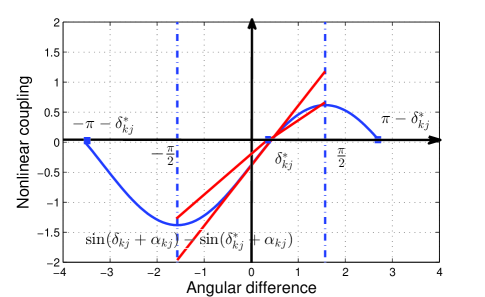
Figure 1: Strict bounding of the nonlinear function $f_{kj}$ by linear functions of the angular difference $(\delta_{kj}-\delta^{*}_{kj})$ in the lossy power systems

For the system defined by (5), the LFF approach proposes to use the Lyapunov functions family given by:

$$V(x)=\frac{1}{2}x^{T}Qx-\sum_{\{k,j\}\in\mathcal{E}}K_{\{k,j\}}\left(\cos\delta_{kj}+\delta_{kj}\sin\delta_{kj}^{*}\right)$$ (8)

in which the diagonal, nonnegative matrices $K,H$ and the symmetric, nonnegative matrix $Q$ satisfy the following linear matrix inequality (LMI):

$$\left[\begin{array}[]{ccccc}A^{T}Q+QA&R\\ R^{T}&-2H\\ \end{array}\right] \leq 0,$$ (11)

with $R=QB-C^{T}H-(KCA)^{T}$. Then, it can be proved that the Lyapunov function is decreasing in the polytope $\mathcal{P}$ defined by inequalities $|\delta_{kj}+\delta_{kj}^{*}|\leq\pi,\forall\{k,j\}\in\mathcal{E}.$ In order to ensure that the system will not escape the polytope $\mathcal{P}$ during transient dynamics one condition will be added to restrict the set of initial states inside $\mathcal{P}.$ Accordingly, we define the minimization of the function $V(x)$ over the union $\partial\mathcal{P}^{out}$ of the flow-out boundary segments $\partial\mathcal{P}_{kj}^{out}$ as follows:

$$V_{\min}=\mathop{\min}\limits_{x\in\partial\mathcal{P}^{out}}V(x),$$ (12)

where $\partial\mathcal{P}_{kj}^{out}$ is the flow-out boundary segment of polytope $\mathcal{P}$ that is defined, for each transmission line $\{k,j\}\in\mathcal{E}$ connecting generator buses $k$ and $j,$ by $|\delta_{kj}+\delta_{kj}^{*}|=\pi$ and $\delta_{kj}\dot{\delta}_{kj}\geq 0$. Given the value of $V_{\min},$ an LFF-based estimation for the region of attraction of the equilibrium point is given by

$$\mathcal{R_{P}}=\left\{x\in\mathcal{P}:V(x)<V_{\min}\right\}.$$ (13)

Finally, to determine if the post-fault dynamics is stable, we check if the fault-cleared state $x_{0}$ is inside the stability region estimate $\mathcal{R_{P}}$, i.e. if $x_{0}$ is in the polytope $\mathcal{P}$ and $V(x_{0})<V_{\min}.$ Therefore, to certify transient stability of each contingency, the LFF approach only need to know the fault-cleared state $x_{0}$ (i.e. the state of fault-on trajectory at the clearing time), rather than the whole fault-on trajectory.

In this paper, the proposed approach is only concerned with voltage phase angles staying inside the polytope $\mathcal{Q}$ defined by inequalities $|\delta_{kj}|\leq\pi/2,\forall\{k,j\}\in\mathcal{E}.$ An advantage of considering this polytope of voltage phasor angles is that inside this polytope the Lyapunov function $V(x)$ defined in (8) is convex. As such, the minimum value $V_{\min}$ can be calculated in polynomial time. In addition, inside this polytope, a stricter bounding for the nonlinear flow vector $F$ can be established as follows

$$(f_{\{k,j\}}-(\delta_{kj}-\delta_{kj}^{*}))(f_{\{k,j\}}-\beta(\delta_{kj}-\delta_{kj}^{*}))\leq 0$$ (14)

where $\beta=\dfrac{1-\sin\lambda}{\pi/2-\lambda}>0$ and $f_{\{k,j\}}=\sin\delta_{kj}-\sin\delta_{kj}^{*}$ is an element of the vector $F.$ Exploiting this strict bound of the nonlinear flow vector $F,$ the LMI (11) can be replaced by the following less restrictive LMI:

$$\left[\begin{array}[]{ccccc}A^{T}Q+QA-2\beta C^{T}HC&\tilde{R}\\ \tilde{R}^{T}&-2H\\ \end{array}\right]\leq 0,$$ (17)

$$\tilde{R}=QB-(1+\beta)C^{T}H-(KCA)^{T},$$

while all the above results for the stability certificate still hold true. In particular, the estimate for region of attraction is given by

$$\mathcal{R_{Q}}=\left\{x\in\mathcal{Q}:V(x)<V_{\min}\right\}$$ (18)

with

$$V_{\min}=\mathop{\min}\limits_{x\in\partial\mathcal{Q}^{out}}V(x).$$ (19)

The proof of this fact is given in Appendix VI-A. With the less restrictive LMI (17), a broader family of Lyapunov functions can be obtained, which will be exploited to establish the lower bound of the critical clearing time in the next section.

Remark 1

The main drawback of the proposed stability certificate is that it currently does not incorporate the detailed model of generators and its associate control systems, such as excitation systems, PSS and governor system. Swing equation model doesn’t incorporate associated control systems and generator’s fast dynamics and assumes a fixed field voltage magnitude during transient period. However, the setpoint values of voltage magnitude can be allowed to fluctuate around the nominal value $V_{0}$ (let say less than $10\%$ around $V_{0}$). In the matrix $B$ in (7), we take the new the coupling magnitude diagonal matrix $S=\emph{\emph{diag}}(1.1^{2}V_{0}^{2}B_{kj})_{\{k,j\}\in\mathcal{E}}.$ Consider the new nonlinear vector $F=[f_{kj}]_{\{k,j\}\in\mathcal{E}}$ where

$$f_{kj}=\frac{V_{k}V_{j}(\sin\delta_{kj}-\sin\delta^{*}_{kj})}{1.1^{2}V_{0}^{2}}$$ (20)

We can see that the bounding for nonlinear function $f_{kj}$ in (14) still holds true with $\beta$ replaced by the smaller value $0.9^{2}\beta/1.1^{2}.$ Then, all the other results will follow accordingly. As such, the simple Lyapunov function (8) and stability region estimate (18) can be easily extended to the case when voltage magnitude setpoints fluctuate $10\%$ around the nominal value. In this case, since we have looser bounding for the nonlinear vector $F,$ the according stability region estimate will be smaller than the original defined in (18). Therefore, the proposed framework can manifest the fact that the stability region is smaller due to the effects of generators’ control systems (however, it cannot capture the voltage collapse phenomenon when the voltage magnitudes sag to the low values). From this analysis, we suggest that in the practical transient stability assessment, we should accordingly modify the estimation of the stability region to avoid overestimation of the CCT due to the usage of simple generators’ model.

Remark 2

Since the proposed stability certificate only requires the Lyapunov function to be locally decreasing, rather than decreasing in the whole state space as in the energy method, the LFF framework can be extended to incorporate the losses in transmission lines. Indeed, the stability analysis here is essentially based on bounding the nonlinear function $f_{kj}$ by linear functions of $\delta_{kj}$ as in (14), i.e. whenever the bounding (14) holds true, we can have the stability region estimate accordingly. For the power systems with losses, we take the coupling magnitude diagonal matrix $S=\emph{\emph{diag}}(V_{k}V_{j}Y_{kj})_{\{k,j\}\in\mathcal{E}}$ and the nonlinear function $f_{kj}$ as

$$f_{kj}=(\sin(\delta_{kj}+\alpha_{kj})-\sin(\delta^{*}_{kj}+\alpha_{kj})$$ (21)

Here, $Y_{kj}=\sqrt{G_{kj}^{2}+B_{kj}^{2}}$ and $\alpha_{kj}=\arctan(G_{kj}/B_{kj})\ll 1,$ where $G_{kj}$ and $B_{kj}$ are the (normalized) conductance and susceptance of the transmission line $\{k,j\}.$ From Fig. 1, we can show that the nonlinear bounding (14) still holds true for any $x\in\mathcal{Q}$ and

$$\beta=\min_{\{k,j\}\in\mathcal{E}}\frac{\sin(\pi/2+\alpha_{kj})-\sin(|\delta^{*}_{kj}|+\alpha_{kj})}{\pi/2-|\delta_{kj}^{*}|}$$ (22)

Then, all the stability analysis follows accordingly. Therefore, the LFF framework and the CCT estimation to be presented in the next section is applicable to lossy power systems. We will illustrate the proposed framework for estimating CCT of the lossy 2-bus system in Section IV.A.

III Contingency Screening without Time-domain Simulations

In this section, we present a new approach to the contingency screening problem, which relies on a combination the LFF framework introduced in the previous section and the bounding for the reachability set of the fault-on dynamics, through which we can guarantee that the fault-cleared state is still inside the region of attraction of the post-fault stable equilibrium point. Interestingly, this bound leads to an algebraic simulation-free lower bound of the critical clearing time. Therefore, this contingency screening approach completely removes any time-domain simulations of both the post-fault dynamics and fault-on dynamics.

III-A Bounding for The Fault-on Dynamics

If the time-domain simulation for fault-on dynamics is used, the fault-cleared state $x_{0}$ can be determined by directly integrating the fault-on dynamics. Then, the value of $V_{0}=V(x_{0})$ computed from (8) is compared to the value of $V_{\min}$ to certify transient stability.

Now, assume that time-domain simulations are not used to integrate the fault-on dynamics. Then the fault-cleared state $x_{0}$ will not be known precisely. To guarantee that $x_{0}\in\mathcal{Q}$ and $V(x_{0})<V_{\min},$ we will bound the fault-on dynamics. Consider the normal condition when the pre-fault system is in the stable operating condition defined by the stable equilibrium point $\delta^{*}_{pre}\in\Delta(\lambda).$ Assume that a fault occurs at the transmission line $\{u,v\}\in\mathcal{E}$ and then self-clears such that the power network recovers to its pre-fault topology. During the fault, the power system dynamics is approximated by equations:

$$\dot{x}_{F}=Ax_{F}-BF_{pre}(Cx_{F})+BD_{\{u,v\}}\sin\delta_{{uv}_{F}}$$ (23)

Here, the fault-on trajectory is denoted as $x_{F}(t)$ to differentiate it from the post-fault trajectory $x(t)$ in (5). $D_{\{u,v\}}$ is the unit vector to extract the nonlinear function $(\sin\delta_{{uv}_{F}}-\sin\delta^{*}_{{uv}_{pre}})$ from the nonlinear vector $F_{pre}=[(\sin\delta_{{kj}_{F}}-\sin\delta^{*}_{{kj}_{pre}})]_{\{k,j\}\in\mathcal{E}}$, which serves to model the elimination of the faulted line $\{u,v\}$ during the fault. In Appendix VI-B, the following center result regarding the bounding of the fault-on dynamics is proven, which will be instrumental to the introduction of stability certificate in the next section. If there exist matrices $Q,K,H,H\geq 0$ and a positive number $\gamma$ such that

$$\left[\begin{array}[]{ccccc}\tilde{A}+\gamma(QBD_{\{u,v\}})(QBD_{\{u,v\}})^{T}&\tilde{R}\\ \tilde{R}^{T}&-2H\\ \end{array}\right] \leq 0,$$ (26)

where $\tilde{A}=A^{T}Q+QA-2\beta C^{T}HC,\tilde{R}=QB-(1+\beta)C^{T}H-(KCA)^{T}$, then along the fault-on dynamics (23) we have $\dot{V}(x_{F}(t))\leq\dfrac{1}{2\gamma}$ whenever $x_{F}(t)$ being in the polytope $\mathcal{Q}.$

Note that due to (26), the Lyapunov function’s derivative $\dot{V}(x)$ along the post-fault dynamics (5) is non-positive in the polytope $\mathcal{Q}.$ Basically, the above result provides a certificate to make sure that the fault-on dynamics does not deviate too much from the post-fault dynamics. As such, if the clearing time is under some threshold, then the fault-cleared state (i.e. the state of fault-on system at the clearing time) is not very far from the considered working condition. The above result as such is essential to establish a lower bound of the critical clearing time in the next section.

III-B Estimation of The Critical Clearing Time

Let the clearing time be $\tau_{clearing}.$ In Appendix VI-C, the following stability certificate which only relies on checking the clearing time is proven. If the inequality (26) holds and the clearing time $\tau_{clearing}$ satisfies $\tau_{clearing}<2\gamma(V_{\min}-V(x_{pre})),$ where $x_{pre}=\delta^{*}_{pre}-\delta^{*}_{post},$ then, the fault-cleared state $x_{F}(\tau_{clearing})$ is still inside the region of attraction of the post-fault SEP $\delta^{*}_{post}$ and the post-fault dynamics following the considered contingency leads to the stable operating condition $\delta^{*}_{post}$.

Therefore, this stability certificate provides us with a lower bound of the critical clearing time as $2\gamma(V_{\min}-V(x_{pre}))$ obtained by solving the inequality (26). This estimation is totally simulation-free, distinguishing it from other methods in the literature to estimate the critical clearing time.

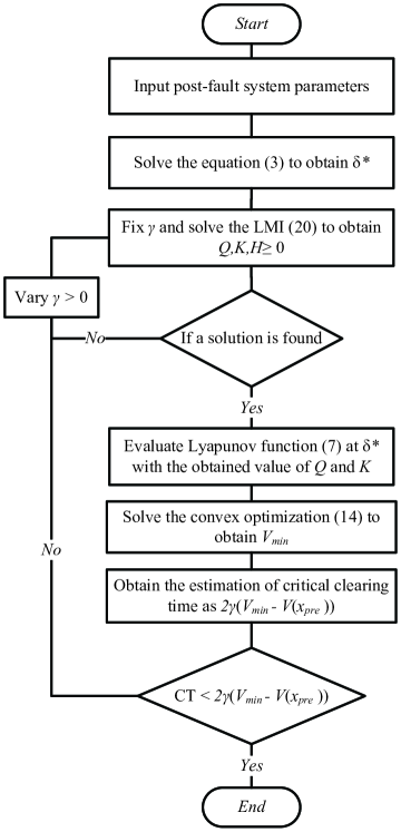
Figure 2: Algorithm to screen contingencies for transient stability without simulations of fault-on dynamics and post-fault dynamics

We note that it is also possible to extend this stability certificate to the case when several contingencies co-exist. This case is of practical interest. Indeed, the large-area blackout in practice is usually a result of multiple contingencies happening at short time interval. Though large-area blackout is rare, its effect is severe, both economically and humanly. Therefore, it is critical to check if the power grids stand when several contingencies are happening, or leading to large-area blackout. The technique presented in this paper provides a framework to certify the safety of power grids.

III-C Choosing Lyapunov Function and Parameter $\gamma$

Since there is a family of Lyapunov functions $V(x),$ characterized by matrices $Q,K,$ and positive numbers $\gamma$ that satisfy the inequality (26), we have different estimations $2\gamma(V_{\min}-V(x_{pre}))$ of the critical clearing time (CCT). To get the highest possible estimation of the CCT, we need to find the maximum value of $2\gamma(V_{\min}-V(x_{pre}))$ over all the matrices $Q,K$ and positive numbers $\gamma$ satisfying (26). Unfortunately, this is an NP-hard, strongly nonlinear optimization problem with both nonlinear objective function and nonlinear constraint.

We observe that a good selection of Lyapunov function and the parameter $\gamma$ is obtained if we can predict the location of the fault-cleared state. In the following, we propose two procedures suggesting some directions to search for feasible Lyapunov function and parameter $\gamma$ allowing for good estimation of the CCT. The first procedure is totally heuristic, where we vary $\gamma$ and find the corresponding Lyapunov function. The second one is based on a prediction of the fault-cleared state. Both of these procedures rely on solving a number of convex optimization problems in the form of either quadratic programming or semidefinite programming.

Procedure 1: To solve the inequality (26), we note that for a fixed value of $\gamma,$ the inequality (26) can be transformed to the following LMI of the matrices $Q,K,H$ via Schur complement:

$$\left[\begin{array}[]{ccccc}A^{T}Q+QA-2\beta C^{T}HC&(\sqrt{\gamma}(QBD_{\{u,v\}})\;\;\tilde{R})\\ (\sqrt{\gamma}(QBD_{\{u,v\}})\;\;\tilde{R})^{T}&-L\\ \end{array}\right] \leq 0,$$ (29)

where $L=\left[\begin{array}[]{ccccc}I&O\\ O&2H\\ \end{array}\right].$ The matrices $Q,K,H$ can be found quickly from the LMI (29) by convex optimization. Therefore, a heuristic algorithm can be used to find solution of (26), in which $\gamma$ is varied and the LMI (29) is solved to obtain the matrices $Q,K,H$ accordingly.

Procedure 2:

• Calculate the distance $r$ from the equilibrium point $\delta^{*}_{post}$ to the boundary of the polytope $\mathcal{Q}$ as $r=\min_{\delta\in\partial\mathcal{Q}}||\delta-\delta^{*}_{post}||_{2}.$

• Take $k$ points $x_{1},...,x_{k}$ uniformly distributed on the sphere $S=\{\delta:||\delta-\delta^{*}_{post}||_{2}=r\}$ which surrounds $\delta^{*}_{post}$ and stays inside $\mathcal{Q}.$ These points are considered as possible predictions for the fault-cleared state.

• For each point $x_{i},$ using the adaptation algorithm proposed in [9] to find a Lyapunov function $V_{i}(x)$ characterized by matrices $Q_{i},K_{i}$ such that the point $x_{i}$ stays inside the stability region estimate $\mathcal{R_{Q}}$ defined in (18). This adaptation algorithm can quickly find a suitable Lyapunov function after a finite number of steps.

• For the matrices $Q_{i},K_{i},$ find the maximum value $\gamma^{*}_{i}$ satisfying the inequality (26) as: $\gamma^{*}_{i}=\max\gamma$ subject to (26) where $Q=Q_{i},K=K_{i},H=H_{i}$. Calculate $\tau_{i}=2\gamma^{*}_{i}(V_{{\min}_{i}}-V_{i}(x_{pre})).$

• Take the estimation of the CCT as the maximum value out of $\tau_{1},...,\tau_{k}.$

We note that compared to Procedure 1, Procedure 2 may remarkably increase the computational complexity of calculating the CCT estimate. Recent studies shown that matrices appearing in power system context are characterized by graphs with low maximal clique order, and thus the related SDP in these procedures can be quickly solved by the new generation of SDP solvers [20, 21]. In addition, the advances in parallel computing, e.g. distributed computing with zero overhead communication, promises to significantly reduce the computational load for these SDP solvers.

III-D Contingency Screening without Simulations

The stability certificate in Section III.B provides us with a way to directly screen contingencies for transient stability assessment without any time-domain simulations, as described by the algorithm in Fig. 2. Basically, for the contingency manifested by the tripping of line $\{u,v\},$ one can check if the inequality (26) is solvable. In case it is solvable to find the matrices $Q,K,H,$ and the positive number $\gamma,$ then the Lyapunov function $V(x)$ can be derived as in (8), and the minimum value $V_{\min}$ defined in (19) can be calculated. Finally, if the clearing time (CT) $\tau_{clearing}$ satisfies that $\tau_{clearing}<2\gamma(V_{\min}-V(x_{pre})),$ where $x_{pre}=\delta^{*}_{pre}-\delta^{*}_{post},$ then we conclude that the post-fault dynamics following the considered contingency leads to a stable operating condition. If this inequality is not true, or if there is no solution for the inequality (26), then nothing can be concluded about the stability or instability of the post-fault dynamics. The contingency in this case should be screened by other energy method or by direct time-domain simulations.

In contingency screening, it is greatly advantageous if we have a certificate to screen any possible contingency associated with the tripping of any transmission line in the set $\mathcal{F}\subset\mathcal{E}$. Let $D$ be a matrix larger than or equal to $D_{\{u,v\}}D_{\{u,v\}}^{T}$ for all the lines $\{u,v\}\in\mathcal{F}.$ We have the following result for the robust screening of contingencies. If the inequality (26) holds with $D_{\{u,v\}}D_{\{u,v\}}^{T}$ replaced by $D$, and the clearing time $\tau_{clearing}$ satisfies $\tau_{clearing}<2\gamma(V_{\min}-V(x_{pre}))$, then, for any contingency associated with the tripping of any line $\{u,v\}\in\mathcal{F},$ the fault-cleared state $x_{F}(\tau_{clearing})$ is still inside the region of attraction of the post-fault SEP $\delta^{*}_{post}$, and the post-fault dynamics following the considered contingency leads to the stable operating condition $\delta^{*}_{post}$. This result is a straightforward corollary of the stability certificate in Section III-B, and thus its proof is omitted here.

IV Numerical Illustrations

IV-A Classical 2-Bus lossy System with Different Pre-fault and Post-fault SEPs

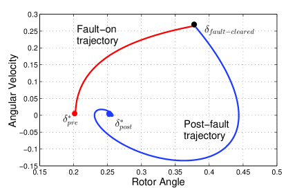
Figure 3: System trajectory according to the fault-on dynamics and post-fault dynamics with the clearing time $CT=2\gamma(V_{\min}-V(x_{pre}))=1.0600s$

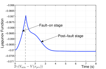
Figure 4: Dynamics of the Lyapunov function during the fault-on stage and post-fault stage with the clearing time $CT=2\gamma(V_{\min}-V(x_{pre}))=1.0600s$

For illustrating the presented concepts, this section presents the simulation results on the most simple 2-bus lossy power system, described by the single 2-nd order differential equation

$$m\ddot{\delta}+d\dot{\delta}+a\sin(\delta+\alpha)-p=0.$$ (30)

For numerical simulations, we choose $m=0.1$ p.u., $d=0.15$ p.u., $a=0.2$ p.u., and $\alpha=0.05$ rad. The pre-fault and post-fault power inputs are $p_{pre}=0.05$ p.u. and $p_{post}=0.06$ p.u. Then, the pre-fault and post-fault stable equilibrium point are given by $[\delta^{*}_{pre}\;\;0]^{T}=[0.2027\;\;0]^{T}$ and $[\delta^{*}_{post}\;\;0]^{T}=[0.2547\;\;0]^{T},$ both of which are in the polytope $\Delta(\pi/10).$ Hence, $\beta=(\sin(\pi/2+\alpha)-\sin(\pi/10+\alpha))/(\pi/2-\pi/10)=0.5114.$ By varying $\gamma$ and solving the LMI (29), we obtain the corresponding lower bounds for the critical clearing time as in Tab. I.

$\gamma$	$2\gamma(V_{\min}-V(x_{pre}))(s)$
1	0.9442
2	0.9757
3	1.0077
4	1.0297
5	1.0439
6	1.0535
7	1.0600
8	1.0578
9	1.0574
10	1.0553

TABLE I: Lower bound of the critical clearing time vs. $\gamma$

Therefore, in these values of $\gamma,$ with $\gamma=7$ we obtain the largest lower bound for the critical clearing time as $1.0600.$ The corresponding matrices $Q,K,H$ are

$$Q=\left[\begin{array}[]{ccccc}0.0443&0.0127\\ 0.0127&0.0879\\ \end{array}\right];K=0.0968;H=0.2412,$$ (33)

while the corresponding value of $V_{\min}-V(x_{pre})$ is $0.0528.$ In Fig. 3 we show the dynamics of the system trajectory in the fault-on and post-fault-stage in which the clearing time is taken as $\tau_{clearing}=2\gamma(V_{\min}-V(x_{pre}))=1.0600s.$ It can be seen that when the fault happens, the system evolves according to the fault-on dynamics and the system trajectory deviates from the pre-fault equilibrium point $\delta^{*}_{pre}$ to the fault-cleared state $\delta_{fault-cleared}.$ After the fault self-clears, the system trajectory recovers from the fault-cleared state $\delta_{fault-cleared}$ to the post-fault equilibrium point $\delta^{*}_{post}$ which is different from the pre-fault equilibrium. Figure 4 shows the divergence of the Lyapunov function during the fault-on stage and the convergence of Lyapunov function during the post-fault stage. These figures confirm the estimation of the critical clearing time as obtained by the proposed method in this paper.

IV-B Three Generator System

Consider the system of three generators with the time-invariant terminal voltages and mechanical torques given in Tab. II.

Node	V (p.u.)	$P_{k}$ (p.u.)
1	1.0566	-0.2464
2	1.0502	0.2086
3	1.0170	0.0378

TABLE II: Voltage and mechanical input

The susceptances of the transmission lines are $B_{12}=0.739$ p.u., $B_{13}=1.0958$ p.u., and $B_{23}=1.245$ p.u. The equilibrium point is calculated as: $\delta^{*}=[-0.6634\;-0.5046\;-0.5640\;0\;0\;0]^{T},$ which belongs to the polytope $\Delta(\pi/10).$ Hence, we can take $\beta=(1-\sin(\pi/10))/(\pi/2-\pi/10).$ For simplicity we just take $m_{k}=2,d_{k}=1,k=1,2,3.$ Assume that the fault happens at the transmission line connecting generators $1$ and $2$ and then self-clears. Also, during that time the mechanical inputs are assumed to be unchanged. Taking $\gamma=3$ and using CVX software we can solve the LMI (29) we obtain $Q$ as

$$\left[\begin{array}[]{cccccc}3.8376&3.8012&3.5779&7.5549&7.4619&7.4166\\ 3.8012&3.8457&3.5698&7.4776&7.5530&7.4029\\ 3.5779&3.5698&4.0690&7.4010&7.4185&7.6140\\ 7.5549&7.4776&7.4010&38.9402&38.2449&38.0704\\ 7.4619&7.5530&7.4185&38.2449&38.9534&38.0571\\ 7.4166&7.4029&7.6140&38.0704&38.0571&39.1280\\ \end{array}\right]$$ (40)

and $K=\emph{\emph{diag}}(0.2554,\;0.3638,\;0.4386),H=\emph{\emph{diag}}(0.0943,0.2533,0.2960).$ The corresponding estimation of the critical clearing time is $2\gamma(V_{\min}-V(x_{pre}))=0.2376s.$

IV-C Kundur 9-Bus 3-Generator System

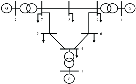
Figure 5: 3 generator 9 bus system with frequency-dependent dynamic loads

Consider the Kundur 9 bus 3 machine system depicted in Fig. 5 with 3 generator buses and 6 load buses. The susceptances of the transmission lines are as follows: $B_{14}=17.3611p.u.,B_{27}=16.0000p.u.,B_{39}=17.0648p.u.,B_{45}=11.7647p.u.,B_{57}=6.2112p.u.,B_{64}=10.8696p.u.,B_{78}=13.8889p.u.,B_{89}=9.9206p.u.,B_{96}=5.8824p.u.$ The bus voltages $V_{k}$, mechanical inputs $P_{m_{k}}$, and steady state load $-P_{d_{k}}^{0}$ are given in Tab. III. The stable operating condition is obtained by solving equations (3) as $x^{*}=[0.0381\;0.3208\;0.1924\;-0.0349\;-0.0421\;-0.0409\;0.0519\;0.0178\;0.0155\;0\;0\;0\;0\;0\;0\;0\;0\;0],$ which stays in the polytope $\Delta(\pi/8).$ Hence $\beta=(1-\sin(\pi/8))/(\pi/2-\pi/8)=0.5240.$ The parameters for generators are $m_{1}=0.1254,m_{2}=0.034,m_{3}=0.016,d_{1}=0.0627,d_{2}=0.017,d_{3}=0.008.$ For simplicity, we take $d_{k}=0.05,k=4\dots,9.$ Assume that the fault trips the line between buses $6$ and $4$ and when the fault is cleared this line is re-closed. With $\gamma=7.10^{-6},$ using the CVX software, we can solve the LMI (29) in 1s to obtain the Lyapunov function. Accordingly, we can calculate the minimum value of the Lyapunov function and obtain the estimation for the critical clearing time as $2\gamma(V_{\min}-V(x_{pre}))=0.1175s.$

Node	V (p.u.)	$P_{k}$ (p.u.)
1	1.0284	0.6700
2	1.0085	1.6300
3	0.9522	0.8500
4	1.0627	-0.5000
5	1.0707	-0.7500
6	1.0749	-0.4500
7	1.0490	-0.4500
8	1.0579	-0.5000
9	1.0521	-0.5000

TABLE III: Bus voltages, mechanical inputs and static loads

We perform time domain simulations to find the critical clearing time for the system when the generators are modeled by swing equations and by $4^{th}$ orders machine models incorporating generators’ control systems. Accordingly, we can find that when the fault happens at the transmission line $\{4,6\},$ the true critical clearing times for the swing model and $4^{th}$ orders machine models are, respectively, $0.25$s and $0.18$s. Therefore, the critical clearing time estimated by the proposed method in this paper is about half of the true one. We conclude that the proposed method is conservative in comparison to the time domain simulations, but there is no overestimation for the CCT. In addition, the time domain simulations confirm the analysis we described in Remark 1 that the generators’ control systems make the critical clearing time to reduce.

In comparison to the controlling UEP method, the proposed method in this paper is also more conservative since the controlling UEP was reported [5] to get the estimate for critical clearing time which is different in less than $10\%$ from the true one obtained by time domain simulation. However, we note that the CCT estimate proposed in this paper does not require time-domain simulation for the fault-on dynamics as in the controlling UEP method. This will help significantly reduce the computational resources spent for contingency screening. Therefore, the proposed framework in this paper can be considered as a complement of the time domain simulation method and controlling UEP method, which could be efficiently used when we aim to screen non-critical contingencies with little computational resources.

V Conclusions and Path Forward

In this paper, we introduced techniques to screen contingencies for transient stability without relying on any time-domain simulations. This is based on extending the recently introduced LFF transient stability certificate in the combination with bounding for the fault-on dynamics. Basically, the LFF approach can certify the post-fault dynamics’s stability when the fault-cleared state is in some polytope surrounding the post-fault stable operating point and the Lyapunov function at the fault-cleared state is under some threshold. We observed that the LFF certificate only needs to know the fault-cleared state, instead of the fault-on trajectory. Therefore, with the introduced bounding technique we can bound the Lyapunov function at the fault-cleared state, by which we certify stability for a given contingency scenario without involving any simulations for the fault-on trajectory and post-fault trajectory. In turns, we obtained an algebraic formulation for the lower bound of the critical clearing time, and hence the stability assessment only involved checking if the clearing time is smaller than that lower bound to assure the stability of the post-fault dynamics. Remarkably, the proposed stability certificate only relies on solving convex optimization problems. It may be therefore scalable to contingency screening of large scale power systems, especially when combined with the recent advances in semi-definite programming exploiting the relatively low tree-width of the grids’ graph [20].

Toward the practical applications of the proposed simulation-free approach to contingency screening, further extensions should be made in the future where more complicated models of power systems and faults are considered, e.g. generators’ control systems, effects of buses’ reactive power, and permanent faults are incorporated. First, since the LFF method is applicable to lossy power grid [22], it is possible to extend the proposed method in this paper to incorporating reactive power, which will introduce the cosine term in the model (5). This can be done by extending the state vector $x$ and combining the technique in this paper with the LFF transient stability techniques for lossy power grids (without reactive power considered) [22]. Second, we can see that, in order to make sure the Lyapunov function is decreasing in the polytope $\mathcal{Q},$ it is not necessary to restrict the nonlinear terms $F(Cx)$ to be univariate. As such, we can extend the proposed method to power systems with generators’ voltage dynamics in which the voltage variable is incorporated in a multivariable nonlinear function $F.$ Last, the important class of permanent faults, which will also result in non-identical pre-fault and post-fault SEPs, should be considered in the future work with further mathematical development for the representation of system dynamics under faults and more sophisticated estimation of critical clearing time.

In the applications, the proposed simulation-free contingency screening method could be developed to robustly assess the stability of power systems when a set of faults happen. This will be applicable to assess major blackout. Also, such a robust certificate can be applied when there are significant changes in the power gird topology such as in load shedding [23, 24, 25] and controlled islanding schemes [26, 27, 28, 29, 30]. For this end, a more restrictive bounding of the fault-on dynamics should be employed to alleviate the conservativeness of the proposed method which is expected when multiple faults are considered.

VI Appendix

VI-A Proof of the Transient Stability Certificate

From the inequality (17), there exist matrices $X_{|\mathcal{E}|\times(n+m)},Y_{|\mathcal{E}|\times|\mathcal{E}|}$ such that

$$A^{T}Q+QA-2\beta C^{T}HC= -X^{T}X,$$

$$QB-(1+\beta)C^{T}H-(KCA)^{T}= -X^{T}Y,$$

$$-2H= -Y^{T}Y.$$

The derivative of $V(x)$ along (5) is hence given by:

$$\dot{V}(x)=0.5\dot{x}^{T}Qx+0.5x^{T}Q\dot{x}$$

$$-\sum K_{\{k,j\}}(-\sin\delta_{{kj}}+\sin\delta_{kj}^{*})\dot{\delta}_{{kj}}$$

$$=0.5x^{T}(A^{T}Q+QA)x-x^{T}QBF+F^{T}KC\dot{x}$$

$$=0.5x^{T}(2\beta C^{T}HC-X^{T}X)x$$

$$-x^{T}\big{(}(1+\beta)C^{T}H+(KCA)^{T}-X^{T}Y\big{)}F$$

$$+F^{T}KC(Ax-BF)$$ (41)

Noting that $CB=0$ and $Y^{T}Y=2H$ yields

$$\dot{V}(x)=-0.5(Xx-YF)^{T}(Xx-YF)+\sum H_{\{k,j\}}g_{\{k,j\}}$$

where $g_{\{k,j\}}=(f_{\{k,j\}}-(\delta_{kj}-\delta_{kj}^{*}))(f_{\{k,j\}}-\beta(\delta_{kj}-\delta_{kj}^{*}))\leq 0,\forall x\in\mathcal{Q}.$ As such, the Lyapunov function $V(x)$ is decaying inside the polytope $\mathcal{Q}.$ The other results immediately follow those in [9].

VI-B Proof of the Bounding of Fault-on Dynamics

From the inequality (26), there exist matrices $X_{|\mathcal{E}|\times(n+m)},Y_{|\mathcal{E}|\times|\mathcal{E}|}$ such that

$$A^{T}Q+QA-2\beta C^{T}HC+\gamma(QBD_{uv})(QBD_{uv})^{T}= -X^{T}X,$$

$$QB-(1+\beta)C^{T}H-(KCA)^{T}= -X^{T}Y,$$

$$-2H= -Y^{T}Y.$$

Similar to the above section, we obtain

$$\dot{V}(x_{F})=-0.5(Xx_{F}-YF_{pre})^{T}(Xx_{F}-YF_{pre})+\sum H_{\{k,j\}}g_{\{k,j\}_{F}}$$

$$+x_{F}^{T}QBD_{\{u,v\}}\sin\delta_{uv_{F}}-0.5\gamma x_{F}^{T}(QBD_{\{u,v\}})(QBD_{\{u,v\}})^{T}x_{F}$$ (43)

where $g_{\{k,j\}_{F}}=(f_{\{k,j\}}-(\delta_{kj_{F}}-\delta_{{kj}_{pre}}^{*}))(f_{\{k,j\}}-\beta(\delta_{kj_{F}}-\delta_{kj_{pre}}^{*})).$

Note that

$$g_{\{k,j\}_{F}}\leq 0,\forall x_{F}\in\mathcal{Q},\forall\delta^{*}_{pre}\in\Delta(\lambda),$$

$$x_{F}^{T}QBD_{\{u,v\}}\sin\delta_{uv_{F}}\leq 0.5\gamma x_{F}^{T}(QBD_{\{u,v\}})(QBD_{\{u,v\}})^{T}x_{F}$$

$$+0.5\sin^{2}\delta_{uv_{F}}/\gamma$$

$$\leq 0.5\gamma x_{F}^{T}(QBD_{\{u,v\}})(QBD_{\{u,v\}})^{T}x_{F}$$

$$+\frac{1}{2\gamma}.$$ (44)

Hence, $\dot{V}(x_{F})\leq\dfrac{1}{2\gamma}$ whenever $x_{F}\in\mathcal{Q}.$

VI-C Proof of The Clearing Time-based Stability Certificate

We will prove that with $\tau_{clearing}<2\gamma(V_{\min}-V(x_{pre})),$ the fault-cleared state $x_{F}(\tau_{clearing})$ is still in the set $\mathcal{R_{Q}}.$

Note that the boundary of the set $\mathcal{R_{Q}}$ is composed of segments which belong to sublevel set of the Lyapunov function $V(x)$ and segments which belong to the flow-in boundaries $\partial\mathcal{Q}^{in}_{kj}$ which is defined by $|\delta_{kj}|=\pi/2$ and $\delta_{kj}\dot{\delta}_{kj}<0.$ It is easy to see that the flow-in boundaries $\partial\mathcal{Q}^{in}_{kj}$ prevent the fault-on dynamics (23) from escaping $\mathcal{R_{Q}}.$

Assume that $x_{F}(\tau_{clearing})$ is not in the set $\mathcal{R_{Q}}.$ Then the fault-on trajectory can only escape $\mathcal{R_{Q}}$ through the segments which belong to sublevel set of the Lyapunov function $V(x).$ Denote $\tau$ be the first time at which the fault-on trajectory meets one of the boundary segments which belong to sublevel set of the Lyapunov function $V(x).$ Hence $x_{F}(t)\in\mathcal{R_{Q}}$ for all $0\leq t\leq\tau.$ Since $\dot{V}(x_{F})\leq\dfrac{1}{2\gamma}$ whenever $x_{F}\in\mathcal{Q},$ and the fact that $\mathcal{R_{Q}}\subset\mathcal{Q},$ we have

$$V(x_{F}(\tau))-V(x_{F}(0))=\int_{0}^{\tau}\dot{V}(x_{F}(t))dt\leq\frac{\tau}{2\gamma}$$ (45)

Hence $\tau\geq 2\gamma(V(x_{F}(\tau))-V(x_{F}(0)))=2\gamma(V(x_{F}(\tau))-V(x_{pre})).$ By definition of $\tau$, we have $V(x_{F}(\tau))=V_{\min}.$ Therefore, $\tau\geq 2\gamma(V_{\min}-V(x_{pre}))$ and thus $\tau_{clearing}\geq 2\gamma(V_{\min}-V(x_{pre})),$ which is a contradiction.

VII Acknowledgements

This work was partially supported by Masdar, MIT/Skoltech initiatives, and Ministry of Education and Science of Russian Federation, Grant Agreement no. 14.615.21.0001. We thank the anonymous reviewers for their careful reading of our manuscript and their many valuable comments and constructive suggestions which helped to significantly improve the quality of this paper.

References

- [1] Z. Huang, S. Jin, and R. Diao, “Predictive Dynamic Simulation for Large-Scale Power Systems through High-Performance Computing,” High Performance Computing, Networking, Storage and Analysis (SCC), 2012 SC Companion, pp. 347–354, 2012.
- [2] I. Nagel, L. Fabre, M. Pastre, F. Krummenacher, R. Cherkaoui, and M. Kayal, “High-Speed Power System Transient Stability Simulation Using Highly Dedicated Hardware,” Power Systems, IEEE Transactions on, vol. 28, no. 4, pp. 4218–4227, 2013.
- [3] M. A. Pai, K. R. Padiyar, and C. RadhaKrishna, “Transient Stability Analysis of Multi-Machine AC/DC Power Systems via Energy-Function Method,” Power Engineering Review, IEEE, no. 12, pp. 49–50, 1981.
- [4] H.-D. Chang, C.-C. Chu, and G. Cauley, “Direct stability analysis of electric power systems using energy functions: theory, applications, and perspective,” Proceedings of the IEEE, vol. 83, no. 11, pp. 1497–1529, 1995.
- [5] H.-D. Chiang, Direct Methods for Stability Analysis of Electric Power Systems, ser. Theoretical Foundation, BCU Methodologies, and Applications. Hoboken, NJ, USA: John Wiley & Sons, Mar. 2011.
- [6] H.-D. Chiang, F. F. Wu, and P. P. Varaiya, “A BCU method for direct analysis of power system transient stability,” Power Systems, IEEE Transactions on, vol. 9, no. 3, pp. 1194–1208, Aug. 1994.
- [7] H.-D. Chiang, H. Li, J. Tong, and Y. Tada, On-Line Transient Stability Screening of a Practical 14,500-Bus Power System: Methodology and Evaluations (in High Performance Computing in Power and Energy Systems). Secaucus, NJ, USA: Springer-Verlag New York, Inc., 2013.
- [8] L. Roberts, A. Champneys, K. Bell, and M. di Bernardo, “An algebraic metric for parametric stability analysis of power systems,” arXiv preprint arXiv:1503.07914, 2015.
- [9] T. Vu and K. Turitsyn, “Lyapunov functions family approach to transient stability assessment,” Power Systems, IEEE Transactions on, vol. PP, no. 99, pp. 1–9, 2015.
- [10] H. Cai, C. Chung, and K. Wong, “Application of differential evolution algorithm for transient stability constrained optimal power flow,” Power Systems, IEEE Transactions on, vol. 23, no. 2, pp. 719–728, May 2008.
- [11] S. Alaraifi, M. El Moursi, and H. Zeineldin, “Optimal allocation of HTS-FCL for power system security and stability enhancement,” Power Systems, IEEE Transactions on, vol. 28, no. 4, pp. 4701–4711, Nov 2013.
- [12] P.-H. Huang, M. El Moursi, W. Xiao, and J. Kirtley, “Subsynchronous resonance mitigation for series-compensated dfig-based wind farm by using two-degree-of-freedom control strategy,” Power Systems, IEEE Transactions on, vol. 30, no. 3, pp. 1442–1454, May 2015.
- [13] A. Moawwad, M. El Moursi, W. Xiao, and J. Kirtley, “Novel configuration and transient management control strategy for vsc-hvdc,” Power Systems, IEEE Transactions on, vol. 29, no. 5, pp. 2478–2488, Sept 2014.
- [14] A. Moawwad, M. El Moursi, and W. Xiao, “A novel transient control strategy for vsc-hvdc connecting offshore wind power plant,” Sustainable Energy, IEEE Transactions on, vol. 5, no. 4, pp. 1056–1069, Oct 2014.
- [15] A. Dominguez-Garcia, C. Hadjicostis, and N. Vaidya, “Resilient networked control of distributed energy resources,” Selected Areas in Communications, IEEE Journal on, vol. 30, no. 6, pp. 1137–1148, July 2012.
- [16] R. Bent, D. Bienstock, and M. Chertkov, “Synchronization-aware and algorithm-efficient chance constrained optimal power flow,” in Bulk Power System Dynamics and Control - IX Optimization, Security and Control of the Emerging Power Grid (IREP), 2013 IREP Symposium, Aug 2013, pp. 1–11.
- [17] E. Sjodin, D. Gayme, and U. Topcu, “Risk-mitigated optimal power flow for wind powered grids,” in American Control Conference (ACC), 2012, June 2012, pp. 4431–4437.
- [18] A. R. Bergen and D. J. Hill, “A structure preserving model for power system stability analysis,” Power Apparatus and Systems, IEEE Transactions on, no. 1, pp. 25–35, 1981.
- [19] H.-D. Chiang and C.-C. Chu, “Theoretical foundation of the BCU method for direct stability analysis of network-reduction power system. models with small transfer conductances,” Circuits and Systems I: Fundamental Theory and Applications, IEEE Transactions on, vol. 42, no. 5, pp. 252–265, May 1995.
- [20] R. Madani, M. Ashraphijuo, and J. Lavaei, “Sdp solver of optimal power flow user’s manual,” 2014.
- [21] Jabr, R.A., “Exploiting Sparsity in SDP Relaxations of the OPF Problem,” Power Systems, IEEE Trans. on, vol. 27, no. 2, pp. 1138–1139, 2012.
- [22] T. L. Vu and K. Turitsyn, “Synchronization stability of lossy and uncertain power grids,” in Proc. 2015 American Control Conference, 2015.
- [23] M. Mosbah, A. Hellal, R. Mohammedi, and S. Arif, “Genetic algorithms based optimal load shedding with transient stability constraints,” in Electrical Sciences and Technologies in Maghreb (CISTEM), 2014 International Conference on, Nov 2014, pp. 1–6.
- [24] S. A. Siddiqui, K. Verma, K. Niazi, and M. Fozdar, “Preventive and emergency control of power system for transient stability enhancement,” Journal of Electrical Engineering & Technology, vol. 10, no. 1, pp. 83–91, 2015.
- [25] H. Xu, U. Topcu, S. Low, C. Clarke, and K. Chandy, “Load-shedding probabilities with hybrid renewable power generation and energy storage,” in Communication, Control, and Computing (Allerton), 2010 48th Annual Allerton Conference on, Sept 2010, pp. 233–239.
- [26] J. Quirós-Tortós, R. Sánchez-García, J. Brodzki, J. Bialek, and V. Terzija, “Constrained spectral clustering-based methodology for intentional controlled islanding of large-scale power systems,” IET Generation, Transmission & Distribution, vol. 9, no. 1, pp. 31–42, 2014.
- [27] R. Sanchez-Garcia, M. Fennelly, S. Norris, N. Wright, G. Niblo, J. Brodzki, and J. Bialek, “Hierarchical spectral clustering of power grids,” Power Systems, IEEE Transactions on, vol. 29, no. 5, pp. 2229–2237, Sept 2014.
- [28] K. Alobeidli, M. Syed, M. El Moursi, and H. Zeineldin, “Novel coordinated voltage control for hybrid micro-grid with islanding capability,” Smart Grid, IEEE Transactions on, vol. 6, no. 3, pp. 1116–1127, May 2015.
- [29] S. Cady, A. Dominguez-Garcia, and C. Hadjicostis, “A distributed generation control architecture for islanded ac microgrids,” Control Systems Technology, IEEE Transactions on, vol. PP, no. 99, pp. 1–1, 2015.
- [30] R. Pfitzner, K. Turitsyn, and M. Chertkov, “Controlled tripping of overheated lines mitigates power outages,” arXiv preprint arXiv:1104.4558, 2011.