Orbiting Radiation Stars

Abstract

We study a spherically symmetric solution to the Einstein equations in which the source, which we call an OR-star (orbiting radiation star), is a compact object consisting of freely falling null particles. The solution avoids quantum scale regimes and hence neither relies upon nor ignores the interaction of quantum mechanics and gravitation. The OR-star spacetime exhibits a deep gravitational well yet remains singularity free. In fact, it is geometrically flat in the vicinity of the origin, with the flat region being of any desirable scale. The solution is observationally distinct from a black hole because a photon from infinity aimed at an OR-star escapes to infinity with a time delay.

1 The problem

Can photons form a star? Or, more generally, can a collection of null particles that interact only via their mutual gravitation form a bound object?

Consider first a simpler setting: a swarm of Newtonian particles occupying spherically and temporally symmetric orbits. The classical gravity felt by a particle at radius $r$ is due only to whatever mass is inside radius $r$. Therefore:

1. If the swarm has an inner edge $r_{\text{inner}}$, then a particle at $r_{\text{inner}}$ must be moving tangent to that edge since the particle experiences no gravity and continues to move (instantaneously) along its straight tangent line to a larger radius.

2. As the particle’s radial position increases, the amount of mass enclosed at smaller $r$ values also increases, causing the particle’s path to curve. If the mass inside the particle’s radius becomes sufficient, the trajectory eventually curves enough to deflect the particle inwards at some maximum radius $r_{\text{outer}}$, repeating this cycle.

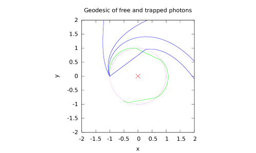
Figure 1: A plot showing photons (null test particles) in the spacetime of a high-flux OR-star with a center at the origin. The dotted circle represents both the (almost degenerate) inner and outer radius of a high flux OR-star. Photons start at the edge of the flat inner radius with various orientations. The blue lines show scattered photons that escape to infinity. The green lines show trapped photon trajectories that repeatedly cross the the OR-star surface in both directions.

This intuition carries over to a relativistic version with a swarm of null particles, each of which follows a bound null geodesic of the spacetime generated by the swarm itself. We call the resulting object an “Orbiting Radiation star” (or OR-star). In this paper, we demonstrate the existence of OR-star solutions to the Einstein equations and discuss their properties. Figure 1 probes an OR-star solution with test-particle photons to illustrate the geometry of the solution.

OR-stars differ quantitatively from but share several qualitative features with the Newtonian scenario above. The relativistic null swarm has both an inner radius $r_{\text{inner}}$ and an outer radius $r_{\text{outer}}$. The inner radius can be of arbitrary real dimension, with a flat spacetime geometry when $r<r_{\text{inner}}$. At the outer radius, which can be significantly larger than the inner radius, the solution matches onto an exterior Schwarzschild geometry. In the OR-star region $r_{\text{inner}}\leq r\leq r_{\text{outer}}$, the null particles follow planar eccentric bound null geodesics arranged in a spherically symmetric configuration. As with most eccentric bound relativistic orbits, these orbits are not simple ellipses, although they do have well-defined pericenters and apocenters at $r_{\text{inner}}$ and $r_{\text{outer}}$, respectively.

To preview some results, the minimum outer radius of an OR-star is 9/8 of its Schwarzschild radius. And, unlike with Schwarzschild black holes, the interior geometry of an OR-star can be probed by observing the deflection pattern and propagation delay of test particle photons sent toward the OR-star.

1.1 Contrast with other solutions

To elucidate some features of OR-stars, it is helpful to contrast them with two other families of solutions to the Einstein equations that exhibit compact objects with deep gravitational wells.

1.1.1 Black holes and similar

The conventional Schwarzschild black hole solution to the Einstein equations has a singularity at the origin and an event horizon at the Schwarzschild radius. Both of these elements ignore the potential for quantum phenomena to modify the solution in the neighborhood of these spacetime regions.

Gravastars [8, 12] are black hole alternatives that rely on Planck length scale effects to resist gravitational collapse. Boson stars [2, 6] rely on low-mass bosons to form compact objects. For particularly large objects, the wavelength of the boson constituents must be particularly large. Related to boson stars are Geons [13]. Spherically symmetric Geons are known to be unstable, since a lower energy configuration exists with two concentric counter-rotating rings  [10]. The timescale of this instability, however, is unclear and almost certainly depends inversely on the size of the object. All of these solutions can be of arbitrary scale, similar to an OR-star, but either rely on quantum effects or ignore them in regimes where quantum effects plausibly matter.

In contrast, OR-stars do not rely on quantum effects or ignore them in regimes where they matter. Its constituents can be any null particle that interacts on large scales only via gravitational effects. These particles can have any energy distribution so long as the energy of any single constituent particle is a negligible fraction of the mass-energy of the entire ensemble. The OR-star has a well-defined continuum limit as an anisotropic but otherwise ideal fluid, as discussed in Section 3.2.

1.1.2 Other null particle solutions

Many null particle solutions to the Einstein equations [1, 4, 5, 7, 11] have been studied. Amongst all these solutions, the scenario of colliding radially ingoing and outgoing null particle streams [4] is a limiting case of the OR-star solution with some substantial technical similarities discussed in Section 7.2.

This solution, however, requires a negative mass at the origin. Although OR-star solutions do also admit a negative central mass and can use that feature to enhance their similarity to Schwarzschild black holes, OR-star solutions do not require exotic negative mass anywhere and in fact can join onto a flat spacetime interior solution. See section 7.2 for details.

1.2 Outline

The rest of this paper is organized as follows. Section 2 lays out preliminaries like coordinate choices and the form of the Einstein tensor for our problem. In Section 3, we derive the stress-energy tensor for an OR-star. In Section 4, we reduce the Einstein equations to a set of coupled ordinary differential equations for the OR-star geometry and for the geodesics of the null particles that comprise it, deferring several computational details to appendices.

In section 5, we discuss various approaches for numerical integration of those equations. We have tried them all and have verified that their results agree within numerical error (we have made all our integration codes available).

In Section 6, we discuss the structure of the solution from several viewpoints. Finally, in Section 7, we discuss variations on the solution family which can be easily handled and their implications.

2 The Einstein tensor

The solution we seek is spherically symmetric and static, so we use radial Schwarzschild coordinates with the following notation for the metric:

$$ds^{2}=-A(r)dt^{2}+B(r)dr^{2}+r^{2}(d\theta^{2}+\sin^{2}(\theta)d\phi^{2})\,.$$ (1)

The metric functions $A(r)$ and $B(r)$ should match onto their Schwarzschild values at the outer edge $r=r_{\text{outer}}$ of the OR-star.

Because an OR-star is made up of null particles, its total stress-energy tensor will be traceless (see equations (37)–(39)). The Einstein tensor must therefore also be traceless, which implies that the Ricci scalar vanishes identically. As a result, just as in vacuum spacetimes, the Einstein tensor in an OR-star spacetime is simply the Ricci tensor, which in these coordinates has nonvanishing components

$$R_{tt} = \frac{A^{\prime\prime}}{2B}+\frac{A^{\prime}}{rB}-\frac{A^{\prime}}{4B}\left(\frac{A^{\prime}}{A}+\frac{B^{\prime}}{B}\right)$$ (2a)

$$R_{rr} = -\frac{A^{\prime\prime}}{2A}+\frac{B^{\prime}}{rB}+\frac{A^{\prime}}{4A}\left(\frac{A^{\prime}}{A}+\frac{B^{\prime}}{B}\right)$$ (2b)

$$R_{\theta\theta} = 1-\frac{1}{B}-\frac{r}{2B}\left(\frac{A^{\prime}}{A}-\frac{B^{\prime}}{B}\right)$$ (2c)

$$R_{\phi\phi} = \sin^{2}(\theta)R_{\theta\theta}$$ (2d)

3 The stress-energy tensor

The particles comprising an OR-star follow null geodesics of the spacetime generated by those same null particles. A description of those null geodesics allows us to deduce the form of the stress-energy tensor of the entire OR star. When all those geodesics have the same magnitude impact parameter $\lvert b\rvert$ and are distributed in a spherically symmetric way, the resulting OR-star can be interpreted as an anisotropic fluid with a distinct radial and tangential pressure at every point.

3.1 Null geodesics of OR-star particles

We derive the equations of motion along the fiducial null geodesic of a single OR-star particle. The trajectory and 4-velocity of any other particle can be derived from this fiducial geodesic by some combination of rotation within the orbital plane, rotation of the orbital plane, and a translation of orbital phase.

Spherical symmetry lets us choose the equatorial plane $\theta\equiv\pi/2$ to be the orbital plane of the fiducial geodesic without loss of generality. $\partial_{\phi}$ is then a Killing vector, so a particle with 4-momentum $p^{\mu}$ has a conserved angular momentum

$$L\equiv g_{\mu\nu}\partial_{\phi}^{\mu}p^{\nu}$$ (3)

that we allow to take any sign. Because it is static, an OR-star spacetime also has a timelike Killing vector $\partial_{t}$ that yields a conserved “energy at infinity”

$$E^{\infty}\equiv-g_{\mu\nu}\partial_{t}^{\mu}p^{\nu}\,.$$ (4)

We define the impact parameter of each particle to be

$${\color[rgb]{1,0,0}b}\equiv\frac{L}{E^{\infty}}$$ (5)

and allow it to take any sign (matching the sign of $L$ and $\dot{\phi}$). Because two null particles with the same ${\color[rgb]{1,0,0}b}$ but different energies still follow the same geodesic, it is useful to define an affine parameter $\lambda$ along null geodesics

$$\frac{dx^{\mu}}{d\lambda}\equiv u^{\mu}\equiv\dot{x}^{\mu}\equiv\frac{1}{E^{\infty}}p^{\mu}$$ (6)

that absorbs this energy factor so that it need not appear explicitly in the equations of motion.

Equation (4) then yields the equation for $\dot{t}$,

$$E^{\infty}=-(-A(r))E^{\infty}\dot{t}\longrightarrow\dot{t}=\frac{1}{A(r)}\,,$$ (7)

while (3) yields $\dot{\phi}$,

$$L=r^{2}E^{\infty}\dot{\phi}\longrightarrow\dot{\phi}=\frac{b}{r^{2}}\,.$$ (8)

For the fiducial geodesic, $\dot{\theta}\equiv 0$ by our choice of equatorial plane. Finally, the radial equation of motion follows from the fact that the 4-velocity $u^{\mu}$ of OR-star particles is null. Using (7) and (8) to eliminate $\dot{t}$ and $\dot{\phi}$, we get

$$0=g_{\mu\nu}u^{\mu}u^{\nu} =-A\dot{t}^{2}+B\dot{r}^{2}+r^{2}\dot{\theta}^{2}+r^{2}\sin^{2}(\theta\equiv\frac{\pi}{2})\dot{\phi}^{2}$$ (9)

$$=-\frac{1}{A}+B\dot{r}^{2}+\frac{{\color[rgb]{1,0,0}b}^{2}}{r^{2}}$$ (10)

$$\longrightarrow\dot{r}^{2} =\frac{1}{AB}\left(1-\frac{A{\color[rgb]{1,0,0}b}^{2}}{r^{2}}\right)$$ (11)

$$\longrightarrow\dot{r} =\pm\frac{1}{\sqrt{AB}}\left(1-\frac{Ab^{2}}{r^{2}}\right)^{1/2}\,.$$ (12)

Thus the 4-velocity of our fiducial null geodesic is

$$u^{\mu}(t,r,\theta,\phi)=\left[\begin{array}[]{c}1/A\\ \pm\sqrt{\frac{1}{AB}}\sqrt{1-\frac{A{\color[rgb]{1,0,0}b}^{2}}{r^{2}}}\\ 0\\ \frac{{\color[rgb]{1,0,0}b}}{\sin(\theta)r^{2}}\end{array}\right]=\frac{1}{A}\left[\begin{array}[]{c}1\\ \pm\sqrt{\frac{A}{B}}\sqrt{1-\frac{A{\color[rgb]{1,0,0}b}^{2}}{r^{2}}}\\ 0\\ \frac{A{\color[rgb]{1,0,0}b}}{r^{2}\sin(\theta)}\end{array}\right]\,.$$ (21)

More generally, if the spatial velocity of an OR-star particle at $r$ makes an angle $\gamma$ when projected onto the sphere of radius $r$, then its 4-velocity is (where $\gamma=0$ would be latitudinal and $\gamma=\pi/2$ would be longitudinal)

$$u^{\mu}(t,r,\theta,\phi;\gamma)=\frac{1}{A}\left[\begin{array}[]{c}1\\ \pm\sqrt{\frac{A}{B}}\sqrt{1-\frac{A{\color[rgb]{1,0,0}b}^{2}}{r^{2}}}\\ \sin(\gamma)\frac{A{\color[rgb]{1,0,0}b}}{r^{2}}\\ \cos(\gamma)\frac{A{\color[rgb]{1,0,0}b}}{\sin(\theta)r^{2}}\end{array}\right]=\frac{1}{A}\left[\begin{array}[]{c}1\\ {}\hfil\\ \vec{v}\\ {}\hfil\end{array}\right]\,,$$ (30)

with $\vec{v}$ denoting the ordinary spatial velocity 3-vector in the standard Schwarzschild coordinate basis.

3.2 OR-stars as anisotropic fluids

The stress-energy tensor for the entire OR-star should be the sum of the individual stress-energy tensors of all the constituent null particles. $T^{\mu\nu}$ for a single null particle with 4-velocity $u$ is essentially that of a null dust

$$T\sim\rho u\otimes u$$ (31)

with delta functions as appropriate in the energy density $\rho$.

Consider a local orthonormal frame field with basis vectors and basis one-forms

$$e_{\hat{t}} =\frac{1}{\sqrt{A(r)}}\partial_{t} \quad de^{\hat{t}} =-\sqrt{A(r)}dt$$

$$e_{\hat{r}} =\frac{1}{\sqrt{B(r)}}\partial_{r} \quad de^{\hat{r}} =\sqrt{B(r)}dr$$

$$e_{\hat{\theta}} =\frac{1}{r}\partial_{\theta} \quad de^{\hat{\theta}} =rd\theta$$

$$e_{\hat{\phi}} =\frac{1}{r\sin\theta}\partial_{\phi} \quad de^{\hat{\phi}} =r\sin\theta d\phi\,.$$ (32)

Since all the particles have the same impact parameter magnitude $\lvert{\color[rgb]{1,0,0}b}\rvert$, the $\vec{v}$ distribution in a local orthonormal frame is anisotropic. The projection $v^{\perp}$ of $\vec{v}$ into the spatial plane normal to $e_{\hat{r}}$ is isotropic within that plane, so that

$$\langle(v^{\hat{\theta}})^{2}\rangle=\langle(v^{\hat{\phi}})^{2}\rangle=\frac{1}{2}\langle(v^{\perp})^{2}\rangle\,.$$ (33)

But, as we can see from (30) and (3.2), the angle between $v^{\hat{r}}$ and $v^{\perp}$ varies with $r$, so that in general,

$$\langle(v^{\hat{r}})^{2}\rangle\equiv 1-\langle(v^{\perp})^{2}\rangle\neq\frac{1}{2}\langle(v^{\perp})^{2}\rangle\,.$$ (34)

Thus, the radial pressure

$$P_{r}=\rho\langle(v^{\hat{r}})^{2}\rangle$$ (35)

and the tangential pressure

$$P_{\theta}=P_{\phi}=\frac{1}{2}\rho\langle(v^{\perp})^{2}\rangle\equiv P_{\perp}$$ (36)

are unequal in general.

Taking the continuum limit, an OR-star is an anistropic fluid whose stress-energy tensor in the local orthonormal rest frame of a fluid element is

$$T^{\hat{\mu}\hat{\nu}}=\text{diag}(\rho,P_{r},P_{\perp},P_{\perp})\,,$$ (37)

or, in manifestly covariant form (see, e.g., [9] or [4]),

$$T^{\mu\nu}=(\rho+P_{\perp})u^{\mu}u^{\nu}+P_{\perp}g^{\mu\nu}+(P_{r}-P_{\perp})e_{\hat{r}}^{\mu}e_{\hat{r}}^{\nu}\,.$$ (38)

Even though the fluid consists of null particles, each resulting fluid element has a timelike 4-velocity $u^{\mu}$ and a well-defined rest frame. However, because the OR-star consists of null particles, we still expect this $T^{\mu\nu}$ to be traceless. And it is – the speed of light is unity in all local Lorentz frames, so from (35) and (36, we get

$$P_{r}+2P_{\perp}=\rho(\langle(v^{r})^{2}\rangle+\langle(v^{\perp})^{2}\rangle=\rho\,.$$ (39)

3.3 Explicit expression for $T_{\mu\nu}$

To conclude this section, we derive an explicit expression for the stress-energy tensor (38) in terms of $r$, the (still unknown) metric coefficient functions $A(r)$ and $B(r)$, and a small number of parameters that characterize an OR-star.

Let $n_{+}(r)$ and $n_{-}(r)$ denote the number densities at $r$ (as measured in frame (3.2)) of null particles with $v^{\hat{r}}>0$ (outward bound) and $v^{\hat{r}}<0$ (inward bound), respectively. $n_{+}(r)$ must equal $n_{-}(r)$ at every $r$ – if, say, $n_{+}$ were larger, then when the radial velocities of all the particles changed sign after half a radial period of the null geodesics, $n_{-}$ would be larger, counter to the assumption of staticity.

As measured in frame (3.2), the radial component of the spatial velocity $\vec{v}$ for null particles moving radially outward ($v^{\hat{r}}>0$)across the spherical surface at $r$ is (using (30) and (3.2))

$$v^{\hat{r}}\equiv d\hat{r}/d\hat{t} =\frac{\sqrt{B}}{\sqrt{A}}\frac{dr}{dt}$$ (40)

$$=\frac{\sqrt{B}}{\sqrt{A}}\frac{\sqrt{A}}{\sqrt{B}}\sqrt{1-\frac{A{\color[rgb]{1,0,0}b}^{2}}{r^{2}}}$$ (41)

$$=\sqrt{1-\frac{A{\color[rgb]{1,0,0}b}^{2}}{r^{2}}}\,.$$ (42)

In the local orthonormal frame (3.2), these radially outward-bound particles cross the spherical surface at $r$ at a rate

$$\frac{dN}{d\hat{t}} =n_{+}(r)4\pi r^{2}v^{\hat{r}}$$ (43)

$$=n_{+}(r)4\pi r^{2}\sqrt{1-\frac{A{\color[rgb]{1,0,0}b}^{2}}{r^{2}}}\,,$$ (44)

where $n_{+}(r)$ denotes the (also locally measured) number density of outward flowing particles. Because the system must be time-reversal invariant, we must have

$$n_{+}(r)\equiv n_{-}(r)\equiv\frac{1}{2}n(r)\,,$$ (45)

where $n(r)$ is the total local particle number density (outbound and inbound).

In terms of the Schwarzschild time coordinate $t$, the rate corresponding to (43) is time-dilated to

$$\frac{dN_{+}}{dt} =\sqrt{A}\frac{dN_{+}}{d\hat{t}}$$ (46)

$$=\sqrt{A}n_{+}(r)4\pi r^{2}v^{\hat{r}}$$ (47)

$$=\sqrt{A}\frac{1}{2}n(r)4\pi r^{2}\sqrt{1-\frac{A{\color[rgb]{1,0,0}b}^{2}}{r^{2}}}\,.$$ (48)

By staticity, this rate must be independent of $t$. It must also be independent of $r$ – after one coordinate radial period $T_{r}$ of the geodesics, every particle returns with the same velocity to the spherical surface from which it departed, and the “geodesic conveyor belt” has carried every particle in the OR-star outward across the spherical surface at $r$ exactly once. Therefore, if the total number of particles in the OR-star is $N$, then

$$2\pi\sqrt{A(r)}n(r)r^{2}\sqrt{1-\frac{A(r){\color[rgb]{1,0,0}b}^{2}}{r^{2}}}\equiv\frac{N}{T_{r}}\,,$$ (49)

and the local particle number density is

$$n(r)=\frac{N/T_{r}}{2\pi}\frac{1}{\sqrt{A(r)}r^{2}\sqrt{1-\frac{A(r){\color[rgb]{1,0,0}b}^{2}}{r^{2}}}}\,.$$ (50)

Now multiply both sides of (50) by the average particle energy in the local frame $\langle E^{\text{loc}}\rangle=\langle E^{\infty}\rangle/\sqrt{A(r)}$. On the LHS, we get the local energy density

$$\rho(r)\equiv n(r)\langle E^{\text{loc}}\rangle(r)$$ (51)

that appears in (38). On the RHS, we get

$$\phantom{=}\frac{\langle E^{\infty}\rangle N/T_{r}}{2\pi}\frac{1}{\sqrt{A(r)}}\frac{1}{\sqrt{A(r)}r^{2}\sqrt{1-\frac{A(r){\color[rgb]{1,0,0}b}^{2}}{r^{2}}}}$$ (52)

$$=\frac{M_{\text{OR}}/T_{r}}{2\pi}\frac{1}{A(r)r^{2}\sqrt{1-\frac{A(r){\color[rgb]{1,0,0}b}^{2}}{r^{2}}}}\,,$$ (53)

where $M_{\text{OR}}$ is the total mass of the OR-star measured by distant observers, and $M_{\text{OR}}/T_{r}$ is the “energy circulation rate” of particles within the OR-star.

We absorb all the prefactors into a single constant

$${\color[rgb]{1,0,0}\tilde{m}}\equiv\frac{M_{\text{OR}}/T_{r}}{2\pi}$$ (54)

and define a convenience function

$$m(r)\equiv\frac{{\color[rgb]{1,0,0}\tilde{m}}}{r^{2}\sqrt{1-b^{2}A(r)/r^{2}}}\,.$$ (55)

The local energy density in the OR-star is then

$$\rho(r)=\frac{{\color[rgb]{1,0,0}\tilde{m}}}{A(r)r^{2}\sqrt{1-\frac{A(r){\color[rgb]{1,0,0}b}^{2}}{r^{2}}}}=\frac{m(r)}{A(r)}\,.$$ (56)

Using (56), (35), (36) and (30), the pressures $P_{r}(r)$ and $P_{\perp}(r)$ can also be expressed in terms of $r,A,B,m(r)$ and ${\color[rgb]{1,0,0}b}$.

Combining those results with the metric (1) and equation (38), we arrive at the following expression for the nonvanishing components (in the Schwarzschild coordinate basis) of the OR-star stress-energy tensor

$$T^{tt} = {\color[rgb]{0,0,1}m}(r)/A^{2}$$ (57a)

$$T^{rr} = \frac{{\color[rgb]{0,0,1}m}(r)}{AB}(1-A{\color[rgb]{1,0,0}b}^{2}/r^{2})$$ (57b)

$$T^{\theta\theta} = {\color[rgb]{0,0,1}m}(r){\color[rgb]{1,0,0}b}^{2}/(2r^{4})$$ (57c)

$$T^{\phi\phi} = T^{\theta\theta}/\sin^{2}(\theta)\,.$$ (57d)

The $(0,2)$ version of the tensor $T_{\mu\nu}=g_{\alpha\mu}g_{\beta\nu}T^{\alpha\beta}$ is

$$T_{tt} = {\color[rgb]{0,0,1}m}(r)$$ (58a)

$$T_{rr} = \frac{{\color[rgb]{0,0,1}m}(r)B}{A}(1-A{\color[rgb]{1,0,0}b}^{2}/r^{2})$$ (58b)

$$T_{\theta\theta} = {\color[rgb]{0,0,1}m}(r){\color[rgb]{1,0,0}b}^{2}/2$$ (58c)

$$T_{\phi\phi} = T_{\theta\theta}\sin^{2}(\theta)\,.$$ (58d)

Note that an OR-star is specified by two parameters in terms of which all other parameters are determined: ${\color[rgb]{1,0,0}\tilde{m}}$ (the energy circulation rate in the OR-star, which we will sometimes refer to simply as “the flux”), and ${\color[rgb]{1,0,0}b}^{2}$ (the square of the impact parameter). The total mass of the OR-star is also a parameter, but adjusting it merely rescales any given solution (see section 4.2).

4 The Einstein equations for an OR-star

4.1 Derivation of ODEs

As discussed in Section 2, the Einstein equations for an OR-star become

$$R_{\mu\nu}=8\pi GT_{\mu\nu}\,,$$ (59)

with the left- and right-hand sides, respectively, defined by (2) and (58). As we demonstrate in the Appendix, the fact that

$$\operatorname{tr}T\equiv T^{\mu}_{\phantom{\mu}\mu}=0\,$$ (60)

helps us reduce (59) to a pair of coupled, nonlinear 1st-order ODEs for the metric coefficients $A(r)$ and $B(r)$,

$$rA^{\prime}/A = \frac{{\color[rgb]{1,0,0}\tilde{m}}B\sqrt{1-{\color[rgb]{1,0,0}b}^{2}A/r^{2}}}{A}+B-1$$ (61a)

$$rB^{\prime}/B = \frac{{\color[rgb]{1,0,0}\tilde{m}}B}{A\sqrt{1-{\color[rgb]{1,0,0}b}^{2}A/r^{2}}}-B+1\,,$$ (61b)

where a prime denotes differentiation with respect to $r$.

To prove the above, we develop an equation for $rA^{\prime}/A$ and $rB^{\prime}/B$ which holds for all null particle problems. In other words, only under the assumption that $T=g_{\alpha\alpha}T^{\alpha\alpha}=0$, we can get some simplifications of the Einstein equations. In particular, we eliminate the $A^{\prime\prime}$ from our equations for $R_{tt}$ and $R_{rr}$.

Lemma 1.

If $g_{\nu\nu}T^{\nu\nu}=0$, we can write our ODE in terms of $T$’s:

$$A^{\prime}/A = -16\pi GBr^{3}T^{\theta\theta}+8\pi GrBAT^{tt}+B/r-1/r$$ (62)

$$B^{\prime}/B = 8\pi GrBAT^{tt}-B/r+1/r$$ (63)

The proof is in the appendix.

Proof of equations (61a) and (61b): From equations 57a,57d, and (55) we get:

$$T^{tt} = {\color[rgb]{0,0,1}m}/A^{2}$$

$$T^{\theta\theta} = {\color[rgb]{0,0,1}m}{\color[rgb]{1,0,0}b}^{2}/(2r^{4})$$

Plugging these in to lemma 1 we get:

$$A^{\prime}/A = -16\pi GBr^{3}{\color[rgb]{0,0,1}m}{\color[rgb]{1,0,0}b}^{2}/(2r^{4})+8\pi GrBA{\color[rgb]{0,0,1}m}/A^{2}+B/r-1/r$$

$$B^{\prime}/B = 8\pi GrBA{\color[rgb]{0,0,1}m}/A^{2}-B/r+1/r$$

which simplifies as:

$$A^{\prime}/A = -8\pi GB{\color[rgb]{0,0,1}m}{\color[rgb]{1,0,0}b}^{2}/r+8\pi GrB{\color[rgb]{0,0,1}m}/A+B/r-1/r$$

$$B^{\prime}/B = 8\pi GrB{\color[rgb]{0,0,1}m}/A-B/r+1/r$$

Now plugging in ${\color[rgb]{0,0,1}m}$ from equation 55 and setting ${\color[rgb]{1,0,0}\hat{m}}=8\pi G{\color[rgb]{1,0,0}\tilde{m}}$ we get:

$$A^{\prime}/A = {\color[rgb]{1,0,0}\hat{m}}\frac{rB/A-B{\color[rgb]{1,0,0}b}^{2}/r}{r^{2}\sqrt{1-{\color[rgb]{1,0,0}b}^{2}A/r^{2}}}+B/r-1/r$$

$$B^{\prime}/B = \frac{{\color[rgb]{1,0,0}\hat{m}}B}{rA\sqrt{1-{\color[rgb]{1,0,0}b}^{2}A/r^{2}}}-B/r+1/r$$

which is

$$A^{\prime}/A = {\color[rgb]{1,0,0}\hat{m}}(Br/A)\frac{1-{\color[rgb]{1,0,0}b}^{2}A/r^{2}}{r^{2}\sqrt{1-{\color[rgb]{1,0,0}b}^{2}A/r^{2}}}+B/r-1/r$$

$$B^{\prime}/B = \frac{{\color[rgb]{1,0,0}\hat{m}}B}{rA\sqrt{1-{\color[rgb]{1,0,0}b}^{2}A/r^{2}}}-B/r+1/r$$

and simplifies to

$$A^{\prime}/A = \frac{{\color[rgb]{1,0,0}\hat{m}}B\sqrt{1-{\color[rgb]{1,0,0}b}^{2}A/r^{2}}}{Ar}+B/r-1/r$$

$$B^{\prime}/B = \frac{{\color[rgb]{1,0,0}\hat{m}}B}{rA\sqrt{1-{\color[rgb]{1,0,0}b}^{2}A/r^{2}}}-B/r+1/r.$$

Multiplying by $r$ completes the proof. $\Box$

4.2 The solution family

All OR-star solutions have an inner radius and an outer radius. The inner radius $r_{\text{inner}}$ is the smallest radius that constituent null particles achieve while the outer radius $r_{\text{outer}}$ is the largest radius that constituent null particles achieve.

Other key parameters are the flux ${\color[rgb]{1,0,0}\tilde{m}}$, the impact parameter ${\color[rgb]{1,0,0}b}$, and the boundary conditions for $A$ and $B$. Using symmetries and dependencies, we reduce this to a one-dimensional family of solutions. To see this, we first describe two invariances of the ODEs.

1. If $A$, and $B$ are solutions for (61a) and (61b) with parameters ${\color[rgb]{1,0,0}b}$ and ${\color[rgb]{1,0,0}\tilde{m}}$, then for any constant $k$, $kA$ and $B$ are solutions for ${\color[rgb]{1,0,0}b}/\sqrt{k}$ and $k{\color[rgb]{1,0,0}\tilde{m}}$.

   $$A(r),B(r)\hbox{ satisfy (\ref{eqn:dean:A})-(\ref{eqn:dean:B})}\Longrightarrow kA(r),B(r)\hbox{ satisfy (\ref{eqn:dean:A})-(\ref{eqn:dean:B})}$$ (64)

   We use this property in our simulations to set $A(r_{\text{inner}})=1$. After the fact, this symmetry can be used to set $A(\infty)=1$ as per convention.

2. If $A(r)$ and $B(r)$ are solutions (61a) and (61b) with parameters ${\color[rgb]{1,0,0}b}$ and ${\color[rgb]{1,0,0}\tilde{m}}$, then for any constant $k$, $A(kr)$ and $B(kr)$ are solutions for $k{\color[rgb]{1,0,0}b}$ and $k{\color[rgb]{1,0,0}\tilde{m}}$.

   $$A(r),B(r)\hbox{ satisfy (\ref{eqn:dean:A})-(\ref{eqn:dean:B})}\Longrightarrow A(kr),B(kr)\hbox{ satisfy (\ref{eqn:dean:A})-(\ref{eqn:dean:B})}$$ (65)

   This scale invariance implies we can set $r_{\text{inner}}=1$ in our simulations.

A few other simplifications are immediate.

1. We have $B(r_{\text{inner}})=1$ since we are seeking a solution which is flat inside the inner radius. As long as the mass distribution is compact, this implies $B(\infty)=1$ as well.

2. Since $A(r_{\text{inner}})=1$ and $r_{\text{inner}}=1$, we must have $b=1$.

3. Given $A(r_{\text{inner}})=1$, $B(r_{\text{inner}})=1$, $r_{\text{inner}}=1$, and the flux ${\color[rgb]{1,0,0}\tilde{m}}$, the value of $r_{\text{outer}}$ is determined.

The remaining free parameter is the flux ${\color[rgb]{1,0,0}\tilde{m}}$ which indexes the family of solutions.

Semi-analytic solutions

There are three special cases which can be approximated analytically. The first is low flux. Since low flux implies low curvature, photons starting at the inner radius move almost directly away from the center at large $r$. So for large $r$, it is basically a counter flux of inward photons and outward photons. Hence the solution of Gergely [4] is a good approximation. We can define ${\color[rgb]{1,0,0}\tilde{m}}_{0}$ as the maximum flux for which a closed OR-star is not formed.

A second analytic solution arises in the close-to-critical case. Here there is just barely enough intensity to close the “orbits.” In this case, the photons end up spiraling to and away from the outer radius with their radius changing infinitesimally, limiting to a perfect circle. The following theorem applies with proof in the Appendix.

Theorem 1.

If ${\color[rgb]{1,0,0}b}=1$ and ${\color[rgb]{1,0,0}\tilde{m}}$ close to ${\color[rgb]{1,0,0}\tilde{m}}_{0}$, then $B(r)\approx 3$ and $A(r)\approx r^{2}$ is a solution to our equations. In particular,

$$A/r^{2} = 1-9{\color[rgb]{1,0,0}\tilde{m}}^{2}r^{-4}/4+O({\color[rgb]{1,0,0}\tilde{m}}^{6}r^{-12})$$ (66)

$$B = 3+9{\color[rgb]{1,0,0}\tilde{m}}^{2}r^{-4}/2+O({\color[rgb]{1,0,0}\tilde{m}}^{4}r^{-8})$$ (67)

A third analytic solution arises in the high-flux case. If the flux is high enough, then the inner and outer radius are almost the same. Hence there is basically no dependence on $r$ in the ODEs and they can be solved exactly. The following theorem applies with proof in the Appendix.

Theorem 2.

For high flux (i.e. ${\color[rgb]{1,0,0}\tilde{m}}\approx\infty$), the maximum achievable value for $B$ is $B\approx 9$, with $r_{\text{inner}}\simeq r_{\text{outer}}\simeq 2.25$.

From these two theorems, we can catalog OR-stars by the maximal value that $B$ ever obtains. If $B_{max}<3$, then the OR-star must be open and the photons never return. If $3\leq B_{max}\leq 9$ then the OR-star is closed with a flat interior. There are no OR-stars with a flat interior spacetime that have $B_{\text{max}}>9$.

5 Methods of Integration and Simulation

Given the partial differential equations from the previous section, there are several ways to do an integration (or simulation) to discover the geometry of the object. We tried two in order to convince ourselves that the results are sound. Both approaches can be easily implemented on a desktop computer and run fairly quickly.

5.1 Integrating Differential Equations

At $r_{\text{inner}}$ and $r_{\text{outer}}$, where the spatial velocity of the null particles is instantaneously parallel to the inner and outer spherical surfaces of the OR-star, the density diverges to infinity like $\rho(r)\sim 1/\sqrt{r-r_{\text{inner/outer}}}$. But this density still integrates to a finite value, so that the total mass can be well-approximated numerically by integrating very close to $r_{\text{inner}}$ and $r_{\text{outer}}$. We tested this approach using the deSolve package in R which uses Runge-Kutta techniques for integration.

5.2 Integration from the inner radius to the outer radius

To confirm that we are not losing essential physics near the inner and outer radius, we also tried an alternative numerical approach, using as the integration variable the affine parameter of an element of null particles traveling from $r_{\text{inner}}$ to $r_{\text{outer}}$.

In essence, this approach does integration-by-simulation. Since spherical symmetry exists, we can pick any element at the inner radius and follow its trajectory to the outer radius, referring to the element’s radius to index a differential shell of elements of two sorts:

1. Elements starting simultaneously on the inner radius with positions uniform on the inner sphere and trajectories drawn from uniform tangents to the inner sphere.

2. Elements of the same mass/energy at the same radius returning from a hypothesized outer radius. Conservation principles imply that such elements must have the same mass/energy as elements of the first sort differing only in the sign of their radial velocity.

This simulation is self-consistent if the curvature generated creates an outer radius where the geodesic has no radial component. At this point, the simulation can halt because we have already accounted for the contribution of elements returning from the outer radius to the inner radius.

In more detail, we can start the simulation with $r=1,A(1)=1,B(1)=1$ at the inner radius and a free parameter given by ${\color[rgb]{1,0,0}\tilde{m}}$ as discussed in section 4.2. Furthermore, the null particle must be tangential to the inner radius, implying ${\color[rgb]{1,0,0}b}=1$.

If we let $\delta$ be the simulation scale, the equations for the forward step then become (after some algebra):

1. $m\leftarrow r\frac{B-1}{2B}$ //the mass inside the radius

2. $dm\leftarrow\delta\frac{4\pi{\color[rgb]{1,0,0}\tilde{m}}\sqrt{r-2m}}{r^{1/2}A^{3/2}}$ //the change in mass

3. $\phi\leftarrow\frac{1}{2}\ln(A)$//the current angle of null particle

4. $d\phi\leftarrow\delta\frac{Am+4\pi{\color[rgb]{1,0,0}\tilde{m}}\sqrt{r^{2}-A}}{r^{3}A^{3/2}}$//the change in angle

5. $dr\leftarrow\delta\frac{\sqrt{r^{2}-A}}{r\sqrt{AB}}$//the change in radius

This leads to new values according to:

1. $r\leftarrow r+dr$

2. $m\leftarrow m+dm$

3. $B\leftarrow\frac{r}{r-2m}$

4. $\phi\leftarrow\phi+d\phi$

5. $A\leftarrow e^{2\phi}$

We can record the values of $r,A,B$ and simulate forward to the outer radius. With a self-consistent solution for the shell, attaching a Schwarzschild geometry onto the outer radius provides a solution everywhere. Then $A(r)$ can be rescaled so $A(r)=1$ in the asymptotic rest frame.

We implemented this integration/simulator using C++ doing simple first-order integration according to Euler’s method (as above). The results are quantitatively stable to high precision and agree with the Runge-Kutta approach. Our code is available [3].

5.3 Ray Tracing

In order to test our understanding of the OR-star object, we also created a four-dimensional ray-tracer to probe the family of geodesics that test-particle photons traverse . This process is a simple computation given the geometry $A(r)$ and $B(r)$ and conservation of angular momentum.

To do this efficiently, we recorded the geometry at each discrete radius given by the integration/simulation above and used a simple linear interpolation between the two nearest recorded points.

Searching for the geometry can be done for a point at an arbitrary radius by first testing whether the radius is within the shell of the object. If it’s interior, the geometry is flat. If it’s exterior, then the geometry is Schwarzschild. If it’s in the shell, then a binary search suffices, although a hinted location reduces this search to amortized constant time in the case of ray tracing.

6 Simulation results

We exercised our simulations in various ways to both check correctness and understand the implications of OR-stars.

An important concept is the characteristic geodesic. A characteristic geodesic is the path that null particles takes when starting tangential to the inner radius at the inner radius. When this is gravitationally closed, the characteristic geodesic can be glued together from inner radius to outer to inner to outer etc… to get the path of null particles.

6.1 Varying initial conditions

Here we exercise initial conditions to get a sense of the solution structure.

6.1.1 Varying radius

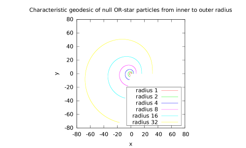
Figure 2: A plot of the characteristic geodesic from inner to outer radius for OR-stars with varying radius but the same flux. This graphically shows (65).

Figure 2 shows the structure of the characteristic geodesic is invariant to the radius, implying that the scale of the structure can be arbitrary, as expected.

6.1.2 Low mass/energy flux

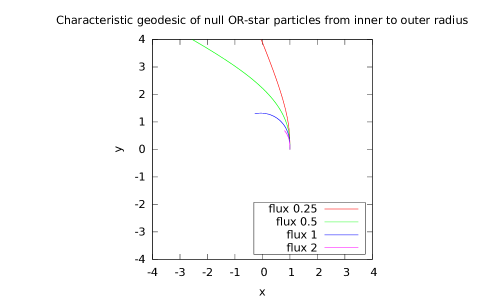
Figure 3: The characteristic geodesic for OR-stars with the same inner radius but different flux.

Figure 4: An “open” OR-star with insufficient null particles for a compact object. The upper plot shows $A$ with a yellow background showing the region of null particles. The lower plot shows the value of $B$ and the density of the mass.

In Figure 3 we see that the structure of the characteristic geodesic as the mass/energy flux varies. This result has more structure, because the results with 0.25 or 0.5 flux are not closed.

This result is as expected—low amounts of mass/energy should not be able to generate sufficient curvature for geodesics to curl back.

In Figure 4 we show the time geometry $A=g_{tt}$ and radial geometry $B=g_{rr}$. The difference between our model and colliding null particles [4] is that colliding null particles head directly towards or away from the center—an impact parameter of zero. Making this works requires a negative mass singularity at the origin. We avoid this with null particles having a greater impact parameter, generating an inner radius of closest approach. At a few multiples of the inner radius from origin, the photons head almost exactly away from the origin so the equations are similar to the colliding null particles solution.

For such an open object, the maximal value of $B$ is always less than 3–namely the $B$ corresponding to the photon sphere. The open object with the largest $B$ has null particles orbiting in a photon sphere at each possible radius.

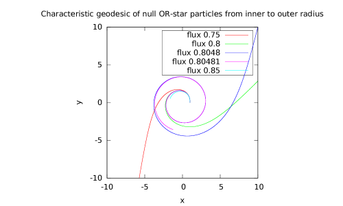
Figure 5: A plot of the characteristic geodesic from inner to outer radius for OR-stars with the same inner radius but varying flux near the critical flux. Geodesics reaching the edge of the plot do not close.

6.1.3 The critical mass/energy flux

In Figure 5 we see variations around the critical point where curvature becomes sufficient to create closed geodesics. In this plot, all non-closed geodesics reach the graph edge and are valid when the null particles are reflected towards the origin.

Figure 6 shows $A$, $B$, and the potential well created by a near-critical closed solution. $B$ just barely increases past $3$ and the null particles returns towards zero. Near-critical closed solutions are unstable since photons significantly off the characteristic curve escape to infinity.

6.1.4 High mass/energy flux

Figure 6: This is a near critical OR-star. The upper plot shows $A$ with a yellow background showing the region with null particles. The lower plot shows the value of $B$ and the density.

The final example in this section is a high flux version (see figure 7). The maximal $B=1/(1-2/2.25)=2.25/.25=9$ matches the bound in Theorem 2 for the maximal mass which doesn’t collapse into a black hole. This is a much more stable object as illustrated by the trapped photons of Figure 1 in the introduction.

Figure 7: This is a high flux OR-star. The upper plot shows $A$ with a yellow background showing the region with null particles. The lower plot shows the value of $B$ and the density.

6.2 Observational differences from a black hole

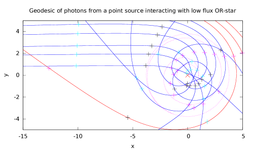
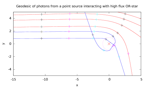
Figure 8: Geodesics as traced by photons from a point source far to the left interacting with a near-critical OR-star (above) and high flux OR-star (below) at the origin. The origin is marked in red, and the structure of the OR-star (inner radius, outer radius, and characteristic geodesic) are shown with dotted lines. For the high flux OR-star these overlap leaving only a circle. The black, red, and light blue tics mark equal separation in time as measured by the point source. The red lines are Schwarzschild geodesics while the blue lines are not.

The structure of the object is similar to but observationally different from a black hole because geodesics from infinity can probe the geometry at all points and return to infinity. In Figure 8 we show the geodesics traced by photons from a point source far away. The expected external structure of Schwarzschild geometry is observed, but the internal structure is substantially more complicated. It’s easy to observe that the tics of coordinate time advance more slowly in the interior from the viewpoint of an observer far from the object, as expected.

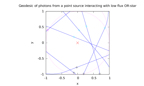
Figure 9: A zoom on the same plot as figure 8 showing that the focal point is imperfect and the internal space is flat as expected.

In Figure 9 we zoom in to see the internal structure in the flat internal region. As expected, the geodesics are all straight lines in this region, although it is interesting to notice that the geodesics all focus on a point. The focal point is well within the inner radius and clearly imperfect.

Considering the global structure again, the object differs from a black hole observationally for any geodesic crossing the outer radius. Every photon crossing the outer radius is less tangential than the null particles composing the OR-star. This monotonicity property is preserved as the photon and null particles travel to the inner radius where the photon must therefore enter the inner radius since it is not tangential.

Photons aimed directly at the center have their coordinate time retarded by the mass of the object but are otherwise unaltered as observed asymptotically. Hence, the object acts as a “timescope” allowing an observer to record what happened on the other side of the object in the past.

One observational signature of the OR-star for a stationary observer is therefore a combination of normal gravitational lensing via Schwarzschild geodesics plus a time delayed observation of a point source. When the point source and the observer are moving relative to the OR-star, it is still possible to observe a signature, because there often exists a geodesic between the point source and the observer passing through the object. Observation of the geodesic passing through the object is difficult because small changes in input angle from the source result in large changes in the required angle of an observer. In essence, an OR-star  lights up for observers at many angles with only a small solid angle of input photons. Since the small angle of input photons are shared by many observers, it is relatively dim.

Hence, a second signature of an OR-star is given by widely dispersed observers that record a dim version of the same time-delayed event nearby to the object. On such possibility would be given by a nearby star that novas. First, observers would see nova via Schwarzschild geodesics, and then a dim time-delayed “echo” of the nova event via non-Schwarzschild geodesics passing through the OR-star.

7 Solution Variations

Several variations on the object are straightforward given the above. We discuss them here for further consideration.

7.1 Mass inside the inner radius

Up to this point we have been using a flat geometry inside the inner shell, but other spherically symmetric inner geometries can be handled as long as geodesics starting on the inner sphere increase in radius. The only modification to the inner solution is an increased amount of time dilation which can be determined after the fact as per our existing simulation/solution. The calculation of the characteristic geodesic and the geometry between the inner and outer shell is only modified by a change to the initial conditions in the inside-outside simulation approach. In essence, instead of starting with a mass of $0$, you start with the mass of the inner solution using the geometry that this implies.

7.2 An OR-star with a (near) event horizon

If the inner contains flat space, then the smallest outer radius for a mass 1 object is $2.25$ and the maximum value of $B$ is $9$.

But, if we allow more exotic geometries inside the inner radius then the outer radius can be close to 2 with $B$ arbitrarily large, similar to the event horizon of a black hole. Consider two exotic geometries: an anti-de Sitter and a negative mass singularity at the origin. The anti-de Sitter looks like:

$$ds^{2}=-\left(1+kr^{2}\right)dt^{2}+\left(1+kr^{2}\right)^{-1}dr^{2}+r^{2}d\Omega_{n-2}^{2}$$

and the negative mass of size $M_{0}$ looks like the following geometry which has a singularity at zero:

$$ds^{2}=-\left(1+M_{0}/r\right)dt^{2}+\left(1+M_{0}/r\right)^{-1}dr^{2}+r^{2}d\Omega_{n-2}^{2}$$

If we use either of these geometries for the interior, we can make the outer shell come arbitrarily close to $2M$. Handling this is straightforward—we can simply set $B$ to have some smaller value for the initial condition.

When the outer sphere and the inner sphere are both close to $2M$, we have a thin shell of null particles dividing two vacuum regions similar to an anti-de Sitter Gravastar [8].

In an OR-star, the null particles eventually turn around and so we have a Schwarzschild exterior. We can make this turn around point occur as close to $2M$ as is desired by placing a negative mass inside of the inner shell. This negative mass may be a singularity at the origin, consist of negative mass with an internal volume, or fill the volume of the inner sphere similar to an Anti-De Sitter space.

7.3 A large inner radius

There is no upper bound to the scale of the inner radius, so the only practical upper bound is available mass-energy. A natural question therefore is: What would an observer inside the inner radius see?

1. The internal region has a bounded dimension with a definite border where the null particles have an integrable singularity. Interaction with the null particles at the border may be more or less easy to observe depending on the form of the null particles, but observations from beyond the border are certainly distinguishable due to blueshift/redshift effects from $A(r)$ varying.

2. Due to the internal focal point which an OR-star creates, an internal observer could select different internal locations to gain a naturally magnified view of locations in the external universe.

3. Since the internal $A(r)$ is necessarily different from an external $A(r)$, all observations of external events are necessarily blueshifted relative to internally generated observations.

7.4 Varying particle energies

The energy of the constituent null particles was never explicitly used in our equations. Consequently, null particles with varying energies could be used to construct an OR-star so long as the individual null particle energies are a negligible fraction of the total mass $M_{\text{OR}}$ of the OR-star. The negligible fraction constraint is imposed by the assumption that null particles have uniform directions in the tangent plane at the inner radius.

8 Conclusion and Future Work

The Orbiting Radiation star is a compact star based on null particles capable of explaining large-mass gravitational wells of any scale. The constituent null particles could be something exotic or something more common, like photons. The OR-star is observationally distinct from most other compact stars because test-particle photons entering the OR-star from infinity eventually emerge.

One element not addressed here is formation. Could an OR-star be created by a natural or plausible designed process? It is plausible that variations of the OR-star can consist of null particles with a variety of impact parameters rather than a single impact parameter since existing solutions can trap photons with other impact parameters as in Figure 1. As a consequence, a plausible formation process may be somewhat “dirty”, involving null particles with imprecise impact parameters. However, modeling the dynamics of formation and general stability requires substantially more thought.

Appendix

proof of Lemma 1

First we prove the following:

Lemma 2.

For null dust (i.e. assuming $R\equiv g_{\nu\nu}R^{\nu\nu}=0$) we can define $S\equiv A^{\prime}/A+B^{\prime}/B$ and $D\equiv B^{\prime}/B-A^{\prime}/A$ as the sum and difference of $\log(B)^{\prime}$ and $\log(A)^{\prime}$, and get the following simplifications:

$$S = rR_{rr}+rBR_{tt}/A$$ (68)

$$D = (2BR_{\theta\theta}-2B+2)/r$$ (69)

$$A^{\prime} = A(S-D)/2$$ (70)

$$B^{\prime} = B(S+D)/2$$ (71)

Proof: Starting with:

$$R_{\theta\theta} = 1-\frac{1}{B}-\frac{r}{2B}\left(\frac{A^{\prime}}{A}-\frac{B^{\prime}}{B}\right)$$

$$R_{\theta\theta} = 1-\frac{1}{B}+\frac{rD}{2B}$$

$$2BR_{\theta\theta} = 2B-2+rD$$

$$2(BR_{\theta\theta}+1-B)/r = D$$

To derive our equation $S$ we start with $R_{tt}$ and $R_{rr}$:

$$R_{tt} = \frac{A^{\prime\prime}}{2B}+\frac{A^{\prime}}{rB}-\frac{A^{\prime}}{4B}\left(\frac{A^{\prime}}{A}+\frac{B^{\prime}}{B}\right)$$

$$R_{rr} = -\frac{A^{\prime\prime}}{2A}+\frac{B^{\prime}}{rB}+\frac{A^{\prime}}{4A}\left(\frac{A^{\prime}}{A}+\frac{B^{\prime}}{B}\right)$$

Substituting in $S$ and multiplying by $4B$ and $4A$ respectively we get:

$$4BR_{tt} = 2A^{\prime\prime}+4A^{\prime}/r-A^{\prime}S$$

$$4AR_{rr} = -2A^{\prime\prime}+4AB^{\prime}/(rB)+A^{\prime}S$$

Adding these together we get:

$$4(AR_{rr}+BR_{tt}) = 4A^{\prime}/r+4AB^{\prime}/(rB)$$

$$r(AR_{rr}+BR_{tt})/A = A^{\prime}/A+B^{\prime}/B$$

$$r(AR_{rr}+BR_{tt})/A = S$$

$\Box$

Proof of lemma 1: Define $S\equiv A^{\prime}/A+B^{\prime}/B$ and $D\equiv B^{\prime}/B-A^{\prime}/A$ as in lemma 2, and using what we learned there:

$$S = rR_{rr}+rBR_{tt}/A$$

$$= rB(R_{rr}/B+R_{tt}/A)$$

$$= rB(R^{rr}B+R^{tt}A)$$

$$= 8\pi GrB(T^{rr}B+T^{tt}A)$$

Using the fact that $T$ is traceless, so $-AT^{tt}+BT^{rr}+2r^{2}T^{\theta\theta}=0$ we get:

$$S = 8\pi GrB(2AT^{tt}-2r^{2}T^{\theta\theta})$$

Continuing with $D$:

$$D = (2BR_{\theta\theta}-2B+2)/r$$

$$= (2BR^{\theta\theta}r^{4}-2B+2)/r$$

$$= (16\pi GBr^{4}T^{\theta\theta}-2B+2)/r$$

$$S+D = 16\pi GrBAT^{tt}-2B/r+2/r$$

$$(S+D)/2 = 8\pi GrBAT^{tt}-B/r+1/r$$

$$(S-D)/2 = -16\pi GBr^{3}T^{\theta\theta}+8\pi GrBAT^{tt}+B/r-1/r$$

$\Box$

Proof of Theorem 1

This section proves theorem 1 which derives the limiting solution to our equations when ${\color[rgb]{1,0,0}b}=1$ and ${\color[rgb]{1,0,0}\tilde{m}}\to{\color[rgb]{1,0,0}\tilde{m}}_{0}$. Define,

$$F=\frac{r^{2}}{{\color[rgb]{1,0,0}\tilde{m}}}\sqrt{1-A/r^{2}}$$ (72)

Lemma 3.

Our ODEs are:

$$3r^{4}+{\color[rgb]{1,0,0}\tilde{m}}^{2}F^{2}-2{\color[rgb]{1,0,0}\tilde{m}}^{2}FF^{\prime}r = B({\color[rgb]{1,0,0}\tilde{m}}^{2}F+r^{4}-{\color[rgb]{1,0,0}\tilde{m}}^{2}F^{2})$$

$$rB^{\prime} = \frac{B^{2}}{(1-{\color[rgb]{1,0,0}\tilde{m}}^{2}F^{2}/r^{4})F}-B^{2}+B$$

Proof of Lemma 3: Taking ${\color[rgb]{1,0,0}b}=1$ we have:

$$rA^{\prime}/A = \frac{{\color[rgb]{1,0,0}\tilde{m}}B\sqrt{1-A/r^{2}}}{A}+B-1$$

$$rB^{\prime}/B = \frac{{\color[rgb]{1,0,0}\tilde{m}}B}{A\sqrt{1-A/r^{2}}}-B+1$$

From our definition of $F\equiv\frac{r^{2}}{{\color[rgb]{1,0,0}\tilde{m}}}\sqrt{1-A/r^{2}}$ we get:

$$A = r^{2}-{\color[rgb]{1,0,0}\tilde{m}}^{2}F^{2}/r^{2}$$

$$A^{\prime} = 2r-2{\color[rgb]{1,0,0}\tilde{m}}^{2}FF^{\prime}r^{-2}+2{\color[rgb]{1,0,0}\tilde{m}}^{2}F^{2}r^{-3}$$

$$rA^{\prime} = {\color[rgb]{1,0,0}\tilde{m}}B\sqrt{1-A/r^{2}}+(B-1)A$$

$$2r^{2}-2{\color[rgb]{1,0,0}\tilde{m}}^{2}FF^{\prime}r^{-1}+2{\color[rgb]{1,0,0}\tilde{m}}^{2}F^{2}r^{-2} = {\color[rgb]{1,0,0}\tilde{m}}^{2}BF/r^{2}+(B-1)(r^{2}-{\color[rgb]{1,0,0}\tilde{m}}^{2}F^{2}/r^{2})$$

$$2r^{4}-2{\color[rgb]{1,0,0}\tilde{m}}^{2}FF^{\prime}r+2{\color[rgb]{1,0,0}\tilde{m}}^{2}F^{2} = {\color[rgb]{1,0,0}\tilde{m}}^{2}BF+(B-1)(r^{4}-{\color[rgb]{1,0,0}\tilde{m}}^{2}F^{2})$$

$$2r^{4}-2{\color[rgb]{1,0,0}\tilde{m}}^{2}FF^{\prime}r+2{\color[rgb]{1,0,0}\tilde{m}}^{2}F^{2} = {\color[rgb]{1,0,0}\tilde{m}}^{2}BF+Br^{4}-B{\color[rgb]{1,0,0}\tilde{m}}^{2}F^{2}-r^{4}+{\color[rgb]{1,0,0}\tilde{m}}^{2}F^{2}$$

$$3r^{4}+{\color[rgb]{1,0,0}\tilde{m}}^{2}F^{2}-2{\color[rgb]{1,0,0}\tilde{m}}^{2}FF^{\prime}r = B({\color[rgb]{1,0,0}\tilde{m}}^{2}F+r^{4}-{\color[rgb]{1,0,0}\tilde{m}}^{2}F^{2})$$

Now working on the second ODE:

$$rB^{\prime}/B = \frac{{\color[rgb]{1,0,0}\tilde{m}}B}{A\sqrt{1-A/r^{2}}}-B+1$$

$$rB^{\prime}/B = \frac{B{\color[rgb]{1,0,0}\tilde{m}}}{(r^{2}-{\color[rgb]{1,0,0}\tilde{m}}^{2}F^{2}/r^{2})F{\color[rgb]{1,0,0}\tilde{m}}/r^{2}}-B+1$$

$$rB^{\prime} = \frac{B^{2}}{(1-{\color[rgb]{1,0,0}\tilde{m}}^{2}F^{2}/r^{4})F}-B^{2}+B$$

$\Box$

Lemma 4.

If $\lim_{r\to\infty}B=3$, then $F$ and $B$ can be written as polynomials in $r^{-4}$.

Proof of Lemma 4:

Call the space spanned by polynomials in $r^{-4}$, ${\cal P}_{4}$. Define $x=r^{-4}$, then we are claiming that $F=F_{0}+F_{1}x+F_{2}x^{2}+\cdots$ and $B=3+B_{1}x+B_{2}x^{2}+\cdots$. Technically, what this means is that $F$ and $B$ are analytic in $x$ in the neighborhood of $x=0$. We won’t take that route. Instead, we show that writing

$$F=F_{0}+F_{1}r^{-4}+F_{2}r^{-8}+\cdots$$

and

$$B=3+B_{1}r^{-4}+B_{2}r^{-8}+\cdots$$

allows us to solve our ODE’s without introducing terms of the form $r^{-4i+1}$, $r^{-4i+2}$ or $r^{-4i+3}$.

First notice that if $F\in{\cal P}_{4}$ then $rF^{\prime}\in{\cal P}_{4}$. Likewise, if $B\in{\cal P}_{4}$ then so is $rB^{\prime}\in{\cal P}_{4}$. We abuse notation and write any term which is in ${\cal P}_{4}$ as ${\cal P}_{4}$. So, ${\cal P}_{4}+{\cal P}_{4}={\cal P}_{4}$ and ${\cal P}_{4}*{\cal P}_{4}={\cal P}_{4}$. So,

$$3r^{4}+{\color[rgb]{1,0,0}\tilde{m}}^{2}F^{2}-2{\color[rgb]{1,0,0}\tilde{m}}^{2}FF^{\prime}r = B({\color[rgb]{1,0,0}\tilde{m}}^{2}F+r^{4}-{\color[rgb]{1,0,0}\tilde{m}}^{2}F^{2})$$

$$3r^{4}+{\color[rgb]{1,0,0}\tilde{m}}^{2}F^{2}-2{\color[rgb]{1,0,0}\tilde{m}}^{2}FF^{\prime}r = B{\color[rgb]{1,0,0}\tilde{m}}^{2}F+Br^{4}-B{\color[rgb]{1,0,0}\tilde{m}}^{2}F^{2}$$

$$3r^{4}+{\cal P}_{4}\times{\cal P}_{4}-{\cal P}_{4}\times{\cal P}_{4} = {\cal P}_{4}\times{\cal P}_{4}+Br^{4}-{\cal P}_{4}\times{\cal P}_{4}\times{\cal P}_{4}$$

$${\cal P}_{4} = (B-3)r^{4}$$

But, since $B-3$ has a constant term which is $0$, we see that $(B-3)r^{4}\in{\cal P}_{4}$.

If we now consider our second ODE,

$$rB^{\prime} = \frac{B^{2}}{(1-{\color[rgb]{1,0,0}\tilde{m}}^{2}F^{2}/r^{4})F}-B^{2}+B$$

$$rB^{\prime}+B^{2}-B = \frac{B^{2}}{(1-{\color[rgb]{1,0,0}\tilde{m}}^{2}F^{2}/r^{4})F}$$

$$F(1-{\color[rgb]{1,0,0}\tilde{m}}^{2}F^{2}/r^{4})(rB^{\prime}+B^{2}-B) = B^{2}$$

All terms are in ${\cal P}_{4}$.

$\Box$

Lemma 5.

If $F$ and $B$ are in ${\cal P}_{4}$ and $B_{0}=3$, then:

$$B_{0} = 3$$

$$B_{1} = {\color[rgb]{1,0,0}\tilde{m}}^{2}(F_{0}^{2}-B_{0}(F_{0}-F_{0}^{2}))$$

$$B_{2} = {\color[rgb]{1,0,0}\tilde{m}}^{2}(2F_{0}F_{1}+8F_{0}F_{1}+2B_{0}F_{0}F_{1}+B_{1}F_{0}^{2}-B_{0}F_{1}-B_{1}F_{0})$$

$$\vdots$$

$$F_{0} = B_{0}/(B_{0}-1)$$

$$F_{1} = \frac{2B_{0}B_{1}-F_{0}({\color[rgb]{1,0,0}\tilde{m}}^{2}F_{0}^{2}(B_{0}^{2}-B_{0})-4B_{1}+2B_{0}B_{1}-B_{1})}{B_{0}^{2}-B_{0}}$$

$$\vdots$$

Proof of lemma 5:

$$F = F_{0}+F_{1}r^{-4}+F_{2}r^{-8}+\cdots$$

$$rF^{\prime} = 0-4F_{1}r^{-4}-8F_{2}r^{-8}+\cdots$$

$$B = 3+B_{1}r^{-4}+B_{2}r^{-8}+\cdots$$

$$rB^{\prime} = 0-4B_{1}r^{-4}-8B_{2}r^{-8}+\cdots$$

$$3r^{4}+{\color[rgb]{1,0,0}\tilde{m}}^{2}F^{2}-2{\color[rgb]{1,0,0}\tilde{m}}^{2}FF^{\prime}r = B({\color[rgb]{1,0,0}\tilde{m}}^{2}F+r^{4}-{\color[rgb]{1,0,0}\tilde{m}}^{2}F^{2})$$

$$Br^{4}=3r^{4}+{\color[rgb]{1,0,0}\tilde{m}}^{2}F^{2}-2{\color[rgb]{1,0,0}\tilde{m}}^{2}FF^{\prime}r+B{\color[rgb]{1,0,0}\tilde{m}}^{2}F^{2}-B{\color[rgb]{1,0,0}\tilde{m}}^{2}F$$

extracting the $r^{4}$ terms yields $B_{0}=3$. Extracting the constant terms yields:

$$B_{1}={\color[rgb]{1,0,0}\tilde{m}}^{2}(F_{0}^{2}-B_{0}(F_{0}-F_{0}^{2}))$$

Continuing with the $r^{-4}$ terms:

$$B_{2}={\color[rgb]{1,0,0}\tilde{m}}^{2}(2F_{0}F_{1}+8F_{0}F_{1}+2B_{0}F_{0}F_{1}+B_{1}F_{0}^{2}-B_{0}F_{1}-B_{1}F_{0})$$

Proceeding in this fashion we get a series of equations involving higher and higher order terms for $B_{i}$.

Now using the other ODE for $B$ we get:

$$rB^{\prime} = \frac{B^{2}}{F(1-{\color[rgb]{1,0,0}\tilde{m}}^{2}F^{2}/r^{4})}-B^{2}+B$$

$$rFB^{\prime} = \frac{B^{2}}{(1-{\color[rgb]{1,0,0}\tilde{m}}^{2}F^{2}/r^{4})}-FB^{2}+FB$$

$$rFB^{\prime}+FB^{2}-FB = \frac{B^{2}}{(1-{\color[rgb]{1,0,0}\tilde{m}}^{2}F^{2}/r^{4})}$$

$$(1-{\color[rgb]{1,0,0}\tilde{m}}^{2}F^{2}/r^{4})(rFB^{\prime}+FB^{2}-FB) = B^{2}$$

$$F(1-{\color[rgb]{1,0,0}\tilde{m}}^{2}F^{2}/r^{4})(rB^{\prime}+B^{2}-B) = B^{2}$$

Extracting the constant terms out of this we get:

$$(F_{0})(1)(0+B_{0}^{2}-B_{0}) = B_{0}^{2}$$

$$F_{0}B_{0}^{2}-F_{0}B_{0} = B_{0}^{2}$$

$$F_{0}B_{0}-F_{0} = B_{0}$$

$$F_{0} = B_{0}/(B_{0}-1)$$

Extracting the $r^{-4}$ terms (This means extracting two linear terms from the product along with one $r^{-4}$, which can be done in three ways.):

$$(F_{1})(1)(0+B_{0}^{2}-B_{0})$$

$$+(F_{0})({\color[rgb]{1,0,0}\tilde{m}}^{2}F_{0}^{2})(0+B_{0}^{2}-B_{0})$$

$$+(F_{0})(1)(-4B_{1}+2B_{0}B_{1}-B_{1}) = 2B_{0}B_{1}$$

$$F_{1}(B_{0}^{2}-B_{0})+F_{0}({\color[rgb]{1,0,0}\tilde{m}}^{2}F_{0}^{2}(B_{0}^{2}-B_{0})-4B_{1}+2B_{0}B_{1}-B_{1})=2B_{0}B_{1}$$

$$F_{1}(B_{0}^{2}-B_{0})=2B_{0}B_{1}-F_{0}({\color[rgb]{1,0,0}\tilde{m}}^{2}F_{0}^{2}(B_{0}^{2}-B_{0})-4B_{1}+2B_{0}B_{1}-B_{1})$$

$$F_{1}=\frac{2B_{0}B_{1}-F_{0}({\color[rgb]{1,0,0}\tilde{m}}^{2}F_{0}^{2}(B_{0}^{2}-B_{0})-4B_{1}+2B_{0}B_{1}-B_{1})}{B_{0}^{2}-B_{0}}$$

$\Box$

Lemma 6.

Solving the equations in lemma 5 we get:

$$B_{0} = 3$$

$$F_{0} = 3/2$$

$$B_{1} = {\color[rgb]{1,0,0}\tilde{m}}^{2}9/2$$

$$F_{1} = 0$$

$$B_{2} = {\color[rgb]{1,0,0}\tilde{m}}^{4}27/8.$$

Proof: We have $B_{0}=3$, so substituting this in to $F_{0}$:

$$F_{0}=3/(3-1)=3/2$$

Plugging these both in to $B_{1}$:

$$B_{1}={\color[rgb]{1,0,0}\tilde{m}}^{2}((3/2)^{2}-3((3/2)-(3/2)^{2}))={\color[rgb]{1,0,0}\tilde{m}}^{2}9/2$$

Plugging all three into $F_{1}$:

$$F_{1} = \frac{6({\color[rgb]{1,0,0}\tilde{m}}^{2}9/2)-(3/2)({\color[rgb]{1,0,0}\tilde{m}}^{2}(3/2)^{2}6-4({\color[rgb]{1,0,0}\tilde{m}}^{2}9/2)+6({\color[rgb]{1,0,0}\tilde{m}}^{2}9/2)-({\color[rgb]{1,0,0}\tilde{m}}^{2}9/2))}{6}$$

$$F_{1} = {\color[rgb]{1,0,0}\tilde{m}}^{2}\frac{27-(3/2)(27/2-18+27-9/2)}{6}$$

$$F_{1} = 0$$

Likewise:

$$B_{2} = {\color[rgb]{1,0,0}\tilde{m}}^{2}(({\color[rgb]{1,0,0}\tilde{m}}^{2}9/2)(3/2)^{2}-({\color[rgb]{1,0,0}\tilde{m}}^{2}9/2)(3/2))$$

$$B_{2} = {\color[rgb]{1,0,0}\tilde{m}}^{4}27/8$$

$\Box$

Proof of Theorem 1:

We have

$$B = 3+(9/2){\color[rgb]{1,0,0}\tilde{m}}^{2}/r^{4}+(27/8){\color[rgb]{1,0,0}\tilde{m}}^{4}/r^{8}+O(r^{-12})$$

$$F = 3/2+O(r^{-8})$$

$$A = r^{2}-{\color[rgb]{1,0,0}\tilde{m}}^{2}F^{2}/r^{2}$$

$$A = r^{2}-(9/4){\color[rgb]{1,0,0}\tilde{m}}^{2}/r^{2}+O(r^{-10})$$

$\Box$

Proof of Theorem 2

Before proving this theorem, we first introduce a change of variables:

$$z = {\color[rgb]{1,0,0}\tilde{m}}^{2}(r-1)$$ (73)

$$H = \sqrt{2z-{\color[rgb]{1,0,0}\tilde{m}}^{2}(A-1)}$$ (74)

We are assuming that the inner turning point is set equal to $1$ and that $A(1)=1$. The following lemma (whose proof is given later since it is just algebra) converts our ODEs to these variables under the assumption that ${\color[rgb]{1,0,0}\tilde{m}}\approx\infty$.

Lemma 7.

Define $z$ and $H$ as in (73) and (74). Then after taking the limit as ${\color[rgb]{1,0,0}\tilde{m}}\to\infty$ we get:

$$dH/dz = (3/H-B-B/H)/2$$ (75)

$$dB/dz = B^{2}/H$$ (76)

Proof of Lemma 7:

Our original ODEs are (with ${\color[rgb]{1,0,0}b}=1$):

$$rA^{\prime}/A = \frac{{\color[rgb]{1,0,0}\tilde{m}}B\sqrt{1-A/r^{2}}}{A}+B-1$$

$$rB^{\prime}/B = \frac{{\color[rgb]{1,0,0}\tilde{m}}B}{A\sqrt{1-A/r^{2}}}-B+1$$

Proof of the change of variables:

$$dz = {\color[rgb]{1,0,0}\tilde{m}}^{2}dr$$

$$dB/dz = B^{\prime}/{\color[rgb]{1,0,0}\tilde{m}}^{2}$$

$$dH/dz = (1-A^{\prime}/2)/H$$

This leads to

$$A^{\prime} = 2-2HdH/dz$$

$$A = 1+(2z-H^{2})/{\color[rgb]{1,0,0}\tilde{m}}^{2}$$

$$r = 1+z/{\color[rgb]{1,0,0}\tilde{m}}^{2}$$

$${\color[rgb]{1,0,0}\tilde{m}}r\sqrt{1-A/r^{2}} = {\color[rgb]{1,0,0}\tilde{m}}\sqrt{r^{2}-A}$$

$$= {\color[rgb]{1,0,0}\tilde{m}}\sqrt{(1+z/{\color[rgb]{1,0,0}\tilde{m}}^{2})^{2}-1-(2z-H^{2})/{\color[rgb]{1,0,0}\tilde{m}}^{2}}$$

$$= {\color[rgb]{1,0,0}\tilde{m}}\sqrt{z^{2}/{\color[rgb]{1,0,0}\tilde{m}}^{4}+H^{2}/{\color[rgb]{1,0,0}\tilde{m}}^{2}}$$

$$= \sqrt{H^{2}+z^{2}/{\color[rgb]{1,0,0}\tilde{m}}^{2}}$$

Working these into our first ODE:

$$A^{\prime} = \frac{{\color[rgb]{1,0,0}\tilde{m}}B\sqrt{1-{\color[rgb]{1,0,0}b}^{2}A/r^{2}}}{r}+BA/r-A/r$$

$$2-2HdH/dz = (B/r^{2})\sqrt{H^{2}+z^{2}/{\color[rgb]{1,0,0}\tilde{m}}^{2}}+(B-1)A/r$$

$$2-2HdH/dz = (B/r^{2})\sqrt{H^{2}+z^{2}/{\color[rgb]{1,0,0}\tilde{m}}^{2}}+(B-1)\frac{(1+(2z-H^{2})/{\color[rgb]{1,0,0}\tilde{m}}^{2})}{1+z/{\color[rgb]{1,0,0}\tilde{m}}^{2}}$$

Now taking the limit as ${\color[rgb]{1,0,0}\tilde{m}}\to\infty$

$$2-2HdH/dz = B\sqrt{H^{2}}+B-1$$

$$-2HdH/dz = BH+B-3$$

$$dH/dz = 3/(2H)-B/2-B/(2H)$$

Now trying the second ODE:

$$dB/dz = \frac{B^{2}}{A{\color[rgb]{1,0,0}\tilde{m}}r\sqrt{1-{\color[rgb]{1,0,0}b}^{2}A/r^{2}}}-B^{2}/r{\color[rgb]{1,0,0}\tilde{m}}^{2}+B/r{\color[rgb]{1,0,0}\tilde{m}}^{2}$$

$$dB/dz = \frac{B^{2}}{A\sqrt{H^{2}+z^{2}/{\color[rgb]{1,0,0}\tilde{m}}^{2}}}-B^{2}/r{\color[rgb]{1,0,0}\tilde{m}}^{2}+B/r{\color[rgb]{1,0,0}\tilde{m}}^{2}$$

$$dB/dz = \frac{B^{2}}{(1+(2z-H^{2})/{\color[rgb]{1,0,0}\tilde{m}}^{2})\sqrt{H^{2}+z^{2}/{\color[rgb]{1,0,0}\tilde{m}}^{2}}}-B^{2}/((1+z/{\color[rgb]{1,0,0}\tilde{m}}^{2}){\color[rgb]{1,0,0}\tilde{m}}^{2})+B/((1+z/{\color[rgb]{1,0,0}\tilde{m}}^{2}){\color[rgb]{1,0,0}\tilde{m}}^{2})$$

Now taking the limit as ${\color[rgb]{1,0,0}\tilde{m}}\to\infty$

$$dB/dz = \frac{B^{2}}{H}$$

So our equations are:

$$2HdH/dz = 3-BH-B$$

$$HdB/dz = B^{2}$$

$\Box$

Proof of Theorem 2: Taking the ratio of (75) to (76) we get:

$$\frac{dH}{dB}=(3/B^{2}-H/B-1/B)/2$$

Which can be solved as for some constant k.

$$H = k/\sqrt{B}-1-3/B$$

$$= -3(1/\sqrt{B}-a/3)(1/\sqrt{B}-1/a)$$

where $k=a+3/a$.

In the original variables the turning point condition is $b^{2}A=r^{2}$. This corresponds to a turning point condition is $H=0$. The turning points are then:

$$B_{\hbox{inner}} = a^{2}$$

$$B_{\hbox{outer}} = 9/a^{2}=9/B_{\hbox{inner}}$$

For the flat interior case, we have one root at $B=1$ and hence the second root is at $B=9$ which means $k=4$:

$$H=4/\sqrt{B}-1-3/B$$

Since we know the geometry is Schwarzschild outside $r_{\text{outer}}$, and $B=9=1/(1-2/r_{\text{outer}})$, we can deduce that $r_{\text{outer}}=9/8$. By the construction we see that $r_{\text{inner}}\simeq r_{\text{outer}}$. This completes our claims. $\Box$

Notice that if we allow negative mass solutions on the inside, any combination works out for which $B_{i}B_{o}=9$. Alternatively, if we consider a black hole at the center, then we can have a heavy shell of “orbiting radiation” at any distance from 2.25 out to 3.0. This shell provides the extra mass necessary to keep them in orbit.

References

- [1] J Bicak and P Hajicek, “Canonical theory of spherically symmetric spacetimes with cross-streaming null dusts”, Physical Review D, 2003.
- [2] M Colpi, SL Shapiro, and I Wasserman, “Boson stars: Gravitational equilibria of self-interacting scalar fields”, Physical review letters, 1986.
- [3] D Foster and J Langford, OR-star code, https://github.com/JohnLangford/OR-star.
- [4] LA Gergely, “Spherically symmetric static solution for colliding null dust”, http://arxiv.org/abs/gr-qc/9809024, 1998.
- [5] H-J Schmidt and F Homann, “Photon Stars”, General Relativity and Gravitation 32, page 919, 2000.
- [6] P Jetzer, “Boson stars”, Physics Reports, 1992.
- [7] J Kijowski and E Czuchry, “Dynamics of a self gravitating light-like shell with spherical symmetry”, Classical and Quantum Gravity, 2010.
- [8] PO Mazur and E Mottola, “Gravitational condensate stars: an alternative to black holes”, http://arxiv.org/pdf/gr-qc/0310107.pdf.
- [9] R Sharma and SD Maharaj, MNRAS 375, 1265-1268, 2007.
- [10] R Tolman, “Relativity, Thermodynamics, and Cosmology”, Oxford University Press, Clarendon Press, 1934.
- [11] PC Vaidya, “Radiating Spherical Star”, Nature (London) 171, page 260, 1953.
- [12] M Viser and DL Wiltshire, “Stable Gravastars-an alternative to black holes?”, Classical and Quantum Gravity, 2004.
- [13] JA Wheeler, “Geons”, Phys. Rev. 97, 511, January 1955.
- [14] A Zee (2013). Einstein gravity in a nutshell. Princeton University Press.