Entropy-dissipating semi-discrete Runge-Kutta schemes for nonlinear diffusion equations

Abstract.

Semi-discrete Runge-Kutta schemes for nonlinear diffusion equations of parabolic type are analyzed. Conditions are determined under which the schemes dissipate the discrete entropy locally. The dissipation property is a consequence of the concavity of the difference of the entropies at two consecutive time steps. The concavity property is shown to be related to the Bakry-Emery approach and the geodesic convexity of the entropy. The abstract conditions are verified for quasilinear parabolic equations (including the porous-medium equation), a linear diffusion system, and the fourth-order quantum diffusion equation. Numerical experiments for various Runge-Kutta finite-difference discretizations of the one-dimensional porous-medium equation show that the entropy-dissipation property is in fact global.

1. Introduction

Evolution equations often contain some structural information reflecting inherent physical properties such as positivity of solutions, conservation laws, and entropy dissipation. Numerical schemes should be designed in such a way that these structural features are preserved on the discrete level in order to obtain accurate and stable algorithms. In the last decades, concepts of structure-preserving schemes, geometric integration, and compatible discretization have been developed [7], but much less is known about the preservation of entropy dissipation and large-time asymptotics.

Entropy-stable schemes were derived by Tadmor already in the 1980s [20] in the context of conservation laws, thus without (physical) diffusion. Later, entropy-dissipative schemes were developed for (finite-volume) discretizations of diffusion equations in [2, 10, 11]. In [5], a finite-volume scheme which preserves the gradient-flow structure and hence the entropy structure is proposed. All these schemes are based on the implicit Euler method and are of first order (in time) only. Higher-order time schemes with entropy-dissipating properties are investigated in very few papers. A second-order predictor-corrector approximation was suggested in [19], while higher-order semi-implicit Runge-Kutta (DIRK) methods, together with a spatial fourth-order central finite-difference discretization, were investigated in [3]. In [4, 17], multistep time approximations were employed, but they can be at most of second order and they dissipate only one entropy and not all functionals dissipated by the continuous equation. In this paper, we remove these restrictions by investigating time-discrete Runge-Kutta schemes of order $p\geq 1$ for general diffusion equations.

We stress the fact that we are interested in the analysis of entropy-dissipating schemes by “translating” properties for the continuous equation to the semi-discrete level, i.e., we study the stability of the schemes. However, we will not investigate convergence, stiffness, or computational issues here (see e.g. [3]).

More precisely, we consider time discretizations of the abstract Cauchy problem

(1) $$\partial_{t}u(t)+A[u(t)]=0,\quad t>0,\quad u(0)=u^{0},$$

where $A:D(A)\to X^{\prime}$ is a (differential) operator defined on $D(A)\subset X$ and $X$ is a Banach space with dual $X^{\prime}$. In this paper, we restrict ourselves to diffusion operators $A[u]$ defined on some Sobolev space with solutions $u:\Omega\times(0,\infty)\to{\mathbb{R}}^{n}$, which may be vector-valued. A typical example is $A[u]=\operatorname{div}(a(u)\nabla u)$ defined on $X=L^{2}(\Omega)$ with domain $D(A)=H^{2}(\Omega)$, where $a:{\mathbb{R}}\to{\mathbb{R}}$ is a smooth function (see section 3). Equation (1) often possesses a Lyapunov functional $H[u]=\int_{\Omega}h(u)dx$ (here called entropy), where $h:{\mathbb{R}}^{n}\to{\mathbb{R}}$, such that

$$\frac{dH}{dt}[u]=\int_{\Omega}h^{\prime}(u)\partial_{t}udx=-\int_{\Omega}h^{\prime}(u)A[u]dx\leq 0,$$

at least when the entropy production $\int_{\Omega}h^{\prime}(u)A[u]dx$ is nonnegative, Here, $h^{\prime}$ is the derivative of $h$ and $h^{\prime}(u)A[u]$ is interpreted as the inner product of $h^{\prime}(u)$ and $A[u]$ in ${\mathbb{R}}^{n}$. Furthermore, if $h$ is convex, the convex Sobolev inequality $\int_{\Omega}h^{\prime}(u)A[u]dx\geq\kappa H[u]$ for some $\kappa>0$ may hold [6], which implies that $dH/dt\leq-\kappa H$ and hence exponential convergence of $H[u]$ to zero with rate $\kappa$. The aim is to design a higher-order time-discrete scheme which preserves this entropy-dissipation property.

To this end, we propose the following semi-discrete Runge-Kutta approximation of (1): Given $u^{k-1}\in X$, define

(2) $$u^{k}=u^{k-1}+\tau\sum_{i=1}^{s}b_{i}K_{i},\quad K_{i}=-A\bigg{[}u^{k-1}+\tau\sum_{j=1}^{s}a_{ij}K_{j}\bigg{]},\quad i=1,\ldots,s,$$

where $t^{k}$ are the time steps, $\tau=t^{k}-t^{k-1}>0$ is the uniform time step size, $u^{k}$ approximates $u(t^{k})$, and $s\geq 1$ denotes the number of Runge-Kutta stages. Since the Cauchy problem is autonomous, the knots $c_{1},\ldots,c_{s}$ are not needed here. In concrete examples (see below), $u^{k}$ are functions from $\Omega$ to ${\mathbb{R}}^{n}$. If $a_{ij}=0$ for $j\geq i$, the Runge-Kutta scheme is explicit, otherwise it is implicit and a nonlinear system of size $s$ has to be solved to compute $K_{i}$. We assume that scheme (2) is solvable for $u^{k}:\Omega\to{\mathbb{R}}^{n}$.

Given $h:{\mathbb{R}}^{n}\to{\mathbb{R}}$, we wish to determine conditions under which the functional

(3) $$H[u^{k}]=\int_{\Omega}h(u^{k}(x))dx$$

is dissipated by the numerical scheme (2),

(4) $$H[u^{k}]+\tau\int_{\Omega}A[u^{k}]h^{\prime}(u^{k})dx\leq H[u^{k-1}],\quad k\in{\mathbb{N}}.$$

In many examples (see below), $\int_{\Omega}A[u^{k}]h^{\prime}(u^{k})dx\geq 0$ and thus, the function $k\mapsto H[u^{k}]$ is decreasing. Such a property is the first step in proving the preservation of the large-time asymptotics of the numerical scheme (see Remark 2).

Our main results, stated on an informal level, are as follows:

1. We determine an abstract condition under which the discrete entropy-dissipation inequality (4) holds for sufficiently small $\tau^{k}>0$. This condition is made explicit for special choices of $A$ and $h$, yielding entropy-dissipative implicit or explicit Runge-Kutta schemes of any order.

2. Numerical experiments for the porous-medium equation indicate that $\tau^{k}$ may be chosen independent of the time step $k$, thus yielding discrete entropy dissipation for all discrete times.

3. We show that for Runge-Kutta schemes of order $p\geq 2$, the abstract condition in (i) is exactly the criterion of Liero and Mielke [18] to conclude geodesic 0-convexity of the entropy. In particular, it is related to the Bakry-Emery condition [1].

Let us describe the main results in more detail. We recall that the Runge-Kutta scheme (2) is consistent if $\sum_{j=1}^{s}a_{ij}=c_{i}$ and $\sum_{i=1}^{s}b_{i}=1$. Furthermore, if $\sum_{i=1}^{s}b_{i}c_{i}=\frac{1}{2}$, it is at least of order two [12, Chap. II]. We introduce the number

(5) $$C_{\rm RK}=2\sum_{i=1}^{s}b_{i}(1-c_{i}),$$

which takes only three values:

$$C_{\rm RK} =0\quad\mbox{for the implicit Euler scheme},$$

$$C_{\rm RK} =1\quad\mbox{for any Runge-Kutta scheme of order }p\geq 2,$$

$$C_{\rm RK} =2\quad\mbox{for the explicit Euler scheme}.$$

The first main result is an abstract entropy-dissipation property of scheme (2) for entropies of type (3).

Theorem 1 (Entropy-dissipation structure I).

Let $h\in C^{2}({\mathbb{R}}^{n})$, let $A:D(A)\to X^{\prime}$ be Fréchet differentiable with Fréchet derivative $DA[u]:X\to X^{\prime}$ at $u\in D(A)$, and let $(u^{k})$ be the Runge-Kutta solution to (2). Suppose that

(6) $$I_{0}^{k}:=\int_{\Omega}\big{(}C_{\rm RK}h^{\prime}(u^{k})DA[u^{k}](A[u^{k}])+h^{\prime\prime}(u^{k})(A[u^{k}])^{2}\big{)}dx>0.$$

Then there exists $\tau^{k}>0$ such that for all $0<\tau\leq\tau^{k}$,

(7) $$H[u^{k}]+\tau\int_{\Omega}A[u^{k}]h^{\prime}(u^{k})dx\leq H[u^{k-1}].$$

We assume that the solutions to (2) are sufficiently regular such that the integral (6) can be defined. In the vector-valued case, $h^{\prime\prime}(u^{k})$ is the Hessian matrix and we interpret $h^{\prime\prime}(u^{k})(A[u^{k}])^{2}$ as the product $A[u^{k}]^{\top}h^{\prime\prime}(u^{k})A[u^{k}]$. For Runge-Kutta schemes of order $p\geq 2$ (for which $C_{\rm RK}=1$), the integral (6) corresponds exactly to the second-order time derivative of $H[u(t)]$ for solutions $u(t)$ to the continuous equation (1). Observe that the entropy-dissipation estimate (7) is only local, since the time step restriction depends on the time step $k$. For implicit Euler schemes (and convex entropies $h$), it is known that $\tau^{k}$ can be chosen independent of $k$. For general Runge-Kutta methods, we cannot prove rigorously that $\tau^{k}$ stays bounded from below as $k\to\infty$. However, our numerical experiments in section 7 indicate that inequality (7) holds for sufficiently small $\tau>0$ uniformly in $k$.

Remark 2 (Exponential decay of the discrete entropy).

If the convex Sobolev inequality $\int_{\Omega}A[u^{k}]h^{\prime}(u^{k})dx\geq\kappa H[u^{k}]$ holds for some constant $\kappa>0$ and if there exists $\tau^{*}>0$ such that $\tau^{k}\geq\tau^{*}>0$ for all $k\in{\mathbb{N}}$, we infer from (7) that for $\tau:=\tau^{*}$,

$$H[u^{k}]\leq(1+\kappa\tau)^{-k}H[u^{0}]=\exp(-\eta\kappa t^{k})H[u^{0}],\quad\mbox{where }\eta=\frac{\log(1+\kappa\tau)}{\kappa\tau}<1,$$

which implies exponential decay of the discrete entropy with rate $\eta\kappa$. This rate converges to the continuous rate $\kappa$ as $\tau\to 0$ and therefore, it is asymptotically sharp. ∎

Theorem 1 can be generalized to a larger class of entropies, namely to so-called first-order entropies

(8) $$F[u^{k}]=\int_{\Omega}|\nabla f(u^{k})|^{2}dx,$$

where, for simplicity, we consider only the scalar case with $f:{\mathbb{R}}\to{\mathbb{R}}$. An important example is the Fisher information with $f(u)=\sqrt{u}$.

Theorem 3 (Entropy-dissipating structure II).

Let $f\in C^{2}({\mathbb{R}})$, let $A:D(A)\to X^{\prime}$ be Fréchet differentiable, and let $(u^{k})$ be the Runge-Kutta solution to (2). Assume that the boundary condition $\nabla f(u^{k})\cdot\nu=0$ on $\partial\Omega$ is satisfied. Furthermore, suppose that

(9) $$I_{1}^{k}:=\int_{\Omega}\Big{(} |\nabla(f^{\prime}(u^{k})A[u^{k}]|^{2}-C_{\rm RK}\Delta f(u^{k})f^{\prime}(u^{k})DA[u^{k}](A[u^{k}])$$

$${}-\Delta f(u^{k})f^{\prime\prime}(u^{k})(A[u^{k}])^{2}\Big{)}dx>0.$$

Then there exists $\tau^{k}>0$ such that for all $0<\tau\leq\tau^{k}$,

$$F[u^{k}]+\tau\int_{\Omega}A[u^{k}]f^{\prime}(u^{k})dx\leq F[u^{k-1}].$$

The key idea of the proof of Theorem 1 (and similarly for Theorem 3) is a concavity property of the difference of the entropies at two consecutive time steps with respect to the time step size $\tau$. To explain this idea, let $u:=u^{k}$ be fixed and introduce $v(\tau):=u^{k-1}$. Clearly, $v(0)=u$. A formal Taylor expansion of $G(\tau):=H[u]-H[v(\tau)]$ yields

$$H[u^{k}]-H[u^{k-1}]=G(\tau)=G(0)+\tau G^{\prime}(0)+\frac{\tau^{2}}{2}G^{\prime\prime}(\xi^{k}),$$

where $0<\xi^{k}<\tau$. A computation, made explicit in section 2, shows that $G^{\prime}(0)=\int_{\Omega}A[u^{k}]h^{\prime}(u^{k})dx$ and $G^{\prime\prime}(0)=-I_{0}^{k}$. Now, if $G^{\prime\prime}(0)<0$, there exists $\tau^{k}>0$ such that $G^{\prime\prime}(\tau)\leq 0$ for $\tau\in[0,\tau^{k}]$ and in particular $G^{\prime\prime}(\xi^{k})\leq 0$. Consequently, $G(\tau)\leq\tau G^{\prime}(0)$, which equals (4). The definition of $v(\tau)$ assumes implicitly that (2) is backward solvable. We prove in Proposition 5 below that this property holds if the operator $A$ is a smooth self-mapping on $X$.

Remark 4 (Discussion of $\tau^{k}$).

Since $(u^{k})$ is expected to converge to the stationary solution, $\lim_{k\to\infty}I_{0}^{k}=0$. Thus, in principle, for larger values of $k$, we expect that $\tau^{k}$ becomes smaller and smaller, thus restricting the choice of time step sizes $\tau$. However, practically, the situation is better. For instance, for the implicit Euler scheme, if $h$ is convex, we obtain

$$H[u^{k}]-H[u^{k-1}]\leq\int_{\Omega}h^{\prime}(u^{k})(u^{k}-u^{k-1})dx=-\tau\int_{\Omega}h^{\prime}(u^{k})A[u^{k}]dx$$

for any value of $\tau>0$. Moreover, for other (higher-order) Runge-Kutta schemes, the numerical experiments in section 7 indicate that there exists $\tau^{*}>0$ such that $G^{\prime\prime}(\tau)\leq 0$ holds for all $\tau\in[0,\tau^{*}]$ uniformly in $k\in{\mathbb{N}}$. In this situation, inequality (7) holds for all $0<\tau\leq\tau^{*}$, and thus our estimate is global. In fact, the function $G^{\prime\prime}$ is numerically even nonincreasing in some interval $[0,\tau^{*}]$ but we are not able to prove this analytically. ∎

The second main result is the specification of the abstract conditions (6) and (9) for a number of examples: a quasilinear diffusion equation, porous-medium or fast-diffusion equations, a linear diffusion system, and the fourth-order Derrida-Lebowitz-Speer-Spohn equation (see sections 3-6 for details). For instance, for the porous-medium equation

$$\partial_{t}u=\Delta(u^{\beta})\mbox{ in }\Omega,\ t>0,\quad\nabla u^{\beta}\cdot\nu=0\mbox{ on }\partial\Omega,\quad u(0)=u^{0},$$

we show that the Runge-Kutta scheme scheme satisfies

$$H[u^{k}]+\tau\beta\int_{\Omega}(u^{k})^{\alpha+\beta-2}|\nabla u^{k}|^{2}dx\leq H[u^{k-1}],\quad\mbox{where }H[u]=\frac{1}{\alpha(\alpha+1)}\int_{\Omega}u^{\alpha+1}dx,$$

for $0<\tau\leq\tau^{k}$ and all $(\alpha,\beta)$ belonging to some region in $[0,\infty)^{2}$ (see Figure 1 below). For $\alpha=0$, we write $H[u]=\int_{\Omega}u(\log u-1)dx$. In one space dimension and for Runge-Kutta schemes of order $p\geq 2$, this region becomes $-2<\alpha-\beta<1$, which is the same condition as for the continuous equation (except the boundary values). Furthermore, the first-order entropy (8) is dissipated for Runge-Kutta schemes of order $p\geq 2$, in one space dimension,

$$F[u^{k}]+\tau C_{\alpha,\beta}\int_{\Omega}(u^{k})^{\alpha+\beta-2}(u^{k})_{xx}^{2}dx\leq F[u^{k-1}],\quad\mbox{where }F[u]=\int_{\Omega}(u^{\alpha/2})_{x}^{2}dx,$$

for $0<\tau\leq\tau^{k}$ and all $(\alpha,\beta)$ belonging to the region shown in Figure 2 below, and $C_{\alpha,\beta}>0$ is some constant. This region is smaller than the region of admissible values $(\alpha,\beta)$ for the continuous entropy. The borders of that region are indicated in the figure by dashed lines.

The proof of the above results, and namely of $G^{\prime\prime}(0)<0$, is based on systematic integration by parts [14]. The idea of the method is to formulate integration by parts as manipulations with polynomials and to conclude the inequality $G^{\prime\prime}(0)<0$ from a polynomial decision problem. This problem can be solved directly or by using computer algebra software.

Our third main result is the relation to geodesic 0-convexity of the entropy and the Bakry-Emery approach when $C_{\rm RK}=1$ (Runge-Kutta scheme of order $p\geq 2$). Liero and Mielke formulate in [18] the abstract Cauchy problem (1) as the gradient flow

$$\partial_{t}u=-K[u]DH[u],\quad t>0,\quad u(0)=u^{0},$$

where the Onsager operator $K[u]$ describes the sum of diffusion and reaction terms. For instance, if $A[u]=\operatorname{div}(a(u)\nabla u)$, we can write $A[u]=\operatorname{div}(a(u)h^{\prime\prime}(u)^{-1}\nabla h^{\prime}(u))$ and thus, identifying $h^{\prime}(u)$ and $DH[u]$, we have $K[u]\xi=\operatorname{div}(a(u)h^{\prime\prime}(u)^{-1}\nabla\xi)$. It is shown in [18] that the entropy $H$ is geodesic $\lambda$-convex if the inequality

(10) $$M(u,\xi):=\langle\xi,DA[u]K[u]\xi\rangle-\frac{1}{2}\langle\xi,DK[u]A[u]\xi\rangle\geq\lambda\langle\xi,K[u]\xi\rangle$$

holds for all suitable $u$ and $\xi$. We will prove in section 2 that

$$G^{\prime\prime}(0)=2M(u^{k},h^{\prime}(u^{k})).$$

Hence, if $G^{\prime\prime}(0)\leq 0$ then (10) with $\lambda=0$ is satisfied for $u=u^{k}$ and $\xi=h^{\prime}(u^{k})$, yielding geodesic $0$-convexity for the semi-discrete entropy. Moreover, if $G^{\prime\prime}(0)\leq-\lambda G^{\prime}(0)$ then we obtain geodesic $\lambda$-convexity. Since $G^{\prime}(0)=-dH[u]/dt$ and $G^{\prime\prime}(0)=-d^{2}H[u]/dt^{2}$ in the continuous setting, the inequality $G^{\prime\prime}(0)\leq-\lambda G^{\prime}(0)$ can be written as

$$\frac{d^{2}H}{dt^{2}}[u]\geq-\lambda\frac{dH}{dt}[u],$$

which corresponds to a variant of the Bakry-Emery condition [1], yielding exponential convergence of $H[u]$ (if $\tau^{k}\geq\tau^{*}>0$ for all $k$). Thus, our results constitute a first step towards a discrete Bakry-Emery approach.

The paper is organized as follows. The abstract method, i.e. the proof of backward solvability and of Theorems 1 and 3, is presented in section 2. The method is applied in the subsequent sections to a scalar diffusion equation (section 3), the porous-medium equation (section 4), a linear diffusion system (section 5), and the fourth-order Derrida-Lebowitz-Speer-Spohn equation (section 6). Finally, section 7 is devoted to some numerical experiments showing that $G^{\prime\prime}$ is negative in some interval $[0,\tau^{*}]$.

2. The abstract method

In this section, we show that the Runge-Kutta scheme is backward solvable if $A$ is a self-mapping and we prove Theorems 1 and 3.

Proposition 5 (Backward solvability).

Let $(\tau,u^{k})\in[0,\infty)\times X$, where $X$ is some Banach space, and let $A\in C^{2}(X,X)$ be a self-mapping. Then there exists $\tau_{0}>0$, a neighborhood $V\subset X$ of $u^{k}$, and a function $v\in C^{2}([0,\tau_{0});X)$ such that (2) holds for $u^{k-1}:=v(\tau)$. Moreover,

(11) $$v(0)=0,\quad v^{\prime}(0)=A[u],\quad\mbox{and}\quad v^{\prime\prime}(0)=C_{\rm RK}DA[u](A[u]).$$

The self-mapping assumption is strong for differential operators $A$ but it is somehow natural in the context of Runge-Kutta methods and valid for smooth solutions.

Proof.

The idea of the proof is to apply the implicit function theorem in Banach spaces (see [8, Corollary 15.1]). To this end, we set $u:=u^{k}$ and define the mapping $J=(J_{0},\ldots,J_{s}):{\mathbb{R}}\times X^{s+1}\to X^{s+1}$ by

$$J_{0}(\tau,y) =v-u+\tau\sum_{i=1}^{s}b_{i}k_{i},\quad\mbox{where }y=(k_{1},\ldots,k_{s},v),$$

$$J_{i}(\tau,y) =k_{i}+A\bigg{[}v+\tau\sum_{j=1}^{s}a_{ij}k_{j}\bigg{]},\quad i=1,\ldots,s.$$

The Fréchet derivative of $J$ in the direction of $(\tau_{h},y_{h})$, where $y_{h}=(k_{h1},\ldots,k_{hs},v_{h})$, reads as

$$DJ_{0}(\tau,y)(\tau_{h},y_{h}) =v_{h}+\tau_{h}\sum_{i=1}^{s}b_{i}k_{i}+\tau\sum_{i=1}^{s}b_{i}k_{hi},$$

$$DJ_{i}(\tau,y)(\tau_{h},y_{h}) =k_{hi}+DA\bigg{[}v+\tau\sum_{j=1}^{s}a_{ij}k_{j}\bigg{]}\bigg{(}v_{h}+\tau_{h}\sum_{j=1}^{s}a_{ij}k_{j}+\tau\sum_{j=1}^{s}a_{ij}k_{hj}\bigg{)},$$

where $i=1,\ldots,s$. Let $\tau_{0}=0$ and $y_{0}=(-A[u],\ldots,-A[u],u)$. Then $J(\tau_{0},y_{0})=0$ and

$$DJ_{0}(\tau_{0},y_{0})(0,y_{h})=v_{h},\quad DJ_{i}(\tau_{0},y_{0})(0,y_{h})=k_{ih}+DA[u](v_{h}),\quad i=1,\ldots,s.$$

The mapping $y_{h}\mapsto DJ(\tau_{0},y_{0})(0,y_{h})$ is clearly an isomorphism from $X^{s+1}$ onto $X^{s+1}$. By the implicit function theorem, there exist an interval $U\subset[0,\tau_{0})$, a neighborhood $V\subset X^{s+1}$ of $y_{0}$, and a function $(k,v)\in C^{2}([0,\tau_{0});V)$ such that $(k,v)(0)=(-A[u],\ldots,-A[u],u)$ and $J(\tau,k(\tau),v(\tau))=0$ for all $\tau\in[0,\tau_{0})$.

Implicit differentiation of $J(\tau,k(\tau),v(\tau))=0$ yields

$$0 =v^{\prime}(\tau)+\sum_{i=1}^{s}b_{i}k_{i}(\tau)+\tau\sum_{i=1}^{s}b_{i}k_{i}^{\prime}(\tau),$$

$$0 =k_{i}^{\prime}(\tau)+DA\bigg{[}v+\tau\sum_{j=1}^{s}a_{ij}k_{j}(\tau)\bigg{]}\bigg{(}v^{\prime}(\tau)+\sum_{j=1}^{s}a_{ij}k_{j}(\tau)+\tau\sum_{j=1}^{s}a_{ij}k_{j}^{\prime}(\tau)\bigg{)},$$

where $i=1,\ldots,s$ and $\tau\in[0,\tau_{0})$. Using $\sum_{i=1}^{s}b_{i}=1$ and $\sum_{j=1}^{s}a_{ij}=c_{i}$, we infer that

$$v^{\prime}(0) =-\sum_{i=1}^{s}b_{i}k_{i}(0)=\sum_{i=1}^{s}b_{i}A[u]=A[u],$$

(12) $$k_{i}^{\prime}(0) =-DA[u]\bigg{(}A[u]-\sum_{j=1}^{s}a_{ij}A[u]\bigg{)}=-(1-c_{i})DA[u](A[u]).$$

Differentiating $J_{0}(\tau,k(\tau),v(\tau))=0$ twice leads to

$$0=v^{\prime\prime}(\tau)+2\sum_{i=1}^{s}b_{i}k_{i}^{\prime}(\tau)+\tau\sum_{i=1}^{s}b_{i}k_{i}^{\prime\prime}(\tau).$$

Because of (12), this reads at $\tau=0$ as

$$v^{\prime\prime}(0)=-2\sum_{i=1}^{s}b_{i}k_{i}^{\prime}(0)=2\sum_{i=1}^{s}b_{i}(1-c_{i})DA[u](A[u])=C_{\rm RK}DA[u](A[u]).$$

This finishes the proof. ∎

We prove now Theorems 1 and 3.

Proof of Theorem 1..

We set $u:=u^{k}$. By Proposition 5, there exists a backward solution $v\in C^{2}([0,\tau_{0}))$ such that $v(0)=u$, $v^{\prime}(0)=A[u]$, and $v^{\prime\prime}(0)=C_{\rm RK}DA[u](A[u])$. Furthermore, the function $G(\tau)=\int_{\Omega}(h(u)-h(v(\tau)))dx$ satisfies $G(0)=0$,

$$G^{\prime}(0) =-\int_{\Omega}h^{\prime}(v(0))v^{\prime}(0)dx=-\int_{\Omega}h^{\prime}(u)A[u]dx,$$

$$G^{\prime\prime}(0) =-\int_{\Omega}\big{(}h^{\prime}(v(0))v^{\prime\prime}(0)+h^{\prime\prime}(v(0))v^{\prime}(0)^{2}\big{)}dx$$

$$=-\int_{\Omega}\big{(}C_{\rm RK}h^{\prime}(u)DA[u](A[u])+h^{\prime\prime}(u)(A[u])^{2}\big{)}dx=-I_{0}^{k}<0,$$

using the assumption. By continuity, there exists $0<\tau^{k}<\tau_{0}$ such that $G^{\prime\prime}(\xi)\leq 0$ for $0\leq\xi\leq\tau^{k}$. Then the Taylor expansion $G(\tau)=G(0)+G^{\prime}(0)\tau+\frac{1}{2}G^{\prime\prime}(\xi)\tau^{2}\leq G^{\prime}(0)\tau$ concludes the proof. ∎

Proof of Theorem 3.

Following the lines of the previous proof, it is sufficient to compute $G^{\prime}(0)$ and $G^{\prime\prime}(0)$, where now $G(\tau)=\int_{\Omega}(|\nabla f(u)|^{2}-|\nabla f(v(\tau))|^{2})dx$. Using integration by parts and the boundary condition $\nabla f(v)\cdot\nu=0$ on $\partial\Omega$, we compute

$$G^{\prime}(0)=-\int_{\Omega}\nabla f(v(0))\cdot\nabla\big{(}f^{\prime}(v(0))v^{\prime}(0)\big{)}dx=\int_{\Omega}\Delta f(u)f^{\prime}(v(\tau))A[u]dx,$$

since $v(0)=u$ and $v^{\prime}(0)=A[u]$. Furthermore, again integrating by parts,

$$G^{\prime\prime}(\tau) =-\int_{\Omega}\Big{(}\big{|}\nabla\big{(}f^{\prime}(v(\tau))v^{\prime}(\tau)\big{)}\big{|}^{2}+\nabla f(v(\tau))\cdot\nabla\big{(}f^{\prime\prime}(v(\tau))(v^{\prime}(\tau))^{2}\big{)}$$

$$\phantom{xx}{}+\nabla f(v(\tau))\cdot\nabla\big{(}f^{\prime}(v(\tau))v^{\prime\prime}(\tau)\big{)}\Big{)}dx$$

$$=-\int_{\Omega}\Big{(}\big{|}\nabla\big{(}f^{\prime}(v(\tau))v^{\prime}(\tau)\big{)}\big{|}^{2}-\Delta f(v(\tau))f^{\prime\prime}(v(\tau))(v^{\prime}(\tau))^{2}$$

$$\phantom{xx}{}-\Delta f(v(\tau))f^{\prime}(v(\tau))v^{\prime\prime}(\tau)\Big{)}dx.$$

Since $v^{\prime\prime}(0)=C_{\rm RK}DA[u](A[u])$, this reduces at $\tau=0$ to

$$G^{\prime\prime}(0) =-\int_{\Omega}\Big{(}|\nabla(f^{\prime}(u)A[u])|^{2}-\Delta f(u)f^{\prime\prime}(u)(A[u])^{2}-C_{\rm RK}\Delta f(u)f^{\prime}(u)DA[u](A[u])\Big{)}dx.$$

This expression equals $-I_{1}^{k}$, and the result follows. ∎

Finally, we show that $G^{\prime\prime}(0)$ for entropies (3) is related to the geodesic convexity condition of [18].

Lemma 6.

Let $A[u]=K(u)DH[u]$ for some symmetric operator $K:D(A)\to X$ and Fréchet derivative $DH[u]$, let $G$ be defined as in the proof of Theorem 1 for a solution $u^{k}$ to the Runge-Kutta scheme (2) of order $p\geq 2$, and let $M(u,\xi)$ be given by (10). Then

$$G^{\prime\prime}(0)=-2M(u^{k},DH[u^{k}]).$$

Proof.

The proof is just a (formal) calculation. Recall that for Runge-Kutta schemes of order $p\geq 2$, we have $C_{\rm RK}=1$. Set $u:=u^{k}$ and identify $DH[u]$ with $\xi=h^{\prime}(u)$. Inserting the expression $DA[u](v)=DK[u](v)h^{\prime}(u)+K[u]h^{\prime\prime}(u)v$ into the definition of $G^{\prime\prime}(0)$, we find that

$$-G^{\prime\prime}(0) =\langle\xi,DA[u](A[u])\rangle+\langle A[u],h^{\prime\prime}(u)A[u]\rangle$$

$$=\big{\langle}\xi,DK[u](A[u])\xi+K[u]h^{\prime\prime}(u)A[u]\big{\rangle}+\langle A[u],h^{\prime\prime}(u)A[u]\rangle$$

$$=\langle\xi,DK[u](K[u]\xi)\xi\rangle+\langle\xi,K[u]h^{\prime\prime}(u)K[u]\xi\rangle+\langle K[u]\xi,h^{\prime\prime}(u)K[u]\xi\rangle$$

$$=\langle\xi,DK[u](K[u]\xi)\xi\rangle+2\langle\xi,K[u]h^{\prime\prime}(u)K[u]\xi\rangle,$$

since $K[u]$ is assumed to be symmetric. Rearranging the terms, we obtain

$$-G^{\prime\prime}(0) =2\langle\xi,DK[u](K[u]\xi)\xi\rangle+2\langle\xi,K[u]h^{\prime\prime}(u)K[u]\xi\rangle-\langle\xi,DK[u](K[u]\xi)\rangle$$

$$=2\langle\xi,DA[u](K[u]\xi)\xi\rangle-\langle\xi,DK[u](A[u])\rangle=2M(u,\xi),$$

which proves the claim. ∎

3. Scalar diffusion equation

In this section, we analyze time-discrete Runge-Kutta schemes of the diffusion equation

(13) $$\partial_{t}u=\operatorname{div}(a(u)\nabla u),\quad t>0,\quad u(0)=u^{0},$$

with periodic or homogeneous Neumann boundary conditions. This equation, also including a drift term, was analyzed in [18] in the context of geodesic convexity. Our results are similar to those in [18] but we consider the time-discrete and not the continuous equation and we employ systematic integration by parts [14].

Setting $\mu(u)=a(u)/h^{\prime\prime}(u)$, we can write the diffusion equation as a formal gradient flow:

$$\partial_{t}u=-A[u]:=\operatorname{div}(\mu(u)\nabla h^{\prime}(u)),\quad t>0.$$

We prove that the Runge-Kutta scheme (2) dissipates all convex entropies subject to some conditions on the functions $\mu$ and $h$.

Theorem 7.

Let $\Omega\subset{\mathbb{R}}^{d}$ be convex with smooth boundary. Let $(u^{k})$ be a sequence of (smooth) solutions to the Runge-Kutta scheme (2) of the diffusion equation (13). Let $k\in{\mathbb{N}}$ be fixed and $u^{k}$ be not equal to the constant steady state of (13). We suppose that for all admissible $u$, it holds that $a(u)\geq 0$, $h^{\prime\prime}(u)\geq 0$,

(14) $$b(u):=\frac{2}{3}(C_{\rm RK}+1)\int_{u_{0}}^{u}\mu(v)\mu^{\prime}(v)h^{\prime\prime}(v)dv\geq 0,$$

(15) $$\frac{d-1}{d}b(u)\leq(C_{\rm RK}+1)h^{\prime\prime}(u)\mu(u)^{2},$$

(16) $$(C_{\rm RK}+2)\mu(u)\mu^{\prime\prime}(u)+(C_{\rm RK}-1)\mu^{\prime}(u)^{2}<0.$$

Then there exists $\tau^{k}>0$ such that for all $0<\tau<\tau^{k}$,

$$H[u^{k}]+\tau\int_{\Omega}h^{\prime\prime}(u^{k})a(u^{k})|\nabla u^{k}|^{2}dx\leq H[u^{k-1}].$$

Conditions (14)-(15) correspond to (4.12) in [18]. Condition (16) is satisfied for concave functions $\mu$, except for the explicit Euler scheme ($C_{\rm RK}=2$) for which we need additionally $4\mu\mu^{\prime\prime}+(\mu^{\prime})^{2}<0$. For the implicit Euler scheme, we may allow even for nonconcave mobilities $\mu$, e.g. $\mu(u)=u^{\gamma}$ for $1<\gamma<2$.

Proof.

According to Theorem 1, we only need to show that $I_{0}^{k}=-G^{\prime\prime}(0)>0$. To simplify, we set $u:=u^{k}$. First, we observe that the boundary condition $\nabla u\cdot\nu=0$ on $\Omega$ implies that $0=\partial_{t}\nabla u\cdot\nu=\nabla\partial_{t}u\cdot\nu=-\nabla A[u]\cdot\nu$ on $\partial\Omega$. Using $DA[u](A[u])=\operatorname{div}(a^{\prime}(u)A[u]\nabla u+a(u)\nabla A[u])=\Delta(a(u)A[u])$, the abbreviation $\xi=h^{\prime}(u)$, and integration by parts, we compute

$$G^{\prime\prime}(0) =-\int_{\Omega}\Big{(}C_{\rm RK}h^{\prime}(u)\Delta(a(u)A[u])+h^{\prime\prime}(u)\big{(}\operatorname{div}(\mu(u)\nabla h^{\prime}(u))\big{)}^{2}\Big{)}dx$$

$$=\int_{\Omega}\Big{(}C_{\rm RK}\nabla h^{\prime}(u)\cdot\nabla(a(u)A[u])-h^{\prime\prime}(u)\big{(}\mu^{\prime}(u)\nabla u\cdot\nabla h^{\prime}(u)+\mu(u)\Delta h^{\prime}(u)\big{)}^{2}\Big{)}dx$$

$$=-\int_{\Omega}\bigg{(}C_{\rm RK}\Delta\xi a(u)A[u]+h^{\prime\prime}(u)\left(\frac{\mu^{\prime}(u)}{h^{\prime\prime}(u)}|\nabla\xi|^{2}+\mu(u)\Delta\xi\right)^{2}\bigg{)}dx.$$

The boundary integrals vanish since $\nabla u\cdot\nu=\nabla A[u]\cdot\nu=0$ on $\partial\Omega$. Replacing $A[u]$ by $\operatorname{div}(\mu(u)\nabla\xi)=\mu(u)\Delta\xi+\mu^{\prime}(u)|\nabla\xi|^{2}/h^{\prime\prime}(u)$ and expanding the square, we arrive at

$$G^{\prime\prime}(0) =-\int_{\Omega}\bigg{(}\big{(}C_{\rm RK}a(u)\mu(u)+h^{\prime\prime}(u)\mu(u)^{2}\big{)}(\Delta\xi)^{2}$$

(17) $$\phantom{xx}{}+\left(C_{\rm RK}a(u)\frac{\mu^{\prime}(u)}{h^{\prime\prime}(u)}+2\mu(u)\mu^{\prime}(u)\right)\Delta\xi|\nabla\xi|^{2}+\frac{\mu^{\prime}(u)^{2}}{h^{\prime\prime}(u)}|\nabla\xi|^{4}\bigg{)}dx$$

$$=-\int_{\Omega}\big{(}(C_{\rm RK}+1)h^{\prime\prime}(u)\mu(u)^{2}\xi_{L}^{2}+(C_{\rm RK}+2)\mu(u)\mu^{\prime}(u)\xi_{L}\xi_{G}^{2}+\mu^{\prime}(u)^{2}h^{\prime\prime}(u)^{-1}\xi_{G}^{4}\big{)}dx,$$

where we have employed the identity $a(u)=\mu(u)h^{\prime\prime}(u)$ and the abbreviations $\xi_{G}=|\nabla\xi|$ and $\xi_{L}=\Delta\xi$.

We apply now the method of systematic integration by parts [14]. The idea is to identify useful integration-by-parts formulas and to add them to $G^{\prime\prime}(0)$ without changing the sign of $G^{\prime\prime}(0)$. The first formula is given by

(18) $$\int_{\Omega}\operatorname{div}\big{(}\Gamma_{1}(u)(\nabla^{2}\xi-\Delta\xi{\mathbb{I}})\cdot\nabla\xi\big{)}dx=\int_{\partial\Omega}\Gamma_{1}(u)\nabla\xi^{\top}(\nabla^{2}\xi-\Delta\xi{\mathbb{I}})\nu ds,$$

where $\Gamma_{1}(u)\leq 0$ is an arbitrary (smooth) scalar function which still needs to be chosen, and $\mathbb{I}$ is the unit matrix in ${\mathbb{R}}^{d\times d}$. The left-hand side can be expanded as

$$\int_{\Omega} \left(\frac{\Gamma_{1}^{\prime}(u)}{h^{\prime\prime}(u)}\nabla\xi^{\top}(\nabla^{2}\xi-\Delta\xi{\mathbb{I}})\nabla\xi+\Gamma_{1}(u)\nabla^{2}\xi:(\nabla^{2}\xi-\Delta\xi{\mathbb{I}})\right)dx$$

$$=\int_{\Omega}\left(\frac{\Gamma_{1}(u)}{h^{\prime\prime}(u)}\xi_{GHG}-\frac{\Gamma_{1}^{\prime}(u)}{h^{\prime\prime}(u)}\xi_{L}\xi_{G}^{2}+\Gamma_{1}(u)\xi_{H}^{2}-\Gamma_{1}(u)\xi_{L}^{2}\right)dx,$$

where we have set $\xi_{GHG}=\nabla\xi^{\top}\nabla^{2}\xi\nabla\xi$ and $\xi_{H}=|\nabla^{2}\xi|$. The boundary integral in (18) becomes

$$\int_{\partial\Omega}\Gamma_{1}(u)\left(\frac{1}{2}\nabla(|\nabla\xi|^{2})-\Delta\xi\nabla\xi\right)\cdot\nu ds=\frac{1}{2}\int_{\partial\Omega}\Gamma_{1}(u)\nabla(|\nabla\xi|^{2})\cdot\nu ds\geq 0,$$

since $\Gamma_{1}(u)\leq 0$, $\nabla\xi\cdot\nu=0$ on $\partial\Omega$, and it holds that $\nabla(|\nabla\xi|^{2})\cdot\nu\leq 0$ on $\partial\Omega$ for all smooth functions satisfying $\nabla\xi\cdot\nu=0$ on $\partial\Omega$ [18, Prop. 4.2]. Here we need the convexity of $\Omega$. Thus, the first integration-by-parts formula becomes

(19) $$J_{1}:=\int_{\Omega}\left(\frac{\Gamma_{1}^{\prime}(u)}{h^{\prime\prime}(u)}\xi_{GHG}-\frac{\Gamma_{1}^{\prime}(u)}{h^{\prime\prime}(u)}\xi_{L}\xi_{G}^{2}+\Gamma_{1}(u)\xi_{H}^{2}-\Gamma_{1}(u)\xi_{L}^{2}\right)dx\geq 0.$$

The second formula reads as

(20) $$0 =\int_{\Omega}\operatorname{div}\big{(}\Gamma_{2}(u)|\nabla\xi|^{2}\nabla\xi)dx$$

$$=\int_{\Omega}\left(\frac{\Gamma_{2}^{\prime}(u)}{h^{\prime\prime}(u)}\xi_{G}^{4}+2\Gamma_{2}(u)\xi_{GHG}+\Gamma_{2}(u)\xi_{L}\xi_{G}^{2}\right)dx=:J_{2},$$

where $\Gamma_{2}$ is an arbitrary scalar function. The goal is to find functions $\Gamma_{1}(u)\leq 0$ and $\Gamma_{2}(u)$ such that $G^{\prime\prime}(0)\leq G^{\prime\prime}(0)+J_{1}+J_{2}<0$.

According to [15], the computations simplify if we introduce the variables $\xi_{R}$ and $\xi_{S}$ satisfying

$$(d-1)\xi_{G}^{2}\xi_{S}=\xi_{GHG}-\frac{1}{d}\xi_{L}\xi_{G}^{2},\quad\xi_{H}^{2}=\frac{1}{d}\xi_{L}^{2}+d(d-1)\xi_{S}^{2}+\xi_{R}^{2}.$$

The existence of $\xi_{R}$ follows from the inequality

$$\xi_{H}^{2}=|\nabla^{2}\xi|^{2}\geq\frac{1}{d}(\Delta\xi)^{2}+\frac{d}{d-1}\left(\frac{\nabla\xi^{\top}\nabla^{2}\xi\nabla\xi}{\nabla\xi^{2}}-\frac{\Delta\xi}{d}\right)^{2}=\frac{1}{d}\xi_{L}^{2}+d(d-1)\xi_{S}^{2},$$

which is proven in [15, Lemma 2.1]. Then

(21) $$G^{\prime\prime}(0)\leq G^{\prime\prime}(0)+J_{1}+J_{2}=-\int_{\Omega}\big{(}a_{1}\xi_{L}^{2}+a_{2}\xi_{L}\xi_{G}^{2}+a_{3}\xi_{G}^{4}+a_{4}\xi_{S}\xi_{G}^{2}+a_{5}\xi_{R}^{2}+a_{6}\xi_{S}^{2}\big{)}dx,$$

where

(22) $$a_{1} =(C_{\rm RK}+1)h^{\prime\prime}(u)\mu(u)^{2}+\left(1-\frac{1}{d}\right)\Gamma_{1}(u),$$

$$a_{2} =(C_{\rm RK}+2)\mu(u)\mu^{\prime}(u)+\left(1-\frac{1}{d}\right)\frac{\Gamma_{1}^{\prime}(u)}{h^{\prime\prime}(u)}-\left(\frac{2}{d}+1\right)\Gamma_{2}(u),$$

$$a_{3} =\frac{\mu^{\prime}(u)^{2}-\Gamma_{2}^{\prime}(u)}{h^{\prime\prime}(u)},\quad a_{4}=-(d-1)\left(\frac{\Gamma_{1}^{\prime}(u)}{h^{\prime\prime}(u)}+2\Gamma_{2}(u)\right),$$

$$a_{5} =-\Gamma_{1}(u),\quad a_{6}=-d(d-1)\Gamma_{1}(u).$$

The aim now is to determine conditions on $a_{1},\ldots,a_{6}$ such that the polynomial $P(\xi)=a_{1}\xi_{L}^{2}+a_{2}\xi_{L}\xi_{G}^{2}+a_{3}\xi_{G}^{4}+a_{4}\xi_{S}\xi_{G}^{2}+a_{5}\xi_{R}^{2}+a_{6}\xi_{S}^{2}$ is nonnegative as this implies that $G^{\prime\prime}(0)\leq 0$. In the general case, this leads to nonlinear ordinary differential equations for $\Gamma_{1}$ and $\Gamma_{2}$ which cannot be easily solved. A possible solution is to require that the coefficients of the mixed terms vanish, i.e. $a_{2}=a_{4}=0$, and that the remaining coefficients are nonnegative. The case $d=1$ being simpler than the general case (since $J_{1}$ is not necessary), we assume that $d>1$. Then $a_{4}=0$ implies that $\Gamma_{1}^{\prime}(u)/h^{\prime\prime}(u)=-2\Gamma_{2}(u)$. Replacing $\Gamma_{1}^{\prime}(u)/h^{\prime\prime}(u)$ by $-2\Gamma_{2}(u)$ in $a_{2}=0$ gives

$$\Gamma_{2}(u)=\frac{C_{\rm RK}+2}{3}\mu(u)\mu^{\prime}(u).$$

On the other hand, replacing $\Gamma_{2}(u)$ by $-\Gamma_{1}^{\prime}(u)/(2h^{\prime\prime}(u))$ in $a_{2}=0$, we find that

$$\Gamma_{1}^{\prime}(u)=-\frac{2}{3}(C_{\rm RK}+2)\mu(u)\mu^{\prime}(u)h^{\prime\prime}(u)$$

or, after integration,

$$\Gamma_{1}(u)=-\frac{2}{3}(C_{\rm RK}+2)\int_{u_{0}}^{u}\mu(v)\mu^{\prime}(v)h^{\prime\prime}(v)dv.$$

These functions have to satisfy the conditions

$$a_{1} \geq 0\quad\mbox{or}\quad\frac{d-1}{d}\Gamma_{1}(u)\geq-(C_{\rm RK}+1)h^{\prime\prime}(u)\mu(u)^{2},$$

$$a_{3} \geq 0\quad\mbox{or}\quad(C_{\rm RK}+2)\mu(u)\mu^{\prime\prime}(u)+(C_{\rm RK}-1)\mu^{\prime}(u)^{2}\leq 0,$$

$$a_{5} \geq 0\quad\mbox{or}\quad\Gamma_{1}(u)\leq 0\quad\mbox{for all }u,$$

Note that $a_{1}\geq 0$ and $a_{5}\geq 0$ correspond to (15) and (14), respectively. This shows that $P(\xi)\geq 0$ for all $\xi\in{\mathbb{R}}^{4}$ and $G^{\prime\prime}(0)\leq 0$.

If $G^{\prime\prime}(0)=0$, the nonnegative polynomial $P$, which depends on $x\in\Omega$ via $\xi$, has to vanish. In particular, $a_{3}\xi_{G}^{4}=a_{3}|\nabla u|^{4}=0$ in $\Omega$. As $a_{3}>0$ by assumption, $u(x)=\mbox{const.}$ for $x\in\Omega$. This contradicts the hypothesis that $u$ is not a steady state. Consequently, $G^{\prime\prime}(0)<0$, and we finish the proof by setting $b(u)=-\Gamma_{1}(u)$. ∎

4. Porous-medium equation

The results of the previous section can be applied in principle to the Runge-Kutta scheme for the porous-medium or fast-diffusion equation

(23) $$\partial_{t}u=\Delta(u^{\beta})\quad\mbox{in }\Omega,\ t>0,\quad\nabla u^{\beta}\cdot\nu=0\quad\mbox{on }\partial\Omega,\quad u(0)=u^{0},$$

where $\beta>0$. It can be seen that conditions (14)-(16) are not optimal for particular entropies. This is not surprising since we have neglected the mixed terms in the polynomial in (21) (i.e. $a_{2}=a_{4}=0$) which is not optimal. In this section, we make a different approach by making an ansatz for the functions $\Gamma_{1}$ and $\Gamma_{2}$, considering both zeroth-order and first-order entropies.

4.1. Zeroth-order entropies

We prove the following result.

Theorem 8.

Let $\Omega\subset{\mathbb{R}}^{d}$ be convex with smooth boundary. Let $(u^{k})$ be a sequence of (smooth) solutions to the Runge-Kutta scheme (2) for (23). Let the entropy be given by $H[u]=\alpha^{-1}(\alpha+1)^{-1}\int_{\Omega}u^{\alpha+1}dx$ with $\alpha>0$, let $k\in{\mathbb{N}}$, and let $u^{k}$ be not the constant steady state of (23). There exists a nonempty region $R_{0}(d)\subset(0,\infty)^{2}$ and $\tau^{k}>0$ such that for all $(\alpha,\beta)\in R_{0}(d)$ and $0<\tau\leq\tau^{k}$,

$$H[u^{k}]+\tau\beta\int_{\Omega}(u^{k})^{\alpha+\beta-2}|\nabla u^{k}|^{2}dx\leq H[u^{k-1}],\quad k\in{\mathbb{N}}.$$

In one space dimension, we have

implicit Euler: $$R_{0}(1) =(0,\infty)^{2},$$

$$\mbox{Runge-Kutta of order }p\geq 2: R_{0}(1) =\big{\{}(\alpha,\beta)\in(0,\infty)^{2}:-2<\alpha-\beta<1\},$$

explicit Euler: $$R_{0}(1) =\big{\{}(\alpha,\beta)\in(0,\infty)^{2}:-1<\alpha-\beta<1\}.$$

For the implicit Euler scheme, the theorem shows that any positive values for $(\alpha,\beta)$ is admissible which corresponds to the continuous situation. For the Runge-Kutta case with $C_{\rm RK}=1$, our condition is more restrictive. As expected, the explicit Euler scheme requires the most restrictive condition. The set $R_{0}(d)$ is illustrated in Figure 1 for $d=2$ and $d=10$.

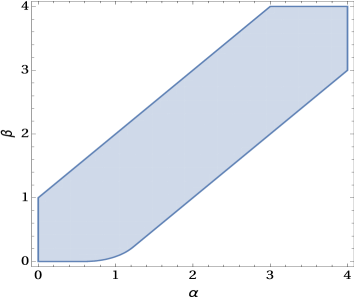
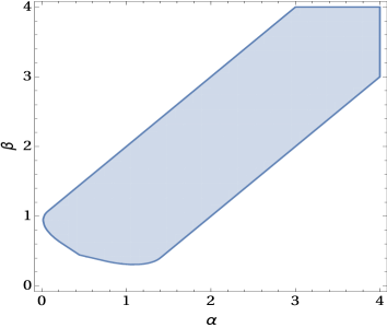
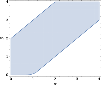
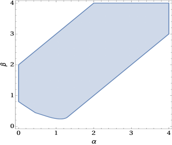
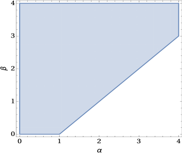
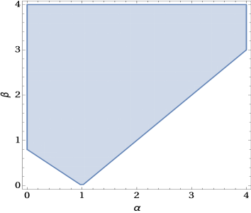
Figure 1. Set $R_{0}(d)$ of all $(\alpha,\beta)$ for which the zeroth-order entropy is dissipating. Left column: $d=2$, right column: $d=10$. Top row: explicit Euler scheme with $C_{\rm RK}=2$, middle row: implicit Euler scheme with $C_{\rm RK}=1$, bottom row: Runge-Kutta scheme of order $p\geq 2$ with $C_{\rm RK}=0$.

Proof.

Since $k\in{\mathbb{N}}$ is fixed, we set $u:=u^{k}$. We choose the functions

$$\Gamma_{1}(u)=c_{1}\beta^{2}u^{2\beta-\alpha-1},\quad\Gamma_{2}(u)=c_{2}\beta^{2}u^{2\beta-2\alpha-1}.$$

It holds $h^{\prime\prime}(u)=u^{\alpha-1}$ and $\mu(u)=\beta u^{\beta-\alpha}$. Then the coefficients in (22) are as follows:

$$a_{1} =\beta^{2}\big{(}(C_{\rm RK}+1)+(1-\tfrac{1}{d})c_{1}\big{)}u^{2\beta-\alpha-1},$$

$$a_{2} =\beta^{2}\big{(}(C_{\rm RK}+2)(\beta-\alpha)+(1-\tfrac{1}{d})(2\beta-\alpha-1)c_{1}-(\tfrac{2}{d}+1)c_{2}\big{)}u^{2\beta-2\alpha-1},$$

$$a_{3} =\beta^{2}\big{(}(\beta-\alpha)^{2}-(2\beta-2\alpha-1)c_{2}\big{)}u^{2\beta-3\alpha-2},$$

$$a_{4} =-\beta^{2}(d-1)\big{(}(2\beta-\alpha-1)c_{1}+2c_{2}\big{)}u^{2\beta-2\alpha-1},$$

$$a_{5} =-\beta^{2}c_{1}u^{2\beta-\alpha-1},\quad a_{6}=-\beta^{2}d(d-1)c_{1}u^{2\beta-\alpha-1}.$$

Introducing the variables $\eta_{j}=\xi_{j}/u^{\alpha}$ for $j\in\{G,L,R,S\}$, we can write (21) as

$$G^{\prime\prime}(0)\leq G^{\prime\prime}(0)+J_{1}+J_{2}=-\beta^{2}\int_{\Omega}u^{2\beta+\alpha-1}Q(\eta)dx,$$

$$\mbox{where }Q(\eta)=b_{1}\eta_{L}^{2}+b_{2}\eta_{L}\eta_{G}^{2}+b_{3}\eta_{G}^{4}+b_{4}\eta_{S}\eta_{G}^{2}+b_{5}\eta_{R}^{2}+b_{6}\eta_{S}^{2}$$

with coefficients

$$b_{1} =(C_{\rm RK}+1)+(1-\tfrac{1}{d})c_{1},$$

$$b_{2} =(C_{\rm RK}+2)(\beta-\alpha)+(1-\tfrac{1}{d})(2\beta-\alpha-1)c_{1}-(\tfrac{2}{d}+1)c_{2},$$

$$b_{3} =(\beta-\alpha)^{2}-(2\beta-2\alpha-1)c_{2},$$

$$b_{4} =-(d-1)\big{(}(2\beta-\alpha-1)c_{1}+2c_{2}\big{)},$$

$$b_{5} =-c_{1},\quad b_{6}=-d(d-1)c_{1}.$$

We need to determine all $(\alpha,\beta)$ such that there exist $c_{1}\leq 0$, $c_{2}\in{\mathbb{R}}$ such that $Q(\eta)\geq 0$ for all $\eta=(\eta_{G},\eta_{L},\eta_{R},\eta_{S})$. Without loss of generality, we exclude the cases $b_{1}=b_{2}=0$ and $b_{4}=b_{6}=0$ since they lead to parameters $(\alpha,\beta)$ included in the region calculated below. Thus, let $b_{1}>0$ and $b_{6}>0$. These inequalities give the bound $-(C_{\rm RK}+1)/(1-1/d)<c_{1}<0$. Thus, we may introduce the parameter $\lambda\in(0,1)$ by setting $c_{1}=-\lambda(C_{\rm RK}+1)/(1-1/d)$. The polynomial $Q(\eta)$ can be rewritten as

$$Q(\eta) =b_{1}\left(\eta_{L}+\frac{b_{2}}{2b_{1}}\eta_{G}^{2}\right)^{2}+b_{6}\left(\eta_{S}+\frac{b_{4}}{2b_{6}}\eta_{G}^{2}\right)^{2}+b_{5}\eta_{R}^{2}+\eta_{G}^{4}\left(b_{3}-\frac{b_{2}^{2}}{4b_{1}}-\frac{b_{4}^{2}}{4b_{6}}\right)$$

$$\geq\eta_{G}^{4}\left(b_{3}-\frac{b_{4}^{2}}{4b_{6}}-\frac{b_{2}^{2}}{4b_{1}}\right)=:\frac{\eta_{G}^{4}(C_{\rm RK}+1)}{4b_{1}b_{6}}R(c_{2};\lambda,\alpha,\beta),$$

where $R(c_{2};\lambda,\alpha,\beta)$ is a quadratic polynomial in $c_{2}$ with the nonpositive leading term $-d^{2}(4-3\lambda)+4(2-3\lambda)d-4$. The polynomial $R(c_{2};\lambda,\alpha,\beta)$ is nonnegative for some $c_{2}$ if and only if its discriminant $4d^{2}\lambda(1-\lambda)S(\lambda;\alpha,\beta)$ is nonnegative. Here, $S(\lambda;\alpha,\beta)$ is a quadratic polynomial in $\lambda$. In order to derive the conditions on $(\alpha,\beta)$ such that $S(\lambda;\alpha,\beta)\geq 0$ for some $\lambda\in(0,1)$, we employ the computer-algebra system Mathematica. The result of the command

Resolve[Exists[LAMBDA, S[LAMBDA] >= 0 && LAMBDA > 0
&& LAMBDA < 1], Reals]Ψ

gives all $(\alpha,\beta)\in{\mathbb{R}}^{2}$ such that there exist $c_{1}\leq 0$, $c_{2}\in{\mathbb{R}}$ such that $Q(\eta)\geq 0$. The interior of this region equals the set $R_{0}(d)$, defined in the statement of the theorem. This shows that $G^{\prime\prime}(0)\leq 0$ for all $(\alpha,\beta)\in R_{0}(d)$.

If $G^{\prime\prime}(0)=0$, the nonnegative polynomial $Q$ has to vanish. In particular, $b_{1}\eta_{L}^{2}=0$. If $\eta_{L}=0$ in $\Omega$, the boundary conditions imply that $u$ is constant, which contradicts our assumption that $u$ is not the steady state. Thus $b_{1}=0$. Similarly, $b_{2}=b_{3}=b_{4}=0$. This gives a system of four inhomogeneous linear equations for $(c_{1},c_{2})$ which is unsolvable. Consequently, $G^{\prime\prime}(0)<0$.

The set $R_{0}(d)$ is nonempty since, e.g., $(1,1)\in R_{0}(d)$. Indeed, choosing $c_{1}=-1$ and $c_{2}=0$, we find that $Q(\eta)=(C_{\rm RK}+\frac{1}{d})\eta_{L}^{2}+\eta_{R}^{2}+d(d-1)\eta_{S}^{2}\geq 0$.

In one space dimension, the situation simplifies since the Laplacian coincides with the Hessian and thus, the integration-by-parts formula (19) is not needed. Then (see (20))

$$G^{\prime\prime}(0)=G^{\prime\prime}(0)+J_{1}=-\beta^{2}\int_{\Omega}u^{2\beta+\alpha-1}\big{(}a_{1}\xi_{L}^{2}+a_{2}\xi_{L}\xi_{G}^{2}+a_{3}\xi_{G}^{4}\big{)}dx,$$

where

$$a_{1}=C_{\rm RK}+1,\quad a_{2}=(C_{\rm RK}+2)(\beta-\alpha)-3c_{2},\quad a_{3}=(\beta-\alpha)^{2}-(2\beta-2\alpha-1)c_{2}.$$

The polynomial $P(\xi)=\xi_{G}^{4}(a_{1}y^{2}+a_{2}y+a_{3})$ with $y=\xi_{L}/\xi_{G}^{2}$ is nonnegative if and only if $a_{1}\geq 0$ and $4a_{1}a_{3}-a_{2}^{2}\geq 0$, which is equivalent to

(24) $$-9c_{2}^{2}+2\big{(}(C_{\rm RK}-2)(\alpha-\beta)+2(C_{\rm RK}+1)\big{)}c_{2}-C_{\rm RK}^{2}(\alpha-\beta)^{2}\geq 0.$$

This inequality has a solution $c_{2}\in{\mathbb{R}}$ if and only if the quadratic polynomial has real roots, i.e. if its discriminant is nonnegative,

$$0 \leq\big{(}(C_{\rm RK}-2)(\alpha-\beta)+2(C_{\rm RK}+1)\big{)}^{2}-9C_{\rm RK}^{2}(\alpha-\beta)^{2}$$

$$=4(C_{\rm RK}+1)\left(-(2C_{\rm RK}-1)(\alpha-\beta)^{2}+(C_{\rm RK}-2)(\alpha-\beta)+(C_{\rm RK}+1)\right).$$

The polynomial $-(2C_{\rm RK}-1)z^{2}+(C_{\rm RK}-2)z+(C_{\rm RK}+1)$ with $z=\alpha-\beta$ is always nonnegative if $C_{\rm RK}=0$ (implicit Euler). For $C_{\rm RK}=1$ and $C_{\rm RK}=2$, this property holds if and only if $-(C_{\rm RK}+1)/(2C_{\rm RK}-1)\leq\alpha-\beta\leq 1$. This concludes the proof. ∎

4.2. First-order entropies

We consider the one-dimensional case and first-order entropies with $f(u)=u^{\alpha/2}$, $\alpha>0$.

Theorem 9.

Let $\Omega\subset{\mathbb{R}}$ be a bounded interval. Let $(u^{k})$ be a sequence of (smooth) solutions to the Runge-Kutta scheme (2) of order $p\geq 2$ for (23) in one space dimension. Let the entropy be given by $F[u]=\int_{\Omega}(u^{\alpha/2})_{x}^{2}dx$ with $\alpha>0$, let $k\in{\mathbb{N}}$ be fixed, and let $u^{k}$ be not the constant steady state of (23). There exists a nonempty region $R_{1}\in[0,\infty)^{2}$ and $\tau^{k}>0$ such that for all $(\alpha,\beta)\in R_{1}$, there is a constant $C_{\alpha,\beta}>0$ such that for all $0<\tau\leq\tau^{k}$,

$$F[u^{k}]+\tau C_{\alpha,\beta}\int_{\Omega}(u^{k})^{\alpha+\beta-3}(u^{k}_{xx})^{2}dx\leq F[u^{k-1}],\quad k\in{\mathbb{N}}.$$

Figure 2 illustrates the set $R_{1}$. The set of admissible values $(\alpha,\beta)$ for the continuous equation is given by $\{-2\leq\alpha-2\beta<1\}$ (the borders of this set are depicted in the figure by the dashed lines).

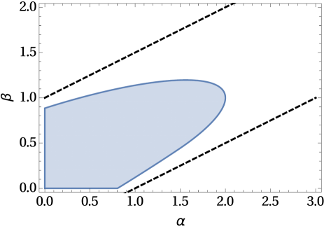
Figure 2. Set of all $(\alpha,\beta)$ for which the discrete first-order entropy for solutions to the one-dimensional porous-medium equation is dissipating. The continuous first-order entropy is dissipated for $-2\leq\alpha-2\beta<1$. The borders of this set is indicated in the figure by dashed lines.

Proof.

First, we compute $G^{\prime}(0)$ according to Theorem 3:

$$G^{\prime}(0)=-\alpha\int_{\Omega}u^{\alpha/2-1}(u^{\alpha/2})_{xx}(u^{\beta})_{xx}dx.$$

We show that $G^{\prime}(0)$ is nonpositive in a certain range of values $(\alpha,\beta)$. We formulate $G^{\prime}(0)$ as

$$G^{\prime}(0)=-\frac{\alpha^{2}\beta}{4}\int_{\Omega}u^{\alpha+\beta-1}\big{(}(\alpha-2)(\beta-1)\xi_{1}^{4}+(\alpha+2\beta-4)\xi_{1}^{2}\xi_{2}+2\xi_{2}^{2}\big{)}dx,$$

where $\xi_{1}=u_{x}/u$, $\xi_{2}=u_{xx}/u$. We employ the integration-by-parts formula

$$0=\int_{\Omega}(u^{\alpha+\beta-4}u_{x}^{3})_{x}dx=\int_{\Omega}u^{\alpha+\beta-1}\big{(}(\alpha+\beta-4)\xi_{1}^{4}+3\xi_{1}^{2}\xi_{2}\big{)}dx=:J.$$

Therefore,

$$G^{\prime}(0)=G^{\prime}(0)-\frac{\alpha^{2}\beta}{4}cJ=-\frac{\alpha^{2}\beta}{4}\int_{\Omega}u^{\alpha+\beta-1}P(\xi)dx,$$

where

$$P(\xi)=\big{(}(\alpha-2)(\beta-1)+(\alpha+\beta-4)c\big{)}\xi_{1}^{4}+\big{(}\alpha+2\beta-4+3c\big{)}\xi_{1}^{2}\xi_{2}+2\xi_{2}^{2}.$$

This polynomial is nonnegative if and only if

$$8\big{(}(\alpha-2)(\beta-1)+(\alpha+\beta-4)c\big{)}-(\alpha+2\beta-4+3c)^{2}\geq 0,$$

which is equivalent to

$$g(c):=-9c^{2}+2(\alpha-2\beta-4)c-(\alpha-2\beta)^{2}\geq 0.$$

The maximizing value $c^{*}=(\alpha-2\beta-4)/9$, obtained from $g^{\prime}(c)=0$, yields

$$g(c^{*})=-\frac{8}{9}(\alpha-2\beta-1)(\alpha-2\beta+2)\geq 0$$

and consequently $G^{\prime}(0)\leq 0$ if $-2\leq\alpha-2\beta\leq 1$. This condition is the same as in [6, Theorem 13] for the continuous equation.

Next, we turn to the proof of $G^{\prime\prime}(0)<0$. The proof of Theorem 3 shows that

$$G^{\prime\prime}(0) =-\frac{\alpha}{2}\int_{\Omega}\bigg{(}\frac{\alpha}{2}\big{(}u^{\alpha/2-1}(u^{\beta})_{xx}\big{)}_{x}^{2}-\bigg{(}\frac{\alpha}{2}-1\bigg{)}u^{\alpha/2-2}(u^{\alpha/2})_{xx}(u^{\beta})_{xx}^{2}$$

$$\phantom{xx}{}-\beta C_{\rm RK}u^{\alpha/2-1}(u^{\alpha/2})_{xx}\big{(}u^{\beta-1}(u^{\beta})_{xx}\big{)}_{xx}\bigg{)}dx.$$

We integrate by parts in the last term and use $(\beta u^{\beta-1}(u^{\beta})_{xx})_{x}=0$ on $\partial\Omega$:

$$G^{\prime\prime}(0) =-\frac{1}{8}\alpha^{2}\beta^{2}\int_{\Omega}u^{\alpha+2\beta-2}$$

$$\phantom{xx}{}\times\big{(}a_{1}\xi_{1}^{6}+a_{2}\xi_{1}^{4}\xi_{2}+a_{3}\xi_{1}^{3}\xi_{3}+a_{4}\xi_{1}^{2}\xi_{2}^{2}+a_{5}\xi_{1}\xi_{2}\xi_{3}+a_{6}\xi_{2}^{3}+a_{7}\xi_{3}^{2}\big{)}dx,$$

where $\xi_{1}=u_{x}/u$, $\xi_{2}=u_{xx}/u$, $\xi_{3}=u_{xxx}/u$, and

$$a_{1} =(\beta-1)\big{(}2C_{\rm RK}\alpha^{2}\beta-3C_{\rm RK}\alpha^{2}+2\alpha\beta^{2}-2(5C_{\rm RK}+3)\alpha\beta+(15C_{\rm RK}+4)\alpha$$

$$\phantom{xx}{}+2\beta^{3}-14\beta^{2}+4(3C_{\rm RK}+7)\beta-2(9C_{\rm RK}+8)\big{)},$$

$$a_{2} =(\beta-1)\big{(}4C_{\rm RK}\alpha^{2}+(8C_{\rm RK}+7)\alpha\beta-(32C_{\rm RK}+9)\alpha+12\beta^{2}-2(8C_{\rm RK}+25)\beta$$

$$\phantom{xx}{}+6(8C_{\rm RK}+7)\big{)},$$

$$a_{3} =C_{\rm RK}\alpha^{2}+2\alpha\beta-(5C_{\rm RK}+2)\alpha+4(C_{\rm RK}+1)\beta^{2}-2(5C_{\rm RK}+8)\beta+12(C_{\rm RK}+1),$$

$$a_{4} =2(\beta-1)\big{(}2(4C_{\rm RK}+1)\alpha+9\beta-(16C_{\rm RK}+13)\big{)},$$

$$a_{5} =2(2C_{\rm RK}+1)\alpha+4(2C_{\rm RK}+3)\beta-16(C_{\rm RK}+1),$$

$$a_{6} =2-\alpha,\quad a_{7}=2(C_{\rm RK}+1).$$

We employ three integration-by-parts formulas:

$$0 =\int_{\Omega}\big{(}u^{\alpha+2\beta-5}u_{xx}^{2}u_{x}\big{)}_{x}dx=\int_{\Omega}u^{\alpha+2\beta-2}\big{(}(\alpha+2\beta-5)\xi_{1}^{2}\xi_{2}^{2}+2\xi_{1}\xi_{2}\xi_{3}+\xi_{2}^{3}\big{)}dx=:J_{1},$$

$$0 =\int_{\Omega}\big{(}u^{\alpha+2\beta-6}u_{xx}u_{x}^{3}\big{)}_{x}dx=\int_{\Omega}u^{\alpha+2\beta-2}\big{(}(\alpha+2\beta-6)\xi_{1}^{4}\xi_{2}+\xi_{1}^{3}\xi_{3}+3\xi_{1}^{2}\xi_{2}^{2}\big{)}dx=:J_{2},$$

$$0 =\int_{\Omega}\big{(}u^{\alpha+2\beta-7}u_{x}^{5}\big{)}_{x}dx=\int_{\Omega}u^{\alpha+2\beta-2}\big{(}(\alpha+2\beta-7)\xi_{1}^{6}+5\xi_{1}^{4}\xi_{2}\big{)}dx=:J_{3}.$$

Then

$$G^{\prime\prime}(0)=G^{\prime\prime}(0)-\frac{1}{8}\alpha^{2}\beta^{2}(c_{1}J_{1}+c_{2}J_{2}+c_{3}J_{3})=-\frac{1}{8}\alpha^{2}\beta^{2}\int_{\Omega}u^{\alpha+2\beta-2}P(\xi)dx,$$

$$\mbox{where }P(\xi)=b_{1}\xi_{1}^{6}+b_{2}\xi_{1}^{4}\xi_{2}+b_{3}\xi_{1}^{3}\xi_{3}+b_{4}\xi_{1}^{2}\xi_{2}^{2}+b_{5}\xi_{1}\xi_{2}\xi_{3}+b_{6}\xi_{2}^{3}+b_{7}\xi_{3}^{2},$$

and the coefficients are given by

$$b_{1} =a_{1}+(\alpha+2\beta-7)c_{3}, b_{2} =a_{2}+(\alpha+2\beta-6)c_{2}+5c_{3},$$

$$b_{3} =a_{3}+c_{2}, b_{4} =a_{4}+(\alpha+2\beta-5)c_{1}+3c_{2},$$

$$b_{5} =a_{5}+2c_{1}, b_{6} =a_{6}+c_{1},$$

$$b_{7} =a_{7}.$$

Choosing $c_{1}=-a_{6}$, we eliminate the cubic term $\xi_{2}^{3}$. Furthermore, setting, $x=\xi_{2}/\xi_{1}^{2}$ and $y=\xi_{3}/\xi_{1}^{3}$, we can write the polynomial $P$ as a quadratic polynomial in $(x,y)$:

$$Q(x,y)=\xi_{1}^{6}P(\xi)=b_{1}+b_{2}x+b_{3}y+b_{4}x^{2}+b_{5}xy+b_{7}y^{2}.$$

The following lemma is a consequence of the proof of Lemma 2.2 in [16].

Lemma 10.

The polynomial $p(x,y)=A+Bx+Cy+Dx^{2}+Exy+Fy^{2}$ with $F>0$ is nonnegative for all $(x,y)\in{\mathbb{R}}^{2}$ if and only if

$$\text{\rm(i)}\phantom{.}\quad 4DF-E^{2}>0\quad\mbox{and}\quad A(4DF-E^{2})-B^{2}F-C^{2}D+BCE\geq 0,\quad\mbox{or}$$

$$\text{\rm(ii)}\quad 4DF-E^{2}=0\quad\mbox{and}\quad 2BF-CE=0\quad\mbox{and}\quad 4AF-C^{2}\geq 0.$$

Note that in case $4DF-E^{2}=0$ and $E\neq 0$, we may replace $2BF-CE=0$ by the condition $2BEF=CE^{2}=4CDF$ or (since $F>0$) $BE=2CD$.

The first inequality in case (i),

$$0 <4b_{4}b_{7}-b_{5}^{2}=-(C_{\rm RK}+1)(2C_{\rm RK}+1)\alpha^{2}+(2C_{\rm RK}+2)(4C_{\rm RK}-3)\alpha\beta+(9C_{\rm RK}+9)\alpha$$

$$\phantom{xx}{}-2C_{\rm RK}(4C_{\rm RK}+3)\beta^{2}+(8C_{\rm RK}+12)\beta+(3C_{\rm RK}+3)c_{2}-(12C_{\rm RK}+14),$$

is linear in $c_{2}$ and provides a lower bound for $c_{2}$:

$$c_{2} >\frac{1}{3(C_{\rm RK}+1)}\Big{(}(C_{\rm RK}+1)(2C_{\rm RK}+1)\alpha^{2}-(2C_{\rm RK}+2)(4C_{\rm RK}-3)\alpha\beta-(9C_{\rm RK}+9)\alpha$$

$$\phantom{xx}{}+2C_{\rm RK}(4C_{\rm RK}+3)\beta^{2}-(8C_{\rm RK}+12)\beta+(12C_{\rm RK}+14)\Big{)}=:c_{2}^{*}.$$

The second inequality in case (i) becomes

$$0\leq b_{1}(4b_{4}b_{7}-b_{5}^{2})-b_{2}^{2}b_{7}-b_{3}^{2}b_{4}+b_{2}b_{3}b_{5}=-50(C_{\rm RK}+1)c_{3}^{2}+p_{1}(\alpha,\beta,c_{2})c_{3}+p_{2}(\alpha,\beta,c_{2}),$$

where $p_{1}$ and $p_{2}$ are some polynomials in $\alpha$, $\beta$, and $c_{2}$. This quadratic expression in $c_{3}$ is nonnegative if and only if its discriminant is nonnegative,

$$0 \leq-200(C_{\rm RK}+1)p_{2}(\alpha,\beta,c_{2})-p_{1}(\alpha,\beta,c_{2})^{2}$$

$$=-8\big{(}4b_{4}b_{7}-b_{5}^{2}\big{)}\big{(}25c_{2}^{2}+p_{3}(\alpha,\beta)c_{2}+p_{4}(\alpha,\beta)\big{)},$$

where $p_{3}(\alpha,\beta)$ and $p_{4}(\alpha,\beta)$ are some polynomials in $\alpha$ and $\beta$. The factor $4b_{4}b_{7}-b_{5}^{2}$ is positive, so we have to ensure that $R_{\alpha,\beta}(c_{2})=25c_{2}^{2}+p_{3}(\alpha,\beta)c_{2}+p_{4}(\alpha,\beta)\leq 0$ for some $c_{2}>c_{2}^{*}$. Therefore we must ensure that the rightmost root of $R_{\alpha,\beta}(c_{2})$ is larger or equal than the lower bound for $c_{2}$, i.e., $-p_{3}(\alpha,\beta)+\sqrt{p_{3}^{2}(\alpha,\beta)-100p_{4}(\alpha,\beta)}\geq 50c^{*}_{2}$. For $C_{\rm RK}=1$, the values $(\alpha,\beta)$ for which there exists $c_{2}>c_{2}^{*}$ such that $R_{\alpha,\beta}(c_{2})\leq 0$ is depicted in Figure 2. In case (ii), we may immediately calculate $c_{2}$ and $c_{3}$ but this results in a region which is already contained in the first one. This shows that $G^{\prime\prime}(0)\leq 0$.

If $G^{\prime\prime}(0)=0$, the polynomial $Q$ vanishes. Thus, either $u_{x}/u=\xi_{1}=0$ or $P(\xi)=0$ in $\Omega$. The first case is impossible since $u$ is not constant in $\Omega$. As $b_{7}=a_{7}=2(C_{\rm RK}+1)>0$, the second case $P(\xi)=0$ implies that $\xi_{3}=0$. Hence, $u$ is a quadratic polynomial. In view of the boundary conditions, $u$ must be constant, but this contradicts our assumption. Hence, $G^{\prime\prime}(0)<0$. ∎

5. Linear diffusion system

We consider the following linear diffusion system:

(25) $$\partial_{t}u_{1}-\rho_{1}\Delta u_{1}=\mu(u_{2}-u_{1}),\quad\partial_{t}u_{2}-\rho_{2}\Delta u_{2}=\mu(u_{1}-u_{2}),$$

with initial and homogeneous Neumann boundary conditions, $\rho_{1}$, $\rho_{2}$, $\mu>0$, and the entropy

(26) $$H[u]=\int_{\Omega}h(u)dx=\int_{\Omega}\sum_{i=1}^{2}u_{i}(\log u_{i}-1)dx,$$

where $u=(u_{1},u_{2})$. If the initial data is nonnegative, the maximum principle shows that the solutions to (25) are nonnegative too.

Theorem 11.

Let $(u^{k})$ be a sequence of (smooth) nonnegative solutions to the Runge-Kutta scheme (2) for (25) with $C_{\rm RK}=1$ and $\rho:=\rho_{1}=\rho_{2}$. Let the entropy $H$ be given by (26). Let $k\in{\mathbb{N}}$ be fixed and let $u^{k}$ be not the steady state of (2). Then there exists $\tau^{k}>0$ such that for all $0<\tau<\tau^{k}$,

$$H[u^{k}]+\tau\int_{\Omega}\bigg{(}\rho\sum_{i=1}^{2}\frac{|\nabla u_{i}^{k}|^{2}}{u_{i}^{k}}+\mu(\log u_{1}^{k}-\log u_{2}^{k})(u_{1}^{k}-u_{2}^{k})\bigg{)}dx\leq H[u^{k-1}].$$

Note that we need equal diffusivities $\rho_{1}=\rho_{2}$ and higher-order schemes ($C_{\rm RK}=1$). These conditions are in accordance of [18], where the continuous equation was studied. In order to highlight the step where these conditions are needed, the following proof is slightly more general than actually needed.

Proof.

We fix $k\in{\mathbb{N}}$ and set $u:=u^{k}$. Let $A[u]=(A_{1}[u],A_{2}[u])=(\rho_{1}\Delta u_{1}+\mu(u_{2}-u_{1}),\rho_{2}\Delta u_{2}+\mu(u_{1}-u_{2}))$. Since $A$ is linear, $DA[u](h)=A[h]$. Thus,

$$G^{\prime\prime}(0)=-\int_{\Omega}\big{(}C_{\rm RK}h^{\prime}(u)^{\top}A[A[u]]+A[u]^{\top}h^{\prime\prime}(u)A[u]\big{)}dx=-G_{1}-G_{2}.$$

In the following, we set $\partial_{i}h=\partial h/\partial u_{i}$ for $i=1,2$. We integrate by parts twice, using the boundary conditions $\nabla u_{i}\cdot\nu=0$ and $\nabla A_{i}[u]\cdot\nu=0$ on $\partial\Omega$, and collect the terms:

$$G_{1} =C_{\rm RK}\int_{\Omega}\Big{(}\partial_{1}h(u)\big{(}\rho_{1}\Delta A_{1}[u]+\mu(A_{2}[u]-A_{1}[u])\big{)}$$

$$\phantom{xx}{}+\partial_{2}h(u)\big{(}\rho_{2}\Delta A_{2}[u]+\mu(A_{1}[u]-A_{2}[u])\big{)}\Big{)}dx$$

$$=C_{\rm RK}\int_{\Omega}\Big{(}\rho_{1}\Delta\partial_{1}h(u)A_{1}[u]+\rho_{2}\Delta\partial_{2}h(u)A_{2}[u]$$

$$\phantom{xx}{}+\mu(\partial_{1}h(u)-\partial_{2}h(u))(A_{2}[u]-A_{1}[u])\Big{)}dx$$

$$=C_{\rm RK}\int_{\Omega}\Big{(}\rho_{1}\big{(}\partial_{1}^{2}h(u)\Delta u_{1}+\partial_{1}^{3}h(u)|\nabla u_{1}|^{2}\big{)}\big{(}\rho_{1}\Delta u_{1}+\mu(u_{2}-u_{1})\big{)}$$

$$\phantom{xx}{}+\rho_{2}\big{(}\partial_{2}^{2}h(u)\Delta u_{2}+\partial_{2}^{3}h(u)|\nabla u_{2}|^{2}\big{)}\big{(}\rho_{2}\Delta u_{2}+\mu(u_{1}-u_{2})\big{)}$$

$$\phantom{xx}{}+\mu(\partial_{2}h(u)-\partial_{1}h(u))\big{(}\rho_{1}\Delta u_{1}-\rho_{2}\Delta u_{2}+2\mu(u_{2}-u_{1})\big{)}\Big{)}dx$$

$$=C_{\rm RK}\int_{\Omega}\Big{(}\rho_{1}^{2}\partial_{1}^{2}h(u)(\Delta u_{1})^{2}+\rho_{2}^{2}\partial_{2}^{2}h(u)(\Delta u_{2})^{2}+\rho_{1}^{2}\partial_{1}^{3}h(u)\Delta u_{1}|\nabla u_{1}|^{2}$$

$$\phantom{xx}{}+\rho_{2}^{2}\partial_{2}^{3}h(u)\Delta u_{2}|\nabla u_{2}|^{2}+\rho_{1}\mu\big{(}\partial_{1}^{2}h(u)(u_{2}-u_{1})+\partial_{2}h(u)-\partial_{1}h(u)\big{)}\Delta u_{1}$$

$$\phantom{xx}{}+\rho_{2}\mu\big{(}\partial_{2}^{2}h(u)(u_{1}-u_{2})+\partial_{1}h(u)-\partial_{2}h(u)\big{)}\Delta u_{2}+\rho_{1}\mu\partial_{1}^{3}h(u)(u_{2}-u_{1})|\nabla u_{1}|^{2}$$

$$\phantom{xx}{}+\rho_{2}\mu\partial_{2}^{3}h(u)(u_{1}-u_{2})|\nabla u_{2}|^{2}+2\mu^{2}(\partial_{2}h(u)-\partial_{1}h(u))(u_{2}-u_{1})\Big{)}dx.$$

Furthermore,

$$G_{2} =\int_{\Omega}\Big{(}\partial_{1}^{2}h(u)\big{(}\rho_{1}\Delta u_{1}+\mu(u_{2}-u_{1})\big{)}^{2}+\partial_{2}^{2}h(u)\big{(}\rho_{2}\Delta u_{2}+\mu(u_{1}-u_{2})\big{)}^{2}\Big{)}dx$$

$$=\int_{\Omega}\Big{(}\rho_{1}^{2}\partial_{1}^{2}h(u)(\Delta u_{1})^{2}+\rho_{2}^{2}\partial_{2}^{2}h(u)(\Delta u_{2})^{2}+2\rho_{1}\mu\partial_{1}^{2}h(u)(u_{2}-u_{1})\Delta u_{1}$$

$$\phantom{xx}{}+2\rho_{2}\mu\partial_{2}^{2}h(u)(u_{1}-u_{2})\Delta u_{2}+\mu^{2}(\partial_{1}^{2}h(u)+\partial_{2}^{2}h(u))(u_{1}-u_{2})^{2}\Big{)}dx.$$

Adding $G_{1}$ and $G_{2}$, we arrive at

$$G^{\prime\prime}(0) =-\sum_{i=1}^{2}\int_{\Omega}\Big{(}\rho_{i}^{2}(C_{\rm RK}+1)\partial_{i}^{2}h(u)(\Delta u_{i})^{2}+\rho_{i}^{2}C_{\rm RK}\partial_{i}^{3}h(u)\Delta u_{i}|\nabla u_{i}|^{2}\Big{)}dx$$

$$\phantom{xx}{}-\int_{\Omega}\Big{(}\rho_{1}\mu\big{(}(C_{\rm RK}+2)\partial_{1}^{2}h(u)(u_{2}-u_{1})+C_{\rm RK}(\partial_{2}h(u)-\partial_{1}h(u))\big{)}\Delta u_{1}$$

$$\phantom{xx}{}+\rho_{2}\mu\big{(}(C_{\rm RK}+2)\partial_{2}^{2}h(u)(u_{1}-u_{2})+C_{\rm RK}(\partial_{1}h(u)-\partial_{2}h(u))\big{)}\Delta u_{2}$$

$$\phantom{xx}{}+\rho_{1}\mu C_{\rm RK}\partial_{1}^{3}h(u)(u_{2}-u_{1})|\nabla u_{1}|^{2}+\rho_{2}\mu C_{\rm RK}\partial_{2}^{3}h(u)(u_{1}-u_{2})|\nabla u_{2}|^{2}\Big{)}dx$$

$$\phantom{xx}{}-\int_{\Omega}\mu^{2}\Big{(}2(\partial_{1}h(u)-\partial_{2}h(u))+(\partial_{1}^{2}h(u)+\partial_{2}^{2}h(u))(u_{1}-u_{2})\Big{)}(u_{1}-u_{2})dx$$

$$=-I_{2}-I_{1}-I_{0}.$$

The idea of [18] is to show that each integral $I_{i}$, involving only derivatives of order $i$, is nonnegative. In contrast to [18], we employ systematic integration by parts, which allows for a simpler and more general proof in our context. For the term $I_{2}$, we use the following integration-by-parts formula:

$$0=\int_{\Omega}\operatorname{div}\big{(}u_{i}^{-2}|\nabla u_{i}|^{3}\big{)}dx=\int_{\Omega}\big{(}-2u_{i}^{-3}|\nabla u_{i}|^{4}+3u_{i}^{-2}\Delta u_{i}|\nabla u_{i}|^{2}\big{)}dx=:J_{i}.$$

Then, for $\varepsilon>0$,

$$I_{2}-c\sum_{i=1}^{2}\rho_{i}^{2}J_{i}-\varepsilon\sum_{i=1}^{2}u_{i}^{-3}|\nabla u_{i}|^{4}dx$$

$$=\sum_{i=1}^{2}\rho^{2}_{i}\int_{\Omega}\Big{(}(C_{\rm RK}+1)u_{i}^{-1}(\Delta u_{i})^{2}-(3c+C_{\rm RK})u_{i}^{-2}\Delta u_{i}|\nabla u_{i}|^{2}+(2c-\varepsilon)u_{i}^{-3}|\nabla u_{i}|^{4}\Big{)}dx.$$

The integrand defines a quadratic polynomial in the variables $\Delta u_{i}$ and $|\nabla u_{i}|^{2}$ and is nonnegative if its discriminant satisfies $4(2c-\varepsilon)(C_{\rm RK}+1)-(3c+C_{\rm RK})^{2}\geq 0$. It turns out that this inequality holds true for $C_{\rm RK}\in\{0,1\}$ if we choose $c=2/3$ and $\varepsilon>0$ sufficiently small. When $C_{\rm RK}=2$, we can show only that $I_{2}\geq 0$ which is not sufficient to prove that $G^{\prime\prime}(0)<0$ (see below). We conclude that

(27) $$I_{2}\geq\varepsilon\sum_{i=1}^{2}\int_{\Omega}u_{i}^{-3}|\nabla u_{i}|^{4}dx.$$

Integrating by parts in $I_{1}$ in order to obtain only first-order derivatives, we find after some rearrangements that

$$I_{1} =\mu\int_{\Omega}\big{(}a_{1}|\nabla\log u_{1}|^{2}+a_{2}\nabla\log u_{1}\cdot\nabla\log u_{2}+a_{3}|\nabla\log u_{2}|^{2}\big{)}dx,\quad\mbox{where}$$

$$a_{1} =2\rho_{1}(C_{\rm RK}u_{1}+u_{2}),\quad a_{3}=2\rho_{2}(C_{\rm RK}u_{2}+u_{1}),$$

$$a_{2} =-(C_{\rm RK}(\rho_{1}+\rho_{2})+2\rho_{2})u_{1}-(C_{\rm RK}(\rho_{1}+\rho_{2})+2\rho_{1})u_{2}.$$

The integrand is nonnegative if and only if $4a_{1}a_{3}-a_{2}^{2}\geq 0$ for all $(u_{1},u_{2})$. We compute:

$$C_{\rm RK}=0: \quad 4a_{1}a_{3}-a_{2}^{2}=-4(\rho_{1}u_{2}-\rho_{2}u_{1})^{2},$$

$$C_{\rm RK}=1: \quad 4a_{1}a_{3}-a_{2}^{2}=(\rho_{1}-\rho_{2})\big{(}\rho_{1}(u_{1}^{2}+6u_{1}u_{2}+9u_{2}^{2})-\rho_{2}(9u_{1}^{2}+6u_{1}u_{2}+u_{2}^{2})\big{)},$$

$$C_{\rm RK}=2: \quad 4a_{1}a_{3}-a_{2}^{2}=-4\big{(}\rho_{1}(u_{1}+2u_{2})-\rho_{2}(2u_{1}+u_{2})\big{)}.$$

Thus, $4a_{1}a_{3}-a_{2}^{2}\geq 0$ is possible only if $\rho_{1}=\rho_{2}$ and $C_{\rm RK}=1$.

Finally, we see immediately that the remaining term

$$I_{0}=\mu^{2}\int_{\Omega}\bigg{(}2(\log u_{1}-\log u_{2})(u_{1}-u_{2})+\bigg{(}\frac{1}{u_{1}}+\frac{1}{u_{2}}\bigg{)}(u_{1}-u_{2})^{2}\bigg{)}dx$$

is nonnegative. This shows that $G^{\prime\prime}(0)\leq 0$. If $G^{\prime\prime}(0)=0$, we infer from (27) that $u_{i}=\mbox{const.}$, but this contradicts our hypothesis that $u_{i}$ is not a steady state. ∎

6. The Derrida-Lebowith-Speer-Spohn equation

Consider the one-dimensional fourth-order equation

(28) $$\partial_{t}u=-(u(\log u)_{xx})_{xx}\quad\mbox{in }\Omega,\ t>o,\quad u(0)=u^{0}$$

with periodic boundary conditions. This equation appears as a scaling limit of the so-called (time-discrete) Toom model, which describes interface fluctuations in a two-dimensional spin system [9]. The variable $u$ is the limit of a random variable related to the deviation of the spin interface from a straight line. The multi-dimensional version of (28) models the eectron density $u$ in a quantum semiconductor, und the equation is the zero-temperature, zero-field approximation of the quantum drift-diffusion model [13]. For existence results for (28), we refer to [15] and references therein.

To simplify our calculations, we analyze only the logarithmic entropy $H[u]=\int_{\Omega}u(\log u-1)dx$. It is possible to verify condition (6) also for entropies of the form $\int_{\Omega}u^{\alpha}dx$, but it turns out that only sufficiently small $\alpha>0$ are admissible (about $0<\alpha<0.15\ldots$) and the computations are very tedious. Therefore, we restrict ourselves to the case $\alpha=0$.

Theorem 12.

Let $(u^{k})$ be a sequence of (smooth) solutions to the Runge-Kutta scheme (2) with $C_{\rm RK}=1$ for (28). Let the entropy be given by $H[u]=\int_{\Omega}u(\log u-1)dx$, let $k\in{\mathbb{N}}$ be fixed, and let $u^{k}$ be not a steady state. Then there exists $\tau^{k}>0$ such that for all $0<\tau<\tau^{k}$,

$$H[u^{k}]+\tau q\int_{\Omega}u(\log u)_{x}^{8}dx+\tau\int_{\Omega}u(\log u)_{xx}^{2}dx\leq H[u^{k-1}],\quad q\approx 0.0045.$$

Proof.

First, we observe that $G^{\prime}(0)=-\int_{\Omega}(u(\log u)_{xx})_{xx}\log udx=-\int_{\Omega}u(\log u)_{xx}^{2}dx$. With $A[u]=(u(\log u)_{xx})_{xx}$ and $DA[u](h)=\big{(}h_{xx}-2(\log u)_{x}h_{x}+(\log u)_{x}^{2}h\big{)}_{xx}$, we can write $G^{\prime\prime}(0)=-I_{0}^{k}$ according to (6) as

$$G^{\prime\prime}(0) =-\int_{\Omega}\Big{(}\log u\big{(}A[u]_{xx}-2(\log u)_{x}A[u]_{x}+(\log u)_{x}^{2}A[u]\big{)}_{xx}+\frac{1}{u}A[u]^{2}\Big{)}dx$$

$$=-\int_{\Omega}\Big{(}(\log u)_{xx}\big{(}A[u]_{xx}-2(\log u)_{x}A[u]_{x}+(\log u)_{x}^{2}A[u]\big{)}+\frac{1}{u}A[u]^{2}\Big{)}dx$$

$$=-\int_{\Omega}\Big{(}\big{(}v_{xxxx}+2(v_{x}v_{xx})_{x}+v_{x}^{2}v_{xx}\big{)}A[u]+\frac{1}{u}A[u]^{2}\Big{)}dx,$$

where we have integrated by parts several times and have set $v=\log u$. Then $A[u]=u(v_{x}^{2}v_{xx}+2v_{x}v_{xxx}+v_{xx}^{2}+v_{xxxx})$ and, with the abbreviations $\xi_{1}=v_{x},\ldots,\xi_{4}=v_{xxxx}$,

$$G^{\prime\prime}(0) =-\int_{\Omega}u\Big{(}2\xi_{1}^{4}\xi_{2}^{2}+8\xi_{1}^{3}\xi_{2}\xi_{3}+5\xi_{1}^{2}\xi_{2}^{3}+4\xi_{1}^{2}\xi_{2}\xi_{4}+8\xi_{1}^{2}\xi_{3}^{2}+10\xi_{1}\xi_{2}^{2}\xi_{3}$$

$$\phantom{xx}{}+8\xi_{1}\xi_{3}\xi_{4}+3\xi_{2}^{4}+5\xi_{2}^{2}\xi_{4}+2\xi_{4}^{2}\Big{)}dx.$$

We employ the following integration-by-parts formulas:

$$0 =\int_{\Omega}(uv_{x}^{7})_{x}dx=\int_{\Omega}u(\xi_{1}^{8}+7\xi_{1}^{6}\xi_{2})dx=:J_{1},$$

$$0 =\int_{\Omega}(uv_{xx}v_{x}^{5})_{x}dx=\int_{\Omega}u(\xi_{1}^{6}\xi_{2}+\xi_{1}^{5}\xi_{3}+5\xi_{1}^{4}\xi_{2}^{2})dx=:J_{2},$$

$$0 =\int_{\Omega}(uv_{xxx}v_{x}^{4})_{x}dx=\int_{\Omega}u(\xi_{1}^{5}\xi_{3}+\xi_{1}^{4}\xi_{4}+4\xi_{1}^{3}\xi_{2}\xi_{3})dx=:J_{3},$$

$$0 =\int_{\Omega}(uv_{xx}^{2}v_{x}^{3})_{x}dx=\int_{\Omega}u(\xi_{1}^{4}\xi_{2}^{2}+2\xi_{1}^{3}\xi_{2}\xi_{3}+3\xi_{1}^{2}\xi_{2}^{3})dx=:J_{4},$$

$$0 =\int_{\Omega}(uv_{xx}v_{xxx}v_{x}^{2})_{x}dx=\int_{\Omega}u(\xi_{1}^{3}\xi_{2}\xi_{3}+\xi_{1}^{2}\xi_{2}\xi_{4}+\xi_{1}^{2}\xi_{3}^{2}+2\xi_{1}\xi_{2}^{2}\xi_{3})dx=:J_{5},$$

$$0 =\int_{\Omega}(uv_{xxx}^{2}v_{x})_{x}dx=\int_{\Omega}u(\xi_{1}^{2}\xi_{3}^{2}+2\xi_{1}\xi_{3}\xi_{4}+\xi_{2}\xi_{3}^{2})dx=:J_{6},$$

$$0 =\int_{\Omega}(uv_{xx}^{3}v_{x})_{x}dx=\int_{\Omega}u(\xi_{1}^{2}\xi_{2}^{3}+3\xi_{1}\xi_{2}^{2}\xi_{3}+\xi_{2}^{4})dx=:J_{7},$$

$$0 =\int_{\Omega}(uv_{xxx}v_{xx}^{2})_{x}dx=\int_{\Omega}u(\xi_{1}\xi_{2}^{2}\xi_{3}+2\xi_{2}\xi_{3}^{2}+\xi_{2}^{2}\xi_{4})dx=:J_{8}.$$

Then

$$G^{\prime\prime}(0) =G^{\prime\prime}(0)-4\sum_{i=1}^{8}c_{i}J_{i}=-\int_{\Omega}u\Big{(}a_{1}\xi_{1}^{8}+a_{2}\xi_{1}^{6}\xi_{2}+a_{3}\xi_{1}^{5}\xi_{3}+a_{4}\xi_{1}^{4}\xi_{2}^{2}+a_{5}\xi_{1}^{4}\xi_{4}$$

$$\phantom{xx}{}+a_{6}\xi_{1}^{3}\xi_{2}\xi_{3}+a_{7}\xi_{1}^{2}\xi_{2}^{3}+a_{8}\xi_{1}^{2}\xi_{2}\xi_{4}+a_{9}\xi_{1}^{2}\xi_{3}^{2}+a_{10}\xi_{1}\xi_{2}^{2}\xi_{3}+a_{11}\xi_{1}\xi_{3}\xi_{4}+a_{12}\xi_{2}^{4}$$

$$\phantom{xx}{}+a_{13}\xi_{2}^{2}\xi_{4}+a_{14}\xi_{2}\xi_{3}^{2}+a_{15}\xi_{4}^{2}\Big{)}dx,$$

where

$$a_{1} =4c_{1}, a_{2} =28c_{1}+4c_{2}, a_{3} =4c_{2}+4c_{3},$$

$$a_{4} =2+20c_{2}+4c_{4}, a_{5} =4c_{3}, a_{6} =8+16c_{3}+8c_{4}+4c_{5},$$

$$a_{7} =5+12c_{4}+4c_{7}, a_{8} =4+4c_{5}, a_{9} =8+4c_{5}+4c_{6},$$

$$a_{10} =10+8c_{5}+12c_{7}+4c_{8}, a_{11} =8+8c_{6}, a_{12} =3+4c_{7},$$

$$a_{13} =5+4c_{8}, a_{14} =4c_{6}+8c_{8}, a_{15} =2.$$

Next, we eliminate all terms involving $\xi_{4}$ by formulating the following square:

$$G^{\prime\prime}(0)=-\int_{\Omega}u\bigg{[}a_{15}\bigg{(}\xi_{4}+\frac{a_{5}}{2a_{15}}\xi_{1}^{4}+\frac{a_{8}}{2a_{15}}\xi_{1}^{2}\xi_{2}+\frac{a_{11}}{2a_{15}}\xi_{1}\xi_{3}+\frac{a_{13}}{2a_{15}}\xi_{2}^{2}\bigg{)}^{2}$$

$$\phantom{xx}{}+\bigg{(}a_{1}-\frac{a_{5}^{2}}{4a_{15}}\bigg{)}\xi_{1}^{8}+\bigg{(}a_{2}-\frac{a_{5}a_{8}}{2a_{15}}\bigg{)}\xi_{1}^{6}\xi_{2}+\bigg{(}a_{3}-\frac{a_{5}a_{11}}{2a_{15}}\bigg{)}\xi_{1}^{5}\xi_{3}$$

$$\phantom{xx}{}+\bigg{(}a_{4}-\frac{a_{8}^{2}}{4a_{15}}-\frac{a_{5}a_{13}}{2a_{15}}\bigg{)}\xi_{1}^{4}\xi_{2}^{2}+\bigg{(}a_{6}-\frac{a_{8}a_{11}}{2a_{15}}\bigg{)}\xi_{1}^{3}\xi_{2}\xi_{3}+\bigg{(}a_{7}-\frac{a_{8}a_{13}}{2a_{15}}\bigg{)}\xi_{1}^{2}\xi_{2}^{3}$$

$$\phantom{xx}{}+\bigg{(}a_{9}-\frac{a_{11}^{2}}{4a_{15}}\bigg{)}\xi_{1}^{2}\xi_{3}^{2}+\bigg{(}a_{10}-\frac{a_{11}a_{13}}{2a_{15}}\bigg{)}\xi_{1}\xi_{2}^{2}\xi_{3}+\bigg{(}a_{12}-\frac{a_{13}^{2}}{4a_{15}}\bigg{)}\xi_{2}^{4}+a_{14}\xi_{2}\xi_{3}^{2}\bigg{]}dx.$$

We eliminate all terms involving $\xi_{3}$ and set the corresponding coefficients to zero. From $a_{14}=0$ we conclude that $c_{6}=-2c_{8}$. Furthermore,

$$a_{9}-\frac{a_{11}^{2}}{4a_{15}} =0\ \mbox{gives}\qquad c_{5} =8c_{8}^{2}-6c_{8},$$

$$a_{10}-\frac{a_{11}a_{13}}{2a_{15}} =0\ \mbox{gives}\qquad c_{7} =-\frac{20}{3}c_{8}^{2}+\frac{8}{3}c_{8},$$

$$a_{6}-\frac{a_{8}a_{11}}{2a_{15}} =0\ \mbox{gives}\qquad c_{4} =-2c_{3}-16c_{8}^{3}+16c_{8}^{2}-5c_{8},$$

$$a_{3}-\frac{a_{5}a_{11}}{2a_{15}} =0\ \mbox{gives}\qquad c_{2} =c_{3}-4c_{3}c_{8}.$$

By these choices, we obtain

$$b_{12}:=a_{12}-\frac{a_{11}^{2}}{4a_{15}}=-\frac{86}{3}c_{8}^{2}+\frac{17}{3}c_{8}-\frac{1}{8}.$$

This quadratic polynomial in $c_{8}$ admits its maximal value at $c_{8}^{*}=17/172$ with value $b_{12}=20/129$. The integral can now be written as

$$G^{\prime\prime}(0)\leq-\int_{\Omega}u\big{(}b_{1}\xi_{1}^{8}+b_{2}\xi_{1}^{6}\xi_{2}+b_{4}\xi_{1}^{4}\xi_{2}^{2}+b_{7}\xi_{1}^{2}\xi_{2}^{3}+b_{12}\xi_{2}^{4}\big{)}dx,$$

where

$$b_{1}=a_{1}-\frac{a_{5}^{2}}{4a_{15}}=4c_{1}-2c_{3}^{2},$$

$$b_{2}=a_{2}-\frac{a_{5}a_{8}}{2a_{15}}=28c_{1}-32c_{3}c_{8}^{2}+8c_{3}c_{8},$$

$$b_{4}=a_{4}-\frac{a_{8}^{2}}{4a_{15}}-\frac{a_{5}a_{13}}{2a_{15}}=7c_{3}-84c_{3}c_{8}-128c_{8}^{4}+128c_{8}^{3}-40c_{8}^{2}+4c_{8},$$

$$b_{7}=a_{7}-\frac{a_{8}a_{13}}{2a_{15}}=-24c_{3}-244c_{8}^{3}+\frac{448}{3}c_{8}^{2}-\frac{70}{3}c_{8}.$$

If $b_{4}=2b_{2}b_{12}/b_{7}+b_{7}^{2}/(4b_{12})$, we can write the integal as the sum of two squares, noting that $b_{12}$ is positive,

$$G^{\prime\prime}(0)\leq-\int_{\Omega}u\bigg{(}b_{12}\bigg{(}\xi_{2}^{2}+\frac{b_{7}}{2b_{12}}\xi_{1}^{2}\xi_{2}+\frac{b_{2}}{b_{7}}\xi_{1}^{4}\bigg{)}^{2}+\bigg{(}b_{1}-\frac{b_{2}^{2}b_{12}}{b_{7}^{2}}\bigg{)}\xi_{1}^{8}\bigg{)}dx.$$

The expression $b_{4}b_{7}-2b_{2}b_{12}-b_{7}^{3}/(4b_{12})=0$ defines a polynomial in $(c_{1},c_{3})$ which is linear in $c_{1}$. Solving it for $c_{1}$ gives

$$c_{1}=\frac{449307}{175}c_{3}^{3}+\frac{741681}{2150}c_{3}^{2}+\frac{35780649411}{2393160700}c_{3}+\frac{34135130165539}{163091166664200}.$$

It remains to show that $p(c_{3}):=b_{1}-b_{2}^{2}b_{12}/b_{7}^{2}$, which is a polynomial of fourth order in $c_{3}$, is positive. Choosing $c_{3}^{*}=-0.029$, we find that $p(c_{3}^{*})\approx 0.0045>0$. This shows that

$$G^{\prime\prime}(0)\leq-q(c_{3}^{*})\int_{\Omega}u\xi_{1}^{8}dx=-q(c_{3}^{*})\int_{\Omega}u(\log u)_{x}^{8}dx\leq 0.$$

Finally, if $G^{\prime\prime}(0)=0$, we infer that $u$ is constant which is excluded. Therefore, $G^{\prime\prime}(0)<0$, which ends the proof. ∎

7. Numerical examples

The aim of this section is to explore the numerical behavior of the second-order derivative of the function $G(\tau)$, defined in the introduction, for the porous-medium equation (23) in one space dimension. The equation is discretized by standard finite differences, and we employ periodic boundary conditions. The discrete solution $u_{i}^{k}$ approximates the solution $u(x_{i},t^{k})$ to (23) with $x_{i}=i\triangle x$, $t^{k}=k\tau$, and $\triangle x$, $\tau$ are the space and time step sizes, respectively. We choose the Barenblatt profile

(29) $$u^{0}(x)=t_{0}^{-1/(\beta+1)}\max\bigg{(}0,C-\frac{\beta-1}{2\beta(\beta+1)}\frac{(x-1/2)^{2}}{t_{0}^{2/(\beta+1)}}\bigg{)}^{1/(\beta-1)},\quad 0\leq x\leq 1,$$

where

$$t_{0}=0.01,\quad C=\frac{\beta-1}{2\beta(\beta+1)}\frac{(x_{R}-1/2)^{2}}{t_{0}^{2/(\beta+1)}},\quad x_{R}=\frac{1}{4},$$

as the initial datum. Its support is contained in $[\frac{1}{2}-x_{R},\frac{1}{2}+x_{R}]$; see Figure 3 (left). We choose the exponent $\beta=2$. The semi-logarithmic plot of the discrete entropy $H_{d}[u^{k}]=\sum_{i=0}^{N}(u_{i}^{k})^{\alpha}\triangle x$ with $\alpha=5$ versus time is illustrated in Figure 3 (right), using the implicit Euler scheme with parameters $\tau=10^{-4}$ and the number of grid points $N=1/\triangle x=64$. The decay is exponential for “large” times. The nonlinear discrete system is solved by Newton’s method with the tolerance ${\tt tol}=10^{-15}$. We have highlighted four time steps $t_{i}$ at which we will compute numerically the function $G(\tau)$ for the following Runge-Kutta schemes:

explicit Euler scheme: $$u^{k}-u^{k-1} =-\tau A[u^{k-1}],$$

implicit Euler scheme: $$u^{k}-u^{k-1} =-\tau A[u^{k}],$$

second-order trapezoidal rule: $$u^{k}-u^{k-1} =-\frac{\tau}{2}(A[u^{k}]+A[u^{k-1}]),$$

third-order Simpson rule: $$u^{k}-u^{k-1} =-\frac{\tau}{6}(A[u^{k}]+4A[(u^{k}+u^{k-1})/2]+A[u^{k-1}]).$$

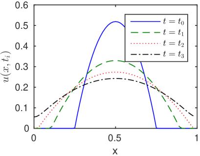
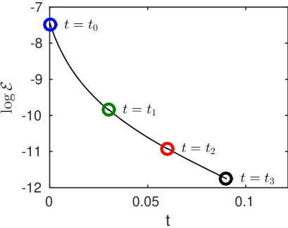
Figure 3. Left: Evolution of the intial datum (29) for $\beta=2$ at various time steps $t_{i}$, $i=0,1,2,3$. Right: Semi-logarithmic plot of the discrete entropy $H_{d}[u^{k}]$ versus time.

We set as before $u:=u^{k}$, $v(\tau):=u^{k-1}$ and compute $G(\tau)=H_{d}[u]-H_{d}[v(\tau)]$ and the discrete second-order derivative $\partial^{2}G$ of $G$ (using central differences). The result is presented in Figure 4. As expected, the discrete derivative $\partial^{2}G$ is negative on a (small) interval for all times $t_{i}$, $i=1,2,3$. We observe that $\partial^{2}G$ is even slightly decreasing, but we expect that it becomes positive for sufficiently large values of $\tau$. Clearly, the values for $\partial^{2}G$ tend to zero as we approach the steady state (see Remark 4). This experiment indicates that $\tau^{k}$ from Theorem 1 is bounded from below by $\tau^{*}=3\cdot 10^{-4}$, for instance.

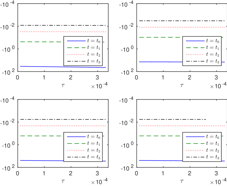
Figure 4. Numerical evaluation of the discrete version of $G^{\prime\prime}(\tau)$ for various Runge-Kutta schemes at the time steps $t_{i}$. Top left: explicit Euler scheme; top right: implicit Euler scheme; bottom left: implicit trapezoidal rule; bottom right: Simpson rule.

In order to understand the behavior of $G(\tau)$ in a better way, it is convenient to study the discrete version of the quotient

(30) $$Q(\tau):=\frac{G^{\prime\prime}(\tau)}{\|u^{\alpha+2\beta-2}u_{x}^{4}\|_{L^{1}}}.$$

Indeed, the analysis in Section 4 gives an estimate of the type $G^{\prime\prime}(0)\leq-C\int_{\Omega}u^{2\beta+\alpha-5}u_{x}^{4}dx$ for some constant $C>0$. Thus, we expect that for sufficiently small $\tau>0$, $Q(\tau)$ is bounded from above by some negative constant. This expectation is confirmed in Figure 5. In the examples, $Q(\tau)$ is a decreasing function of $\tau$, and $Q(0)$ is decreasing with increasing time.

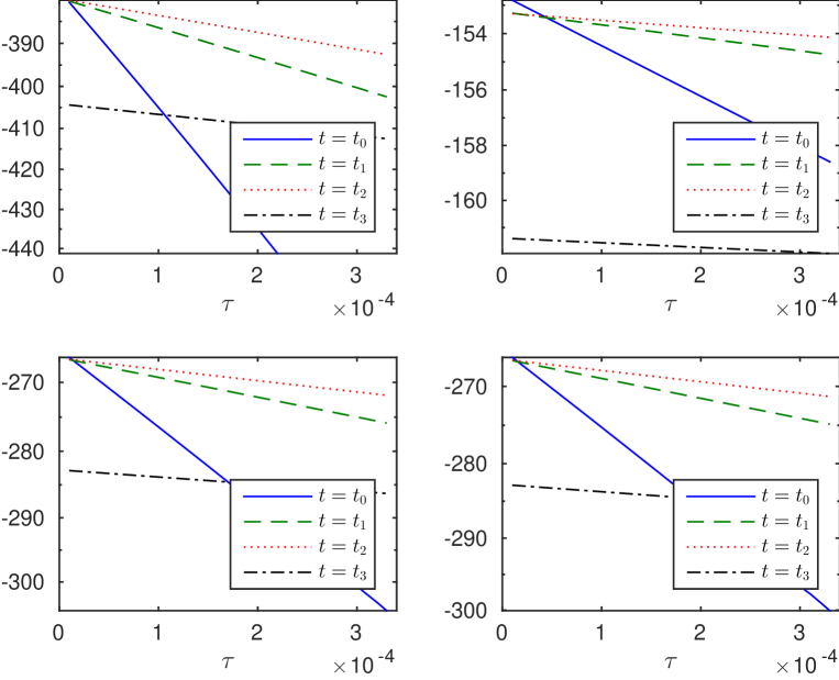
Figure 5. Numerical evaluation of the discrete version of $Q(\tau)$, defined in (30), for various Runge-Kutta schemes at the time steps $t_{i}$. Top left: explicit Euler scheme; top right: implicit Euler scheme; bottom left: implicit trapezoidal rule; bottom right: Simpson rule.

All these results indicate that the threshold parameter $\tau^{k}$ in Theorem 1 can be chosen independently of the time step $k$.

References

- [1] D. Bakry and M. Emery. Diffusions hypercontractives. In: Séminaire de probabilités XIX, 1983/84, Lect. Notes Math. 1123 (1985), 177-206.
- [2] M. Bessemoulin-Chatard. A finite volume scheme for convection-diffusion equations with nonlinear diffusion derived from the Scharfetter-Gummel scheme. Numer. Math. 121 (2012), 637-670.
- [3] S. Boscarino, F. Filbet, and G. Russo. High order semi-implicit schemes for time dependent partial differential equations. Preprint, 2015. https://hal.archives-ouvertes.fr/hal-00983924.
- [4] M. Bukal, E. Emmrich, and A. Jüngel. Entropy-stable and entropy-dissipative approximations of a fourth-order quantum diffusion equation. Numer. Math. 127 (2014), 365-396.
- [5] C. Cancès and C. Guichard. Numerical analysis of a robust entropy-diminishing finite-volume scheme for parabolic equations with gradient structure. Preprint, 2015. arXiv:1503.05649.
- [6] C. Chainais-Hillairet, A. Jüngel, and S. Schuchnigg. Entropy-dissipative discretization of nonlinear diffusion equations and discrete Beckner inequalities. To appear in ESAIM Math. Model. Numer. Anal., 2015. arXiv:1303.3791.
- [7] S. Christiansen, H. Munthe-Kaas, and B. Owren. Topics in structure-preserving discretization. Acta Numerica 20 (2011), 1-119.
- [8] K. Deimling. Nonlinear Functional Analysis. Springer, Berlin, 1985.
- [9] B. Derrida, J. Lebowitz, E. Speer, and H. Spohn. Fluctuations of a stationary nonequilibrium interface. Phys. Rev. Lett. 67 (1991), 165-168.
- [10] F. Filbet. An asymptotically stable scheme for diffusive coagulation-fragmentation models. Commun. Math. Sci. 6 (2008), 257-280.
- [11] A. Glitzky and K. Gärtner. Energy estimates for continuous and discretized electro-reaction-diffusion systems. Nonlin. Anal. 70 (2009), 788-805.
- [12] E. Hairer, S.P. Nørsett, and G. Wanner. Solving Ordinary Differential Equations I. Springer, Berlin, 1993.
- [13] A. Jüngel. Transport Equations for Semiuconductors. Lect. Notes Phys. 773, Springer, Berlin, 2009.
- [14] A. Jüngel and D. Matthes. An algorithmic construction of entropies in higher-order nonlinear PDEs. Nonlinearity 19 (2006), 633-659.
- [15] A. Jüngel and D. Matthes. The Derrida-Lebowitz-Speer-Spohn equation: existence, non-uniqueness, and decay rates of the solutions. SIAM J. Math. Anal. 39 (2008), 1996-2015.
- [16] A. Jüngel and J.-P. Milišić. A sixth-order nonlinear parabolic equation for quantum systems. SIAM J. Math. Anal. 41 (2009), 1472-1490.
- [17] A. Jüngel and J.-P. Milišić. Entropy dissipative one-leg multistep time approximations of nonlinear diffusive equations. To appear in Numer. Meth. Part. Diff. Eqs., 2015. arXiv:1311.7540.
- [18] M. Liero and A. Mielke. Gradient structures and geodesic convexity for reaction-diffusion systems. Phil. Trans. Royal Soc. A. 371 (2013), 20120346 (28 pages), 2013.
- [19] H. Liu and H. Yu. Entropy/energy stable schemes for evolutionary dispersal models. J. Comput. Phys. 256 (2014), 656-677.
- [20] E. Tadmor. Numerical viscosity of entropy stable schemes for systems of conservation laws I. Math. Comp. 49 (1987), 91-103.