Friction Causing Unpredictability

Abstract

The periodic motion of a classical point particle in a one-dimensional double-well potential acquires a surprising degree of complexity if friction is added. Finite uncertainty in the initial state can make it impossible to predict in which of the two wells the particle will finally settle. For two models of friction, we exhibit the structure of the basins of attraction in phase space which causes the final-state sensitivity. Adding friction to an integrable system with more than one stable equilibrium emerges as a possible “route to chaos” whenever initial conditions can be specified with finite accuracy only.

1 Introduction

The difficulty to reliably predict the behaviour of a classical systems is usually related to the existence of fractal structures in the mathematical model describing the system. Conservative non-integrable systems such as three interacting planetary bodies [1] and chaotic dissipative systems such as Lorenz’s model of the atmosphere [2] provide two well-known cases in point. Consider adding a third body to the integrable system of two planetary bodies which interact through gravitation. The KAM theorem [3] describes how the original foliation of the system’s phase-space into tori is being replaced gradually by a highly intricate mixed phase space. Finite balls of initial conditions will no longer contain trajectories on tori only but also others which separate at an exponential rate. The non-linearity present in Lorenz’s model gives rise to a strange attractor [4]. Its properties dominate the long-term evolution of the system since trajectories with neighboring initial conditions are likely to visit rather different regions of phase space at comparable later times. This phenomenon has been called final state sensitivity [5].

An actual macroscopic physical system, however, cannot exhibit fractal structures in a strict sense: the system would need to match its mathematical description on arbitrary length scales [6] but classical models break down on the molecular or atomic level. Experimentally observed structures may be highly intricate over many – but not all – orders of magnitude. Nevertheless, finite intricacies are sufficient to make reliable long-term predictions impossible when combined with initial states which are known only approximately.

Adding friction to conservative non-integrable model systems washes out fractal structures on the finest scales but remnants may continue to exist. This has been shown for a spherical pendulum with three stable equilibrium positions, in the presence of gravity [7]. When friction is added, basins of attraction with highly intricate boundaries emerge. If the initial state is not known exactly the fine structure of the basin boundaries – in spite of not being fractal – already prevents any reliable prediction of the equilibrium position near which the pendulum will come to rest.

The purpose of this paper is to identify a different mechanism which also results in an unpredictable final state if initial conditions are known only with finite accuracy. Starting from an integrable system with multiple stable equilibria, we will show that the addition of friction may create basins of attraction with intricate boundaries, leading to a situation which resembles the one of the pendulum just described. The main difference is that this mechanism does not rely on pre-existing fractal structures: instead, incorporating friction causes intricate structures to emerge in an originally integrable system.

Sec. 2 of this paper provides an initial, qualitative explanation of why adding friction to an integrable system with two or more stable equilibria may cause final-state sensitivity. Then, in Sec. 3, we investigate the structure of basins of attraction generated by two different types of friction when acting on a particle moving in a piece-wise constant double-well potential. Finally, we summarize and discuss our results in Sec. 4.

2 Final-state sensitivity in a double-well potential

To illustrate how friction creates final state sensitivity, we consider a classical particle moving along a straight line in the presence of a symmetric double-well potential. The system is described by the Hamiltonian function

$$H(p,q)=\frac{p^{2}}{2m}+W(q)\,,\quad p,q\in\mathbb{R\,},$$ (1)

where $q$ and $p$ denote position and the momentum of the particle, respectively. The minima of the potential $W(q)$ are located at $q=q_{\pm}$ , separated by a barrier of height $W_{0}\equiv W(0)$ which defines the critical energy, $E_{c}\equiv W_{0}$. The phase-space diagram of the system is shown in Fig. 1, displaying

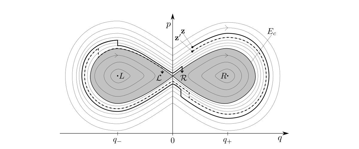
Figure 1: Phase-space structure of a double-well potential $W(q)$ with minima $L$ and $R$, located within wells ${\cal L}$ and ${\cal R}$ (shaded areas), respectively; a particle with neighbouring initial conditions $\mathbf{z},\mathbf{z}^{\prime}$ (full and dashed lines, respectively) may end up in different wells when subjected to periodic, dissipative “kicks” which reduce its momentum and thus its energy.

the familiar types of trajectories. The minima $L$ and $R$ of the potential are stable fixed points each surrounded by periodic orbits with energies $E$ not exceeding the critical value, $0<E<E_{c}\equiv W_{0}$. For $E=E_{c}$, the particle may rest at the unstable fixed point at $q=0$, or travel on one of the two separatrices connected to it. The trajectories with energy above the critical value, $E>E_{c}$ are periodic, encircling both minima on a single round trip. With a single degree of freedom and the energy $H(p,q)$ as a conserved quantity, the system is integrable, leading to the global foliation of its phase space into one-dimensional tori.

Adding friction will modify all trajectories except when then particle initially rests at one of the three fixed points. If located on a separatrix or on any periodic trajectory with energy less than $E_{c}$, dissipation will cause the particle to “spiral” into either the left or the right minimum of the potential $W(q)$, depending on its original position relative to the origin, $q=0$. The particle cannot escape from a well once it has been trapped, and the fixed points $L$ and $R$ turn into attractors.

The destiny of a particle with initial energy $E>E_{c},$ however, it is not immediately obvious since it may end up in either well. Friction will inevitably “draw” the particle towards the location of the separatrices of the unperturbed system. At some time, the energy of the particle will drop below the critical value $E_{c}$. The position of the particle relative to the origin at the time of the drop will determine whether it becomes trapped in the left or in the right well.

For simplicity, let us assume that friction acts at discrete times only, repeatedly reducing the momentum of the particle by a constant factor. Suppose that for initial conditions $\mathbf{z}=(p,q)^{T}$, the particle will – after a possibly long time – settle in the right well as illustrated in Fig. 1. Intuitively, a slightly smaller initial momentum (see $\mathbf{z}^{\prime}$ in the figure) could cause the particle to negotiate the barrier one less time and to settle in the left well instead. The slight change in the initial condition has thus altered the long-term behaviour of the system. Therefore, the finally state of a particle may become unpredictable from a practical point of view, i.e. whenever its initial conditions are known to lie within a small but finite volume of phase space only.

More formally, the non-Hamiltonian equations of motion map an initial state $\mathbf{z}(t_{0})$ to a new value $\mathbf{z}(t)$ at time $t$,

$$\mathbf{z}(t_{0})\mapsto\mathbf{z}(t),\quad\mathbf{z}\equiv\begin{pmatrix}p\\ q\end{pmatrix}\,,$$ (2)

leading to a decrease of the energy defined in (1): $E_{0}\to E<E_{0}$. To ascertain whether a particle with initial state $\mathbf{z}(t_{0})$ ends up near $L$ or near $R$, one needs to determine the earliest time $t$ such that its energy $E$ falls below the critical value,

$$E<E_{c}\,.$$ (3)

Repeating this calculation for all initial conditions will divide the phase space into two disjoint sets known as basins of attraction which encode whether the particle ends up in well ${\cal L}$ or ${\cal R}$. Let us investigate the structure of their boundaries for two models of friction, using a particularly simple double-well potential.

3 Piece-wise constant double-well potential with friction

The double-well potential considered here is based on a “particle in a box” defined by two infinitely high potential walls at $q=\pm\ell$ which restrict motion to a line segment of length $2\ell$. The particle bounces off the walls elastically resulting in an instantaneous reversal of its momentum: $p\to-p$; its position $q=\pm\ell$ remains unchanged when hitting a wall. A piece-wise constant potential,

$$W(q)=\begin{cases}W_{0}\,,&|q|<\varepsilon\,,\\ 0\,,&\varepsilon<|q|<\ell\,,\end{cases}$$ (4)

models the smooth double-well. For simplicity, we take an arbitrarily thin potential barrier, corresponding to $\varepsilon\to 0$. The only impact of this “infinitesimal” barrier is to confine the particle in a well once its energy drops below the critical value $W_{0}$, thus creating the wells ${\cal L}$ and ${\cal R}$. Two continuous sets of potential minima exist because the bottom of the potential is flat.

A widespread method to investigate non-integrable systems is to start with an integrable system and add a perturbation, be it a time-independent potential term as in the KAM theorem or a deterministic time-dependent force [8]. To support our claim that friction generically causes final state sensitivity, we will model it in two different ways which are inspired by these approaches. In the first case, the elastic collisions of the particle with the boundary walls are made inelastic (cf. Sec. 3.1) while an impulsive friction force is applied periodically in the second case (cf. Sec. 3.2). The first model depends on a single parameter only, the coefficient of restitution. The second model depends on two parameters, the frequency and the strength of the dissipative “kick.”

3.1 Inelastic collisions

The motion of the particle in the piece-wise constant double well (4) consists of free motion between the walls interspersed with momentum-reversing elastic collision at the walls. The dynamics changes fundamentally upon replacing the elastic collisions at the walls by inelastic ones, characterized by a coefficient of restitution, $r\in(0,1)$:

$$\mathbf{z}\mapsto\mathbf{z}^{\prime}=\mathbf{R\cdot}\mathbf{z}\text{\,,\quad$\mathbf{R}\equiv\left(\begin{array}[]{cc}-r&0\\ 0&1\end{array}\right)$\qquad for}\quad q=\pm\ell\,.$$ (5)

This minor change turns the conservative system into a dissipative one and – as we will see – is sufficient to create an embryonic form of final-state sensitivity.

The long-term dynamics of the particle does not depend on its initial position: all particles with fixed momentum $p_{0}$ but arbitrary position $q_{0}\in(-\ell,\ell)$ will experience the same amount of friction, only to end up in same well. Thus, let us assume that the particle starts out with positive initial momentum $p_{0}>p_{c}$, beings located at $q_{0}=\ell_{-}$, i.e. just to left of the right wall. Then, the initial state $\mathbf{z}_{0}=(p_{0},\ell_{-})$ at time $t_{0}$ evolves according to

$$\mathbf{z}(t_{n})=\mathbf{R}^{n}\cdot\mathbf{z}_{0}=\begin{pmatrix}(-r)^{n}p_{0}\\ \ell_{-}\end{pmatrix}\,,\qquad n\in\mathbb{N}_{0}\,,$$ (6)

with the times $t_{n}$ being defined by particle returning to its initial position $\ell_{-}$. Monitoring the value of its momentum at the walls is sufficient to determine the well which will trap the particle. The particle will be trapped in well ${\cal R}$, for example, if its last collision at the right wall makes its energy drop below the critical value $E=E_{c}$ due to $p\mapsto(-r)p$.

For positive initial momentum $p_{0}$ the particle will hit the right wall first. The well to finally trap the particle is determined by the number of collisions $n(E_{0})$ before it drops below $E_{c}$. Denoting the energy of the particle after $n$ collisions by $E_{n}$, we need to find the number $n(E_{0})$ such that the energy of the particle falls below $E_{c}$ for the first time,

$$n(E_{0})=\min_{n\in\mathbf{N}}\,\left\{E_{n}<E_{c}\right\}\,,\quad\mbox{with }E_{0}>E_{c}\,.$$ (7)

Using Eq. (6) the number $n(E_{0})$ is easily found to be

$$n(E_{0})=\left\lceil\frac{1}{2}\frac{\ln\left(E_{c}/E_{0}\right)}{\ln r}\right\rceil=\left\lceil\frac{\ln\left(p_{c}/p_{0}\right)}{\ln r}\right\rceil\,,$$ (8)

where the initial moment defines the initial energy, $E_{0}=p_{0}^{2}/2m$, and $\left\lceil x\right\rceil$ is the ceiling function extracting the smallest integer greater or equal to the number $x$. If $n$ is odd (even), a particle with positive momentum $p_{0}$ will end up in the well on the right (left). The basins of attraction for the wells ${\cal L}$ and ${\cal R}$ are given by alternating horizontal bands in phase space shown in Fig. 2. The widths of the bands decrease with decreasing friction (and they increase with energy $E$ which the figure does not show due to the limited momentum range).

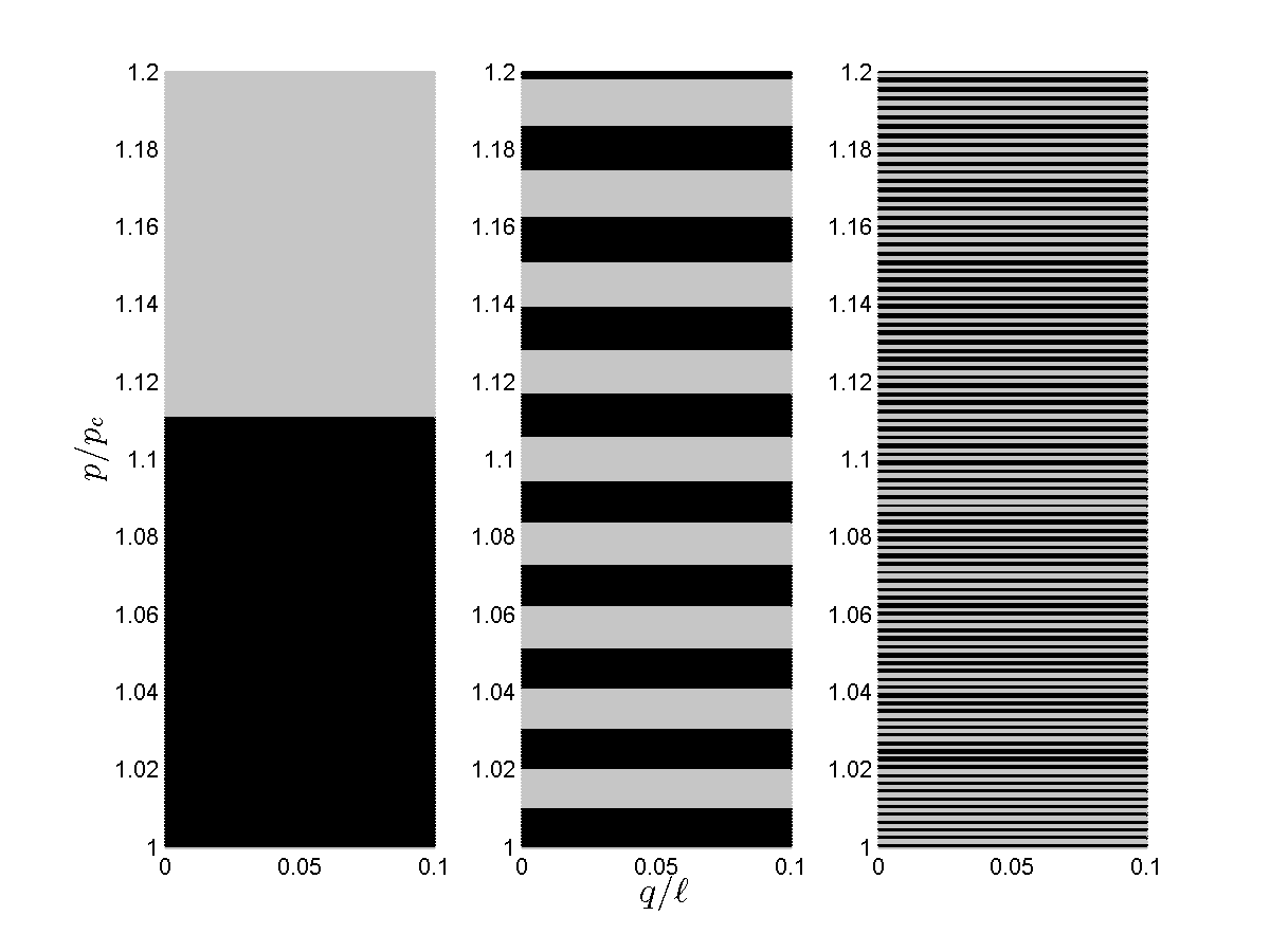
Figure 2: Basins of attraction for the phase-space region $(1\leq p/p_{c}\leq 1.2$, $0\leq q/\ell\leq 0.1$) of a particle of unit mass in a double-well, with friction arising from inelastic collisions at the boundary walls: initial conditions located in dark (light) regions will end up in the right (left) well of the potential. The vertical bars correspond to different values of the coefficient of restitution: $r=0.9$, $r=0.99$, $r=0.999$ (left to right). Smaller values of friction lead to increasing “complexity” of the basin boundaries, in the sense of producing narrower bands.

If the initial conditions $(p_{0},q_{0})$ of a particle are known exactly, then the deterministic dynamics leads to a unique and well-defined final state which can be predicted with certainty. However, limited precision of the initial conditions may results in a genuine indeterminacy of the final state. Assume that the initial state of the particle is only known to lie inside a rectangle with sides $\Delta q>0$ and $\Delta p>0$, centered about the point $\mathbf{z}_{0}$. Trajectories with initial momenta $p_{0}$ and $p_{0}^{\prime}\equiv rp_{0}$ are bound to end up in different wells. Thus, if the inaccuracy in momentum exceeds this value,

$$\Delta p>p_{0}-p_{0}^{\prime}\,,$$ (9)

the uncertainty rectangle will cut across at least two adjacent basins of attraction. In other words, given the initial momentum $p_{0}$ and any finite uncertainty $\Delta p$ about it, the prediction of the final state becomes impossible for a coefficient of restitution in the interval

$$1-\frac{\Delta p}{p_{0}}<r<1\,,$$ (10)

since the rectangle with sides $\Delta q$ and $\Delta p$ will contain trajectories destined for the wells ${\cal L}$ and ${\cal R}$. We conclude that sufficiently weak inelasticity prevents the reliable prediction of the final state. In this well-defined sense, adding friction to an integrable system provides a mechanism which prevents accurate long-term predictions.

3.2 Periodic damping

Now we turn to a model where friction is caused by a periodic, dissipative force which acts during a short time interval only. It will be convenient to consider the limit of an instantaneous action which multiplies the momentum of the particle by a constant factor $\gamma\in(0,1)$ at times $T_{k}=kT$, with $k\in\mathbb{N}$, and a free parameter $T$. This approach is analogous to periodically kicking a system with a deterministic force which, for a particle moving freely on a ring known as a “rotor,” produces deterministically chaotic motion [3]. Since our model depends on two independent parameters, $\gamma$ and $T$, we expect more complicated basins of attraction compared to the model with inelastic reflections.

To construct the basins of attraction of the wells ${\cal L}$ and ${\cal R}$, we need to determine when, for arbitrary initial conditions $(p_{0},q_{0})^{T}$, the energy of the particle falls below the critical value for the first time We then record whether, at that moment of time, it is located to the left or to the right of the origin, i.e. within ${\cal L}$ or ${\cal R}$. For simplicity, the particle is assumed to begin its journey at time $t=0^{+}$, i.e. just after $t=0$, with positive momentum $p_{0}>p_{c}$ and arbitrary initial position $q_{0}\in(-\ell,\ell$).

The particle moves freely during intervals of length $T$, with perfectly elastic collisions occurring at the boundary walls which only change the sign of its momentum. An expression for its time evolution in closed form can be found if we “unfold” the trajectory by imagining identical copies of the double-well to be arranged along the position axis. Instead of being reflected at the right wall located at $q=\ell$, the particle enters the next double well, which occupies the range $(\ell,3\ell$), and continues to move to the right, etc. In this setting, the momentum does not change its sign when the particle moves from one double well to the adjacent one. The sign of its momentum in the original double well is negative (or positive) if the particle has reached the $s^{th}$ copy of the double well, with $s\in\mathbb{N}$ being odd (or even).

To determine the dynamics of the system over one period of length $T$, we combine the free motion with the dissipative kicks:

1. during the motion of the particle from $t=0^{+}$ to just before the first kick at time $t=T$, its phase-space coordinates are given by

   $$\mathbf{z}(t)=\begin{pmatrix}p_{0}\\ q_{0}+p_{0}t/m\end{pmatrix}\equiv\mathbf{F}(t)\text{$\cdot$}\mathbf{z}_{0}\,,\qquad\mathbf{F}(t)=\begin{pmatrix}1&0\\ t/m&1\end{pmatrix}\,,\qquad t\in(0^{+},T^{-})\,,$$ (11)

   where $q\in(0,\infty)$ due to the unfolding;

2. the dissipative kick at time $T$ reduces the momentum of the particle by the factor $\gamma\in(0,1)$,

   $$\mathbf{z}(T^{+})=\begin{pmatrix}\gamma p(T^{-})\\ q(T^{-})\end{pmatrix}\mathbf{\equiv D}\cdot\mathbf{z}(T^{-})\,,\qquad\mathbf{D}=\left(\begin{array}[]{cc}\gamma&0\\ 0&1\end{array}\right)\,,\qquad t\in(T^{-},T^{+}).$$ (12)

To obtain the actual position and momentum of the particle inside the box at time $t$, we map (or “fold back”) the expression $\mathbf{F}(t)\cdot\mathbf{z}$ to the interval $q\in(-\ell,\ell)$, by writing

$$\mathbf{z}(t)=\begin{pmatrix}(-)^{s(t)}p_{0}\\ \left[\left(q_{0}+p_{0}t/m\right)\!\!\!\!\!\!\mod 2\ell\right]-\ell\end{pmatrix}\,,\qquad t\in(0^{+},T^{+})\,,$$ (13)

where the value of the integer $s(t)$ is determined by writing $q+pt/m=\overline{q}(t)+2\ell s$, with $\overline{q}(t)\in(-\ell,+\ell)$. The momentum $p$ changes sign whenever the “unfolded” coordinate passes through the values $\ell,3\ell,5\ell,\ldots$

The time evolution of the initial state $\mathbf{z}_{0}$ from time $t=0^{+}$ to $t=T_{k}^{+}\equiv(kT)^{+}$, i.e. just after the kick with label $k$, follows from concatenating Eqs. (11) and (12) $k$ times,

$$\mathbf{z}(T_{k}^{+})=\left(\mathbf{D}\cdot\mathbf{F}(T^{-})\right)^{k}\cdot\mathbf{z}_{0}\equiv\begin{pmatrix}\gamma&0\\ \gamma T/m&1\end{pmatrix}^{k}\cdot\mathbf{z}_{0}=\begin{pmatrix}\gamma^{k}&0\\ \sigma_{k}(\gamma)T/m&1\end{pmatrix}\cdot\mathbf{z}_{0}\,,$$ (14)

where

$$\sigma_{k}(\gamma)=\frac{1-\gamma^{k}}{1-\gamma}\,,\qquad k\in\mathbb{N}\,.$$ (15)

In analogy to Eq. (13), the “true” coordinates of the particle inside the box are obtained as

$$\mathbf{z}(T_{k}^{+})=\begin{pmatrix}(-)^{s(t)}\gamma^{k}p_{0}\\ \left[\left(q_{0}+\sigma_{k}(\gamma)p_{0}T/m\right)\mod 2\ell\right]-\ell\end{pmatrix}\,,$$ (16)

assuming that, after $k$ kicks, the energy $E_{k}=p_{k}^{2}/2m$ of the particle has not yet dropped below the critical value $E_{c}$.

We are now in the position to determine which initial conditions $\mathbf{z}_{0}$ will send the particle to the left and the right well, respectively. Using Eq. (16), we first determine the smallest value of $k$ which reduces the energy of the particle below the critical value, $E_{k}<E_{c}$, or

$$k_{c}=\left\lceil\frac{1}{2}\frac{\ln(E_{c}/E_{0})}{\ln\gamma}\right\rceil=\left\lceil\frac{\ln(p_{c}/p_{0})}{\ln\gamma}\right\rceil,\qquad k_{c}\in\mathbb{N}\,,$$ (17)

assuming, of course, that $p_{0}>p_{c}$. This relation structurally resembles the result (8), with the number $k_{c}$ of dissipative kicks playing the role of the number of inelastic collisions $n_{c}.$ The sign of the position coordinate after $k_{c}$ kicks, $q(T_{k_{c}}^{+})$, follows from Eq. (16) and determines whether the particle is trapped in ${\cal L}$ or ${\cal R}$. The explicit dependence of $\mathbf{z}(T_{k}^{+})$ on the initial position implies that changes in $q_{0}$ may also produce different final states, in contrast to the model studied in Sec. 3.1.

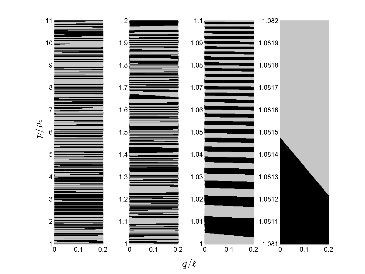
Figure 3: Basins of attraction for the phase-space region $(1\leq p/p_{c}\leq 11$, $0\leq q/\ell\leq 0.2$) of a particle with unit mass in a double-well, with friction arising from periodic dissipative kicks at times $kT$, $k\in\mathbb{N}$, with $\ell=1$, $T=100s$ and $\gamma=0.99$: initial conditions located in dark (light) regions will end up in the right (left) well of the potential. Each of the three vertical bars on the right magnifies a horizontal strip of the bar to its left by a factor of ten. The basin boundaries clearly exhibit both a momentum and a position dependence. Each bar results from iterating $501\times 501$ regularly spaced initial conditions inside the area shown.

Fig. 3, which has been generated numerically on the basis of Eq. (16), illustrates these conclusions. The first vertical bar visualizes the basins of attraction associated with the wells $\mathcal{L}$ and $\mathcal{R}$, respectively. The expected dependence on both initial momentum and position becomes clearly visible in the magnifications which also reveal that the boundaries of the apparently irregular basins of attractions are not fractal.

The boundaries of the basins can be found directly from Eq. (16): all initial conditions $(p_{0},q_{0})$ mapped to a fixed value of position at time $kT$ are located on lines of the form

$$p_{0}(q_{0})=-\frac{m}{\sigma_{k}(\gamma)T}q_{0}+\mbox{const}\simeq-\frac{1}{k}\frac{m}{T}q_{0}+\mbox{const}\,,\qquad\gamma\apprle 1\,,$$ (18)

using $\sigma_{k}(\gamma)\simeq(1/k)+{\cal O}(1-\gamma)$, which holds for weak damping, i.e. for $\gamma$ approaching the value one from below. Consequently, the boundaries of the basins of attraction are straight lines in phase space just as for the model with inelastic reflections off the wall. The lines are no longer horizontal but their slope approaches the value zero if a large number of kicks is required for the particle to settle in a well.

Assume once again that the initial conditions of the particle can be prepared with finite precision only, i.e. they lie inside a phase-space rectangle with area $\Delta q\Delta p>0$ and center $\mathbf{z}_{0}$. For any finite imprecision one can always find a damping strength $\gamma$ such that at least one basin boundary crosses the rectangle; this is sufficient to prevent the prediction of the well to finally trap the particle. For large initial momenta $p_{0}$, the reasoning behind the derivation of the inequality (10) also applies here since the strips constituting the basins of attraction will, typically, have almost horizontal boundaries. Thus, for any initial conditions $(p_{0},q_{0})$ and finite uncertainties, damping strengths within the interval

$$1-\frac{\Delta p}{p_{0}}<\gamma<1$$ (19)

correspond to a situation with an unpredictable final state. Occasionally, the uncertainty rectangle with sides $\Delta q$ and $\Delta p$ may cover an area where a slight change in initial position causes the particle to reach different wells, which only increases the final state sensitivity.

4 Summary and conclusions

We have shown that adding friction to an integrable one-dimensional double-potential well causes its dynamics to exhibit a rudimentary form of final-state sensitivity. For simplicity, the well has been modeled as a “box” divided into two regions by a thin wall. A particle has been subjected to two types of dissipative forces which, by reducing its initial energy, cause the particle to necessarily settle in one the wells after a finite, possibly long time. The main result of our study is that adding friction to an integrable system produces basins of attraction with finely structured boundaries.

If the particle collides inelastically with the confining walls the resulting basins foliate the phase space of the system into horizontal layers of variable width which get narrower for decreasing friction. Any ball of initial conditions which extends beyond more than one band prevents us from predicting with certainty the well in which the particle will finally settle. Periodic dissipative kicks create basins of attraction with slightly more intricate boundaries, due to their additional position dependence. Since the particle must settle in a well after finite time the observed structures cannot be fractal. In practice, however, it is crucial whether the initial conditions can be specified with sufficient accuracy to avoid a spread across basins which send the particle to different final states.

These model systems demonstrate that adding friction to an integrable system with multiple stable equilibria can have a fundamental impact on long-term predictability. The motion is not “deterministically random” which would require fractal phase-space structures. However, if the accuracy of the initial conditions falls below a specific threshold, the final state of the system cannot be predicted reliably. Experimentally, the precision required for a reliable long-term prediction may well be out of reach.

We expect our conclusions to be structurally stable in the sense that they should not depend on the model of friction used. Any dissipative mechanism will, firstly, contract all initial conditions into a small phase-space region which is energetically just above the barrier of the double well; secondly, the energy of the particle will drop below $E_{c}$ in a way which depends sensitively on the initial conditions. Continuous Stokes friction, for example, is thus likely to generate similar basins of attraction.

To systematically study the creation of basins of attraction with intricate boundaries in more general, smooth potential wells, we suggest to exploit the existence of action-angle variables $(I,\varphi)$ in integrable systems. The energy $E$ represents a convenient starting point to study the impact of friction forces, when expressed as a function of the action $I$,

$$I(E)=\oint p(q,E)dq\,.$$ (20)

Suitable perturbations are easily added to the new form of the Hamiltonian, $H=H(I)$, once position $q$ and momentum $p$ have been mapped to $(I,\varphi$) by means of a canonical transformation.

Finally, we highlight a natural application of the effective unpredictability of a final state due to friction, given sufficiently imprecise initial conditions. It arises upon introducing a larger number of identical potential wells arranged on a ring, (37 or 38, say), mimicking a one-dimensional roulette wheel. Including periodic dissipative kicks provides a surprisingly simple explanation why a finite spread in initial momenta and positions is sufficient to generate random outcomes, the working hypothesis underlying any gambling. This approach should be contrasted with models of an actual roulette wheel where unpredictable trajectories arise through a multitude of effects: motion in a bent annulus-shaped region embedded into three dimensions, the presence of gravity, rolling resistance and a (presumably) non-integrable time-dependent potential.

Acknowledgments

JO is grateful for financial support through a “Summer-2014 Publication Studentship”, provided by the Department of Mathematics at the University of York, UK.

References

- [1] H. Poincaré: Les méthodes nouvelles de la mécanique céleste, Vols. I-III. Gauthier-Villars et fils, Paris (1899)
- [2] E. N. Lorenz: Deterministic Nonperiodic Flow. J. Atmos. Sci. 20, 130–141 (1963)
- [3] V. I. Arnol’d: Mathematical Methods of Classical Mechanics. Springer Science & Business Media New York (1989)
- [4] D. Ruelle, F. Takens: On the Nature of Turbulence. Comm. Math. Phys. 20, 167–192 (1971)
- [5] C. Grebogi, S. W. McDonald, E. Ott, J. A. Yorke: Final State Sensitivity: An Obstruction to Predictability. Phys. Lett. A 99, 415-418 (1983)
- [6] B. Mandlbrot: Fractals: Form, Chance and Dimension. Freeman, San Francisco, CA (1977)
- [7] A. Motter, M. Gruiz, G. Karolyi, T. Tel: Doubly Transient Chaos: The Generic Form of Chaos in Autonomous Dissipative Systems. Phys. Rev. Lett. 111, 194101 (2013)
- [8] B. V. Chirikov: A Universal Instability of Many-Dimensional Oscillator Systems. Phys. Rep. 52, 263 (1979)