Abstract
The present work deals with the resolution of the Poisson equation in a bounded domain made of a thin and periodic layer of finite length placed into a homogeneous medium. We provide and justify a high order asymptotic expansion which takes into account the boundary layer effect occurring in the vicinity of the periodic layer as well as the corner singularities appearing in the neighborhood of the extremities of the layer. Our approach combines the method of matched asymptotic expansions and the method of periodic surface homogenization, and a complete justification is included in the paper or its appendix.

Keywords
asymptotic analysis, periodic surface homogenization, singular asymptotic expansions.

Introduction

The present work is dedicated to the construction of a high order asymptotic expansion of the solution to a Poisson problem posed in a polygonal domain which excludes a set of similar small obstacles equi-spaced along the line between two re-entrant corners. The distance between two consecutive obstacles, which appear to be holes in the domain, and the diameter of the obstacles are of the same order of magnitude $\delta$, which is supposed to be small compared to the dimensions of the domain. The presence of this thin periodic layer of holes is responsible for the appearance of two different kinds of singular behaviors. First, a highly oscillatory boundary layer appears in the vicinity of the periodic layer. Strongly localized, it decays exponentially fast as the distance to the periodic layer increases. Additionaly, since the thin periodic layer has a finite length and ends in corners of the boundary, corners singularities come up in the neighborhood of its extremities. The objective of this work is to provide a sophisticated asymptotic expansion that takes into account these two types of singular behaviors.

The boundary layer effect occurring in the vicinity of the periodic layer is well-known. It can be described using a two-scale asymptotic expansion (inspired by the periodic homogenization theory) that superposes slowly varying macroscopic terms and periodic correctors that have a two-scale behavior: these functions are the combination of highly oscillatory and decaying functions (periodic of period $\delta$ with respect to the tangential direction of the periodic interface and exponentially decaying with respect to $d/\delta$, $d$ denoting the distance to the periodic interface) multiplied by slowly varying functions. This boundary layer effect has been widely investigated since the work of Sanchez-Palencia [37, 36], Achdou [2, 3] and Artola-Cessenat [5, 6]. In particular, high order asymptotics have been derived in [4, 27, 13, 9] for the Laplace equation and in [34, 35] for the Helmholtz equation.

On the other hand, corner singularities appearing when dealing with singularly perturbed boundaries have also been widely investigated. Among the numerous examples of such singularly perturbed problems, we can mention the cases of small inclusions (see [29, chapter 2] for the case of one inclusion and [8] for the case of several inclusions), perturbed corners [16], propagation of waves in thin slots [23, 24], the diffraction by wires [14], or the mathematical investigation of patched antennas [7]. Again, this effect can be depicted using two-scale asymptotic expansion methods that are the method of multiscale expansion (sometimes called compound method) and the method of matched asymptotic expansions (see [38, 29, 22]). Following these methods, the solution of the perturbed problem may be seen as the superposition of slowly varying macroscopic terms that do not see directly the perturbation and microscopic terms that take into account the local perturbation.

Recently, Vial and co-authors [39, 11] investigated a Poisson problem in a polygonal domain surrounded by a thin and homogeneous layer, while Nazarov [31] studied the resolution of a general elliptic problem in a polygonal domain with periodically changing boundary. In their studies they have combined the two different kinds of asymptotic expansions mentioned above in order to deal with both corner singularities and the boundary layer effect. Based on the multiscale method, the authors of [39, 11] constructed and justified a complete asymptotic expansion for the case of the homogeneous layer. For the periodic boundary in [31] the first terms of the asymptotic expansion have been constructed and error estimates have been carried out. This asymptotic expansion relies on a sophisticated analysis of solution behavior at infinity for the Poisson problem in an infinite cone with oscillating boundary with Dirichlet boundary conditions by Nazarov [30], where he published an analysis for Neumann boundary conditions in [32]. In the present paper, we are going to extend the work for the homogeneous layer and the periodic boundary by constructing explicitely and rigorously justifying asymptotic expansion for the above mentioned periodic layer transmission problem to any order (with Neumann boundary conditions on the perforations of the layer).

1 Description of the problem and main results

1.1 Description of the problem

In this section we are going to define the domain of interest $\Omega^{\delta}\in{\mathbb{R}}^{2}$, its limit when $\delta\to 0$ and the problem considered. With the coordinates $\mathbf{x}=(x_{1},x_{2})$ of ${\mathbb{R}}^{2}$ let $\Omega_{\mathrm{B}}$ and $\Omega_{\mathrm{T}}$ be the two adjacent rectangular domains defined by

$$\Omega_{\mathrm{B}} =(-L,L)\times(-H_{B},0)\ , \Omega_{\mathrm{T}} =(-L^{\prime},L^{\prime})\times(0,H_{\mathrm{T}})\ ,$$

where $L^{\prime}>L$, $H_{\mathrm{B}}$ and $H_{\mathrm{T}}$ are positive numbers. We denote by $\Gamma$ the common interface of $\Omega_{\mathrm{B}}$ and $\Omega_{\mathrm{T}}$, i. e.,

$$\overline{\Gamma}=\overline{\partial\Omega_{\mathrm{B}}}\cap\overline{\partial\Omega_{\mathrm{T}}}\quad\text{and}\quad\Gamma=(-L,L)\times\{0\}.$$

and we consider the (non-convex) polygonal domain (see Fig. 1(a))

$$\Omega=\Omega_{\mathrm{B}}\cup\Omega_{\mathrm{T}}\cup\Gamma\ ,$$

which has two reentrant corners at $\mathbf{x}_{O}^{\pm}=(\pm L,0)$ with both an angle of $\frac{3\pi}{2}$.

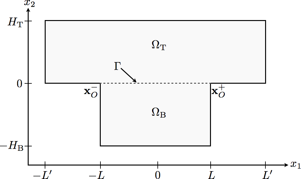
(a) The domain $\Omega=\Omega_{\mathrm{T}}\cap\Omega_{\mathrm{B}}\cap\Gamma$.

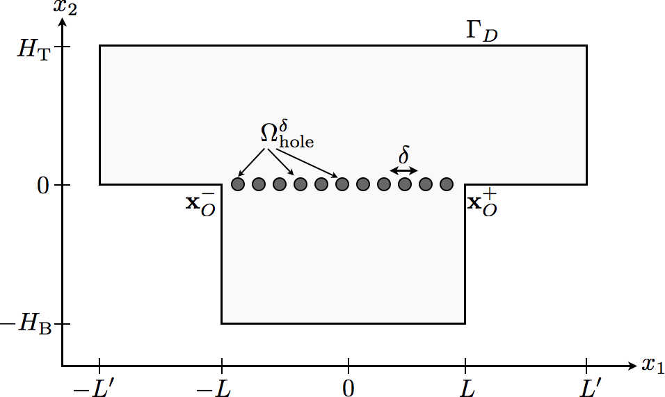
(b) The domain of interest $\Omega^{\delta}=\Omega\backslash\overline{\Omega^{\delta}_{\text{\rm hole}}}$.

Figure 1: Illustration of the polygonal domain $\Omega$ and the domain of interest $\Omega^{\delta}$.

Besides, let $\widehat{\Omega}_{\text{\rm hole}}\in{\mathbb{R}}^{2}$ be a smooth canonical bounded open set (not necessarily connected) strictly included in the domain $(0,1)\times(-1,1)$. Then, let $N^{\ast}:=\mathbb{N}\setminus\{0\}$ denote the set of positive integers and let $\delta$ be a positive real number (that is supposed to be small) such that

$$\frac{2L}{\delta}=q\in\mathbb{N}^{\ast}.$$ (1.1)

Now, let $\Omega^{\delta}_{\text{\rm hole}}$ be a thin (periodic) layer consisting of $q$ equi-spaced similar obstacles which can be defined by scaling and shifting the canonical obstacle $\widehat{\Omega}_{\text{\rm hole}}$ (see Fig. 1(b)):

$$\Omega^{\delta}_{\text{\rm hole}}=\bigcup_{\ell=1}^{q}\left\{-L\mathrm{e}_{1}+\delta\{\widehat{\Omega}_{\text{\rm hole}}+(\ell-1)\mathrm{e}_{1}\}\,\right\}.$$ (1.2)

Here, $\mathrm{e}_{1}$ and $\mathrm{e}_{2}$ denote the unit vectors of ${\mathbb{R}}^{2}$ and $\delta$ is assumed to be smaller than $H_{\mathrm{T}}$ and $H_{\mathrm{B}}$ such that $\Omega^{\delta}_{\text{\rm hole}}$ does not touch the top or bottom boundaries of $\Omega$. Finally, we define our domain of interest as

$$\Omega^{\delta}=(\Omega_{\mathrm{B}}\cup\Omega_{\mathrm{T}}\cup\Gamma)\backslash\overline{\Omega^{\delta}_{\text{\rm hole}}}.$$

Its boundary $\partial\Omega^{\delta}$ consists of the boundary of the set of holes $\Gamma^{\delta}=\partial\Omega^{\delta}_{\text{\rm hole}}$ and $\Gamma_{D}=\partial\Omega^{\delta}\setminus\Gamma^{\delta}=\partial\Omega$, the boundary of $\Omega$. Here and in what follows, we denote by ${\mathbf{n}}$ the outward unit normal vector of $\partial\Omega^{\delta}$. Note, that in the limit $\delta\to 0$ the repetition of holes degenerates to the interface $\Gamma$, the domain $\Omega^{\delta}$ to the domain $\Omega_{\mathrm{T}}\cup\Omega_{\mathrm{B}}$ and its boundary $\partial\Omega^{\delta}$ to $\partial\Omega\cup\Gamma$.

The domain $\Omega^{\delta}$ being defined, we can introduce the problem to be considered in this article: Seek $u^{\delta}$ solution to

$$\left\{\quad\begin{aligned} -\Delta u^{\delta}&=f,&\quad&\text{in }\Omega^{\delta}\ ,\\ \nabla u^{\delta}\cdot{\mathbf{n}}&=0,&&\text{on }\Gamma^{\delta},\\ u^{\delta}&=0,&&\text{on }\Gamma_{D}\ ,\end{aligned}\right.$$ (1.3)

where $f\in L^{2}(\Omega^{\delta})$. It is natural to search for $u^{\delta}\in\mathrm{H}^{1}_{\Gamma_{D}}(\Omega^{\delta})$ where

$$\mathrm{H}^{1}_{\Gamma_{D}}(\Omega^{\delta})=\left\{u\in H^{1}(\Omega^{\delta})\;\mbox{such that}\;u=0\;\mbox{on}\;\Gamma_{D}\right\}.$$ (1.4)

The well-posedness of problem (1.3) in $\mathrm{H}^{1}_{\Gamma_{D}}(\Omega^{\delta})$ directly follows from Lax-Milgram theorem:

Proposition 1.1 (Existence, uniqueness and stability).

Let $f\in L^{2}(\Omega^{\delta})$. Then, for any $\delta>0$ there exists a unique solution $u^{\delta}$ of problem (1.3) in $\mathrm{H}^{1}_{\Gamma_{D}}(\Omega^{\delta})$, and with a constant $C$ (independent of $\delta$) it holds

$$\left\lVert u^{\delta}\right\rVert_{\mathrm{H}^{1}(\Omega^{\delta})}\leqslant C\,\left\lVert f\right\rVert_{\mathrm{L}^{2}(\Omega^{\delta})}\,.$$ (1.5)

The objective of this paper is to describe the behavior of $u^{\delta}$ as $\delta$ tends to $0$. For the sake of simplicity, we shall assume that $f$ has a compact support in a subset of $\Omega_{\mathrm{T}}$ with distance $\delta_{0}>0$ to $\Gamma$. Our work relies on a construction of an asymptotic expansion of $u^{\delta}$ as $\delta$ tends to $0$.

Remark 1.2.

The construction is for simplicity for the specific geometrical setting, where $\Gamma$ is a straight line ending in two corners of the polygonal boundary $\partial\Omega$, where the angles between $\Gamma$ and $\partial\Omega$ are both ends at angles $\frac{\pi}{2}$ or $\pi$, respectively. Nevertheless, the study may be extended to a polygon $\Omega$ of different angles.

Remark 1.3.

It is worth noting that the choice of the boundary condition imposed on the small obstacles $\Gamma^{\delta}$ constituting the periodic layer, here homogeneous Neumann boundary conditions, has a strong impact on the asymptotic expansion. A homogeneous Dirchlet condition would yield to a completely different asymptotic expansion (see for instance Appendix A in [17], or [12]).

Remark 1.4.

The smoothness of $\widehat{\Omega}_{\text{\rm hole}}$ is not required for the existence of $u^{\delta}\in H^{1}(\Omega^{\delta})$. The well-posedness result remains valid if $\widehat{\Omega}_{\text{\rm hole}}$ is a Lipschitz domain. However, we use this assumption in the forthcoming analysis (In particular in Proposition 4.5 and Section 6).

1.2 Ansatz of the asymptotic expansion

As mentioned in the introduction, due to the periodic layer, it seems not possible to write a simple asymptotic expansion valid in the whole domain. We have to take into account both the boundary layer effect in the vicinity of $\Gamma$ and the additional corner singularities appearing in the neighborhood of the two reentrant corners. To do so, we shall distinguish a far field area located ’ far’ from the reentrant corners $\mathbf{x}_{O}^{\pm}$ and two near field zones located in the vicinity of them (see Fig. 2).

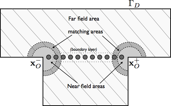
Figure 2: Schematic representation of the overlapping subdomains for the asymptotic expansion. The far field area (hatched) away from the corners $\mathbf{x}_{O}^{\pm}$ is overlapping the near field area (light grey) in the matching zone (dark grey).

1.2.1 Far field expansion

Far from the two corners $\mathbf{x}_{O}^{\pm}$ (hatched area in Fig. 2), we shall see that $u^{\delta}$ is the superposition of a macroscopic part (that is not oscillatory) and a boundary layer localized in the neighborhood of the thin periodic layer. More precisely, we choose the following ansatz:

$$u^{\delta}(\mathbf{x})=\sum_{(n,q)\in\mathbb{N}^{2}}\delta^{\frac{2}{3}n+q}\,u_{FF,n,q}^{\delta}(\mathbf{x}),$$ (1.6)

where $\mathbf{x}=(x_{1},x_{2})$, and for $(n,q)\in\mathbb{N}^{2}$

$$u_{FF,n,q}^{\delta}(\mathbf{x})=\begin{cases}u_{n,q}^{\delta}(\mathbf{x})&\mbox{if}\;|x_{1}|>L,\\[4.30554pt] \chi\left(\frac{x_{2}}{\delta}\right)u_{n,q}^{\delta}(\mathbf{x})+\Pi_{n,q}^{\delta}(x_{1},\frac{\mathbf{x}}{\delta})&\mbox{if}\;|x_{1}|<L.\end{cases}$$ (1.7)

Here $\chi:\mathbb{R}\mapsto(0,1)$ denotes a smooth cut-off function satisfying

$$\chi(t)=\begin{cases}1&\mbox{if}\;|t|>2,\\[4.30554pt] 0&\mbox{if}\;|t|<1.\end{cases}$$ (1.8)

The macroscopic terms $u_{n,q}^{\delta}$ are defined in the limit domain $\Omega_{\mathrm{T}}\cup\Omega_{\mathrm{B}}$. A priori, they are not continuous across $\Gamma$. As for the boundary layer correctors $\Pi_{n,q}^{\delta}(x_{1},X_{1},X_{2})$ (also sometimes denoted periodic correctors), and as usual in the periodic homogenization theory, there are $1$-periodic with respect to the scaled tangential variable $X_{1}$. Consequently, they are defined in $(-L,L)\times\mathcal{B}$, where $\mathcal{B}$ is the infinite periodicity cell (see Fig. 3(a)):

$$\mathcal{B}=\left\{(0,1)\times\mathbb{R}\right\}\setminus\overline{\widehat{\Omega}_{\text{\rm hole}}}.$$ (1.9)

Moreover, the periodic correctors are super-algebraically decaying as the scaled variable $X_{2}$ tends to $\pm\infty$ (they decay faster than any power of $X_{2}$), more precisely, for any $(k,\ell)\in\mathbb{N}^{2}$,

$$\lim_{|X_{2}|\rightarrow+\infty}X_{2}^{k}\partial_{X_{2}}^{\ell}\Pi_{n,q}^{\delta}=0.$$ (1.10)

The macroscopic terms as well as the boundary layer corrector terms might have a polynomial dependence with respect to $\ln\delta$: there is $N(n,q)\in\mathbb{N}$ such that

$$u_{n,q}^{\delta}=\sum_{s=0}^{N(n,q)}(\ln\delta)^{s}\,u_{n,q,s},\quad\mbox{and}\quad\Pi_{n,q}^{\delta}=\sum_{s=0}^{N(n,q)}(\ln\delta)^{s}\Pi_{n,q,s},$$

where $u_{n,q,s}$ and $\Pi_{n,q,s}$ do not depend on $\delta$.

Remark 1.5.

Here and in what follows, although it might be surprising at first glance, we call far field expansion the expansion (1.6), i. e., the superposition of the macroscopic terms and the boundary layer correctors. Besides, it should also be noted that, for any $k\in\mathbb{N}$, we consider $\delta^{\frac{2(n+3k)}{3}+q}$ and $\delta^{\frac{2n}{3}+(q+2k)}$ as different scales as they would be different powers of $\delta$. In fact, we shall see that $n$ and $q$ play a different role in the asymptotic procedure. Finally, following Remark 1.2, the consideration of the more general case of two angles of measure $\alpha$, would yield to an expansion of the form  (1.6) substituting $\delta^{\frac{2n}{3}+q}$ for $\delta^{\frac{\pi n}{\alpha}+q}$ (see [11]).

1.2.2 Near field expansions

In the vicinity of the two corners $\mathbf{x}_{O}^{\pm}$ (light grey areas in Fig. 2), the solution varies rapidly in all directions. Therefore, we shall see that

$$u^{\delta}(\mathbf{x})=\sum_{(n,q)\in\mathbb{N}^{2}}\delta^{\frac{2n}{3}+q\,}U_{n,q,\pm}^{\delta}\left(\frac{\mathbf{x}-\mathbf{x}_{O}^{\pm}}{\delta}\right)\,,$$ (1.11)

for some near field terms $U_{n,q,\pm}^{\delta}$ defined in the fixed unbounded domains

$$\widehat{\Omega}^{-}=\mathcal{K}^{-}\setminus\bigcup_{\ell\in\mathbb{N}}\left\{\overline{\widehat{\Omega}_{\text{\rm hole}}}+\ell\mathbf{e}_{1}\right\},\quad\widehat{\Omega}^{+}=\mathcal{K}^{+}\setminus\bigcup_{\ell\in\mathbb{N}^{\ast}}\left\{\overline{\widehat{\Omega}_{\text{\rm hole}}}-\ell\mathbf{e}_{1}\right\}$$ (1.12)

shown in Figure 3(b) and 3(c), where $\mathcal{K}^{\pm}$ are the unbounded angular domains

$$\mathcal{K}^{\pm} =\left\{\mathbf{X}=R^{\pm}(\cos\theta^{\pm},\sin\theta^{\pm}),R^{\pm}\in\mathbb{R}^{\ast}_{+},\theta^{\pm}\in I^{\pm}\right\}\in\mathbb{R}^{2}$$

of angular sectors $I^{+}=(0,\frac{3\pi}{2})$ and $I^{-}=(-\frac{\pi}{2},\pi)$. If the domain $\widehat{\Omega}_{\text{\rm hole}}$ is symmetric with respect to the axis $X_{1}=1/2$, then the domain $\widehat{\Omega}^{-}$ is nothing but the domain $\widehat{\Omega}^{+}$ mirrored with respect to the axis $X_{1}=0$. However, this is not the case in general. Similarly to the far field terms the near field terms might also have a polynomial dependence with respect to $\ln\delta$, i. e., for all $(n,q)\in\mathbb{N}^{2}$, there is $N(n,q)\in\mathbb{N}$ such that

$$U_{n,q,\pm}^{\delta}=\sum_{s=0}^{N(n,q)}(\ln\delta)^{s}U_{n,q,\pm,s}\ ,$$

where the functions $U_{n,q,\pm,s}$ do not depend on $\delta$.

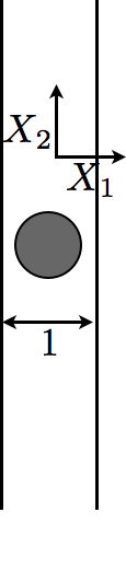
(a) The periodicity cell $\mathcal{B}$.

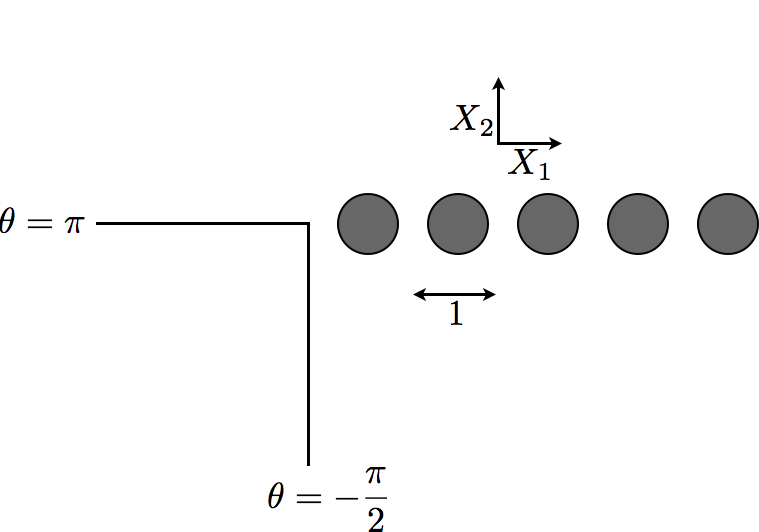
(b) The domain $\widehat{\Omega}^{-}$.

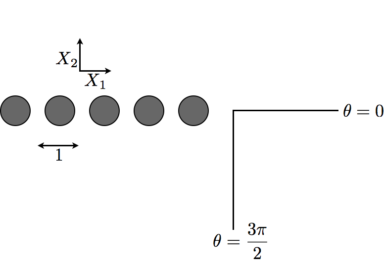
(c) The domain $\widehat{\Omega}^{+}$.

Figure 3: The periodicity cell $\mathcal{B}$ and the normalized domains $\widehat{\Omega}^{\pm}$.

1.2.3 Matching principle

To link the two different expansions, we assume that they are both valid in two intermediate areas ${\Omega}^{\delta,\pm}_{\mathcal{M}}$ (dark shaded in Fig. 2) of the following form:

$${\Omega}^{\delta,\pm}_{\mathcal{M}}=\left\{\mathbf{x}=(x_{1},x_{2})\in\Omega,\sqrt{\delta}\leq d(\mathbf{x},\mathbf{x}_{O}^{\pm})\leq 2\,\sqrt{\delta}\right\},$$

where $d$ denotes the usual Euclidian distance. The precise definition of the matching areas is not important. The reader might just keep in mind that they correspond to a neighborhood of the corners $\mathbf{x}_{O}^{\pm}$ of the reentrant corners for the far field terms (macroscopic and boundary layer correctors) and to $R^{\pm}$ going to $+\infty$ for the near field terms (expressed in the scaled variables).

1.3 Far and near field equations

The ’ansatz’ being assumed, the next objective is to construct the terms $u_{n,q}^{\delta}$, $\Pi_{n,q}^{\delta}$ and $U_{n,q,\pm}^{\delta}$ of the far and near field expansions (the asymptotic expansions are justified later, by proving error estimates). This is by far the longest part of the work (Sections 1 to 5). The usual starting point of this construction consists in the formal derivation of the near field and far field problems, that is to say problems satisfied by the near and far field terms.

1.3.1 Far field equations: macroscopic and boundary layer correctors equations

Inserting the far field expansion into the initial problem (1.3) and separating the different powers of $\delta$ (the complete procedure, based on the separation of the scales, is explained in Appendix A) gives a collection of equations for the macroscopic terms and the boundary layer terms:

Macroscopic equations

The macroscopic terms $u_{n,q}^{\delta}$ satisfy

$$-\Delta u_{n,q}^{\delta}=\begin{cases}f\;&\mbox{if}\;n=q=0,\\ 0\;&\mbox{otherwise,}\end{cases}\mbox{in}\;\Omega_{\mathrm{T}}\cup\Omega_{\mathrm{B}},$$ (1.13)

together with homogeneous Dirichlet boundary conditions on $\Gamma_{D}$

$$u_{n,q}^{\delta}=0\;\mbox{on}\;\,\Gamma_{D}.\\$$ (1.14)

Boundary layer corrector equations

The boundary layer correctors satisfy

$$\left\{\begin{aligned} -\Delta_{{\mathbf{X}}}\Pi_{n,q}^{\delta}(x_{1},{\mathbf{X}})&=&G_{n,q}^{\delta}&\quad\mbox{in}\;\mathcal{B},\\ \partial_{n}\Pi_{n,q}^{\delta}&=&\;\;0&\quad\mbox{on}\;\partial\widehat{\Omega}_{\text{\rm hole}}.\end{aligned}\right.$$ (1.15)

where, for any $p\in\mathbb{N}$,

$$G_{n,q}^{\delta}=\sum_{p=0}^{q}\frac{\partial^{p}u_{n,q-p}^{\delta}}{{\partial x_{2}}^{p}}(x_{1},0^{+})[\Delta,\chi_{+}]\left(\frac{(X_{2})^{p}}{p!}\right)+\sum_{p=0}^{q}\frac{\partial^{p}u_{n,q-p}^{\delta}}{{\partial x_{2}}^{p}}(x_{1},0^{-})[\Delta,\chi_{-}]\left(\frac{(X_{2})^{p}}{p!}\right)\\ +\partial_{x_{1}}^{2}\Pi_{n,q-2}^{\delta}(x_{1},{\mathbf{X}})+2\partial_{x_{1}}\partial_{X_{1}}\Pi_{n,q-1}^{\delta}(x_{1},{\mathbf{X}}).$$ (1.16)

Here, for any sufficiently smooth function $v$, $[\Delta,v]$ denotes the commutator between $\Delta$ and $v$, that is to say

$$[\Delta,v]u=\Delta(vu)-v\Delta u=\nabla v\cdot\nabla u+u\Delta v.$$

Moreover, the smooth truncation functions $\chi_{\pm}$ are defined by

$$\chi_{\pm}(X_{2})=\begin{cases}\,\chi(X_{2}),&\mbox{if}\pm X_{2}>0,\\ 0&\mbox{otherwise},\end{cases}\qquad(\chi_{\pm}(X_{2})=1_{(\pm X_{2}>0)}\chi(X_{2})),$$ (1.17)

and, for $p\in\mathbb{N}$,

$$\frac{\partial^{p}u_{n,q-p}^{\delta}}{{\partial x_{2}}^{p}}(x_{1},0^{\pm})=\lim_{h\rightarrow 0^{\pm}}\frac{\partial^{p}u_{n,q-p}^{\delta}}{{\partial x_{2}}^{p}}(x_{1},h).$$

Note that equations (1.13-1.14), posed in the domains $\Omega_{\mathrm{T}}$ and $\Omega_{\mathrm{B}}$, do not define entirely the macroscopic terms. Indeed, we first have to prescribe transmission conditions across the interface $\Gamma$ (for instance the jump of their trace and the jump of their normal trace across $\Gamma$). This information will appear to be a consequence of the boundary layer equations (Section 2). Then, we also have to prescribe the behavior of the macroscopic terms in the vicinity of the two corner points $\mathbf{x}_{O}^{\pm}$. This information will be provided by the matching conditions (Section 5).

1.3.2 Near field equations

The near field equations are obtained in a much more direct way. Inserting the near field ansatz (1.11) into the Laplace equation (1.3) and separating formally the different powers of $\delta$, it is easily seen that the near field term $U_{n,q}^{\delta}$ satisfy

$$\left\{\begin{aligned} -\Delta_{\mathbf{X}}U_{n,q}^{\delta}&=&0&\quad\mbox{in}\;\widehat{\Omega}^{\pm},\\ U_{n,q}^{\delta}&=&0&\quad\mbox{on}\;\partial\mathcal{K}^{\pm},\\ \partial_{n}U_{n,q}^{\delta}&=&0&\quad\mbox{on}\,\partial\widehat{\Omega}^{\pm}_{\text{\rm hole}}=\partial\widehat{\Omega}^{\pm}\setminus\partial\mathcal{K}^{\pm}.\end{aligned}\right.$$ (1.18)

1.4 Outlook of the paper

The remainder of the paper is organized as follows. In Section 2, we investigate the boundary layer problems. We derive transmission condition for the macroscopic term $u_{n,q}^{\delta}$ up to any order (Proposition 2.4). We also obtain an explicit formula for the periodic correctors $\Pi_{n,q}^{\delta}$ (see (2.30)). In particular, we shall see that the periodic corrector $\Pi_{n,q}^{\delta}$ is completely determined providing that the macroscopic terms $u_{n,p}^{\delta}$ are defined for $p\leq q$.

Then, Section 3 is dedicated to the analysis of the far field problems (consisting of the far field equations (1.13) together with the transmission conditions (2.29a),(2.29b)). We first introduce two families of so-called macroscopic singularities $s_{m,q}^{\pm}$ (Proposition 3.5 and Proposition 3.8). These functions are particular solutions of the homogeneous Poisson equations (with prescribed jump conditions across the interface $\Gamma$) that blow up in the vicinity of the reentrant corners. These two families are then used to derive a quasi-explicit formula for the far field terms (Proposition (3.27)). This quasi-explicit formula defines the macroscopic terms $u_{n,q}^{\delta}$ up to the prescription of $2n$ constants called $\ell_{-m}^{\pm}(u_{n,q}^{\delta})$, $1\leq m\leq n$.

Section 4 deals with the resolution of the near field problems (1.18). As done for the macroscopic terms, we define two families of near field singularities $S_{m}^{\pm}$, that are particular solutions of the homogeneous Poisson problem posed in $\widehat{\Omega}^{\pm}$ that blow up at infinity (Proposition 4.8). Based on these near field singularities, we then derive a quasi-explicit formula for the near field terms (4.21). Here again, this quasi-explicit formula defines the near field terms $U_{n,q,\pm}^{\delta}$ up to the prescription of $n$ constants called $\mathscr{L}_{m}(U_{n,q,\pm}^{\delta})$, $1\leq m\leq n$.

Section 5 is dedicated to the derivation of the matching conditions and the definition of the terms of the asymptotic expansions. Based on an asymptotic representation of the far field terms close to the reentrant corners and of the near field terms at infinity, we obtain a collection of matching conditions (5.11),(5.13),(5.14) and (5.15) that permit to determine the constants $\mathscr{L}_{m}(U_{n,q,\pm}^{\delta})$ for the near fields and the constants $\ell_{-m}^{\pm}(u_{n,q}^{\delta})$ for the macroscopic fields. As a consequence, all the terms of the asymptotic expansion are then constructed (through an iterative procedure).

Finally, Section 6 deals with the justification of the asymptotic.

2 Analysis of the boundary layer problems: transmission conditions

This section is dedicated to the analysis of the boundary layers problems (1.18). It permits us to derive (necessary) transmission conditions for the macroscopic fields $u_{n,q}^{\delta}$ across $\Gamma$ (Proposition 2.4). For a given $n\in\mathbb{N}$, we shall propose a recursive procedure to write the jump of the trace and of the normal trace of $u_{n,q}^{\delta}$ as linear combinations of the mean values of the macroscopic fields of lower order $u_{n,k}^{\delta}$ ($k<q$) and their tangential derivatives. This procedure is done by induction on the index $q$ and is completely independent of the index $n$ and of the superscript $\delta$ (of $u_{n,q}^{\delta}$). That is why we shall omit the index $n$ and the superscript $\delta$ in this section.

For any sufficiently smooth function $u$ defined in $\Omega_{\mathrm{T}}\cup\Omega_{\mathrm{B}}$, we denote by $[u(x_{1},0)]_{\Gamma}$ and $\langle u(x_{1},0)\rangle_{\Gamma}$ its jump and mean values across $\Gamma$: for $|x_{1}|<L$,

$$\displaystyle\left[u(x_{1},0)\right]_{\Gamma}=\lim_{h\rightarrow 0^{+}}\left(u(x_{1},h)-u(x_{1},-h)\right),\quad\displaystyle\langle u(x_{1},0)\rangle_{\Gamma}=\frac{1}{2}\lim_{h\rightarrow 0^{+}}\left(u(x_{1},h)+u(x_{1},-h)\right).$$ (2.1)

Let $(f_{q})_{q\in\mathbb{N}}$ be a sequence of functions belonging to $L^{2}(\Omega_{\mathrm{T}})\cap L^{2}(\Omega_{\mathrm{B}})$ that are compactly supported in $\Omega_{\mathrm{T}}$. We consider the following sequence of coupled problems (obtained by rewriting (1.13),(1.14),(1.15) and omitting the index $n$):

$$\left\{\begin{aligned} -\Delta u_{q}&=&f_{q}&\quad\mbox{in}\;\Omega_{\mathrm{T}}\cup\Omega_{\mathrm{B}},\\ u_{q}&=&0&\quad\mbox{on}\;\Gamma_{D},\end{aligned}\right.\quad\left\{\begin{array}[]{rcll}-\Delta_{\mathbf{X}}\Pi_{q}(x_{1},\mathbf{X})&=&G_{q}(x_{1},\mathbf{X})&\quad\mbox{in}\;\mathcal{B}\ ,\\ \partial_{n}\Pi_{q}&=&0&\quad\mbox{on}\;\partial\widehat{\Omega}_{\text{\rm hole}}\ ,\end{array}\right.$$ (2.2)

where

$$G_{q}(x_{1},\mathbf{X})=\sum_{p=0}^{q}\Big{(}2\langle g_{p}(\mathbf{X})\rangle\langle\partial^{p}_{x_{2}}u_{q-p}(x_{1},0)\rangle_{\Gamma}+\frac{1}{2}\left[g_{p}(\mathbf{X})\right]\left[\partial^{p}_{x_{2}}u_{q-p}(x_{1},0)\right]_{\Gamma}\Big{)}\\[-5.0pt] +2\partial_{x_{1}}\partial_{X_{1}}\Pi_{q-1}+\partial_{x_{1}}^{2}\Pi_{q-2}.$$ (2.3)

Here, we use

$$\langle g_{p}(\mathbf{X})\rangle:=\tfrac{1}{2}[\Delta,\chi_{+}+\chi_{-}]\left(\frac{X_{2}^{p}}{p!}\right)\ ,\qquad\left[g_{p}(\mathbf{X})\right]:=[\Delta,\chi_{+}-\chi_{-}]\left(\frac{X_{2}^{p}}{p!}\right),\;p\in\mathbb{N},$$ (2.4)

and later also $g_{p}^{\pm}(\mathbf{X})\rangle:=[\Delta,\chi^{\pm}]\left(\frac{X_{2}^{p}}{p!}\right)$ will be needed. As previously, we impose $\Pi_{q}$ to be $1$-periodic with respect to $X_{1}$ and to be super-algebraically decaying as $|X_{2}|$ tends to $+\infty$: for any $(k,\ell)\in\mathbb{N}^{2}$,

$$\lim_{|X_{2}|\rightarrow+\infty}X_{2}^{k}\partial_{X_{2}}^{\ell}\Pi_{q}=0.$$ (2.5)

Note that the right-hand side $G_{q}$ in (2.3) corresponds to the right-hand side $G_{n,q}^{\delta}$ of Problem (1.15) (for a given $n$). The problems for $\Pi_{q}$, $q\in{\mathbb{N}}$ are coupled to the others by the source terms. In difference, the problems for $u_{q}$, $q\in{\mathbb{N}}$ are not complete and their coupling to other problems will be exposed in following.

The present section is organized as follows: in Section 2.1, we give a standard existence and uniqueness result (Proposition 2.2), which shows that under two compatibility conditions the boundary layer problems for $\Pi_{q}$ in (2.2) have a unique decaying solution. In Section 2.2, we use Proposition 2.2 to derive transmission conditions for the first two terms $u_{0}$ and $u_{1}$ (see (2.12)-(2.18)-(2.19)-(2.27)), and we obtain an explicit tensorial representation for the associated boundary layer correctors (cf. (2.13)-(2.20)). Finally the approach is extended in Section 2.3 to obtain transmission conditions up to any order for the macroscopic fields $u_{q}$.

Remark 2.1.

The asymptotic construction described in this section is entirely similar to the construction of a multi-scale expansion for an infinite periodic thin layer (without corner singularity). A complete description of this case may be found in [37], [3], [1], [35] and references therein.

2.1 Preliminary step : existence result for the boundary layer problem

In this subsection, we give a standard result of existence for the boundary layer corrector problems for $\Pi_{q}$ in (2.2). It will be subsequently used to construct exponentially decaying boundary layer correctors. Let us introduce the two weighted Sobolev spaces

$$\mathcal{V}^{\pm}(\mathcal{B})=\left\{\Pi\in\mathrm{H}_{\text{loc}}^{1}(\mathcal{B}),\Pi(0,X_{2})=\Pi(1,X_{2}),\text{ and }\left(\Pi\,w_{e}^{\pm}\right)\in\mathrm{H}^{1}(\mathcal{B})\right\},$$ (2.6)

where the weighting functions $w_{e}^{\pm}(X_{1},X_{2})=\chi(X_{2})\exp(\pm\frac{|X_{2}|}{2})$. The functions of $\mathcal{V}^{-}(\mathcal{B})$ correspond to the periodic (w.r.t. $X_{1}$) functions of $H^{1}_{\text{loc}}(\mathcal{B})$ that grow slower than $\exp(\frac{|X_{2}|}{2})$ as $X_{2}$ tends to $\pm\infty$. By contrast, the functions of $\mathcal{V}^{+}(\mathcal{B})$ correspond to the periodic functions of $H^{1}_{\text{loc}}(\mathcal{B})$ decaying faster than $\exp(-\frac{|X_{2}|}{2})$ as $X_{2}$ tends to $\pm\infty$. As a consequence, they are super-algebraically decaying, means they satisfy (2.5) for $\ell\leq 1$. Note also that $\mathcal{V}^{+}(\mathcal{B})\subset\mathcal{V}^{-}(\mathcal{B})$.

Based on this functional framework, we consider the following problem: for given $g\in\left(\mathcal{V}^{-}(\mathcal{B})\right)^{\prime}$ find $\Pi\in\mathcal{V}^{-}(\mathcal{B})$ such that

$$\left\{\begin{array}[]{rcll}\displaystyle-\Delta_{\mathbf{X}}\Pi&=&g&\quad\text{in }\mathcal{B},\\[4.30554pt] \displaystyle\partial_{n}\Pi&=&0&\quad\text{on }\partial\widehat{\Omega}_{\text{\rm hole}},\\[4.30554pt] \displaystyle\partial_{X_{1}}\Pi(0,X_{2})&=&\partial_{X_{1}}\Pi(1,X_{2}),&\quad X_{2}\in\mathbb{R}.\end{array}\right.$$ (2.7)

Proposition 2.2.

1. Problem (2.7) has a finite dimensional kernel of dimension $2$, spanned by the functions $\mathcal{N}=\mathds{1}_{\mathcal{B}}$ and $\mathcal{D}$, where $\mathcal{D}$ is the unique harmonic function of $\mathcal{V}^{-}(\mathcal{B})$ such that there exists $\mathcal{D}_{\infty}\in\mathbb{R}$

   $$\widetilde{\mathcal{D}}(X_{1},X_{2})=\mathcal{D}(X_{1},X_{2})-\chi_{+}(X_{2})(X_{2}+\mathcal{D}_{\infty})-\chi_{-}(X_{2})(X_{2}-\mathcal{D}_{\infty})$$

   belongs to $\mathcal{V}^{+}(\mathcal{B})$. The constant $\mathcal{D}_{\infty}$ only depends on the geometry of the periodicity cell $\mathcal{B}$.

2. If $f$ is orthogonal to $\mathcal{D}$ and $\mathcal{N}$ in the $\mathrm{L}^{2}(\mathcal{B})$ sense, meaning that

   $$\int_{\mathcal{B}}g({\mathbf{X}})\mathcal{D}({\mathbf{X}})d{\mathbf{X}} =0 \mathcal{C}_{\mathcal{D}}$$ ()

   $$\int_{\mathcal{B}}g({\mathbf{X}})\mathcal{N}({\mathbf{X}})d{\mathbf{X}} =0 \mathcal{C}_{\mathcal{N}}$$ ()

   then, there exists a unique solution $\Pi\in\mathcal{V}^{+}(\mathcal{B})$.

3. Conversely, if problems (2.7) admits a solution $\Pi\in\mathcal{V}^{+}(\mathcal{B})$, then it satisfies the compatibility conditions ($\mathcal{C}_{\mathcal{D}}$), ($\mathcal{C}_{\mathcal{N}}$).

For the proof of the previous proposition we refer the reader to [32, Prop. 2.2] and [15, Sec. 5]. General results on the elliptic problems in infinite cylinder can be found in [26] (Chapter 5). Note that all these results remain the same with a different exponential growth or decay constant in the definition of $w^{\pm}_{e}$ unless it does not exceed an upper bound which is determined by the least exponentially decaying or growing functions in the kernel of $-\Delta$ in $\mathcal{~{}}B$.

Based on the previous proposition, we shall construct $\Pi_{q}(x_{1},\mathbf{X})$ in $\mathcal{C}\left((-L,L),\mathcal{V}^{+}(\mathcal{B})\right)$. Transmission conditions for the macroscopic terms $[u_{q}]_{\Gamma}$ and $[\partial_{x_{2}}u_{q}]_{\Gamma}$ will directly follow from the compatibility conditions ($\mathcal{C}_{\mathcal{D}}$), ($\mathcal{C}_{\mathcal{N}}$) applied to Problem (2.2) for $\Pi_{q}$, $q\in\mathbb{N}$. It will guarantee that the boundary layer correctors $\Pi_{q}$ are exponentially decaying. Let us give a couple of useful relations, which are easy to obtain by direct calculations (noting that $g_{0}^{\pm}=[\Delta,\chi_{\pm}]1$), and will be extensively used in the next subsections:

Lemma 2.3.

The following relations hold:

$$\begin{array}[]{ll}\displaystyle\int_{\mathcal{B}}\langle g_{0}(\mathbf{X})\rangle\mathcal{D}(\mathbf{X})d\mathbf{X}=0,&\displaystyle\int_{\mathcal{B}}\left[g_{0}(\mathbf{X})\right]\mathcal{D}(\mathbf{X})d\mathbf{X}=-2,\\[8.61108pt] \displaystyle\int_{\mathcal{B}}\langle g_{0}(\mathbf{X})\rangle\mathcal{N}(\mathbf{X})d\mathbf{X}=0,&\displaystyle\int_{\mathcal{B}}\left[g_{0}(\mathbf{X})\right]\mathcal{N}(\mathbf{X})d\mathbf{X}=0,\\[8.61108pt] \displaystyle\int_{\mathcal{B}}\langle g_{1}(\mathbf{X})\rangle\mathcal{D}(\mathbf{X})d\mathbf{X}=\mathcal{D}_{\infty},&\displaystyle\int_{\mathcal{B}}\left[g_{1}(\mathbf{X})\right]\mathcal{D}(\mathbf{X})d\mathbf{X}=0,\\[8.61108pt] \displaystyle\int_{\mathcal{B}}\langle g_{1}(\mathbf{X})\rangle\mathcal{N}(\mathbf{X})d\mathbf{X}=0,&\displaystyle\int_{\mathcal{B}}\left[g_{1}(\mathbf{X})\right]\mathcal{N}(\mathbf{X})d\mathbf{X}=2.\end{array}$$ (2.8)

2.2 Derivation of the first terms

We can now turn to the formal computation of the first solutions of the sequence of Problems (2.2). We emphasize that the upcoming iterative procedure is formal in the sense that we shall provide necessary transmission conditions for the macroscopic terms $u_{q}$ but we shall not adress the question of their existence in this part (this question will be investigated in Section 3). Throughout this section, we assume that the macroscopic terms exist and are smooth above and below the interface $\Gamma$.

2.2.1 Step 0: $[u_{0}]_{\Gamma}$ and $\Pi_{0}$

The limit boundary layer term (or periodic corrector) $\Pi_{0}$ is solution of

$$\left\{\begin{array}[]{rcll}-\Delta_{\mathbf{X}}\Pi_{0}(x_{1},\mathbf{X})&=&G_{0}(x_{1},\mathbf{X})&\;\mbox{in}\;\mathcal{B},\\ \partial_{n}\Pi_{0}&=&0&\;\mbox{on}\;\partial\widehat{\Omega}_{\text{\rm hole}},\end{array}\right.$$ (2.9)

where $G_{0}(x_{1},\mathbf{X})=2\langle g_{0}(\mathbf{X})\rangle\langle u_{0}(x_{1},0)\rangle_{\Gamma}+\frac{1}{2}\left[g_{0}(\mathbf{X})\right]\left[u_{0}(x_{1},0)\right]_{\Gamma}$. Problem (2.9) is a partial differential equation with respect to the microscopic variables $X_{1}$ and $X_{2}$, wherein the macroscopic variable $x_{1}$ plays the role of a parameter. For a fixed $x_{1}$ in $(-L,L)$ (considered as a parameter), $G_{0}(x_{1},\cdot)$ belongs to $(\mathcal{V}^{-}(\mathcal{B}))^{\prime}$ since it is compactly supported. Then, in view of Proposition 2.2, there exists an exponentially decaying solution $\Pi_{0}(x_{1},\cdot)\in\mathcal{V}^{+}(\mathcal{B})$ if and only if the two compatibility conditions ($\mathcal{C}_{\mathcal{D}}$, $\mathcal{C}_{\mathcal{N}}$) (Prop. 2.2) are satisfied. Thanks to the second line of Lemma 2.3,

$$\int_{\mathcal{B}}G_{0}(x_{1},\mathbf{X})\mathcal{N}(\mathbf{X})d\mathbf{X}=0,$$ (2.10)

which means that ($\mathcal{C}_{\mathcal{N}}$) is always satisfied. Besides, in view of the first line of Lemma 2.3,

$$\int_{\mathcal{B}}G_{0}(x_{1},\mathbf{X})\mathcal{D}(\mathbf{X})d\mathbf{X}=-\left[u_{0}(x_{1},0)\right]_{\Gamma}.$$ (2.11)

As a consequence, we obtain a necessary and sufficient condition for $\Pi_{0}$ to be exponentially decaying:

$$\left[u_{0}(x_{1},0)\right]_{\Gamma}=0.$$ (2.12)

This condition provides a first transmission condition for the limit macroscopic term $u_{0}$. Under the previous condition, $G_{0}(x_{1},\mathbf{X})=2\langle g_{0}(\mathbf{X})\rangle\langle u_{0}(x_{1},0)\rangle_{\Gamma}$, and, using the linearity of Problem (2.9), we can obtain a tensorial representation of $\Pi_{0}\in\mathcal{C}\left((-L,L),\mathcal{V}^{+}(\mathcal{B})\right)$, in which macroscopic and microscopic variables are separated:

$$\Pi_{0}(x_{1},X)=\langle u_{0}(x_{1},0)\rangle_{\Gamma}\,W_{0}^{\mathfrak{t}}(\mathbf{X}).$$ (2.13)

Here the profile function $W_{0}^{\mathfrak{t}}(\mathbf{X})$ is the unique function of $\mathcal{V}^{+}(\mathcal{B})$ satisfying

$$\left\{\begin{array}[]{rcll}-\Delta_{\mathbf{X}}W_{0}^{\mathfrak{t}}(\mathbf{X})&=&F_{0}^{\mathfrak{t}}(\mathbf{X})&\;\mbox{in}\;\mathcal{B},\\ \partial_{n}W_{0}^{\mathfrak{t}}&=&0&\;\mbox{on}\;\partial\widehat{\Omega}_{\text{\rm hole}},\\ \partial_{X_{1}}W_{0}^{\mathfrak{t}}(0,X_{2})&=&\partial_{X_{1}}W_{0}^{\mathfrak{t}}(1,X_{2}),&\;X_{2}\in\mathbb{R},\end{array}\right.\quad F_{0}^{\mathfrak{t}}(\mathbf{X})=2\,\langle g_{0}(\mathbf{X})\rangle.\\$$ (2.14)

A direct calculation shows that

$$W_{0}^{\mathfrak{t}}(\mathbf{X})=(1-\chi(X_{2})).$$ (2.15)

Note that the continuity of $\Pi_{0}$ with respect to $x_{1}$ is a consequence of the continuity of $G_{0}$ with respect to $x_{1}$.

2.2.2 Step 1: $[\partial_{x_{2}}u_{0}]_{\Gamma}$, $[u_{1}]_{\Gamma}$, and $\Pi_{1}$

In view of the general sequence of problems (2.2), the second boundary layer (or periodic corrector) $\Pi_{1}$ satisfies

$$\left\{\begin{array}[]{rcll}\displaystyle-\Delta_{\mathbf{X}}\Pi_{1}(x_{1},\mathbf{X})&=&G_{1}(x_{1},\mathbf{X})&\;\mbox{in}\;\mathcal{B},\\ \displaystyle\partial_{n}\Pi_{1}&=&0&\;\mbox{on}\;\partial\widehat{\Omega}_{\text{\rm hole}}.\end{array}\right.$$ (2.16)

where, thanks to (2.15) ($\partial_{X_{1}}W_{0}^{\mathfrak{t}}=0$),

$$G_{1}(x_{1},\mathbf{X})=\frac{1}{2}\left[g_{1}(\mathbf{X})\right]\left[\partial_{x_{2}}u_{0}(x_{1},0)\right]_{\Gamma}+\frac{1}{2}\left[g_{0}(\mathbf{X})\right]\left[u_{1}(x_{1},0)\right]_{\Gamma}\\ +F_{0}^{\mathfrak{t}}(\mathbf{X})\langle u_{1}(x_{1},0)\rangle_{\Gamma}+2\langle g_{1}(\mathbf{X})\rangle\,\langle\partial_{x_{2}}u_{0}(x_{1},0)\rangle_{\Gamma}.$$ (2.17)

As for $\Pi_{0}$, Problem (2.16) is a partial differential equation with respect to the microscopic variables $X_{1}$ and $X_{2}$, where the macroscopic variable $x_{1}$ plays the role of a parameter. For a fixed $x_{1}$ in $(-L,L)$, $G_{1}(x_{1},\cdot)$ is compactly supported in $\mathcal{B}$, and, consequently, belongs to $(\mathcal{V}^{-}(\mathcal{B}))^{\prime}$. Then, thanks to Proposition 2.2, there exists an exponentially decaying solution $\Pi_{1}(x_{1},\cdot)\in\mathcal{V}^{+}(\mathcal{B})$ if and only if the two compatibility conditions ($\mathcal{C}_{\mathcal{D}}$), ($\mathcal{C}_{\mathcal{N}}$) are satisfied. In view of Lemma 2.3, $F_{0}^{\mathfrak{t}}(\mathbf{X})$, $[g_{0}(\mathbf{X})]$, $\langle g_{1}(\mathbf{X})\rangle$ are orthogonal to $\mathcal{N}$. Then, the second formula of the fourth line of Lemma 2.3 gives

$$\int_{\mathcal{B}}G_{1}(x_{1},\mathbf{X})\mathcal{N}(\mathbf{X})d\mathbf{X}=\left[\partial_{x_{2}}u_{0}(x_{1},0)\right]_{\Gamma}.$$

Therefore, the compatibility condition ($\mathcal{C}_{\mathcal{N}}$) is fulfilled if and only if

$$\left[\partial_{x_{2}}u_{0}(x_{1},0)\right]_{\Gamma}=0.$$ (2.18)

Next, using the first and third lines of Lemma 2.3, we obtain

$$\int_{\mathcal{B}}G_{1}(x_{1},\mathbf{X})\mathcal{D}(\mathbf{X})d\mathbf{X}=-\left[u_{1}(x_{1},0)\right]_{\Gamma}+2\mathcal{D}_{\infty}\,\langle\partial_{x_{2}}u_{0}(x_{1},0)\rangle_{\Gamma}.$$

Therefore, the compatibility condition ($\mathcal{C}_{\mathcal{D}}$) is fulfilled if and only if

$$\left[u_{1}(x_{1},0)\right]_{\Gamma}=2\mathcal{D}_{\infty}\,\langle\partial_{x_{2}}u_{0}(x_{1},0)\rangle_{\Gamma}.$$ (2.19)

Under the two conditions (2.18)-(2.19), Problem (2.16) has a unique solution $\Pi_{1}$ in $\mathcal{C}\left((-L,L),\mathcal{V}^{+}(\mathcal{B})\right)$ (the continuity of $\Pi_{1}$ with respect to $x_{1}$ results from the continuity of $G_{1}$ with respect to $x_{1}$). Using (here again) the linearity of Problem (2.16), we can write $\Pi_{1}$ as a tensorial product between profile functions that only depend on the microscopic variables $X_{1}$ and $X_{2}$, and functions that only depend on the macroscopic variable $x_{1}$ (more precisely, the latter functions consist of the average traces of the macroscopic terms of order $0$ and $1$ on $\Gamma$):

$$\Pi_{1}(x_{1},\mathbf{X})=\langle u_{1}(x_{1},0)\rangle_{\Gamma}\,W_{0}^{\mathfrak{t}}(\mathbf{X})\;+\;\langle\partial_{x_{2}}u_{0}(x_{1},0)\rangle_{\Gamma}\,W_{1}^{\mathfrak{n}}(\mathbf{X}),$$ (2.20)

where $W_{0}^{\mathfrak{t}}$ is defined by (2.14) and $W_{1}^{\mathfrak{n}}\in\mathcal{V}^{+}(\mathcal{B})$ is the unique decaying solution to the following problem:

$$\left\{\begin{array}[]{rcll}\displaystyle-\Delta_{\mathbf{X}}W_{1}^{\mathfrak{n}}(\mathbf{X})&=&F_{1}^{\mathfrak{n}}(\mathbf{X})+\frac{\mathcal{D}_{1}^{\mathfrak{n}}}{2}\displaystyle[g_{0}(\mathbf{X})]&\;\mbox{in}\;\mathcal{B},\\[4.30554pt] \partial_{n}W_{1}^{\mathfrak{n}}&=&0&\;\mbox{on}\;\partial\widehat{\Omega}_{\text{\rm hole}},\\[4.30554pt] \partial_{X_{1}}W_{1}^{\mathfrak{n}}(0,X_{2})&=&\partial_{X_{1}}W_{1}^{\mathfrak{n}}(1,X_{2}),&\;X_{2}\in\mathbb{R},\end{array}\right.$$ (2.21)

where,

$$F_{1}^{\mathfrak{n}}(\mathbf{X})=2\langle g_{1}(\mathbf{X})\rangle_{\Gamma}\quad\mbox{and}\quad\mathcal{D}_{1}^{\mathfrak{n}}=\int_{B}F_{1}^{\mathfrak{n}}(\mathbf{X})\mathcal{D}(\mathbf{X})d\mathbf{X}=2\mathcal{D}_{\infty}.$$ (2.22)

It is easily seen that the right-hand side of (2.21) is orthogonal to both $\mathcal{N}$ and $\mathcal{D}$. A direct computation shows that

$$W_{1}^{\mathfrak{n}}(\mathbf{X})=\widetilde{\mathcal{D}}(\mathbf{X}),$$ (2.23)

the function $\widetilde{\mathcal{D}}$ being defined in the first point of Proposition 2.2.

2.2.3 Step 2: $[\partial_{x_{2}}u_{1}]_{\Gamma}$ ($[u_{2}]_{\Gamma}$ and $\Pi_{2}$)

We can continue the iterative procedure started in the two previous steps as follows. The periodic corrector $\Pi_{2}$ satisfies the following equation

$$\left\{\begin{array}[]{rcll}\displaystyle-\Delta_{\mathbf{X}}\Pi_{2}(x_{1},\mathbf{X})&=&G_{2}(x_{1},\mathbf{X})&\;\mbox{in}\;\mathcal{B},\\ \displaystyle\partial_{n}\Pi_{2}&=&0&\;\mbox{on}\;\partial\widehat{\Omega}_{\text{\rm hole}}.\end{array}\right.$$ (2.24)

Here,

$$G_{2}(x_{1},\mathbf{X})=\frac{1}{2}\left[g_{0}(\mathbf{X})\right]\left[u_{2}\right]_{\Gamma}+\frac{1}{2}\left[g_{1}(\mathbf{X})\right]\left[\partial_{x_{2}}u_{1}\right]_{\Gamma}+F_{0}^{\mathfrak{t}}(\mathbf{X})\langle u_{2}\rangle_{\Gamma}\;\\ +\;F_{1}^{\mathfrak{n}}(\mathbf{X})\,\,\langle\partial_{x_{2}}u_{1}\rangle_{\Gamma}\;+\;F_{2}^{\mathfrak{t}}(\mathbf{X})\,\partial_{x_{1}}^{2}\langle u_{0}\rangle_{\Gamma}\;+\;F_{2}^{\mathfrak{n}}(\mathbf{X})\,\partial_{x_{1}}\langle\partial_{x_{2}}u_{0}\rangle_{\Gamma}.$$ (2.25)

$F_{0}^{\mathfrak{t}}(\mathbf{X})$ and $F_{1}^{\mathfrak{n}}(\mathbf{X})$ are given by (2.14)-(2.22), and,

$$F_{2}^{\mathfrak{t}}(\mathbf{X})=-2\langle g_{2}(\mathbf{X})\rangle+W_{0}^{\mathfrak{t}}(\mathbf{X})\ ,\quad F_{2}^{\mathfrak{n}}(\mathbf{X})=2\,\partial_{X_{1}}\,W_{1}^{\mathfrak{n}}(\mathbf{X}).$$ (2.26)

In formula (2.25), for the sake of concision, we have omitted the dependence on $x_{1}$ of the macroscopic terms. To obtain this formula, we have replaced $\Pi_{0}$ and $\Pi_{1}$ with their tensorial representations (2.13),(2.20), we have substituted $-\partial_{x_{2}}^{2}u_{0}(x,0^{\pm})$ by $\partial_{x_{1}}^{2}u_{0}(x,0^{\pm})$ using the macroscopic equation (2.2) ($\Delta u_{0}=0$ in the vicinity of $\Gamma$) and we have taken into account the jump conditions (2.12),(2.18) for $u_{0}$.

For a fixed $x_{1}\in(-L,L)$, it is easily verified that $G_{2}(x_{1},\cdot)$ belongs to $(\mathcal{V}^{-}(\mathcal{B}))^{\prime}$: indeed, the first five terms of (2.25) are compactly supported and the last one is exponentially decaying (more precisely, $w^{+}_{e}F_{2}^{\mathfrak{t}}$ and $w^{+}_{e}F_{2}^{\mathfrak{n}}$ belong to $L^{2}(\mathcal{B})$). Then again, the existence of an exponentially decaying corrector $\Pi_{2}(x_{1},\cdot)\in\mathcal{V}^{+}(\mathcal{B})$ results from the orthogonality of $G_{2}(x_{1},\cdot)$ with $\mathcal{N}$ and $\mathcal{D}$. As previously, enforcing the compatibility condition ($\mathcal{C}_{\mathcal{N}}$) provides the transmission condition for the jump of the normal trace of $u_{1}$ across $\Gamma$:

$$[\partial_{x_{2}}u_{1}]_{\Gamma}=\mathcal{N}_{2}^{\mathfrak{t}}\,\partial_{x_{1}}^{2}\langle u_{0}\rangle_{\Gamma}+\mathcal{N}_{2}^{\mathfrak{n}}\,\partial_{x_{1}}\langle\partial_{x_{2}}u_{0}\rangle_{\Gamma},$$ (2.27)

where

$$\mathcal{N}_{2}^{\mathfrak{t}}=-\int_{\mathcal{B}}F_{2}^{\mathfrak{t}}(\mathbf{X})\mathcal{N}(\mathbf{X})d\mathbf{X},\quad\mathcal{N}_{2}^{\mathfrak{n}}=-\int_{\mathcal{B}}F_{2}^{\mathfrak{n}}(\mathbf{X})\mathcal{N}(\mathbf{X})d\mathbf{X}.$$ (2.28)

Then, enforcing the compatibility condition ($\mathcal{C}_{\mathcal{N}}$) provides the jump $[u_{2}]_{\Gamma}$, and the existence of $\Pi_{2}$ is proved. Naturally an explicit expression of $[u_{2}]_{\Gamma}$ and a tensorial representation of $\Pi_{2}$ can be written (see the upcoming formulas (2.29a)-(2.30)), but, for the sake of concision, we do not write it here.

2.3 Transmission conditions up to any order

We are now in a position to extend the previous approach up to any order. For each $q\in\mathbb{N}$, similarly to the first steps, our global iterative approach relies on the following procedure:

1. We compute the right-hand side $G_{q}(x_{1},\mathbf{X})$ of the periodic corrector problem (2.2) of order $q$: we write $G_{q}$ as a tensorial product between functions that only depend on the microscopic variables $X_{1}$ and $X_{2}$ and functions that only depend on the macroscopic variable $x_{1}$. More specifically, the latter functions consist of the trace and normal trace of the macroscopic terms of order lower than $q$ and their tangential derivatives (see (2.9),(2.17),(2.25)).

2. We compute the normal jump $[\partial_{x_{2}}u_{q-1}(x_{1},0)]_{\Gamma}$ by enforcing $G_{q}$ to be orthogonal to $\mathcal{N}$, i. e., to satisfy the compatibility condition ($\mathcal{C}_{\mathcal{N}}$) (see (2.12),(2.19)).

3. We compute the jump $[u_{q}(x_{1},0)]_{\Gamma}$ by imposing $G_{q}$ to satisfy the compatibility condition ($\mathcal{C}_{\mathcal{D}}$) ensuring that $G_{q}$ is orthogonal to $\mathcal{D}$ (see (2.18),(2.27)).

4. We write a tensorial representation of the periodic corrector $\Pi_{q}$ introducing at most two new profile functions (see formulas (2.13),(2.20)).

Applying this general scheme, we can prove the following proposition, whose complete proof is postponed in Appendix B.1.

Proposition 2.4.

Assume that the macroscopic terms $u_{q}$ satisfying (2.2) exist. Then, there exists four sequences of real constants $\mathcal{N}_{p}^{\mathfrak{n}}$, $\mathcal{N}_{p}^{\mathfrak{t}}$, $\mathcal{D}_{p}^{\mathfrak{n}}$, $\mathcal{D}_{p}^{\mathfrak{t}}$ such that

$$[u_{q}(x_{1},0)]_{\Gamma} =\sum_{p=1}^{q}\mathcal{D}_{p}^{\mathfrak{t}}\,\partial_{x_{1}}^{p}\langle u_{q-p}(x_{1},0)\rangle_{\Gamma}\hskip 18.00005pt+\sum_{p=1}^{q}\mathcal{D}_{p}^{\mathfrak{n}}\,\partial_{x_{1}}^{p-1}\langle\partial_{x_{2}}u_{q-p}(x_{1},0)\rangle_{\Gamma}\ ,$$ (2.29a)

$$[\partial_{x_{2}}u_{q}(x_{1},0)]_{\Gamma} =\sum_{p=1}^{q}\mathcal{N}_{p+1}^{\mathfrak{t}}\,\partial_{x_{1}}^{p+1}\langle u_{q-p}(x_{1},0)\rangle_{\Gamma}+\sum_{p=1}^{q}\mathcal{N}_{p+1}^{\mathfrak{n}}\,\partial_{x_{1}}^{p}\langle\partial_{x_{2}}u_{q-p}(x_{1},0)\rangle_{\Gamma}\ .$$ (2.29b)

In the previous definition,we have used the superscript $\mathfrak{t}$ (in $\mathcal{D}_{p}^{\mathfrak{t}}$, $\mathcal{N}_{p}^{\mathfrak{t}}$) to refer to some constants associated with tangential derivatives of the average trace of the macroscopic terms. Similarly, the superscript $\mathfrak{n}$ (in $\mathcal{D}_{p}^{\mathfrak{n}}$, $\mathcal{N}_{p}^{\mathfrak{n}}$) is used for the constants associated with tangential derivatives of the average of the normal trace of the macroscopic terms.

Remark 2.5.

In the proof of Proposition 2.4 (Appendix B.1), we also prove simultaneously that there exist two families of decaying profile functions $W_{p}^{\mathfrak{t}}$ and $W_{p}^{\mathfrak{n}}$ belonging to $\mathcal{V}^{+}(\mathcal{B})$ such that the periodic corrector $\Pi_{q}\in\mathcal{C}\left((-L,L),\mathcal{V}^{+}(\mathcal{B})\right)$ admits the following representation:

$$\Pi_{q}(x_{1},\mathbf{X})=\sum_{p=0}^{q}\partial_{x_{1}}^{p}\langle u_{q-p}(x_{1},0)\rangle_{\Gamma}W_{p}^{\mathfrak{t}}(\mathbf{X})+\sum_{p=1}^{q}\partial_{x_{1}}^{p-1}\langle\partial_{x_{2}}u_{q-p}(x_{1},0)\rangle_{\Gamma}W_{p}^{\mathfrak{n}}(\mathbf{X}).$$ (2.30)

The definitions of the functions $W_{p}^{\mathfrak{t}}$ and $W_{p}^{\mathfrak{n}}$ and of the constants $\mathcal{D}_{q}^{\mathfrak{t}}$, $\mathcal{N}_{q}^{\mathfrak{t}}$, $\mathcal{D}_{q}^{\mathfrak{n}}$, $\mathcal{N}_{q}^{\mathfrak{n}}$ are given explicitely in (B.4),(B.6),(B.7), and (B.9).

We point out that the periodic correctors $\Pi_{q}$ do not appear (explicitly) in (2.29b): they have been eliminated. In other words, the resolution of macroscopic and boundary layer problems are decoupled and the construction of $\Pi_{q}$ can be made a posteriori.

3 Analysis of the macroscopic problems (macroscopic singularities)

Thanks to the previous section (see in particular Proposition 2.4, reminding that the index $n$ and the superscript $\delta$ have been deliberately omitted in the previous section), we can see that if the macroscopic terms $u_{n,q}^{\delta}$ (solution to (1.13)) exist, they satisfy the following transmission problems: for any $(n,q)\in\mathbb{N}^{2}$,

$$\left\{\begin{array}[]{r@{\;}ll}-\Delta u_{n,q}^{\delta}&=f_{n,q}&\quad\mbox{in}\;\Omega_{\mathrm{T}}\cup\Omega_{\mathrm{B}},\\[5.0pt] \left[u_{n,q}^{\delta}(x_{1},0)\right]_{\Gamma}&=g_{n,q}^{\delta},\\[5.0pt] \left[\partial_{x_{2}}u_{n,q}^{\delta}(x_{1},0)\right]_{\Gamma}&=h_{n,q}^{\delta},\\[5.0pt] u_{n,q}^{\delta}&=0&\quad\mbox{on}\,\Gamma_{D},\end{array}\right.\quad\quad f_{n,q}=\begin{cases}f&\mbox{if}\;n=q=0,\\ 0&\mbox{otherwise,}\end{cases}$$ (3.1a)

where

$$g_{n,q}^{\delta}(x_{1}) =\sum_{p=1}^{q}\mathcal{D}_{p}^{\mathfrak{t}}\,\partial_{x_{1}}^{p}\langle u_{n,q-p}^{\delta}(x_{1},0)\rangle_{\Gamma}\hskip 18.00005pt+\sum_{p=1}^{q}\mathcal{D}_{p}^{\mathfrak{n}}\,\partial_{x_{1}}^{p-1}\langle\partial_{x_{2}}u_{n,q-p}^{\delta}(x_{1},0)\rangle_{\Gamma}\ ,$$ (3.1b)

$$h_{n,q}^{\delta}(x_{1}) =\sum_{p=1}^{q}\mathcal{N}_{p+1}^{\mathfrak{t}}\,\partial_{x_{1}}^{p+1}\langle u_{n,q-p}^{\delta}(x_{1},0)\rangle_{\Gamma}+\sum_{p=1}^{q}\mathcal{N}_{p+1}^{\mathfrak{n}}\,\partial_{x_{1}}^{p}\langle\partial_{x_{2}}u_{n,q-p}^{\delta}(x_{1},0)\rangle_{\Gamma}\ .$$ (3.1c)

As previously mentioned, the constants $\mathcal{D}_{q}^{\mathfrak{t}}$, $\mathcal{N}_{q}^{\mathfrak{t}}$, $\mathcal{D}_{q}^{\mathfrak{n}}$, $\mathcal{N}_{q}^{\mathfrak{n}}$, which only depend on the geometry of the periodicity cell $\mathcal{B}$, are defined in (B.6)-(B.9).

The present section is dedicated to the analysis of Problems (3.1). In Subsection 3.1, we give general results of well-posedness for transmission problems: we first introduce a variational framework, then we present an alternative functional framework based on weighted Sobolev spaces. In Subsection 3.2, we explain the reason why the variational framework is not adapted for the resolution of Problem (3.1) for $q=1$ (and higher). This leads us to consider singular (extra-variational) macroscopic terms that may blow up in the vicinity of the two corners. In Subsection 3.3, we construct several sequences of singular functions that are used in Subsection 3.4 to write a general formula for the macroscopic terms (Proposition 3.11).

3.1 General results of existence for transmission problem

The problems under consideration can be investigated using the general framework for transmission problems posed in polygonal domains developed in [33]. In the present paper, we first recall a classical well-posedness result based on a variational form of the problem. Then, based on weighted Sobolev spaces, we describe the behavior of the solutions close to the two reentrant corners.

3.1.1 Variational framework

Let us introduce the classical Hilbert spaces associated with our problems

$$\mathrm{H}^{1}_{\Gamma_{D}}(\Omega_{\mathrm{T}}\cup\Omega_{\mathrm{B}}) =\left\{u\in\mathrm{H}^{1}(\Omega_{\mathrm{T}}\cup\Omega_{\mathrm{B}}),\;\mbox{s.t.}\;u=0\text{ on }\Gamma_{D}\right\}\ ,$$

which incorporates discontinuous functions over $\Gamma$ (see Figure 1(a)). Its restrictions to $\Omega_{\mathrm{T}}$ and $\Omega_{\mathrm{B}}$ are denoted by $\mathrm{H}^{1}_{\Gamma_{D}}(\Omega_{\mathrm{T}})$ and $\mathrm{H}^{1}_{\Gamma_{D}}(\Omega_{\mathrm{B}})$. We denote by $\mathrm{H}^{\nicefrac{{1}}{{2}}}_{00}(\Gamma)$ the restriction of the trace of the function $\mathrm{H}^{1}_{\Gamma_{D}}(\Omega_{\mathrm{T}})$ to $\Gamma$ (for a complete description of the trace of functions, we refer the reader to [19].), i. e.,

$$\mathrm{H}^{\nicefrac{{1}}{{2}}}_{00}(\Gamma)=\left\{\mu\in\mathrm{H}^{\nicefrac{{1}}{{2}}}(\Gamma),\mbox{s.t.}\,\exists\,v\in\mathrm{H}^{1}_{\Gamma_{D}}(\Omega_{\mathrm{T}}):v=\mu\text{ on }\Gamma\right\}.$$

Naturally, the space $\mathrm{H}^{\nicefrac{{1}}{{2}}}_{00}(\Gamma)$ is also the restriction of the trace of the functions of $\mathrm{H}^{1}_{\Gamma_{D}}(\Omega_{\mathrm{B}})$ to $\Gamma$. Based on a variational formulation, and thanks to the Lax-Milgram lemma, we can prove the following well-posedness result:

Proposition 3.1.

Let $\mathfrak{f}\in L^{2}(\Omega)$, $\mathfrak{g}\in\mathrm{H}^{\nicefrac{{1}}{{2}}}_{00}(\Gamma)$, and $\mathfrak{h}\in L^{2}(\Gamma)$. Then, the following problem has a unique solution $u$ belonging to $\mathrm{H}^{1}_{\Gamma_{D}}(\Omega_{\mathrm{T}}\cup\Omega_{\mathrm{B}})$:

$$\left\{\begin{aligned} -\Delta u&=\mathfrak{f}&\quad&\text{in }\Omega_{\mathrm{T}}\cup\Omega_{\mathrm{B}}\ ,\\ \left[u\right]_{\Gamma}&=\mathfrak{g}&\quad&\text{on }\Gamma\ ,\\ \left[\partial_{x_{2}}u\right]_{\Gamma}&=\mathfrak{h}&\quad&\text{on }\Gamma\ .\end{aligned}\right.$$ (3.2)

3.1.2 Weighted Sobolev spaces and asymptotic behaviour

In the next subsections, we shall study the behavior of the macroscopic terms in the neighborhood of the two reentrant corners. It is well-known that the Hilbert spaces $H^{m}(\Omega_{\mathrm{B}})$ (resp. $H^{m}(\Omega_{\mathrm{T}})$) are not well-adapted to this investigation. By contrast, the weighted Sobolev spaces provide a more convenient functional framework. We refer the reader to the Kondrat’ev theory (see [25],  [26, Chap. 5 and Chap. 6] for a complete presentation of these spaces and their applications). In this part, we introduce the weighted Sobolev spaces associated with our problem following the presentation of [26, Chap. 6]. Let us first define the polar coordinates $(r^{\pm},\theta^{\pm})$ centered at the vertex $\mathbf{x}_{O}^{\pm}$, i. e.,

$$x_{1}-(\mathbf{x}_{O}^{\pm})_{1}=r^{\pm}\cos(\theta^{\pm}),\quad x_{2}-(\mathbf{x}_{O}^{\pm})_{2}=r^{\pm}\sin(\theta^{\pm}).$$ (3.3)

Next, we consider the two infinite angular (or conical) domains $\mathcal{K}_{\mathbf{x}_{O}^{\pm}}$ centered at $\mathbf{x}_{O}^{\pm}$ of opening $\frac{3\pi}{2}$

$$\mathcal{K}_{\mathbf{x}_{O}^{\pm}}=\left\{(r^{\pm}\cos\theta^{\pm},r^{\pm}\sin\theta^{\pm})\in\mathbb{R}^{2},r^{\pm}>0,\theta^{\pm}\in I^{\pm}\right\},\quad I^{+}=(0,\frac{3\pi}{2}),\quad I^{-}=(-\frac{\pi}{2},\pi),$$ (3.4)

and, for $\ell\in\{0,1,2\}$, we define the space $V_{2,\beta}^{\ell}(\mathcal{K}_{\mathbf{x}_{O}^{\pm}})$ as the closure of $\mathcal{C}_{0}^{\infty}(\overline{\mathcal{K}_{\mathbf{x}_{O}^{\pm}}}\setminus\{0\})$ with respect to the norm

$$\|u\|_{V_{2,\beta}^{\ell}(\mathcal{K}_{\mathbf{x}_{O}^{\pm}})}=\left(\int_{\mathcal{K}_{\mathbf{x}_{O}^{\pm}}}\sum_{|\alpha|\leq\ell}(r^{\pm})^{2(\beta-\ell+|\alpha|)}|\partial_{x_{1}}^{\alpha_{1}}\partial_{x_{2}}^{\alpha_{2}}u|^{2}d\mathbf{x}\right)^{1/2},\quad\alpha=(\alpha_{1},\alpha_{2})\in\mathbb{N}^{2},|\alpha|=\alpha_{1}+\alpha_{2}.$$ (3.5)

Then, let

$$\chi_{L}^{\pm}(\mathbf{x})=(1-\chi(2r^{\pm}/L))$$ (3.6)

be the cut-off function equal to one in the vicinity of $\mathbf{x}_{O}^{\pm}$ and vanishing in the vicinity of $\mathbf{x}_{O}^{\mp}$ (the support of $\chi_{L}^{\pm}$ is localized in the neighborhood of the vertice $\mathbf{x}_{O}^{\pm}$), and let $\chi_{L}^{0}=1-\chi_{L}^{+}-\chi_{L}^{-}$. We remind that the truncation function $\chi$ is defined by (1.8). For $\ell\in\{0,1,2\}$, we introduce the space $V_{2,\beta}^{\ell}(\Omega)$

$$V_{2,\beta}^{\ell}(\Omega)=\left\{u\in H^{\ell}_{\text{loc}}(\Omega),\quad\|\chi_{L}^{-}u\|_{V_{2,\beta}^{\ell}(\mathcal{K}_{\mathbf{x}_{O}^{-}})}+\|\chi_{L}^{+}u\|_{V_{2,\beta}^{\ell}(\mathcal{K}_{\mathbf{x}_{O}^{+}})}+\|\chi_{L}^{0}u\|_{H^{\ell}(\Omega)}<+\infty\right\},$$ (3.7)

equipped with the following norm

$$\|u\|_{V_{2,\beta}^{\ell}(\Omega)}=\|\chi_{L}^{-}u\|_{V_{2,\beta}^{\ell}(\mathcal{K}_{\mathbf{x}_{O}^{-}})}+\|\chi_{L}^{+}u\|_{V_{2,\beta}^{\ell}(\mathcal{K}_{\mathbf{x}_{O}^{+}})}+\|\chi_{L}^{0}u\|_{H^{\ell}(\Omega)}\ .$$ (3.8)

Here, we have used the convention $H^{0}(\Omega)=L^{2}(\Omega)$. Note, that the space $V_{2,\beta}^{\ell}(\Omega)$ is independent of the exact choice of $\chi$ and so the truncation functions $\chi_{L}^{\pm}$ and that

$$V_{2,\beta^{\prime}}^{\ell}(\Omega)\subset V_{2,\beta}^{\ell}(\Omega)\text{ for any }\beta^{\prime}<\beta\ .$$ (3.9)

In the same way, we also define $V_{2,\beta}^{\ell}(\Omega_{\mathrm{T}})$ (resp. $V_{2,\beta}^{\ell}(\Omega_{\mathrm{B}})$) as well as their associated norm $\|\cdot\|_{V_{2,\beta}^{\ell}(\Omega_{\mathrm{T}})}$ (resp. $\|\cdot\|_{V_{2,\beta}^{\ell}(\Omega_{\mathrm{B}})}$) replacing $\Omega$ with $\Omega_{\mathrm{T}}$ (resp. $\Omega_{\mathrm{B}}$) in the definitions (3.7) and (3.8). Finally, for $\ell\in\{1,2\}$, we introduce the space $V_{2,\beta}^{\ell-1/2}(\Gamma)$ of the trace of the functions in $V_{2,\beta}^{\ell}(\Omega_{\mathrm{T}})$ on the interface $\Gamma$. As norm in $V_{2,\beta}^{\ell-1/2}(\Gamma)$ we take

$$\|u\|_{V_{2,\beta}^{1/2}(\Gamma)}=\inf\left\{\|v\|_{V_{2,\beta}^{1}(\Omega_{\mathrm{T}})}:v\in V_{2,\beta}^{1},v_{\left|\Gamma\right.}=u\right\}.$$ (3.10)

When studying the behavior of the far field terms close to the reentrant corners, the set

$$\Lambda=\left\{\lambda_{m}\in\mathbb{R},\;\mbox{such that}\;\lambda_{m}=\frac{2m}{3},\;m\in\mathbb{Z}\setminus\{0\}\right\}$$ (3.11)

of singular exponents will play a crucial role (see [19, Chap. 1 – 4]). It consists of the real numbers $\lambda$ whose square $\lambda^{2}$ is an eigenvalue of the operator

$$\mathcal{A}:\left\{\begin{array}[]{r@{\;}l}\mathcal{D}(\mathcal{A})=H^{1}_{0}(0,\frac{3\pi}{2})\cap H^{2}(0,\frac{3\pi}{2})\subset L^{2}(0,\frac{3\pi}{2})&\rightarrow L^{2}(0,\frac{3\pi}{2})\ ,\\ u&\mapsto\mathcal{A}u=-u^{\prime\prime}\ .\end{array}\right.$$

Note that the associated eigenvectors are given by

$$w_{m}(t)=\sin(\lambda_{m}t),\quad m\in\mathbb{Z}\setminus\{0\}.$$ (3.12)

The following proposition, which is a standard result in the literature on elliptic problems in angular domains (cf. [33, Theorem 3.6 and Corollary 4.4] for the proof), provides an explicit asymptotic representation of the solution of the transmission problems in a neighbourhood of the corners (see also [26, Chap. 6] for a complete and detailed explanation of the overall approach):

Proposition 3.2.

Let $\beta<0$ be a real number such that $1-\beta\notin\Lambda$. Assume that $\mathfrak{f}\in V_{2,\beta}^{0}(\Omega_{\mathrm{T}})\cap V_{2,\beta}^{0}(\Omega_{\mathrm{B}})\subset L^{2}(\Omega)$, $\mathfrak{g}\in V_{2,\beta}^{3/2}(\Gamma)\subset H^{3/2}(\Gamma)$ and $\mathfrak{h}\in V_{2,\beta}^{1/2}(\Gamma)\subset H^{1/2}(\Gamma)$. Then, the unique solution $u\in\mathrm{H}^{1}_{\Gamma_{D}}(\Omega_{\mathrm{T}})\cap\mathrm{H}^{1}_{\Gamma_{D}}(\Omega_{\mathrm{B}})$ of Problem (3.2) admits the following decomposition:

$$u=\sum_{1\leq q<\frac{3}{2}(1-\beta)}c_{q}^{\pm}\,(r^{\pm})^{\lambda_{q}}\,w_{q,0,\pm}(\theta^{\pm})\;+\;w^{\pm}\ ,$$ (3.13)

where $w^{\pm}\in V_{2,\beta}^{2}(\Omega_{\mathrm{T}})\cap V_{2,\beta}^{2}(\Omega_{\mathrm{B}})$, $w_{q,0,+}(t)=w_{q}(t)$ and $w_{q,0,-}(t)=w_{q}(t-\frac{\pi}{2})$ (where $w_{q}$ were given in (3.12)). Moreover, there exists a constant $C$ independent of $u$ such that

$$\|w^{\pm}\|_{V_{2,\beta}^{2}(\Omega_{\mathrm{T}})}+\|w^{\pm}\|_{V_{2,\beta}^{2}(\Omega_{\mathrm{B}})}+\sum_{1\leq q<\frac{3(1-\beta)}{2}}|c_{q}|^{\pm}\leq C\left(\|\mathfrak{f}\|_{V_{2,\beta}^{0}(\Omega_{\mathrm{T}})}+\|\mathfrak{f}\|_{V_{2,\beta}^{0}(\Omega_{\mathrm{B}})}\right).$$ (3.14)

The expansion (3.13) is nothing but a modal expansion of the solution $u$ is the vicinity of the two corners. Without doubt a similar expansion could be obtained using the technique of separation of variables (see [20, Chap. 2]). The sum $\sum_{1\leq q<\frac{3}{2}(1-\beta)}c_{q}^{\pm}\,(r^{\pm})^{\lambda_{q}}\,w_{q,0,\pm}(\theta^{\pm})$ is an asymptotic expansion for $r^{\pm}\to 0$ whose remainder $w^{\pm}$ decays faster to zero as any term in the sum. Obviously, due the embedding (3.9) asymptotic expansions of higher order in $r^{\pm}$ are obtained when $\beta$ is decreased (or $|\beta|$ increased).

3.2 The necessary introduction of singular macroscopic terms

3.2.1 The limit macroscopic term and its behavior in the vicinity of the corners

The limit macroscopic term $u_{0,0}^{\delta}$ satisfies Problem (3.2) with $\mathfrak{f}=f_{0,0}=f\in L^{2}(\Omega_{\mathrm{T}})\cap L^{2}(\Omega_{\mathrm{B}})$, $\mathfrak{g}=0$ and $\mathfrak{h}=0$. In view of Proposition 3.1, there exists a unique solution $u_{0,0}^{\delta}$ belonging to $H^{1}_{0,\Gamma_{D}}(\Omega_{\mathrm{T}})\cap\mathrm{H}^{1}_{\Gamma_{D}}(\Omega_{\mathrm{B}})$. Indeed, $u_{0,0}^{\delta}$ is independent of $\delta$ (it will be denoted by $u_{0,0}$) and belongs to $H^{1}_{0}(\Omega)$, since its trace does not jump across $\Gamma$.

The existence and uniqueness of $u_{0,0}$ being granted, we can investigate its behavior in the neighborhood of the two reentrant corners. Since we have assumed that $f$ is compactly supported in $\Omega_{\mathrm{T}}$, $f\in V_{2,\beta}^{0}(\Omega_{\mathrm{T}})\cap V_{2,\beta}^{0}(\Omega_{\mathrm{B}})$ for any $\beta\in\mathbb{R}$. Then, in view of Proposition 3.2, $u_{0,0}$ has the following asymptotic expansion in the vicinity of the two corners vertices $\mathbf{x}_{O}^{\pm}$: for any $k\in\mathbb{N}$, there exists $u_{0,0,k}\in V^{2}_{2,\beta}(\Omega_{\mathrm{T}})\cap V^{2}_{2,\beta}(\Omega_{\mathrm{B}})$ for any $\beta>1-\frac{2(k+1)}{3}$, such that

$$u_{0,0}=\sum_{m=1}^{k}c_{m}^{\pm}\,\left(r^{\pm}\right)^{\frac{2m}{3}}w_{m,0,\pm}(\theta^{\pm})+u_{0,0,k},$$ (3.15)

where $c_{m}^{\pm}$ are real constants continuously depending on $\|f\|_{V^{0}_{2,\beta}(\Omega)}$. Here again, the expansion (3.15) could also be obtained using the method of separation of variables.

3.2.2 A singular problem defining $u_{0,1}^{\delta}$

To illustrate the fact that the macroscopic terms of higher orders cannot always be variational (i. e. belonging to $H^{1}(\Omega_{\mathrm{T}})\cap H^{1}(\Omega_{\mathrm{B}})$), let us consider the problem satisfied by $u_{0,1}^{\delta}$, investigating the regularity of $g_{0,1}^{\delta}$ and $h_{0,1}^{\delta}$ defined in (3.1b) and (3.1c) (we deliberately omit the term $u_{1,0}^{\delta}$ for a while). In view of the asymptotic expansion (3.15) of $u_{0,0}$,

$$g_{0,1}^{\delta}\sim c_{0,1,\pm}(r^{\pm})^{-1/3}\quad\mbox{and}\quad h_{0,1}^{\delta}\sim d_{0,1,\pm}(r^{\pm})^{-4/3}$$

as $r^{\pm}$ tends to zeros. The constants $c_{0,1,\pm}$ and $d_{0,1,\pm}$ can be explicitly determined (but, there is not need to write their complete expression). As a consequence, $g_{0,1}^{\delta}$ does not belong to $H^{1/2}_{0,0}(\Gamma)$ and $h_{0,1}^{\delta}$ is not in $L^{2}(\Gamma)$. It follows that we are not able to construct $u_{0,1}^{\delta}\in H^{1}(\Omega_{\mathrm{T}}\cup\Omega_{\mathrm{B}})$. However, we shall see that it is possible to build a function $u_{0,1}^{\delta}$ that blows up as $(r^{\pm})^{-1/3}$ as $r^{\pm}$ tends to $0$. Since this function is not in $H^{1}(\Omega_{\mathrm{T}}\cup\Omega_{\mathrm{B}})$, we say that this function is singular. To distinguish from singular functions, we denote functions in $H^{1}(\Omega_{\mathrm{T}}\cup\Omega_{\mathrm{B}})$ as regular (so not meaning $C^{\infty}$-regular functions).

Remark 3.3.

The previous analysis explains why, contrary to the case of an infinite thin periodic layer (see [34], [15]), it is not possible to construct an asymptotic expansion of the form

$$u^{\delta}(x_{1},x_{2})=\sum_{n\in\mathbb{N}}\delta^{n}\left(u_{n}(\mathbf{x})+\Pi_{n}(x_{1},\mathbf{X})\right),$$

where $u_{n}\in H^{1}_{0,\Gamma_{D}}(\Omega_{\mathrm{T}})\cap\mathrm{H}^{1}_{\Gamma_{D}}(\Omega_{\mathrm{B}})$ and $\Pi_{n}$ are periodic functions with respect to $X_{1}$ exponentially decaying as $X_{2}$ tends to $\pm\infty$.

Remark 3.4.

Since it is not possible to construct regular macroscopic terms, we shall construct singular ones. Nevertheless, the exact solution $u^{\delta}$ is not singular. As a consequence the far field expansion (1.6), which contains singular terms, can not be valid in the immediate surrounding of the two corners. Here, a near field expansion (1.11) has to be introduced, which replace the singular solution behavior towards the corners in their immediate neighborhood.

3.3 Two families of macroscopic singularities $s_{-m,q}^{\pm}$

In this section, we introduce two families of functions, that are $s_{-m,q}^{+}$ and $s_{-m,q}^{-}$ for the right and left corner, that will facilitate the definition of the macroscopic terms. The functions are defined recursively in $q$ for each $m\in\mathbb{N}\setminus\{0\}$. The following subsection is dedicated to the definition of $s_{-m,0}^{\pm}$, where the functions $s_{-m,q}^{\pm}$, $q\in\mathbb{N}\setminus\{0\}$ are defined by induction afterwards.

3.3.1 Harmonic singularities $s_{-m,0}^{\pm}$ ($m\in\mathbb{N}\setminus\{0\}$)

For any positive integer $n$, the terms $u_{n,0}^{\delta}$ are harmonic in $\Omega$. It does not imply that they vanish because we allow for singular behaviors in the vicinity of the two corners. The present subsection is dedicated to the definition of a set of harmonic functions that admit singularities in the vicinity of the two corners $\mathbf{x}_{0}^{\pm}$. The forthcoming analysis is done for the right corner $\mathbf{x}_{O}^{+}$ but a strictly similar approach may be carried out for the left corner. To start with, we exhibit a sequence of harmonic functions $s_{-m,0}^{+}$ that behave like $r^{-2m/3}$ in the vicinity of $\mathbf{x}_{0}^{+}$, and which are regular in the vicinity of $\mathbf{x}_{0}^{-}$.

Proposition 3.5.

Let $m\in\mathbb{N}\setminus\{0\}$. There exists a unique harmonic function $s_{-m,0}^{+}$ vanishing on $\Gamma_{D}$ of the form

$$s_{-m,0}^{+}=(r^{+})^{-\frac{2m}{3}}w_{-m,0,+}(\theta^{+})\chi_{L}^{+}+\widetilde{s}_{-m,0}^{+},$$ (3.16)

where $\widetilde{s}_{-m,0}^{+}$ belongs to $H^{1}_{0}(\Omega)$.

Proof.

Remarking that $\Delta\widetilde{s}_{-m,0}^{\pm}$ belongs to $L^{2}(\Omega)$, the proof of Proposition 3.5 directly follows from the Lax-Milgram lemma. ∎

It is worth noting that $s_{-m,0}^{+}$ does not depend on the cut off function $\chi_{L}^{+}$. Besides, it is easily verified that $s_{-m,0}^{+}$ belongs to $V_{2,\beta}^{2}(\Omega_{\mathrm{T}})\cap V_{2,\beta}^{2}(\Omega_{\mathrm{B}})$ for any $\beta>1+\frac{2m}{3}$. For instance, it belongs to $V_{2,\frac{2m}{3}+\frac{7}{6}}^{2}(\Omega_{\mathrm{T}})\cap V_{2,\frac{2m}{3}+\frac{7}{6}}^{2}(\Omega_{\mathrm{B}})$. Naturally, for $m\in\mathbb{N}\setminus\{0\}$, we can also prove the existence of a set of functions $s_{-m,0}^{-}$ of the form

$$s_{-m,0}^{-}=(r^{-})^{-\frac{2m}{3}}w_{-m,0,-}(\theta^{-})\chi_{L}^{-}+\widetilde{s}_{-m,0}^{-},\quad\widetilde{s}_{-m,0}^{-}\in H^{1}_{0}(\Omega).$$ (3.17)

As for $u_{0,0}$, we shall write an explicit asymptotic expansion of ${s}_{-m,0}^{+}$ in the vicinity of the two corners. Applying Proposition (3.2) to the function $\widetilde{s}_{-m,0}^{+}$ (noting that $\Delta\widetilde{s}_{-m,0}^{+}$ vanishes for $r^{\pm}<L/2$), we can prove the following

Proposition 3.6.

Let $m\in\mathbb{N}\setminus\{0\}$ and $k\in\mathbb{N}$. Then, there exist a function $r_{-m,k,+}^{+}$ belonging to $V_{2,\beta}^{2}(\Omega_{\mathrm{T}})\cap V_{2,\beta}^{2}(\Omega_{\mathrm{B}})$ for any $\beta>1-\frac{2(k+1)}{3}$, and $k$ real coefficients $\ell_{q}^{+}(s_{-m,0}^{+})$, $1\leq q\leq k$, such that

$$s_{-m,0}^{+}=(r^{+})^{-\frac{2m}{3}}w_{-m,0,+}(\theta^{+})+\sum_{q=1}^{k}\ell_{q}^{+}(s_{-m,0}^{+})(r^{+})^{\lambda_{q}}w_{q,0,+}(\theta^{+})+r_{-m,k,+}^{+}.$$ (3.18)

Analogously, there exist a function $r_{-m,k,-}^{+}$ belonging to $V_{2,\beta}^{2}(\Omega_{\mathrm{T}})\cap V_{2,\beta}^{2}(\Omega_{\mathrm{B}})$ for any $\beta>1-\frac{2(k+1)}{3}$ and $k$ real coefficients $\ell_{q}^{-}(s_{-m,0}^{+})$, $1\leq q\leq k$, such that

$$s_{-m,0}^{+}=\sum_{q=1}^{k}\ell_{q}^{-}(s_{-m,0}^{+})(r^{-})^{\lambda_{q}}w_{q,0,-}(\theta^{-})+r_{-m,k,-}^{+}.$$ (3.19)

Moreover, for any $\beta>1-\frac{2(k+1)}{3}$, there exists a constant $C$ such that

$$\sum_{q=1}^{k}\left(|\ell_{q}^{+}(s_{-m,0}^{+})|+|\ell_{q}^{-}(s_{-m,0}^{+})|\right)+\|r_{-m,k,+}^{+}\|_{V_{2,\beta}^{2}(\Omega_{\mathrm{T}})}+\|r_{-m,k,+}^{+}\|_{V_{2,\beta}^{2}(\Omega_{\mathrm{B}})}\\ +\|r_{-m,k,-}^{+}\|_{V_{2,\beta}^{2}(\Omega_{\mathrm{T}})}+\|r_{-m,k,-}^{+}\|_{V_{2,\beta}^{2}(\Omega_{\mathrm{B}})}\;\leq\;C\,\left(\|s_{-m,0}^{+}\|_{V_{2,\frac{2m}{3}+\frac{7}{6}}^{2}(\Omega_{\mathrm{T}})}+\|s_{-m,0}^{+}\|_{V_{2,\frac{2m}{3}+\frac{7}{6}}^{2}(\Omega_{\mathrm{B}})}\right).$$ (3.20)

The formulas (3.18),(3.19) provide asymptotic expansions of $s_{m,0}^{+}$ in the neighborhood of $\mathbf{x}_{O}^{\pm}$. Again, despite their apparent complexity, they are essentially modal expansions of $\widetilde{s}_{-m,0}^{+}$ that can be also obtained using the separation of variables. Note that the remainder $r_{-m,k,+}^{+}$ is orthogonal to the functions $w_{q,0,+}$, for $q\leq k$:

$$\int_{I^{+}}r_{-m,k,+}^{+}(r^{+},\theta^{+})w_{q,0,+}(\theta^{+})d\theta^{+}=0\quad\forall q\leq k\ ,$$

if $r^{\pm}$ is small enough (i. e., where $\chi^{\pm}_{L}=1$). In this case, the coefficients $\ell_{q}^{\pm}(s_{-m,0}^{+})$ can be computed as

$$\ell_{q}^{\pm}(s_{-m,0}^{+})=(r^{\pm})^{-\frac{2q}{3}}\int_{I^{\pm}}\widetilde{s}_{-m,0}^{+}(r^{\pm},\theta^{\pm})w_{q,0,\pm}(\theta^{\pm})d\theta^{\pm}.$$ (3.21)

Remark 3.7.

It is known [26, Chap. 6] that any function $v\in V_{2,\beta}^{2}(\Omega_{\mathrm{T}})\cap V_{2,\beta}^{2}(\Omega_{\mathrm{B}})$ for $\beta>1+\frac{2m}{3}$ satisfying $\Delta v=0$ in $\Omega$ is a linear combination of the functions $s_{-k,0}^{\pm}$, $1\leq k\leq m$.

3.3.2 The families $s_{m,q}^{\pm}$, $m\in\mathbb{N}\setminus\{0\}$, $q\in\mathbb{N}\setminus\{0\}$

In order to construct the macroscopic terms, it is useful to introduce the family of functions $s^{+}_{-m,q}$, $(m,q)\in(\mathbb{N}^{\ast})^{2}$ (remember that $\mathbb{N}^{\ast}={\mathbb{N}}\setminus\{0\}$), corresponding to the ’propagation’ of $s^{+}_{-m,0}$ (recursively) through the transmissions conditions (3.1b),(3.1c):

Proposition 3.8.

For any $(m,q)\in(\mathbb{N}^{\ast})^{2}$ there exists a unique function $s^{+}_{-m,q}\in V^{2}_{2,\beta}(\Omega_{\mathrm{T}})\cap V^{2}_{2,\beta}(\Omega_{\mathrm{B}})$ for $\beta>1+\frac{2m}{3}+q$ satisfying

$$\left\{\begin{aligned} \displaystyle{-\Delta s^{+}_{-m,q}}&\;=&&0\quad\text{in }\Omega_{\mathrm{T}}\cap\Omega_{\mathrm{B}},\\ s^{+}_{-m,q}&\;=&&0\quad\mbox{on}\,\Gamma_{D}\ ,\\ \displaystyle[s^{+}_{-m,q}(x_{1},0)]_{\Gamma}&\;=&&\sum_{p=1}^{q}\mathcal{D}_{p}^{\mathfrak{t}}\,\partial_{x_{1}}^{p}\langle s^{+}_{-m,q-p}(x_{1},0)\rangle_{\Gamma}\hskip 18.00005pt+\sum_{p=1}^{q}\mathcal{D}_{p}^{\mathfrak{n}}\,\partial_{x_{1}}^{p-1}\langle\partial_{x_{2}}s^{+}_{-m,q-p}(x_{1},0)\rangle_{\Gamma}\ ,\\ \displaystyle[\partial_{x_{2}}s^{+}_{-m,q}(x_{1},0)]_{\Gamma}&\;=&&\sum_{p=1}^{q}\mathcal{N}_{p+1}^{\mathfrak{t}}\,\partial_{x_{1}}^{p+1}\langle s^{+}_{-m,q-p}(x_{1},0)\rangle_{\Gamma}+\sum_{p=1}^{q}\mathcal{N}_{p+1}^{\mathfrak{n}}\,\partial_{x_{1}}^{p}\langle\partial_{x_{2}}s^{+}_{-m,q-p}(x_{1},0)\rangle_{\Gamma},\end{aligned}\right.$$ (3.22)

which admits the following decompositions

• For any $k\in\mathbb{N}$, there exists a function $r_{-m,q,k,+}^{+}$ belonging to $V_{2,\beta^{\prime}}^{2}(\Omega_{\mathrm{B}})\cap V_{2,\beta^{\prime}}^{2}(\Omega_{\mathrm{T}})$ for any $\beta^{\prime}>1-\frac{2(k+1)}{3}$ and real constants $\ell_{n}^{+}(s_{-m,q-p}^{+})$, $0\leq p\leq q$, $1\leq n<(k+1)+\frac{3}{2}p$ such that

  $$s_{-m,q}^{+}=(r^{+})^{-\frac{2m}{3}-q}w_{-m,q,+}(\theta^{+},\ln r^{+})\\ +\sum_{p=0}^{q}\;\sum_{1\leq n<(k+1)+\frac{3}{2}p}\ell_{n}^{+}(s_{-m,q-p}^{+})(r^{+})^{\lambda_{n}-p}w_{n,p,+}(\theta^{+},\ln r^{+})\;+\;r_{-m,q,k,+}^{+}\ ,$$ (3.23)

  where $w_{n,0,+}(\theta^{+},\ln r^{+})=w_{n,0,+}(\theta^{+})$ are given in Proposition 3.2 and, for $p\geq 1$, $w_{n,p,+}(\theta^{+},\ln r^{+})$ are polynomials in $\ln r^{+}$ whose coefficients (functions of $\theta^{+}$) belong to $\mathcal{C}^{\infty}([0,\pi])\cap\mathcal{C}^{\infty}([\pi,\frac{3\pi}{2}])$ (here $[a,b]$ denotes the closure of the intervall $(a,b)$).

• For any $k\in\mathbb{N}$, there exists a function $r_{-m,q,k,-}^{+}$ belonging to $V_{2,\beta^{\prime}}^{2}(\Omega_{\mathrm{T}})\cap V_{2,\beta^{\prime}}^{2}(\Omega_{\mathrm{B}})$ for any $\beta^{\prime}>1-\frac{2(k+1)}{3}$ and real constants $\ell_{n}^{-}(s_{-m,q-p}^{+})$, $0\leq p\leq q$, $1\leq n<(k+1)+\frac{3}{2}p$ such that

  $$s_{-m,q}^{+}=\sum_{p=0}^{q}\,\sum_{1\leq n<(k+1)+\frac{3}{2}p}\ell_{n}^{-}(s_{-m,q-p}^{+})(r^{-})^{\lambda_{n}-p}w_{n,p,-}(\theta^{-},\ln r^{-})\;+\;r_{-m,q,k,-}^{+},$$ (3.24)

  where $w_{n,0,-}(\theta^{-},\ln r^{-})=w_{n,0,-}(\theta^{-})$ (see Prop. 3.2) and $w_{n,p,-}(\theta^{-},\ln r^{-})$ are polynomials in $\ln r^{-}$ whose coefficients (functions of $\theta^{-}$) belong to $\mathcal{C}^{\infty}([0,\frac{\pi}{2}])\cap\mathcal{C}^{\infty}([\frac{\pi}{2},\frac{3\pi}{2}])$.

The proof of Proposition 3.8 is in Appendix C. It is strongly based on the explicit resolution of the Laplace equation in so-called infinite conical domains for particular right-hand sides of the form $r^{\lambda}(\ln r)^{n}$, $\lambda\in\mathbb{R}$, $n\in\mathbb{N}$ (see Section 6.4.2 in [26] for similar results). The proof consists of constructing an explicit lift of the singular part of the jump values (3.23) in order to reduce the problem to a variational one (as already done for $s_{-m,0}^{+}$).

Remark 3.9.

In the same way, for each $m\in\mathbb{N}^{\ast}$ we can define by induction a sequence of functions $(s_{-m,q}^{-})_{q\in\mathbb{N}^{\ast}}$ as follows: $s_{-m,q}^{-}$ is the unique function belonging to $V^{2}_{2,\beta}(\Omega_{\mathrm{T}})\cap V^{2}_{2,\beta}(\Omega_{\mathrm{B}})$ for any $\beta>1+\frac{2m}{3}+q$ that satisfies the transmission problem obtained from (3.22) by substituting $s_{-m,q-p}^{+}$ for $s_{-m,q-p}^{-}$ in the jump conditions, and the asymptotic expansions obtained interchanging (3.23) and (3.24), replacing the superscripts plus by superscripts minus.

3.3.3 Annotations to the singular functions

Let us comment the results of the previous proposition and of Proposition 3.6:

• For $m>0$ fixed, the family $(s_{-m,q}^{+})_{q\in\mathbb{N}}$ provides particular singular solutions to (3.1).

• The exponents $\lambda$ of $r^{-}$ and $r^{+}$ appearing in the asymptotic expansions (3.23),(3.24) are singular exponents $\lambda\in\Lambda$ as well as ’shifted’ singular exponents of the form $\lambda=\lambda_{n}-p$, $\lambda_{n}\in\Lambda$, where the integer $p$ is between $1$ and $q$. The most singular part of $s_{-m,q}^{+}$ in the vicinity of $\mathbf{x}_{O}^{+}$ is $(r^{+})^{-\frac{2}{3}m-q}w_{-m,q,+}(\theta^{+},\ln r^{+}),$ while the most singular part of $s_{-m,q}^{+}$ in the vicinity of $\mathbf{x}_{O}^{-}$ is $\ell_{1}^{-}(s_{-m,0}^{+})(r^{-})^{\frac{2}{3}-q}w_{1,q,-}(\theta^{-},\ln r^{-}).$ Consequently $s_{-m,q}^{+}$ is ’less singular’ in the vicinity of the left corner than in the vicinity of the right one.

• The function $s_{-m,q}^{+}$ depends only on the functions $s_{-m,p}^{+}$ for $p\leq q$. In others words, providing that $n\neq m$, the definition of the families $\{s_{-m,q}^{+},q\in\mathbb{N}\}$, $\{s_{-n,q}^{+},q\in\mathbb{N}\}$ are independently defined.

• The functions $w_{n,q,\pm}$ are defined in (C.4),(C.16). However, for the forthcoming derivation of the asymptotic expansion and its analysis their explicit expression is not important. Even so these functions will appear again in the definition of the near field singularities (see Lemma 4.3).

• Problem (3.22) alone does not uniquely determine the function $s_{-m,q}^{+}$. Indeed, in view of Remark 3.7 the solution of (3.22) is defined only up to a linear combination of $\left\{s_{-n,0}^{\pm},n\leq m+\frac{3}{2}q\right\}$. However, imposing additionally the singular behavior close to the corners given by (3.23) and (3.24) (using the fact that the functions $w_{n,q,\pm}$ are uniquely determined) restores the uniqueness (cf. Remark 3.7).

• For a given $k\in\mathbb{N}$, the constants $\ell_{n}^{\pm}(s_{-m,q}^{+})$, $1\leq q\leq k$, and the remainders $r_{-m,q,k,\pm}^{+}$ satisfy an estimate of the form (3.20) that has been omitted for the sake of concision.

• The constants $\ell_{n}^{\pm}(s_{-m,q}^{+})$ are intrinsic to the singularity functions and can be obtained by similar kind of formulas as (3.21). Each constant $\ell_{n}^{\pm}(s_{-m,q}^{+})$ appears in the decomposition of several singularity functions in (3.23) and (3.24).

3.4 An explicit expression for the macroscopic terms

These part is dedicated to the derivation of a quasi-explicit formula of the macroscopic terms $u_{n,q}^{\delta}$ by introducing particular solutions to Problem (3.1). As mentioned before, we shall allow $u_{n,q}^{\delta}$ to be singular. In view of the previous construction, we shall impose that

$$u_{n,q}^{\delta}\in{V}_{2,\beta}^{2}(\Omega_{\mathrm{T}})\cap{V}_{2,\beta}^{2}(\Omega_{\mathrm{B}})\quad\mbox{for any}\,\beta>1+\frac{2n}{3}+q,\quad n>0\ ,$$

$$u_{0,q}^{\delta}\in{V}_{2,\beta}^{2}(\Omega_{\mathrm{T}})\cap{V}_{2,\beta}^{2}(\Omega_{\mathrm{B}})\quad\mbox{for any}\,\beta>\frac{1}{3}+q\ .$$

3.4.1 The macroscopic terms $u_{0,q}^{\delta}$, $q\in\mathbb{N}$

We remind that the limit macroscopic field $u_{0,0}$ (remember that $u_{0,0}^{\delta}=u_{0,0}\in H^{1}_{0,\Gamma_{D}}(\Omega)$) satisfies Problem (3.2) with $\mathfrak{f}=f\in L^{2}(\Omega_{\mathrm{T}})\cap L^{2}(\Omega_{\mathrm{B}})$, $\mathfrak{g}=0$ and $\mathfrak{h}=0$ (see Section 3.2.1). In this subsection we define the functions $u_{0,q}^{\delta}=u_{0,q}$ in the large class of possible singular solutions of (3.1) by imitating the iterative procedure of the previous subsection for the definition of the singular functions $s_{-m,q}^{+}$ (i. e., by ’propagating’ $u_{0,0}$ (recursively) through the transmission conditions (3.1b),(3.1c)), by which in turn no additional singular functions are added.

Proposition 3.10.

For any $q\in{\mathbb{N}}^{\ast}$ there exists a unique function $u_{0,q}^{\delta}=u_{0,q}\in V^{2}_{2,\beta}(\Omega_{\mathrm{T}})\cap V^{2}_{2,\beta}(\Omega_{\mathrm{B}})$ for $\beta>\frac{1}{3}+q$ of (3.1) which admits the following decompositions:

• For any $k\in\mathbb{N}$, there exists a function $r_{0,q,k,+}^{+}$ belonging to $V_{2,\beta^{\prime}}^{2}(\Omega_{\mathrm{B}})\cap V_{2,\beta^{\prime}}^{2}(\Omega_{\mathrm{T}})$ for $\beta^{\prime}>1-\frac{2(k+1)}{3}$ and real constants $\ell_{n}^{+}(u_{0,q-p})$, $1\leq p\leq q$, $1\leq n<(k+1)+\frac{3}{2}p$ such that

  $$u_{0,q}=\sum_{p=0}^{q}\;\sum_{1\leq n<(k+1)+\frac{3}{2}p}\ell_{n}^{+}(u_{0,q-p})(r^{+})^{\lambda_{n}-p}w_{n,p,+}(\theta^{+},\ln r^{+})\;+\;r_{0,q,k,+}^{+}(r^{+},\theta^{+})\ .$$ (3.25)

• Analogously, for any $k\in\mathbb{N}$, there exists a function $r_{0,q,k,-}^{+}$ belonging to $V_{2,\beta^{\prime}}^{2}(\Omega_{\mathrm{T}})\cap V_{2,\beta^{\prime}}^{2}(\Omega_{\mathrm{B}})$ for any $\beta^{\prime}>1-\frac{2(k+1)}{3}$ and real constants $\ell_{n}^{-}(u_{0,q-p})$, $1\leq p\leq q$, $1\leq n<(k+1)+\frac{3}{2}p$ such that

  $$u_{0,q}=\sum_{p=0}^{q}\,\sum_{1\leq n\leq(k+1)+\frac{3}{2}p}\ell_{n}^{-}(u_{0,q-p})(r^{-})^{\lambda_{n}-p}w_{n,p,-}(\theta^{-},\ln r^{-})\;+\;r_{0,q,k,-}^{+}(r^{-},\theta^{-})\ .$$ (3.26)

Note that the functions $w_{n,p,\pm}$ in (3.25) and (3.26) were used already in Proposition 3.8 and are defined in (C.4),(C.16). Similar to the singular functions the constants $\ell_{n}^{\pm}(u_{0,p})$ are intrinsic and fixed, when $u_{0,0}$ is fixed. From now on we consider the macroscopic terms $u^{\delta}_{0,q}=u_{0,q}$ to be defined by Proposition 3.10.

3.4.2 The macroscopic terms $u_{n,q}^{\delta}$, $n\in{\mathbb{N}}\setminus\{0\}$, $q\in\mathbb{N}$

We construct $u_{n,q}^{\delta}$ as follows:

Proposition 3.11.

Let $n>0$. For any $p\in\mathbb{N}$, let $\ell_{-k}^{\pm}(u_{n,p}^{\delta})$, $1\leq k\leq n$ be $2n$ given real constants. Then, the family of functions

$$u_{n,q}^{\delta}=\sum_{\pm}\sum_{p=0}^{q}\sum_{k=1}^{n}\ell_{-k}^{\pm}(u_{n,p}^{\delta})s_{-k,q-p}^{\pm},\quad q\in\mathbb{N},$$ (3.27)

satisfies the family of macroscopic problems (3.1). Moreover, the term $u_{n,q}^{\delta}$ belongs to ${V}_{2,\beta}^{2}(\Omega_{\mathrm{T}})\cap{V}_{2,\beta}^{2}(\Omega_{\mathrm{B}})$ for any $\beta>1+\frac{2n}{3}+q$.

We remind that the functions $s_{-m,q}^{+}$ are defined in Proposition 3.5 for $q=0$ and Proposition 3.8 for $q>0$ and $s_{-m,q}^{-}$ are defined in (3.17) ($q=0$) and Remark 3.9 ($q>0$).

Proof.

The ’most singular’ part of $u_{n,q}^{\delta}$ $n>0$, defined by (3.27) corresponds to $\sum_{\pm}\ell_{-n}^{\pm}(u_{n,0}^{\delta})s_{-n,q}^{\pm}$, which, in view of Proposition 3.8 belongs to ${V}_{2,\beta}^{2}(\Omega_{\mathrm{T}})\cap{V}_{2,\beta}^{2}(\Omega_{\mathrm{B}})$ for any $\beta>{1}+\frac{2n}{3}+q$. As a consequence $u_{n,q}^{\delta}$ belongs to ${V}_{2,\beta}^{2}(\Omega_{\mathrm{T}})\cap{V}_{2,\beta}^{2}(\Omega_{\mathrm{B}})$ for any $\beta>{1}+\frac{2n}{3}+q$. Next, let us show by induction on $q$ that the family $(u_{n,q}^{\delta})_{q\in\mathbb{N}}$ is a particular solution to the family of problems (3.1). The base step ($q=0$) is trivial. For the induction step, it is clear that $u_{n,q}^{\delta}$ is harmonic in $\Omega_{\mathrm{T}}$ and in $\Omega_{\mathrm{B}}$ and fulfills homogeneous Dirichlet boundary conditions on $\Gamma_{D}$. It remains to show the jump conditions across $\Gamma$. Substituting the definition (3.27) into (3.1b) we can assert that

$$[u_{n,q}^{\delta}]_{\Gamma} = \sum_{\pm}\sum_{p=0}^{q}\sum_{k=1}^{n}\ell_{-k}^{\pm}(u_{n,p}^{\delta})\sum_{r=1}^{q-p}\left(\mathcal{D}_{r}^{\mathfrak{t}}\,\partial_{x_{1}}^{r}\langle s_{-k,q-p-r}\rangle_{\Gamma}+\mathcal{D}_{r}^{\mathfrak{n}}\,\partial_{x_{1}}^{r-1}\langle\partial_{x_{2}}s_{-k,q-p-r}\rangle_{\Gamma}\right)\ .$$

Interchanging the sum over $r$ and $p$, using the induction hypothesis, we get the expected jump:

$$[u_{n,q}^{\delta}]_{\Gamma}=\sum_{r=1}^{q}\left(\mathcal{D}_{r}^{\mathfrak{t}}\,\partial_{x_{1}}^{r}+\mathcal{D}_{r}^{\mathfrak{n}}\,\partial_{x_{1}}^{r-1}\right)\sum_{\pm}\sum_{p=0}^{q-r}\sum_{k=1}^{n}\ell_{-k}^{\pm}(u_{n,p}^{\delta})\langle s_{-k,q-p-r}\rangle_{\Gamma}=\sum_{r=1}^{q}\left(\mathcal{D}_{r}^{\mathfrak{t}}\,\partial_{x_{1}}^{r}+\mathcal{D}_{r}^{\mathfrak{n}}\,\partial_{x_{1}}^{r-1}\right)\langle u_{n,q-r}^{\delta}\rangle_{\Gamma}\ .$$

The condition for the normal jump follows accordingly, and the proof is complete. ∎

Let $n>0$ and $q\in\mathbb{N}$ be fixed. The function $u_{n,q}^{\delta}$ (defined by (3.27)) is determined up to the specification of the $2n$ constants $\ell_{-k}^{\pm}(u_{n,q}^{\delta})$, $1\leq k\leq n$ (There are $2n$ degrees of freedom). The matching procedure will provide a way to choose these constants in order to ensure the matching of far and near field expansions in the matching areas.

3.4.3 Expression for the boundary layers correctors

Assume now that $u_{n,q}^{\delta}$ is defined by (3.27).Then, inserting this definition into the formula (2.30) defining the boundary layer correctors $\Pi_{n,q}^{\delta}$, we find them to be given by

$$\Pi_{0,q}^{\delta}=\Pi_{0,q}=\sum_{p=0}^{q}\,W_{p}^{\mathfrak{t}}\,\partial_{x_{1}}^{p}\langle u_{0,q-p}(x_{1},0)\rangle_{\Gamma}\;+\;\sum_{p=1}^{q}W_{p}^{\mathfrak{n}}\,\partial_{x_{1}}^{p-1}\langle\partial_{x_{2}}\,u_{0,q-p}(x_{1},0)\rangle_{\Gamma}\ ,$$

and, for $n>0$,

$$\Pi_{n,q}^{\delta}=\sum_{\pm}\sum_{k=1}^{n}\left(\sum_{p=0}^{q}W_{p}^{\mathfrak{t}}\sum_{r=0}^{q-p}\ell_{-k}^{\pm}(u_{n,r}^{\delta})\partial_{x_{1}}^{p}\langle s_{-k,q-p-r}^{\pm}\rangle_{\Gamma}+\sum_{p=1}^{q}W_{p}^{\mathfrak{n}}\sum_{r=0}^{q-p}\ell_{-k}^{\pm}(u_{n,r}^{\delta})\partial_{x_{1}}^{p-1}\langle\partial_{x_{2}}s_{-k,q-p-r}^{\pm}\rangle_{\Gamma}\right)\ .$$

3.4.4 Asymptotic of the far field terms close to the corners

Thanks to the previous formulas, we have a complete asymptotic expansion describing the behavior of both macroscopic and boundary layer correctors terms in the vicinity of the reentrant corners: for any $k\in\mathbb{N}$ there exists a function $u_{n,q,k,+}$ belonging to $V_{2,\beta}^{2}(\Omega_{\mathrm{T}})\cap V_{2,\beta}^{2}(\Omega_{\mathrm{B}})$ for any $\beta>1-\frac{2(k+1)}{3}$ such that

$$u_{n,q}^{\delta}=\sum_{r=0}^{q}\sum_{m=-n}^{k+\frac{3}{2}r}a_{n,q-r,m,+}^{\delta}\,\left(r^{+}\right)^{\frac{2m}{3}-r}w_{m,r,+}(\theta^{+},\ln r^{+})+u_{n,q,k,+}\ ,$$ (3.28)

where, for any $(n,j,m)\in\mathbb{N}^{2}\times\mathbb{Z}$,

$$a_{0,j,m,+}^{\delta}=\ell_{m}^{+}(u_{0,j}),\quad a_{n,j,m,+}^{\delta}=\sum_{\pm}\sum_{k=\max(1,-m)}^{n}\sum_{p=0}^{j}\ell_{-k}^{\pm}(u_{n,p}^{\delta})\ell_{m}^{+}(s_{-k,j-p}^{\pm}),\quad n>0.$$ (3.29)

Here, we have used the convention that $w_{0,r,\pm}=0$ for any $r\in\mathbb{N}$, that $\ell_{m}^{\pm}(s_{-k,p}^{+})=0$ for any $m<-k$ and $p\in\mathbb{N}$. Moreover, the notation $\sum_{m=-n}^{k+\frac{3}{2}r}$ denotes the sum over the integers $m\in\mathbb{Z}$ such that $-n\leq m\leq k+\frac{3}{2}r$ (the integer index $m$ does not exceed $\lfloor k+\frac{3}{2}r\rfloor$, where $\lfloor a\rfloor$ and $\lceil a\rceil$ denote the largest integer not greater or the smallest integer not less than $a$, respectively).

For $m<0$, the expression of $a_{n,j,m,+}$ can be simplified since $\ell_{m}^{+}(s_{-k,q-p-r}^{-})$ vanishes, and $\ell_{m}^{+}(s_{-k,q-p-r}^{+})=0$ unless $k=-m$ and $q-p-r=0$ (in the latter case, $\ell_{m}^{+}(s_{m,0}^{+})=1$):

$$a_{n,j,m,+}^{\delta}=\ell_{m}^{+}(u_{n,j}^{\delta}).$$ (3.30)

One can also give an asymptotic expansion for $\Pi_{n,q}^{\delta}$ for $(\mathbf{x}_{O}^{+})_{1}-x_{1}$ sufficiently small (we remind that $\mathbf{x}_{O}^{\pm}=((\mathbf{x}_{O}^{\pm})_{1},(\mathbf{x}_{O}^{\pm})_{2})$ denotes the coordinates of the vertice $\mathbf{x}_{O}^{\pm}$):

$$\Pi_{n,q}^{\delta}=\sum_{r=0}^{q}\sum_{m=-n}^{k+\frac{3}{2}r}\left((\mathbf{x}_{O}^{+})_{1}-x_{1}\right)^{\frac{2m}{3}-r}\;a_{n,q-r,m,+}^{\delta}\;p_{m,r,+}\left(\ln((\mathbf{x}_{O}^{+})_{1}-x_{1}),\frac{x_{1}}{\delta},\frac{x_{2}}{\delta}\right)+\Pi_{n,q,k,+},$$ (3.31)

where,

$$p_{m,r,+}(\ln t,\frac{x_{1}}{\delta},\frac{x_{2}}{\delta})=\sum_{p=0}^{r}\,\;g_{m,r-p,p,+}^{\mathfrak{t}}(\ln t)\;W_{p}^{\mathfrak{t}}\left(\frac{x_{1}}{\delta},\frac{x_{2}}{\delta}\right)+\sum_{p=1}^{r}\;g_{m,r-p,p,+}^{\mathfrak{n}}(\ln t)\;W_{p}^{\mathfrak{n}}\left(\frac{x_{1}}{\delta},\frac{x_{2}}{\delta}\right).$$ (3.32)

The functions $g_{m,r,q,+}^{\mathfrak{n}}$ and $g_{m,r,q,+}^{\mathfrak{t}}$ are polynomials in $\ln t$. Their definitions are given in (C.10),(C.11). The remainder $\Pi_{n,q,k,+}$ can be written as

$$\Pi_{n,q,k,+}(x_{1},\mathbf{X})=\sum_{p=0}^{q}\langle w_{n,q,p}^{\mathfrak{t}}(x_{1},0)\rangle W_{p}^{\mathfrak{t}}(\mathbf{X})+\sum_{p=0}^{q}\langle w_{n,q,p}^{\mathfrak{n}}(x_{1},0)\rangle W_{p}^{\mathfrak{n}}(\mathbf{X}),$$ (3.33)

where one can verify (using a weighted elliptic regularity argument, see [26, Corollary 6.3.3]) that the functions $w_{n,q,p}^{\mathfrak{t}}$ and $w_{n,q,p}^{\mathfrak{n}}$ belong to $V_{2,\beta}^{2}(\Omega_{\mathrm{T}})\cap V_{2,\beta}^{2}(\Omega_{\mathrm{B}})$ for any $\beta>1-\frac{2(k+1)}{3}$.

Naturally, similar asymptotic expansions occur in the vicinity of the left corner.

4 Analysis of the near field equations and near field singularities

The near field terms $U_{n,q,\pm}^{\delta}$ satisfy Laplace problems (see (1.18)) posed in the unbounded domain $\widehat{\Omega}^{\pm}$ (defined in (1.12)) of the form

$$\left\{\quad\begin{aligned} -\Delta u&=&f&\quad\mbox{in}\;\widehat{\Omega}^{\pm},\\ u&=&0&\quad\mbox{on}\;\partial\mathcal{K}^{\pm},\\ \partial_{n}u&=&g&\quad\mbox{on}\;\widehat{\Gamma}^{\pm}_{\text{\rm hole}}=\partial\widehat{\Omega}^{\pm}\setminus\partial\mathcal{K}^{\pm}.\end{aligned}\right.$$ (4.1)

In this section, we first present a functional framework to solve the model problem (4.1) (Subsection 4.1). We pay particular attention to the asymptotic behavior of the solutions at infinity (Proposition 4.5). Based on this result, we construct two families $S_{q}^{\pm}$, $q\in\mathbb{N}^{\ast}$, of ’near field’ singularities, i. e., solutions to (4.1) with $f=0$ but growing at infinity as $(R^{\pm})^{\frac{2q}{3}}$ (Subsection 4.2). Finally, we use these singularities to write a quasi-explicit formula (see (4.21)) for the near fields terms $U_{n,q,\pm}^{\delta}$ (Subsection 4.3). Here again, most of the results are explained for the problems posed in $\widehat{\Omega}^{+}$ but similar results hold for $\widehat{\Omega}^{-}$.

4.1 General results of existence and asymptotics of the solution at infinity

4.1.1 Variational framework

As fully described in Section 3.3 in [11], the standard space to solve Problem (4.1) is

$$\mathfrak{V}(\widehat{\Omega}^{+})=\left\{v\in H^{1}_{\text{loc}}(\widehat{\Omega}^{+}),\;\nabla v\in L^{2}(\widehat{\Omega}^{+}),\quad\frac{v}{\sqrt{1+{(R^{+})}^{2}}}\in L^{2}(\widehat{\Omega}^{+}),v=0\;\mbox{on}\;\partial\mathcal{K}^{+}\right\},$$ (4.2)

which, equipped with the norm

$$\|v\|_{\mathfrak{V}(\widehat{\Omega}^{+})}=\left(\left\|\frac{v}{\sqrt{1+(R^{+})^{2}}}\right\|_{L^{2}(\widehat{\Omega}^{+})}^{2}+\|\nabla v\|_{L^{2}(\widehat{\Omega}^{+})}^{2}\right)^{1/2}\ ,$$ (4.3)

is a Hilbert space. The variational problem associated with Problem (4.1) is the following:

$$\text{find}\;u\in\mathfrak{V}(\widehat{\Omega}^{+})\;\mbox{ such that}\;\;\mathfrak{a}(u,v)=\int_{\widehat{\Omega}^{+}}f(\mathbf{X})\,v(\mathbf{X})\,d\mathbf{X}\;+\;\int_{\widehat{\Gamma}^{+}_{\text{\rm hole}}}g(\mathbf{X})\,v(\mathbf{X})d\sigma,\quad\forall\,v\in\mathfrak{V}(\widehat{\Omega}^{+}),$$

where $\mathfrak{a}(u,v)=\int_{\widehat{\Omega}^{+}}\nabla u(\mathbf{X})\cdot\nabla v(\mathbf{X})d\mathbf{X}.$ It is proved in [11, Proposition 3.6] (cf. also [39, Lemma 2.2]), that

$$\int_{\widehat{\Gamma}^{+}_{\text{\rm hole}}}g(\mathbf{X})\,v(\mathbf{X})\,d\sigma\leq\,C\,\|(1+{(R^{+})}^{2})^{1/4}g\|_{L^{2}(\widehat{\Gamma}^{+}_{\text{\rm hole}})}\|v\|_{\mathfrak{V}(\widehat{\Omega}^{+})},$$

and that the bilinear form $\mathfrak{a}$ is coercive on $\mathfrak{V}(\widehat{\Omega}^{+})$ (the seminorm of the gradient $\|\nabla v\|_{L^{2}(\widehat{\Omega}^{+})}$ is a norm on $\mathfrak{V}(\widehat{\Omega}^{+})$). As a consequence, the following well-posedness result holds:

Proposition 4.1.

Assume that $\sqrt{1+{(R^{+})}^{2}}f\in L^{2}(\widehat{\Omega}^{+})$ and $(1+{(R^{+})}^{2})^{1/4}g\in L^{2}(\widehat{\Gamma}^{+}_{\text{\rm hole}})$. Then, Problem (4.1) has a unique solution $u\in\mathfrak{V}(\widehat{\Omega}^{+})$.

4.1.2 Asymptotic expansion at infinity

As usual when dealing with matched asymptotic expansions, it is important (for the matching procedure) to be able to write an asymptotic expansion of the near fields as $R^{\pm}$ tends to infinity. In the present case, because of the presence of the thin layer of periodic holes this is far from being trivial: there is no separation of variables. However, Theorem 4.1 in [32] helps to answer this difficult question.

For the statement of the next results, we need to consider a new family of weighted Sobolev spaces. For $\ell\in\mathbb{N}$ (in the sequel, we shall only consider $\ell\in\{0,1,2\}$), we introduce the space $\mathfrak{V}_{\beta,\gamma}^{\ell}(\widehat{\Omega}^{+})$ defined as the completion of $C_{c}^{\infty}(\overline{\widehat{\Omega}^{+}})$ with respect to the norm

$$\left\|v\right\|_{\mathfrak{V}_{\beta,\gamma}^{\ell}(\widehat{\Omega}^{+})}=\sum_{p=0}^{\ell}\left\|(1+R^{+})^{\beta-\gamma-\delta_{p,0}}\rho^{\gamma-\ell+p+\delta_{p,0}}\nabla^{p}v\right\|_{L^{2}(\widehat{\Omega}^{+})}\quad\rho=1+(1+R^{+})|\theta^{+}-\pi|.$$ (4.4)

The norm $\|\cdot\|_{\mathfrak{V}_{\beta,\gamma}^{2}(\widehat{\Omega}^{+})}$ is a non-uniform weighted norm. The weight varies with the angle $\theta^{+}$. Away from the periodic layer, i. e., for $|\theta^{+}-\pi|\geq\varepsilon$ for some $\varepsilon>0$ and ${R^{+}}$ sufficiently large, we recover the classical weighted Sobolev norm $V_{\beta}^{2}(\mathcal{K}^{+})$ (cf. (3.5)) :

$$\|v\|_{V_{\beta}^{\ell}(\mathcal{K}^{+})}=\left(\sum_{p=0}^{\ell}\|{(R^{+})}^{\beta-\ell+p}\nabla^{p}v\|_{L^{2}(\mathcal{K}^{+})}^{2}\right)^{1/2}.$$ (4.5)

Indeed, in this part $\rho\sim 1+{R^{+}}$ for $R^{+}\to\infty$. In contrast, close to the layer, i. e., for $\theta^{+}\to\pi$ for $R^{+}$ fixed, we have $\rho\to 1$, and the global weight in (4.4) becomes $(1+{R^{+}})^{\beta-\gamma-\delta_{p,0}}$.

In the classical weighted Sobolev norm (4.5), the weight ${(R^{+})}^{\beta-\ell+p}$ depends on the derivative ($p=0$ or $p=1$) under consideration. It increases by one at each derivative. This is linked to the fact that the gradient of a function of the form ${(R^{+})}^{\lambda}g(\theta)$, which is given by ${(R^{+})}^{\lambda-1}\left(\lambda g(\theta){\mathbf{e}}_{r}+g^{\prime}(\theta){\mathbf{e}}_{\theta}\right)$, decays more rapidly than the function itself as $R^{+}$ tends to $+\infty$ (comparing ${(R^{+})}^{\lambda-1}$ and ${(R^{+})}^{\lambda}$). This property does not hold anymore for a function of the form $(X_{1}^{+})^{\lambda}g(X_{1}^{+},X_{2}^{+})$ where $\mathbf{X}^{+}=(X_{1}^{+},X_{2}^{+})=R^{+}(\cos\theta^{+},\sin\theta^{+})$ and $g\in\mathcal{V}^{+}(\mathcal{B})$ ($g$ is periodic with respect to $X_{1}^{+}$ and exponentially decaying with respect to $X_{2}^{+}$). Indeed, in this case

$$\nabla\left((X_{1}^{+})^{\lambda}g\right)=\left(\lambda(X_{1}^{+})^{\lambda-1}g+(X_{1}^{+})^{\lambda}\partial_{X_{1}^{+}}g\right)\mathrm{e}_{1}+(X_{1}^{+})^{\lambda}\partial_{X_{2}^{+}}g\;\mathrm{e}_{2},$$

which does not decrease as $(X_{1}^{+})^{\lambda-1}$. This remark gives a first intuition of the necessity to introduce a weighted space with a weight adjusted in the vicinity of the periodic layer, i. e., for $\theta^{+}\to\pi$. Note that in the case of Dirichlet boundary conditions on the holes, the appropriate weighted space to consider is slightly different (see [30]).

To be used later we prove the following properties of these new function spaces.

Proposition 4.2.

Let $\gamma\in\left(\frac{1}{2},1\right)$, $p\in\{1,2\}$, $\lambda\in\mathbb{R}$, $q\in\mathbb{N}$. Let $\chi$ and $\chi_{\pm}$ be the cut-off functions defined in (1.8) and (1.17).

• The function $v_{1}=\chi^{(p)}(X_{2}^{+})\,\chi_{-}(X_{1}^{+})\,(R^{+})^{\lambda}\,(\ln R^{+})^{q}$ belongs to $\mathfrak{V}_{\beta,\gamma}^{0}(\widehat{\Omega}^{+})$ providing that

  $$\beta<\gamma-\lambda+1/2.$$

• The function $v_{2}=\chi(R^{+})(R^{+})^{\lambda}(\ln R^{+})^{q}$ belongs to $\mathfrak{V}_{\beta,\gamma}^{2}(\widehat{\Omega}^{+})$ providing that

  $$\beta<1-\lambda.$$

• Let $w=w(X_{1}^{+},X_{2}^{+})$ be a $1$-periodic function with respect to $X_{1}^{+}$ such that $\|w\,e^{|X_{2}^{+}|/2}\|_{L^{2}(\mathcal{B})}<+\infty$. Then, the function $v_{3}=\chi_{-}(X_{1}^{+})|X_{1}^{+}|^{\lambda-1}(\ln|X_{1}^{+}|)^{q}w(X_{1}^{+},X_{2}^{+})$ belongs to $\mathfrak{V}_{\beta,\gamma}^{0}(\widehat{\Omega}^{+})$ providing that

  $$\beta<\gamma-\lambda+3/2.$$

• Let $w\in\mathcal{V}^{+}(\mathcal{B})\cap H^{2}_{\text{loc}}(\mathcal{B})$ such that

  $$\int_{\mathcal{B}}\left(|\partial_{X_{1}^{+}}^{2}w|^{2}+|\partial_{X_{2}^{+}}^{2}w|^{2}+|\partial_{X_{1}^{+}}\partial_{X_{2}^{+}}w|^{2}\right)e^{|X_{2}^{+}|}d\mathbf{X}^{+}<+\infty.$$

  Then, the function $v_{4}=\chi_{-}(X_{1}^{+})|X_{1}^{+}|^{\lambda-1}(\ln R^{+})^{q}w(X_{1}^{+},X_{2}^{+})$ belongs to $\mathfrak{V}_{\beta,\gamma}^{2}(\widehat{\Omega}^{+})$ providing that

  $$\beta<\gamma-\lambda+1/2.$$

In absence of the periodic layer the solutions of the near field equations might be written as linear combination of harmonic functions $(R^{+})^{\lambda_{m}}w_{m,0,+}(\ln R^{+},\theta^{+})$, $m\in\mathbb{N}^{\ast}$ for $R^{+}\to\infty$ where $w_{m,r,+}$ have been defined (C.4). With the periodic layer the behavior far above the layer remains the same, but has to be corrected by $|X_{1}^{+}|^{\lambda_{m}}p_{m,0,+}(\ln|X_{1}^{+}|,X_{1}^{+},X_{2}^{+})$ (with $p_{m,r,+}$ defined in (3.32)) to fulfill the homogeneous boundary conditions on $\widehat{\Gamma}_{\text{\rm hole}}$. This correction is not harmonic and has a particular decay rate for $R^{+}\to\infty$. It can be (macroscopically) corrected by $(R^{+})^{\lambda_{m}-1}w_{m,1,+}$ and in the neighbourhood of the layer by $|X_{1}^{+}|^{\lambda_{m}-1}p_{m,1,+}(\ln|X_{1}^{+}|,X_{1}^{+},X_{2}^{+})$. Then, through a consecutive correction in the form (the cut-off function $\chi$ has been defined in (1.8)

$$\sum_{r=0}^{p}\left((R^{+})^{\lambda_{m}-r}w_{m,r,+}(\ln R^{+},\theta^{+})\chi(X_{2}^{+})+\chi(X_{1}^{+})|X_{1}^{+}|^{\lambda_{m}-r}p_{m,r,+}(\ln|X_{1}^{+}|,X_{1}^{+},X_{2}^{+})\right)$$ (4.6)

the Laplacian becomes more and more decaying for $R^{+}\to\infty$, where any decay rate can be achieved, which becomes, at least formally, zero for $p\to\infty$. The previous observation will be justified in a more rigorous form in the following lemma which turn out to be very useful in the sequel.

For this let us introduce a smooth cut-off function $\chi_{\text{macro},+}$ (see Fig. 4) that satisfies

$$\chi_{\text{macro},+}(X_{1}^{+},X_{2}^{+})=\begin{cases}\chi(X_{2}^{+})&\text{for}\;X_{1}^{+}<-1,\\ 1&\text{for}\;X_{1}^{+}>-\frac{1}{4}\ ,\\ 1&\text{for}\;X_{1}^{+}>-1,|X_{2}^{+}|>3\ ,\end{cases}$$ (4.7)

and for $m\in\mathbb{Z}\setminus\{0\}$ the asymptotic block (we adopt this notion from [32])

$$\mathcal{U}_{m,p,+}(X_{1}^{+},X_{2}^{+})=\chi(R^{+})\sum_{r=0}^{p}\Big{(}\chi_{\text{macro},+}(X_{1}^{+},X_{2}^{+})\,(R^{+})^{\lambda_{{m}}-r}\,w_{m,r,+}(R^{+},\theta^{+})+\\[-8.00003pt] \chi_{-}(X_{1}^{+})\,|X_{1}^{+}|^{\lambda_{{m}}-r}p_{m,r,+}(\ln|X_{1}^{+}|,X_{1}^{+},X_{2}^{+})\Big{)}\ ,$$ (4.8)

where the cut-off function $\chi_{-}$ has been defined in (1.17).

Lemma 4.3.

Under the condition $\gamma\in(1/2,1)$ the Laplacian $\Delta\mathcal{U}_{m,p,+}$ of the asymptotic block $\mathcal{U}_{m,p,+}$ belongs to $\mathfrak{V}_{\beta,\gamma}^{0}(\widehat{\Omega}^{+})$ for any $\beta$ that satisfies

$$\beta<2-\lambda_{m}+p.$$ (4.9)

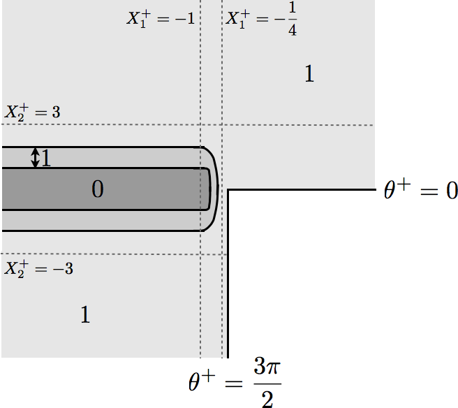
Figure 4: Schematic representation of the cut-off function $\chi_{\text{macro},+}$ defined in (4.7)

The functions $p_{m,q,+}$ are polynomials in $\ln|X_{1}^{+}|$. They are periodic with respect to $X_{1}^{+}$ and exponentially decaying as $X_{2}^{+}$ tends to $\pm\infty$. The functions $w_{m,q,+}$ are polynomials in $\ln R^{+}$. Note that, for $R^{+}$ large enough, if $X_{1}^{+}<-1$,

$$\mathcal{U}_{m,p,+}=\sum_{r=0}^{p}\Big{(}(R^{+})^{\lambda_{m}-r}w_{m,r,+}(\ln R^{+},\theta^{+})\chi(X_{2}^{+})+|X_{1}^{+}|^{\lambda_{{m}}-r}p_{m,r,+}(\ln|X_{1}^{+}|,X_{1}^{+},X_{2}^{+})\Big{)}\quad$$ (4.10)

and, if $X_{1}^{+}>-1$,

$$\mathcal{U}_{m,p,+}=\sum_{r=0}^{p}(R^{+})^{\lambda_{m}-r}w_{m,r,+}\ .$$ (4.11)

The usage of the cut-off functions $\chi_{\text{macro},+}$, $\chi_{-}(X_{1}^{+})$, and $\chi(R^{+})$ in (4.8) is simply a technical way to construct function defined on the whole domain $\widehat{\Omega}^{+}$ (and more precisely belonging to $H^{2}_{\text{loc}}(\widehat{\Omega}^{+})$) that coincides with $\mathcal{U}_{m,p,+}$ for large $R^{+}$ as given in (4.10) and (4.11).

Remark 4.4.

In view of Proposition 4.2, reminding that $p_{m,0}(\ln|X_{1}^{+}|,X_{1}^{+},X_{2}^{+})$ is proportional to $(1-\chi(X_{2}^{+}))$, for any $\gamma\in(1/2,1)$, the asymptotic block $\mathcal{U}_{m,p,+}$ belongs to $\mathfrak{V}_{\beta,\gamma}^{2}(\widehat{\Omega}^{+})$ for any $\beta<1-\lambda_{m}$.

Defining $\chi_{\text{macro},-}(X_{1}^{-},X_{2}^{-})=\chi_{\text{macro},+}(-X_{1}^{-},X_{2}^{-})$, we can also define the asymptotic blocks associated with $\widehat{\Omega}^{-}$ as follows:

$$\mathcal{U}_{m,p,-}=\chi(R^{-})\sum_{r=0}^{p}\Big{(}\chi_{\text{macro},-}(X_{1}^{-},X_{2}^{-})\,(R^{-})^{\lambda_{m}-r}\,w_{m,r,-}(\ln R^{-},\theta^{-})+\\[-8.00003pt] \chi_{+}(X_{1}^{-})\,|X_{1}^{-}|^{\lambda_{m}-r}p_{m,r,-}(\ln|X_{1}^{-}|,X_{1}^{-},X_{2}^{-})\Big{)}.$$ (4.12)

We are now in a position to write the main result of this subsection, which proves that for $R^{+}$ large and for sufficiently decaying right-hand sides, the solutions of Problem (4.1) can be decomposed into a sum of radial contributions corrected by periodic exponentially decaying correctors in the vicinity of the layer of equispaced holes. In the following, a real number $\beta$ is said to be admissible if $\beta-1\notin\Lambda$.

Proposition 4.5.

Let $k\in\mathbb{N}$ and $\gamma\in(1/2,1)$. Assume that $f\in\mathfrak{V}_{\beta,\gamma}^{0}(\widehat{\Omega}^{+})$ for some admissible $\beta>\max(3,1+\frac{2(k+1)}{3})$ (and so $\sqrt{1+(R^{+})^{2}}f\in L^{2}(\widehat{\Omega}^{+})$) and that $g\in H^{1/2}(\widehat{\Gamma}_{\text{\rm hole}})$ is compactly supported. Then, the unique solution $u$ of Problem (4.1) belongs to $\mathfrak{V}(\widehat{\Omega}^{+})\cap\mathfrak{V}_{\beta^{\prime},\gamma}^{2}(\widehat{\Omega}^{+})$ for any $\beta^{\prime}<\frac{1}{2}$. Moreover, $u$ admits, for $\gamma-1$ sufficiently small, the decomposition

$$u=\sum_{n=1}^{k}\mathscr{L}_{-n}(u)\,{\mathcal{U}_{-n,p(n),+}}+\;\tilde{u},\quad p(n)=\max(1,\lceil\frac{2}{3}(k-n)\rceil),$$ (4.13)

where the asymptotic blocks $\mathcal{U}_{-n,p(n),+}$ are defined in (4.8), $\mathscr{L}_{-n}(u)$, $1\leq n\leq k$, denote $k$ constants, and, the remainder $\tilde{u}\in\mathfrak{V}_{\beta^{0},\gamma}^{2}(\widehat{\Omega}^{+})$ for any $\beta^{0}$ such that $\beta^{0}<\beta$. In addition, there exists a constant $C>0$ such that

$$\|\tilde{u}\|_{\mathfrak{V}_{\beta^{0},\gamma}^{2}(\widehat{\Omega}^{+})}+\sum_{n=1}^{k}\left|\mathscr{L}_{-n}(u)\right|\quad\leq\quad C\left(\|f\|_{\mathfrak{V}_{\beta,\gamma}^{0}(\widehat{\Omega}^{+})}+\|g\|_{H^{1/2}(\widehat{\Gamma}_{\text{\rm hole}})}\right).$$ (4.14)

We remind that $\lceil a\rceil$ (used in (4.13)) stands for the smallest integer not less than $a$.

The proof of Proposition 4.5, postponed in Appendix D.3, deeply relies on successive applications of the following lemma, which is a direct adaptation of Theorem 4.1 in [32]. To long to be presented in this paper, its proof requires the use of involved tools of complex analysis that are fully described in [32].

Lemma 4.6.

Let $\gamma\in(\frac{1}{2},1)$. Let $\beta^{1}$ and $\beta^{2}$ be two admissible exponents such that $\beta^{1}<\beta^{2}$ and $\beta^{2}-\beta^{1}<1$. Assume that $u\in\mathfrak{V}_{\beta^{1},\gamma}^{2}(\widehat{\Omega}^{+})$ satisfies Problem (4.1) with $f\in\mathfrak{V}_{\beta^{2},\gamma}^{0}(\widehat{\Omega}^{+})$ and a compactly supported $g\in H^{1/2}(\widehat{\Gamma}_{\text{\rm hole}})$. Then, for $\gamma-1<0$ sufficiently small $u$ admits the decomposition

$$u=\sum_{\frac{3}{2}(1-\beta^{2})<k<\frac{3}{2}(1-\beta^{1})}c_{k}\,\mathcal{U}_{k,3,+}\,+\tilde{u},$$ (4.15)

where the asymptotic blocks $\mathcal{U}_{k,3,+}$ are defined in (4.8) and for any admissible $\beta^{0}\in(\beta^{1},\beta^{2})$ the remainder $\tilde{u}\in\mathfrak{V}_{\beta^{0},\gamma}^{2}(\widehat{\Omega}^{+})$. In this case, there exists a positive constant $C>0$ such that

$$\|\tilde{u}\|_{\mathfrak{V}_{\beta^{0},\gamma}^{2}(\widehat{\Omega}^{+})}+\sum_{\frac{3}{2}(1-\beta^{2})<k<\frac{3}{2}(1-\beta^{1})}|c_{k}|\quad\leq\quad C\left(\|{u}\|_{\mathfrak{V}_{\beta^{1},\gamma}^{2}(\widehat{\Omega}^{+})}+\|f\|_{\mathfrak{V}_{\beta^{2},\gamma}^{0}(\widehat{\Omega}^{+})}+\|g\|_{H^{1/2}(\widehat{\Gamma}_{\text{\rm hole}})}\right).$$ (4.16)

We emphasize that the powers of $R^{+}$ (or $X_{1}^{+}$) appearing in (4.13) (see (4.8)) are of the form $-\frac{2}{3}n-q$, $n\in\mathbb{N}^{\ast}$, $q\in\mathbb{N}$. Thus, they coincide with the ones obtained for the far field part (see for instance Proposition 3.8). Moreover, as can be expected, the ’leading’ singular exponents ${\frac{2n}{3}}$ correspond to those of the problem without periodic layer (here again, as for the macroscopic terms).

Remark 4.7.

The assumption on $g$ in Proposition 4.5 and Lemma 4.6 could be weakened by using the trace spaces associated with the weighted Sobolev spaces $\mathfrak{V}_{\beta,\gamma}^{\ell}(\widehat{\Omega}^{+})$ (see [32]).

4.2 Two families of near field singularities

This subsection is dedicated to the construction of two families of functions $S_{m}^{\pm}$, $m\in\mathbb{N}^{\ast}$, hereinafter referred to as the near field singularities for the right and left corner, satisfying the homogeneous Poisson problems

$$\left\{\begin{aligned} -\Delta S_{m}^{\pm}&\;=&0&\quad\mbox{in}\;\widehat{\Omega}^{\pm},\\ S_{m}^{\pm}&\;=&0&\quad\mbox{on}\;\partial\mathcal{K}^{\pm},\\ \partial_{n}S_{m}^{\pm}&\;=&0&\quad\mbox{on}\;\partial\widehat{\Omega}^{\pm}\setminus\partial\mathcal{K}^{\pm}\ ,\end{aligned}\right.$$ (4.17)

and behaving like $(R^{\pm})^{\lambda_{m}}w_{m,0,\pm}(\theta^{{{}^{\pm}}})$ for $R^{\pm}$ large, where $w_{m,0,+}=\sin(\frac{2n}{3}{\theta^{+}})$ and $w_{m,0,-}=\sin(\frac{2n}{3}(\theta^{-}-\frac{\pi}{2}))$ (defined in Proposition 3.2).

Proposition 4.8.

There exists a unique function $S_{m}^{+}\in\mathfrak{V}_{\beta,\gamma}^{2}(\widehat{\Omega}^{+})$ for any $\beta<1-\lambda_{m}$ and $\gamma\in(1/2,1)$, satisfying the homogeneous equation (4.17) such that the function

$$\tilde{S}_{m}^{+}=S_{m}^{+}-\mathcal{U}_{m,\lceil 1+\lambda_{m}\rceil,+}$$ (4.18)

belongs to $\mathfrak{V}(\widehat{\Omega}^{+})$. Moreover, for any $k\in\mathbb{N}^{\ast}$, choosing $1-\gamma$ sufficiently small, there exists a function $\mathcal{R}_{m,k}\in\mathfrak{V}_{\beta^{0},\gamma}^{2}(\widehat{\Omega}^{+})$ for any admissible $\beta^{0}<1+\frac{2(k+1)}{3}$ and $k$ constants $\mathscr{L}_{-n}(S_{m}^{+})$ ($1\leq k\leq n$) such that $S_{m}^{+}$ admits the decomposition

$$S_{m}^{+}=\mathcal{U}_{m,\lceil\frac{2(k+m)}{3}\rceil,+}+\sum_{n=1}^{k}\mathscr{L}_{-n}(S_{m}^{+})\mathcal{U}_{-n,\lceil\frac{2(k-n)}{3}\rceil,+}+\mathcal{R}_{m,k}.$$ (4.19)

In addition, for any $\beta<1-\lambda_{m}$, there is a constant $C>0$ such that

$$\sum_{n=1}^{k}\left|\mathscr{L}_{-n}(S_{m}^{+})\right|+\left\|\mathcal{R}_{m,k}\right\|_{\mathfrak{V}_{2,\beta^{0}}^{2}(\widehat{\Omega}^{+})}\leq C\,\left\|S_{m}^{+}\right\|_{\mathfrak{V}_{2,\beta}^{2}(\widehat{\Omega}^{+})}.$$ (4.20)

In the same way as the near field singularities for the right corner $S_{m}^{+}$, the near field singularities for the left corner $S_{m}^{-}$ can be defined. Note that for $m\geq 2$ there are several functions satisfying the homogeneous equations (4.17) and behaving like $(R^{+})^{\lambda_{m}}w_{m,0,+}$ (leading term) for large $R^{+}$. Indeed, admitting the existence of the functions $S_{m}^{+}$, any function of the form $S_{m}^{+}+\sum_{k=1}^{m-1}a_{k}S_{k}^{+}$ would also fulfill these requirements. Nevertheless, the (4.19) restores the uniqueness by fixing (arbitrary) $a_{k}$, $k=1,\ldots,m-1$ to $0$.

Proof.

The proof is classical and is very similar to the proof of Propositions 3.5, 3.6 and 3.8. We first prove the existence of $S_{m}^{+}$. The function $\tilde{S}_{m}^{+}$ satisfies

$$\left\{\begin{aligned} -\Delta\tilde{S}_{m}^{+}&\;=&\tilde{f}_{m}&\quad\mbox{in}\;\widehat{\Omega}^{+},\\ \tilde{S}_{m}^{+}&\;=&0&\quad\mbox{on}\;\partial\mathcal{K}^{+},\\ \partial_{n}\tilde{S}_{m}^{+}&\;=&0&\quad\mbox{on}\;\partial\widehat{\Omega}^{+}\setminus\partial\mathcal{K}^{+},\end{aligned}\right.\quad\tilde{f}_{m}=-\Delta\mathcal{U}_{m,\lceil 1+\lambda_{m}\rceil,+}.$$

In view of Lemma 4.3, $\tilde{f}_{m}$ belongs to $\mathfrak{V}_{2,\beta}^{0}(\widehat{\Omega}^{+})$ for $\beta<2-\lambda_{m}+\lceil 1+\lambda_{m}\rceil$. Noting that $2-\lambda_{m}+\lceil 1+\lambda_{m}\rceil{\geqslant}3$, Proposition 4.1 ensures the existence and uniqueness of $\tilde{S}_{m}^{+}\in\mathfrak{V}(\widehat{\Omega}^{+})$, and, hence, the existence of $S_{m}^{+}$. Uniqueness of $S_{m}^{+}$ follows directly from the fact that difference of two possible solutions is in the variational space $\mathfrak{V}(\widehat{\Omega}^{+})$ and satisfies (4.17). Finally, the asymptotic behavior for large $R^{+}$ results from a direct application of Proposition 4.5 to the function $\tilde{S}_{m}^{+}-\mathcal{U}_{m,p,+}$ choosing $p$ sufficiently large so that $\Delta(\tilde{S}_{m}^{+}-\mathcal{U}_{m,p,+})$ belongs to $\mathfrak{V}_{\beta,\gamma}^{2}(\widehat{\Omega}^{+})$ for a real number $\beta>\max(3,1+\frac{2(k+1)}{3})$ (which is, thanks to Lemma 4.3, always possible). ∎

4.3 An explicit expression for the near field terms

As done for the macroscopic terms in Section 3.4, we can write a quasi-explicit formula for the near field terms $U_{n,q,\pm}^{\delta}$. We shall impose that the functions $U_{n,q,\pm}^{\delta}$ do not blow up faster than $(R^{+})^{\lambda_{n}}$ for $R^{+}\to\infty$. Since $U_{n,q,\pm}^{\delta}$ satisfies the near field equations (1.18), it is natural to construct $U_{n,q,\pm}^{\delta}$ as a linear combination of the near field singularities $S_{k}^{\pm}$, $1\leq k\leq n$, namely

$$U_{n,q,\pm}^{\delta}=\sum_{k=1}^{n}\mathscr{L}_{k}(U_{n,q,\pm}^{\delta})S_{k}^{\pm},$$ (4.21)

where $\mathscr{L}_{k}(U_{n,q,\pm}^{\delta})$ are constants that will be determined by the matching procedure and that might depend on $\delta$. Naturally, the functions $U_{n,q,\pm}$ (defined by (4.21)) satisfy the near field equations (1.18) and belong to $\mathfrak{V}_{\beta,\gamma}^{2}(\widehat{\Omega}^{\pm})$ for any $\beta<1-\lambda_{n}$ and $\gamma\in(1/2,1)$. It is worth noting that the definition (4.21) implies that

$$U_{0,q,\pm}^{\delta}=0\quad\forall q\in\mathbb{N}.$$ (4.22)

Asymptotic behavior for large $R^{+}$

To conclude this section, we slightly anticipate the upcoming matching procedure by writing the behavior of $U_{n,q,+}^{\delta}$ at infinity. Thanks to the asymptotic behavior of $S_{m}^{+}$ for $R^{+}\to\infty$ (Proposition 4.8), we see that, for any $K\in\mathbb{N}^{\ast}$,

$$U_{n,q,+}^{\delta}=\sum_{k=1}^{n}\sum_{l=-k}^{K}\mathscr{L}_{k}(U_{n,q,+}^{\delta})\,\mathscr{L}_{-l}(S_{k}^{+})\,{\mathcal{U}_{-l,\lceil\frac{2(K-l)}{3}\rceil,+}}\;+\;\mathcal{R}_{n,q,K,+},$$ (4.23)

where $\mathcal{R}_{n,q,K,+}\in\mathfrak{V}_{2,\beta^{0}}^{2}(\widehat{\Omega}^{+})$ for any $\beta^{0}<1+\frac{2(K+1)}{3}$. Here, for the sake of concision, we have posed

$$\mathscr{L}_{r}(S_{q}^{+})=0\quad\mbox{for any }r\in\mathbb{N}\;\text{such that}\;0\leq r\leq q-1,$$

and $\mathcal{U}_{0,j,+}=0$ for any $j\in\mathbb{N}$. Then, substituting the asymptotic blocks $\mathcal{U}_{-l,k+2-l,+}$ for their explicit expression (4.8), we obtain the decomposition

$$\begin{aligned} U_{n,q,+}^{\delta}&=\chi_{\text{macro},+}(\mathbf{X})\sum_{l=-n}^{K}\sum_{r=0}^{{\lceil\frac{2(K-l)}{3}\rceil}}A_{n,q,-l,+}^{\delta}\left(R^{+}\right)^{-\frac{2l}{3}-r}w_{-l,r,+}(R^{+},\theta^{+})\\ &\hskip 10.00002pt+\chi_{-}(X_{1}^{+})\sum_{l=-n}^{K}\sum_{r=0}^{\lceil\frac{2(K-l)}{3}\rceil}A_{n,q,-l,+}^{\delta}|X_{1}^{+}|^{-\frac{2l}{3}-r}p_{-l,r,+}(\ln|X_{1}^{+}|,X_{1}^{+},X_{2}^{+})+\mathcal{R}_{n,q,K,+}\ ,\end{aligned}$$ (4.24)

where we have used the convention $w_{0,r,+}=0$ and $p_{0,r,+}=0$ for any $r\in\mathbb{Z}$. Here,

$$\forall(n,q,l)\in\mathbb{N}^{2}\times\mathbb{Z},\quad A_{n,q,l,+}^{\delta}=\sum_{k=\max(1,l)}^{n}\mathscr{L}_{k}(U_{n,q,+}^{\delta})\mathscr{L}_{l}(S_{k}^{+}).$$ (4.25)

Note that for $n=0$, $A_{n,q,l,+}^{\delta}=0$. Moreover, for $l\geq 0$, $\mathscr{L}_{l}(S_{k})=\delta_{l,k}$, and consequently

$$A_{n,q,l,+}^{\delta}=\mathscr{L}_{l}(U_{n,q,+}^{\delta}).$$ (4.26)

Finally, with the change of index $-l\to m$ and summing up over $n$ and $q$, we can formally obtain an asymptotic series of the near field: For $X_{1}^{+}<-1$,

$$\sum_{(n,q)\in\mathbb{N}^{2}}\delta^{\frac{2n}{3}+q}U_{n,q,+}^{\delta}=\\ \sum_{(n,q)\in\mathbb{N}^{2}}\delta^{\frac{2n}{3}+q}\sum_{m=-\infty}^{n}A_{n,q,m,+}^{\delta}\sum_{r\in\mathbb{N}}\left((R^{+})^{\frac{2m}{3}-r}w_{m,r,+}(\theta^{+},{\ln R^{+}})\chi(X_{2}^{+})\right.+\left.|X_{1}^{+}|^{\frac{2m}{3}-r}p_{m,r,+}(\ln|X_{1}^{+}|,\mathbf{X}^{+})\right)$$ (4.27)

and, for $X_{1}^{+}>-1$,

$$\sum_{(n,q)\in\mathbb{N}^{2}}\delta^{\frac{2n}{3}+q}U_{n,q,+}^{\delta}=\sum_{(n,q)\in\mathbb{N}^{2}}\delta^{\frac{2n}{3}+q}\sum_{m=-\infty}^{n}A_{n,q,m,+}^{\delta}\sum_{r\in\mathbb{N}}(R^{+})^{\frac{2m}{3}-r}w_{m,r,+}(\theta^{+},\ln R^{+})\ .$$ (4.28)

The near field terms $U_{n,q,-}^{\delta}$ can be decomposed in strictly similar way by substituting formally the superscript plus into a superscript minus in (4.24) and (4.25). Here, it should be noted that the way to compute $\mathscr{L}_{l}(U_{n,q,-}^{\delta})$ is different how $\mathscr{L}_{l}(U_{n,q,+}^{\delta})$ are computed.

5 Matching procedure and construction of the far and near field terms

We are now in the position to write the matching conditions that account for the asymptotic coincidence of the far field expansion with the near field expansion in the matching areas. Based on the matching conditions, we provide an iterative algorithm to define all the terms of the far and near field expansion (to any order), which have not been fixed yet.

5.1 Far field expansion expressed in the microscopic variables

We start with writing the formal expansion of the far field $\sum_{(n,q)\in\mathbb{N}^{2}}\delta^{\frac{2n}{3}+q}(u_{n,q}^{\delta}(\mathbf{x})\chi(x_{2}/\delta)+\Pi_{n,q}^{\delta}(x_{1},\frac{\mathbf{x}}{\delta}))$ (cf. (1.7)) in the matching area located in the vicinity of the right corner (i. e. for small $r^{+}$). Collecting (3.28) and (3.31), summing over the pair of indices $(n,q)\in\mathbb{N}^{2}$ and applying the change of scale $\mathbf{x}^{+}/\delta=(\mathbf{x}-\mathbf{x}_{O}^{+})/\delta\to\mathbf{X}^{+}$ and so $r^{+}/\delta\to R^{+}$ we formally obtain for $X_{1}<-1$,

$$\sum_{(n,q)\in\mathbb{N}}\delta^{\frac{2n}{3}+q}\left(u_{n,q}^{\delta}(\mathbf{x})\chi(\frac{x_{2}}{\delta})+\Pi_{n,q}^{\delta}(x_{1},\frac{\mathbf{x}}{\delta})\right)=\\[-8.00003pt] \sum_{(n,q)\in\mathbb{N}^{2}}\delta^{\frac{2}{3}n+q}\sum_{m=-\infty}^{n}a_{n-m,q,m,+}^{\delta}\sum_{r\in\mathbb{N}}\Big{(}(R^{+})^{\frac{2m}{3}-r}w_{m,r,+}(\theta^{+},\ln R^{+}+\ln\delta)\chi(X_{2}^{+})\\[-8.00003pt] +|X_{1}^{+}|^{\frac{2m}{3}-r}p_{m,r,+}(\ln|X_{1}^{+}|+\ln\delta,X_{1}^{+},X_{2}^{+})\Big{)}\ ,$$ (5.1)

and for $X_{1}>-1$

$$\sum_{(n,q)\in\mathbb{N}}\delta^{\frac{2n}{3}+q}u_{n,q}^{\delta}(\mathbf{x})=\sum_{(n,q)\in\mathbb{N}^{2}}\delta^{\frac{2}{3}n+q}\sum_{m=-\infty}^{n}a_{n-m,q,m,+}^{\delta}\sum_{r\in\mathbb{N}}(R^{+})^{\frac{2m}{3}-r}w_{m,r,+}(\theta^{+},\ln R^{+}+\ln\delta)\ .$$ (5.2)

Note, that the coefficients $a_{n,q,m,+}^{\delta}$, defined in (3.29), depend for $n>0$ on $\delta$ only through the constants $\ell^{\pm}_{-k}(u^{\delta}_{n,p})$, which we are going to fix in the matching process. In the equations (5.1) and (5.2) the terms $w_{m,r,+}$ and $p_{m,r,+}$ appear with a second shifted argument, i. e., $\ln R^{+}+\ln\delta$ instead of $\ln R^{+}$ and $\ln|X_{1}^{+}|+\ln\delta$ instead of $\ln|X_{1}^{+}|$. The following lemma is a reformulation of these terms as linear combinations of non-shifted ones and will prove very useful in the matching procedure. It is based essentially on the fact that the terms $w_{m,r,+}$ are polynomials in the second argument and $p_{m,r,+}$ in the first. The proof of the lemma finds itself in Appendix E.

Lemma 5.1.

The equalities

$$w_{m,r,\pm}(\theta^{{\pm}},\ln R^{{\pm}}+\ln\delta)=\sum_{k=0}^{\lfloor r/2\rfloor}w_{m-3k,r-2k,\pm}(\theta^{{\pm}},\ln R^{{\pm}})\;\sum_{i=0}^{k}C_{m,2k,i,\pm}\;(\ln\delta)^{i}\ ,$$ (5.3)

and

$$p_{m,r,\pm}(\ln|X_{1}^{{\pm}}|+\ln\delta,\mathbf{X}^{{\pm}})=\sum_{k=0}^{\lfloor r/2\rfloor}p_{m-3k,r-2k,\pm}(\ln|X_{1}^{{\pm}}|,\mathbf{X}^{{\pm}})\;\sum_{i=0}^{k}C_{m,2k,i,\pm}\;(\ln\delta)^{i}$$ (5.4)

hold true, where for any integer $i,k$ such that $0\leq i\leq k$ and using the notation $w_{m,2k,\pm}(\theta^{{\pm}},\ln R^{{\pm}})=\sum_{i=0}^{k}(\ln R^{{\pm}})^{i}w_{m,2k,i,\pm}(\theta^{+})$, the constants $C_{m,2k,i\pm}$ are given by

$$C_{m,2k,i,\pm}=\frac{4}{3\pi}\int_{I^{\pm}}w_{m,2k,i,\pm}(\theta^{{\pm}})w_{m-3k,0,\pm}(\theta^{{\pm}})d\theta^{{\pm}},\;\;I^{+}=(0,\frac{3\pi}{2}),\,I^{-}=(-\frac{\pi}{2},\pi).$$ (5.5)

Remark 5.2.

With the convention that $w_{0,0,\pm}=0$ it follows that $C_{m,2k,i,\pm}=0$ for $k=m/3$. Moreover, in view of the orthogonality conditions (C.15),(C.23), $C_{m,2k,0,\pm}$ always vanishes if $k\neq 0$ and $C_{m,0,0,\pm}=1$.

Inserting (5.3) into (5.2) and noting that $\frac{2}{3}(m-3k)-(r-2k)=\frac{2}{3}m-r$, we obtain

$$\sum_{(n,q)\in\mathbb{N}^{2}}\delta^{\frac{2n}{3}+q}u_{n,q}^{\delta}=\sum_{(n,q)\in\mathbb{N}^{2}}\delta^{\frac{2}{3}n+q}\sum_{m=-\infty}^{n}a_{n-m,q,m,+}^{\delta}\\ \sum_{r\in\mathbb{N}}\sum_{k=0}^{\lfloor r/2\rfloor}(R^{+})^{\frac{2(m-3k)}{3}-(r-2k)}w_{m-3k,r-2k,+}(\theta^{+},\ln R^{+})\sum_{i=0}^{k}C_{m,2k,i,+}(\ln\delta)^{i}.$$

Then, the changes of indices $r-2k\rightarrow r$ and $m-3k\rightarrow m$ give

$$\sum_{(n,q)\in\mathbb{N}^{2}}\delta^{\frac{2n}{3}+q}u_{n,q}^{\delta}=\sum_{(n,q)\in\mathbb{N}^{2}}\delta^{\frac{2}{3}n+q}\sum_{m=-\infty}^{n}\tilde{a}_{n-m,q,m,+}^{\delta}\sum_{r\in\mathbb{N}}(R^{+})^{\frac{2m}{3}-r}w_{m,r}(\theta^{+},\ln R^{+}),\quad{X_{1}^{+}>0},$$ (5.6)

where

$$\forall(n,q,l)\in\mathbb{N}^{2}\times\mathbb{Z},\quad\tilde{a}_{n,q,m,+}^{\delta}=\sum_{k=0}^{\lfloor n/3\rfloor}a_{n-3k,q,m+3k,+}^{\delta}\sum_{i=0}^{k}C_{m+3k,2k,i,+}(\ln\delta)^{i}\ .$$ (5.7)

In particular, for $m<0$, thanks to (3.30) (and using Remark 5.2), we have

$$\tilde{a}_{n,q,m,+}^{\delta}=\ell_{m}^{+}(u_{n,q}^{\delta})+\sum_{k=1}^{\lfloor n/3\rfloor}a_{n-3k,q,m+3k,+}^{\delta}\sum_{i=0}^{k}C_{m+3k,2k,i,+}(\ln\delta)^{i}.$$ (5.8)

Analogously, for $X_{1}^{+}<-1$, we obtain,

$$\sum_{(n,q)\in\mathbb{N}}\delta^{\frac{2n}{3}+q}(u_{n,q}^{\delta}(\mathbf{x})\chi(x_{2}{/\delta})+\Pi_{n,q}^{\delta}(x_{1},\mathbf{x}/\delta)=\\ \sum_{(n,q)\in\mathbb{N}^{2}}\delta^{\frac{2}{3}n+q}\sum_{m=-\infty}^{n}\tilde{a}_{n-m,q,m,+}^{\delta}\sum_{r\in\mathbb{N}}\left((R^{+})^{\frac{2m}{3}-r}w_{m,r,+}(\theta^{+},\ln R^{+})\chi(X_{2})\right.+\left.|X_{1}^{+}|^{\frac{2m}{3}-r}p_{m,r,+}(\ln|X_{1}^{+}|,\mathbf{X}^{+})\right).$$ (5.9)

The previous two expressions have to be compared with formula (4.27) and(4.28), in which the coefficients $A_{n,q,m,+}^{\delta}$ are still not determined, since the constants $\mathscr{L}_{m}(U_{n,q,+}^{\delta})$, $m=1,\ldots,n$ are not fixed yet. We aim to match the expansions in the matching zone and, hence, define these constants uniquely.

5.2 Derivation of the matching conditions

Arrived at this point, the derivation of the matching conditions is straight-forward. It suffices to identify formally all terms of the expansions (5.9) and (5.6) of the far field with all terms of the expansions (4.27) and  (4.28) for the near field. We end up with the following set of conditions:

$$A_{n,q,m,+}^{\delta}=\tilde{a}_{n-m,q,m,+}^{\delta},\quad\forall(n,q)\in\mathbb{N}^{2},\;\text{ and }\;m\in\mathbb{Z},\;m\leq n,$$ (5.10)

where $A_{n,q,m,+}^{\delta}$ and $\tilde{a}_{n-m,q,m,+}^{\delta}$ were defined in (4.25) and (5.7). As the coefficients $A_{n,q,m,+}^{\delta}$ are linear combinations of the constants $\mathscr{L}_{m}(U_{n,q,+}^{\delta})$, $m=1,\ldots,n$ and the coefficients $\tilde{a}_{n,q,m,+}^{\delta}$ are linear combinations of the constants $\ell^{+}_{-m}(u_{n,p}^{\delta})$, $m=1,\ldots,n$ for some $p\in{\mathbb{N}}$ we aim now to obtain conditions between those constants. Here, we will proceed separately for the the cases $m>0$, $m=0$ and $m<0$.

For $0<m\leq n$, using the equality (4.26), we have for any $(n,q)\in\mathbb{N}^{\ast}\times\mathbb{N}$,

$$\mathscr{L}_{m}(U_{n,q,+}^{\delta})=\tilde{a}_{n-m,q,m,+}^{\delta}\ .$$ (5.11)

For $m=0$, for any $(n,q)\in\mathbb{N}$, there is nothing to be matched. Indeed, both left and right-hand sides of (5.10) vanish ($\tilde{a}_{n,q,0,+}=0$ because $C_{3k,2k,i,+}=0$, see Remark 5.2).

For $m<0$, in view of (5.8) and substituting $A_{n,q,m,+}$ for its definition (4.25), we have for any $(n,q)\in\mathbb{N}^{2}$,

$$\ell_{m}^{+}(u_{n-m,q}^{\delta})=-\sum_{k=1}^{\lfloor(n-m)/3\rfloor}a_{n-m-3k,q,m+3k,+}^{\delta}\sum_{i=0}^{k}C_{m+3k,2k,i,+}(\ln\delta)^{i}+\sum_{k=1}^{n}\mathscr{L}_{k}(U_{n,q,+}^{\delta})\mathscr{L}_{m}(S_{k}^{+}),$$ (5.12)

which may also be red as follows: for any $(n,q,m)\in\mathbb{N}^{3}$ such that, $n\geq 1$, and $1\leq m\leq n$,

$$\ell_{-m}^{+}(u_{n,q}^{\delta})=-\sum_{k=1}^{\lfloor n/3\rfloor}a_{n-3k,q,-m+3k,+}^{\delta}\sum_{i=0}^{k}C_{-m+3k,2k,i,+}(\ln\delta)^{i}+\sum_{k=1}^{n-m}\mathscr{L}_{k}(U_{n-m,q,+}^{\delta})\mathscr{L}_{{-m}}(S_{k}^{+}).$$ (5.13)

Here again, we can write similar matching conditions for the matching area located close to the left corner. These conditions link the macroscopic terms $u_{n,q}^{\delta}$ to the near field terms $U_{n,q,-}^{\delta}$: for $1\leq m\leq n$ and for any $(n,q)\in\mathbb{N}^{\ast}\times\mathbb{N}$,

$$\mathscr{L}_{m}(U_{n,q,-}^{\delta})=\tilde{a}_{n-m,q,m,-}^{\delta},$$ (5.14)

and, for any $(n,q,m)\in\mathbb{N}^{3}$ such that, $n\geq 1$, and $1\leq m\leq n$,

$$\ell_{-m}^{-}(u_{n,q}^{\delta})=-\sum_{k=1}^{\lfloor n/3\rfloor}a_{n-3k,q,-m+3k,-}^{\delta}\sum_{i=0}^{k}C_{-m+3k,2k,i,-}(\ln\delta)^{i}+\sum_{k=1}^{n-m}\mathscr{L}_{k}(U_{n-m,q,-}^{\delta})\mathscr{L}_{{-m}}(S_{k}^{-}).$$ (5.15)

Here, $\tilde{a}_{n,q,m}$ are defined by

$$\forall\,(n,q,l)\in\mathbb{N}^{2}\times\mathbb{Z},\quad\tilde{a}_{n,q,m,-}^{\delta}=\sum_{k=0}^{\lfloor n/3\rfloor}a_{n-3k,q,m+3k,-}^{\delta}\sum_{i=0}^{k}C_{m+3k,2k,i,-}(\ln\delta)^{i}\ ,$$

with

$$\forall\,(j,m)\in\mathbb{N}\times\mathbb{Z},\;a_{0,j,m,-}^{\delta}=\ell_{m}^{-}(s_{0,j}),\;\mbox{and}\;a_{n,j,m,-}^{\delta}=\sum_{\pm}\sum_{k=\max(1,-m)}^{n}\sum_{p=0}^{j}\ell_{-k}^{\pm}(u_{n,p}^{\delta})\ell_{m}^{-}(s_{-k,j-p}^{\pm})\;\mbox{if }n>0.$$

5.3 Construction of the terms of the asymptotic expansions

The matching conditions then allow us to construct the far field terms $u_{n,q}^{\delta}$ and $\Pi_{n,q}^{\delta}$, and the near field terms $U_{n,q,\pm}^{\delta}$ by induction on $n$. The base case is obvious since we have seen that the macroscopic terms $u_{0,q}^{\delta}$ are entirely determined by Proposition (3.10), the boundary layer correctors $\Pi_{0,q}$ are defined by (2.30), and the near field terms $U_{0,q,\pm}^{\delta}=0$, $q\in{\mathbb{N}}$ by (4.22).

Then, assuming that $u_{m,q}^{\delta}$ and $U_{m,q,\pm}^{\delta}$ are constructed for any $m\leq n-1$, we will see that (5.11),(5.13) and (5.14),(5.15) permit to define both $u_{n,q}^{\delta}$ (and consequently $\Pi_{n,q}^{\delta}$) and $U_{n,q,\pm}^{\delta}$ for any $q\in\mathbb{N}$.

Far field terms

We remind that, for a given $q\in\mathbb{N}$, the complete definition of the macroscopic terms $u_{n,q}^{\delta}$ only requires the knowledge of the $\ell_{-m}^{\pm}(u_{n,q}^{\delta})$ for any integer $m$ between $1$ and $n$. In fact, the conditions (5.13) define exactly $\ell_{-m}^{+}(u_{n,q}^{\delta})$: in the right-hand side of (5.13), the quantities $\mathscr{L}_{-m}(S_{k}^{+})$ are known ($S_{k}^{+}$ is uniquely defined) and $\mathscr{L}_{k}(U_{n-m,q,+}^{\delta})$ are known since $U_{n-m,q,+}^{\delta}$ are already defined (induction hypothesis). In addition, since

$$a_{n-3k,q,-m+3k,+}^{\delta}=\begin{cases}\displaystyle\sum_{\pm}\sum_{r=\max(1,m-3k)}^{n-3k}\sum_{p=0}^{q}\ell_{-r}^{\pm}(u^{\delta}_{n-3k,p})\,\ell_{-m+3k}^{+}(s_{-r,q-p}^{\pm})&\mbox{if}\;n-3k\neq 0,\\ \displaystyle\ell_{-m+3k}^{+}(s_{0,q})&\mbox{if}\;n-3k=0,\end{cases}$$

the coefficient $a_{n-3k,q,-m+3k,+}^{\delta}$ is well defined for any $k$ such that $1\leq k\leq\lfloor n/3\rfloor$ ($\ell_{-j}^{+}(u_{n-3k,q})$ is known by the induction hypothesis). Naturally the conditions (5.15) define $\ell_{-m}^{-}(u_{n,q}^{\delta})$ is the same way. Finally, the definition of the boundary layer terms $\Pi_{n,q}^{\delta}$ follows from (2.30).

Near field terms

Similarly, the definition of the near field terms $U_{n,q,\pm}^{\delta}$ requires the specification of the quantities $\mathscr{L}_{m}(U_{n,q,\pm}^{\delta})$ for any integer $m$ between $1$ and $n$. The condition (5.11) exactly provides this missing information for $U_{n,q,+}^{\delta}$. Indeed, in the right-hand side of (5.11), the computation of $\tilde{a}_{n-m,q,m,+}^{\delta}$ requires the knowledge of

$$a_{n-m-3k,q,m+3k,+}^{\delta}=\begin{cases}\displaystyle\sum_{\pm}\sum_{r=0}^{n-m-3k}\sum_{p=0}^{q}\ell_{-r}^{\pm}(u_{n-m-3k,p}^{\delta})\,\ell_{m+3k}^{+}(s_{-r,q-p}^{\pm})&\mbox{if}\;n-m-3k\neq 0,\\ \displaystyle\ell_{m+3k}^{+}(s_{0,q})&\mbox{if}\;n-m-3k=0.\end{cases}$$

for $k$ between $0$ and $\lfloor(n-m)/3\rfloor$. But, since $m>0$, $\ell_{-r}^{+}(u_{n-m-3k,p}^{\delta})$ are well defined thanks to the induction hypothesis. Then, $U_{n,q,+}^{\delta}$ is entirely determined. In the same way, the condition (5.14) allows us to define $U_{n,q,-}^{\delta}$ as well, replacing all occurences of $\ell^{+}_{m}(s^{\pm}_{-r,q-p})$ by $\ell^{-}_{m}(s^{\pm}_{-r,q-p})$, $m\in{\mathbb{Z}}$ and all occurences $\ell^{+}_{m}(s_{0,q})$ by $\ell^{-}_{m}(s_{0,q})$, $m\in{\mathbb{Z}}$ in the previous formulas.

Remark 5.3.

We point out that the variables $n$ and $q$ play a very different roles in the recursive construction of the terms of the asymptotic expansion. Indeed, the construction is by induction only in $n$. At the step $n$, we construct $u_{n,q}^{\delta}$, $\Pi_{n,q}^{\delta}$ and $U_{n,q,\pm}^{\delta}$ for any $q\in\mathbb{N}$.

6 Justification of the asymptotic expansion

To finish this paper, we shall prove the convergence of the asymptotic expansion. Our main result deals with the convergence of the truncated macroscopic series in a domain that excludes the two corners and the periodic thin layer:

Theorem 6.1.

Let $N_{0}>0$ such that $3N_{0}$ is an integer and let $D_{N_{0}}$ denote the set of couples $(n,q)\in\mathbb{N}^{2}$ such that $\frac{2}{3}n+q\leq N_{0}$. Furthermore, for a given number $\alpha>0$, let

$$\Omega_{\alpha}=\Omega^{\delta}\setminus(-L-\alpha,L+\alpha)\times(-\alpha,\alpha).$$

Then, there exist a constant $\delta_{0}>0$, a constant $C=C(\alpha,\delta_{0})>0$, and a constant $k=k(N_{0})\geq 0$ such that for any $\delta\in(0,\delta_{0})$

$$\|u^{\delta}-\sum_{(n,q)\in D_{N_{0}}}\delta^{\frac{2}{3}n+q}u_{n,q}^{\delta}\|_{H^{1}(\Omega_{\alpha})}\leq\;C\,\delta^{N_{0}+\frac{1}{3}}(\ln\delta)^{k}.$$ (6.1)

Remark 6.2.

With more sophisticated techniques than applied in this article it is possible to prove that the power of $\ln\delta$ in the previous theorem is $k=k(N_{0})=\lfloor\frac{1}{2}(N_{0}+\frac{1}{3})\rfloor$. The first logarithmic term appears for $N_{0}=\frac{5}{3}$.

6.1 The overall procedure

As usual for this kind of work (See e. g. [24] (Sect. 3), [21] (Sect. 5.1), [18] (Sect. 4)), the proof of the previous result is based on the construction of an approximation $u_{N_{0}}^{\delta}$ of the solution $u^{\delta}$ on the whole domain $\Omega^{\delta}$ obtained from the four truncated series (at order $N_{0}$) of the macroscopic terms, the boundary layer terms and the near field terms:

1. The truncated macroscopic series $u_{\text{macro},N_{0}}^{\delta}$: we introduce the macroscopic cut-off function

   $$\chi_{\text{macro},\text{total}}^{\delta}({\mathbf{x}})=\chi_{+}\left(\frac{x_{1}-L}{\delta}\right)\chi_{-}\left(\frac{x_{1}+L}{\delta}\right)\chi\left(\frac{x_{2}}{\delta}\right)\\ +\sum_{\pm}\chi_{\text{macro},\pm}\left(\frac{x_{1}\mp L}{\delta},\frac{x_{2}}{\delta}\right)\left(1-\chi_{\mp}\left(\frac{x_{1}\mp L}{\delta}\right)\right),$$ (6.2)

   which is equal to $1$ for $|x_{1}|>L$, and which coincides with $\chi(\frac{x_{2}}{\delta})$ in the region $|x_{1}|<L-\delta$ (see Fig. 5). The cut-off functions $\chi$, $\chi_{\pm}$ and $\chi_{\text{macro},\pm}$ are defined in (1.8)-(1.17) and (4.7). We then define the macroscopic approximation as follows:

   $$u_{\text{macro},N_{0}}^{\delta}=\chi_{\text{macro},\text{total}}^{\delta}({\mathbf{x}})\sum_{(n,q)\in D_{0}}\delta^{\frac{2}{3}n+q}u_{n,q}^{\delta}(\mathbf{x}).$$ (6.3)

2. The truncated periodic corrector series $\Pi_{N_{0}}^{\delta}$: it is given by

   $$\Pi_{N_{0}}^{\delta}(\mathbf{x})=(1-\chi(x_{2}))\chi_{+}(\frac{x_{1}-L}{\delta})\chi_{-}(\frac{x_{1}+L}{\delta})\sum_{(n,q)\in D_{0}}\delta^{\frac{2}{3}n+q}\Pi_{n,q}^{\delta}(x_{1},\frac{\mathbf{x}}{\delta}).$$ (6.4)

   The function $\chi_{+}(\frac{x_{1}-L}{\delta})\chi_{-}(\frac{x_{1}+L}{\delta})$ permits us to localize the function $\Pi_{N_{0}}^{\delta}(\mathbf{x})$ in the domain $|x_{1}|<L$ while the introduction of the function $(1-\chi(x_{2}))$ ensures that $\Pi_{N_{0}}^{\delta}(\mathbf{x})$ vanishes on $\Gamma_{D}$.

3. The truncated near field series $U_{N_{0},\pm}^{\delta}(\mathbf{x})$:

   $$U_{N_{0},\pm}^{\delta}(\mathbf{x})=\sum_{(n,q)\in D_{0}}\delta^{\frac{2}{3}n+q}U_{n,q}^{\delta}(\frac{\mathbf{x}}{\delta}).$$ (6.5)

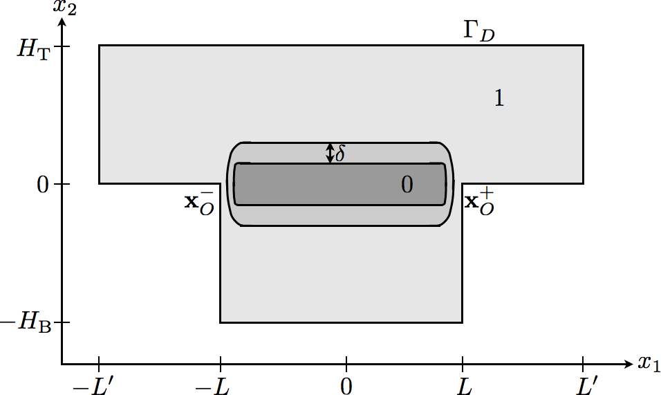
Figure 5: Schematic representation of the cut-off function $\chi_{\text{macro},\text{total}}^{\delta}$.

We shall construct a global approximation $u_{N_{0}}^{\delta}$ that coincides with $U_{N_{0},\pm}^{\delta}$ in the vicinity of the two corners, with $\Pi_{N_{0}}^{\delta}$ in the vicinity of the periodic layer and with $u_{\text{macro},N_{0}}^{\delta}$ away from the corners and the periodic layer. To do so, we introduce the cut off functions

$$\chi_{+}^{\delta}(\mathbf{x})=\chi\left(\frac{r^{+}}{\eta(\delta)}\right)\quad\mbox{and}\quad\chi_{-}^{\delta}(\mathbf{x})=\chi\left(\frac{r^{-}}{\eta(\delta)}\right),$$ (6.6)

where $\eta(\delta):\mathbb{R}^{+}\rightarrow\mathbb{R}^{+}$ is a smooth function such that

$$\lim_{\delta\rightarrow 0}\eta(\delta)=0\;\mbox{and}\;\lim_{\delta\rightarrow 0}\frac{\eta(\delta)}{\delta}=+\infty.$$ (6.7)

For instance for $s\in(0,1)$, $\eta(\delta)=\delta^{s}$ satisfies these conditions. Finally the global approximation $u_{N_{0}}^{\delta}$ of $u^{\delta}$ is defined by

$$u_{N_{0}}^{\delta}(\mathbf{x})=\chi_{+}^{\delta}(\mathbf{x})\,U_{N_{0},+}\;+\;\chi_{-}^{\delta}(\mathbf{x})\,U_{N_{0},-}\;+\;(1-\chi_{+}^{\delta}(\mathbf{x})-\chi_{-}^{\delta}(\mathbf{x}))\,(u_{\text{macro},N_{0}}^{\delta}(x)+\Pi_{N_{0}}^{\delta}(x)).$$ (6.8)

Note that $u_{N_{0}}^{\delta}$ belongs to $H^{1}_{\Gamma_{D}}(\Omega^{\delta})$ but does not satisfy homogeneous Neumann boundary conditions on $\Gamma^{\delta}$.

The aim of this part is to estimate the $H^{1}$-norm of the error $e_{N_{0}}^{\delta}=u^{\delta}-u_{N_{0}}^{\delta}$ in $\Omega^{\delta}$ (We remind that $u^{\delta}\in\mathrm{H}^{1}_{\Gamma_{D}}(\Omega^{\delta})$ is the ’exact’ solution, i. e. the solution of Problem (1.3)). It is in fact sufficient to estimate the residue $\Delta e_{N_{0}}^{\delta}$ and the Neumann trace $\partial_{n}e_{N_{0}}^{\delta}$. Then, the estimation of $\|e_{N_{0}}^{\delta}\|_{H^{1}(\Omega^{\delta})}$ directly results from a straightforward modification of the uniform stability estimate (1.5) (Proposition 1.1): there exists a constant $C>0$ such that, for $\delta$ small enough,

$$\|e_{N_{0}}^{\delta}\|_{H^{1}(\Omega^{\delta})}\leq C\left(\|\Delta e_{N_{0}}^{\delta}\|_{L^{2}(\Omega^{\delta})}+\|\partial_{n}e_{N_{0}}^{\delta}\|_{L^{2}(\Gamma^{\delta})}\right).$$ (6.9)

The main work of this part consists in proving the following proposition:

Proposition 6.3.

There exist a constant $C>0$ and a constant $\delta_{0}>0$ such that, for any $\varepsilon>0$, for any $\delta\in(0,\delta_{0})$,

$$\|\Delta e_{N_{0}}^{\delta}\|_{L^{2}(\Omega^{\delta})}+\|\partial_{n}e_{N_{0}}^{\delta}\|_{L^{2}(\Gamma^{\delta})}\leq C\left(\delta^{-2-\varepsilon}\left(\frac{\delta}{\eta(\delta)}\right)^{N_{0}}+\delta^{-1}\eta(\delta)^{N_{0}-\frac{1}{6}-\varepsilon}\right).$$ (6.10)

As a direct corollary, choosing $\eta(\delta)=\sqrt{\delta}$, $\varepsilon=\frac{1}{2}$, we obtain the following global error estimate: there exist a constant $C>0$ and a constant $\delta_{0}>0$ such that, for any $\delta\in(0,\delta_{0})$,

$$\|e_{N_{0}}^{\delta}\|_{H^{1}(\Omega^{\delta})}\leq\;C\,\delta^{\frac{N_{0}}{2}-\frac{5}{2}}.$$ (6.11)

Since $e_{N_{0}}^{\delta}$ coincides with $u^{\delta}-\sum_{(n,q)\in D_{N_{0}}}\delta^{\frac{2}{3}n+q}u_{n,q}^{\delta}$ in $\Omega_{\alpha}$ for $\delta$ small enough, Theorem 6.1 follows from (6.11) and the triangular inequality.

The remainder of this section is dedicated to the proof of Proposition 6.3. Although long and technical, the proof is rather standard.

Remark 6.4.

We emphasize that $u_{N_{0}}^{\delta}$ is certainly not the best choice to minimize the global error. As shown in [16], a global estimate based on the truncated far and near field terms obtained by the compound method might provide a better global error. Nevertheless, for the sake of simplicity and since we are mainly interested in the macroscopic error estimate (that can always be made optimal thanks to the triangular inequality), we prefer using here $u_{N_{0}}^{\delta}$.

6.2 Decomposition of the residue into a modeling error and a matching error

Remarking that the supports of the derivatives of $\chi_{+}^{\delta}$ and $\chi_{-}^{\delta}$ are disjoint (for $\delta$ small enough), using additionaly that $\Delta U_{N_{0},\pm}^{\pm}=0$, we can see that

$$-\Delta e_{N_{0}}^{\delta}=\mathcal{E}_{\text{mod}}+\mathcal{E}_{\text{match}},$$ (6.12)

where,

$$\mathcal{E}_{\text{match}}=-\sum_{\pm}[\Delta,\chi_{\pm}^{\delta}(\mathbf{x})](U_{N_{0},\pm}-u_{\text{macro},N_{0}}^{\delta}(x)-\Pi_{N_{0}}^{\delta}(x)),$$ (6.13)

and

$$\mathcal{E}_{\text{mod}}=f-(1-\chi_{+}^{\delta}(\mathbf{x})-\chi_{-}^{\delta}(\mathbf{x}))\Delta\left(u_{\text{macro},N_{0}}^{\delta}(x)+\Pi_{N_{0}}^{\delta}(x)\right).$$ (6.14)

Here, $\mathcal{E}_{\text{match}}$ represents the matching error. Its support, which coincides with the union of the supports of $\nabla\chi_{+}^{\delta}$ and $\nabla\chi_{-}^{\delta}$, is included in the union of the rings $\eta(\delta)<|r^{\pm}|<2\eta(\delta)$. It measures the mismatch between the far and near field truncated expansions in the matching zones. $\mathcal{E}_{\text{mod}}$, representing the modeling error (or consistency error), measures how the expansion fails to satisfies the original Laplace problem.

Similarly, is it easily seen that

$$\partial_{n}e_{N_{0}}^{\delta}=\sum_{\pm}\partial_{n}\chi_{\pm}^{\delta}(\mathbf{x})\left(U_{N_{0},\pm}-\Pi_{N_{0}}^{\delta}(x)\right),$$ (6.15)

so that the error on the boundary data in supported in the matching areas. Therefore its treatment will be similar to the one of the matching error.

In the next two sections, we shall estimate in turn $\mathcal{E}_{\text{mod}}$ (Section 6.3, Proposition 6.5) and $\mathcal{E}_{\text{match}}$ (Section 6.4 Proposition 6.8). The proof of Proposition 6.3 results from (6.12)-(6.15) and a direct application of these two propositions.

6.3 Estimation of the modeling error

The present section is dedicated to the proof of the following error estimate:

Proposition 6.5.

There exist a positive constant $\mathcal{C}_{\text{mod}}>0$ and a positive number $\delta_{0}>0$, such that, for any $\delta\in(0,\delta_{0})$,

$$\|\mathcal{E}_{\text{mod}}\|_{L^{2}(\Omega^{\delta})}\;\leq\;\mathcal{C}_{\text{mod}}\left(\frac{\delta}{\eta(\delta)}\right)^{N_{0}}\,\delta^{-\varepsilon-2}.$$ (6.16)

We first note that the intersection of the supports of $\nabla\chi_{\text{macro},\text{total}}^{\delta}({\mathbf{x}})$ (and $\Delta\chi_{\text{macro},\text{total}}^{\delta}({\mathbf{x}})$) and $1-\chi_{+}^{\delta}(\mathbf{x})-\chi_{-}^{\delta}(\mathbf{x})$ is included in the set

$$\Omega_{\text{mod}}^{\delta}=\{(x_{1},x_{2})\in\Omega^{\delta},|x_{1}|\leq L-\sqrt{\eta(\delta)-4\delta^{2}}\}.$$

Moreover, $\chi_{\text{macro},\text{total}}^{\delta}({\mathbf{x}})=\chi(\frac{x_{2}}{\delta})$ on this set. As a result,

$$f-(1-\chi_{+}^{\delta}(\mathbf{x})-\chi_{-}^{\delta}(\mathbf{x}))\Delta u_{\text{macro},N_{0}}^{\delta}(x)=-(1-\chi_{+}^{\delta}(\mathbf{x})-\chi_{-}^{\delta}(\mathbf{x}))1_{\Omega_{\text{mod}}^{\delta}}[\Delta,\chi(\frac{x_{2}}{\delta})]\left(\sum_{(n,q)\in D_{N_{0}}}\delta^{\frac{2}{3}n+q}u_{n,q}^{\delta}(\mathbf{x})\right),$$ (6.17)

where $1_{\Omega_{\text{mod}}^{\delta}}$ denotes the indicator function of $\Omega_{\text{mod}}^{\delta}$. In the previous formula, we used the macroscopic equations (1.13) (the functions $u_{n,q}^{\delta}$ are harmonic in $\Omega_{\mathrm{T}}\cup\Omega_{\mathrm{B}}$ unless for $n=q=0$ where $-\Delta u_{0,0}=0$). On the other hand,

$$-(1-\chi_{+}^{\delta}(\mathbf{x})-\chi_{-}^{\delta}(\mathbf{x}))\Delta\Pi_{N_{0}}^{\delta}(x)=-(1-\chi_{+}^{\delta}(\mathbf{x})-\chi_{-}^{\delta}(\mathbf{x}))1_{\Omega_{\text{mod}}^{\delta}}\sum_{(n,q)\in D_{N_{0}}}\delta^{\frac{2}{3}n+q}\Delta\Pi_{n,q}^{\delta}+\mathcal{E}_{\text{mod},1}$$ (6.18)

where,

$$\mathcal{E}_{\text{mod},1}=-(1-\chi_{+}^{\delta}(\mathbf{x})-\chi_{-}^{\delta}(\mathbf{x}))\,\left(\chi_{+}(\frac{x_{1}-L}{\delta})\chi_{-}(\frac{x_{1}+L}{\delta})(1-\chi(x_{2}))-1_{\Omega_{\text{mod}}^{\delta}}\right)\sum_{(n,q)\in D_{N_{0}}}\delta^{\frac{2}{3}n+q}\Delta\Pi_{n,q}^{\delta}\\ +(1-\chi_{+}^{\delta}(\mathbf{x})-\chi_{-}^{\delta}(\mathbf{x}))[\Delta,\chi_{+}(\frac{x_{1}-L}{\delta})\chi_{-}(\frac{x_{1}+L}{\delta})(1-\chi(x_{2}))]\sum_{(n,q)\in D_{N_{0}}}\delta^{\frac{2}{3}n+q}\Pi_{n,q}^{\delta}.$$ (6.19)

Collecting (6.17) and (6.18), we end up with

$$\mathcal{E}_{\text{mod}}=\mathcal{E}_{\text{mod},1}+\mathcal{E}_{\text{mod},2},$$ (6.20)

with

$$\mathcal{E}_{\text{mod},2}=-(1-\chi_{+}^{\delta}(\mathbf{x})-\chi_{-}^{\delta}(\mathbf{x}))1_{\Omega_{\text{mod}}^{\delta}}\sum_{(n,q)\in D_{N_{0}}}\delta^{\frac{2}{3}n+q}\left(\Delta\Pi_{n,q}^{\delta}(x_{1},\frac{\mathbf{x}}{\delta})+[\Delta,\chi(\frac{x_{2}}{\delta})]u_{n,q}^{\delta}(\mathbf{x})\right).$$ (6.21)

$\mathcal{E}_{\text{mod},1}$ is supported in a domain where $|x_{2}|>C\eta(\delta)$ wherein the periodic correctors $\Pi_{n,q}^{\delta}$ are exponentially decaying. As a result, $\mathcal{E}_{\text{mod},1}$ converges super-algebraically fast to $0$. More precisely, we can prove the following lemma, whose proof is left to the reader:

Lemma 6.6.

For any $N\in\mathbb{N}$, there exists a positive constant $C_{N}>0$ and a positive number $\delta_{0}>0$, such that, for any $\delta<\delta_{0}$,

$$\left\|\mathcal{E}_{\text{mod},1}\right\|_{L^{2}(\Omega^{\delta})}\leq C_{N}\delta^{N}.$$ (6.22)

It remains to estimate $\mathcal{E}_{\text{mod},2}$. Analogously to the case of an infinite thin periodic layer, we naturally use the periodic correctors equations (1.15). Nevertheless, the estimation requires a careful analysis because the fields $\Pi_{n,q}^{\delta}$ and $u_{n,q}^{\delta}$ are singular. We prove the following lemma, whose proof is postponed in Appendix F.1:

Lemma 6.7.

For any $\varepsilon>0$ sufficiently small, there exists a positive constant $C>0$ and a positive number $\delta_{0}>0$, such that, for any $\delta<\delta_{0}$,

$$\|\mathcal{E}_{\text{mod},2}\|_{L^{2}(\Omega^{\delta})}\leq C\left(\frac{\delta}{\eta(\delta)}\right)^{N_{0}}\,\delta^{-\varepsilon-2}.$$ (6.23)

Obviously, Proposition 6.5 is a straightforward consequence of (6.20), Lemma 6.6, and Lemma 6.7.

6.4 Estimation of the matching error

We now turn to the estimation of the matching error:

Proposition 6.8.

There exist a positive constant $\mathcal{C}_{\text{match}}>0$ and a positive number $\delta_{0}>0$, such that, for any $\delta<\delta_{0}$,

$$\|\mathcal{E}_{\text{match}}\|_{L^{2}(\Omega^{\delta})}\leq\mathcal{C}_{\text{match}}\left(\eta(\delta)^{-1}\,\left(\frac{\delta}{\eta(\delta)}\right)^{N_{0}-1-\varepsilon}+\delta^{-1}\eta(\delta)^{N_{0}+\frac{1}{3}-\varepsilon}\right),$$ (6.24)

and

$$\|\partial_{n}e_{N_{0}}^{\delta}\|_{L^{2}(\Gamma^{\delta})}\leq\mathcal{C}_{\text{match}}\left(\eta(\delta)^{-\frac{1}{2}}\,\left(\frac{\delta}{\eta(\delta)}\right)^{N_{0}-\varepsilon-5/3}+\delta^{-\frac{1}{2}}\eta(\delta)^{N_{0}-\frac{2}{3}-\varepsilon}\right).$$ (6.25)

We shall evaluate $\|\mathcal{E}_{\text{match}}\|_{L^{2}(\Omega^{\delta})}$ and $\|\partial_{n}e_{N_{0}}^{\delta}\|_{L^{2}(\Gamma^{\delta})}$ in turn. Both of these functions are supported in the overlapping areas. The function $\mathcal{E}_{\text{match}}$ is supported in the overlapping areas $\Omega_{\text{match}}^{\pm}$

$$\Omega_{\text{match}}^{\pm}=\left\{(x_{1},x_{2})\in\Omega^{\delta},\eta(\delta)\leq r^{\pm}\leq 2\eta(\delta)\right\}.$$

and $\|\partial_{n}e_{N_{0}}^{\delta}\|_{L^{2}(\Gamma^{\delta})}$ is supported in

$$\Gamma_{\text{match}}^{\pm}=\left\{(x_{1},x_{2})\in\Gamma^{\delta},\eta(\delta)\leq r^{\pm}\leq 2\eta(\delta)\right\}.$$

We shall estimate $\|\mathcal{E}_{\text{match}}\|_{L^{2}(\Omega_{\text{match}}^{+})}$ (resp. $\|\partial_{n}e_{N_{0}}^{\delta}\|_{L^{2}(\Gamma_{\text{match}}^{+})}$) but a similar analysis can be made for $\|\mathcal{E}_{\text{match}}\|_{L^{2}(\Omega_{\text{match}}^{-})}$ (resp. $\|\partial_{n}e_{N_{0}}^{\delta}\|_{L^{2}(\Gamma_{\text{match}}^{-})}$)).

We start with the computation of $U_{N_{0},+}^{\delta}-u_{\text{macro},N_{0}}^{\delta}(x)-\Pi_{N_{0}}^{\delta}$, which, thanks to the matching conditions (5.10), is expected to be small. The following computation is based on an expansion of the truncated series of far and near field terms in the overlapping area.

6.4.1 Expansion of $u_{\text{macro},N_{0}}^{\delta}$, $\Pi_{BL,N_{0}}^{\delta}$ and $U_{N_{0},+}^{\delta}$ in the overlapping area $\Omega_{\text{match}}^{+}$

For any couple $(n,q)\in\mathbb{N}^{2}$, we consider the integer $k(n,q,N_{0})$ given by

$$k(n,q,N_{0})=\left\{\begin{array}[]{ll}\frac{3}{2}(N_{0}-q)-n&\mbox{if $N_{0}$ and $q$ have the same parity},\\[4.30554pt] \frac{3}{2}(N_{0}-q)-n-\frac{1}{2}&\mbox{otherwise}.\end{array}\right.$$

Macroscopic truncated series $u_{\text{macro},N_{0}}^{\delta}$.

In view of (3.28), for any $(n,q)\in D_{N_{0}}$, there exists a function $\mathcal{R}_{\text{macro},n,q,\delta}\in V_{2,\beta}^{2}(\Omega_{\mathrm{T}})\cap V_{2,\beta}^{2}(\Omega_{\mathrm{B}})$ for any $\beta>1-\frac{2(k(n,q,N_{0})+1)}{3}$

$$u_{n,q}^{\delta}=\tilde{u}_{n,q}^{\delta}+\mathcal{R}_{\text{macro},n,q,\delta}\quad\quad\tilde{u}_{n,q}^{\delta}=\sum_{r=0}^{q}\sum_{m=-n}^{\frac{3}{2}(N_{0}+r-q)-n}a_{n,q-r,m,+}^{\delta}(r^{+})^{\frac{2m}{3}-r}w_{m,r,+}(\theta^{+},\ln r^{+}).$$ (6.26)

The reader may verify that, for non negative integer $r$, $k(n,q,N_{0})+\lfloor\frac{3r}{2}\rfloor\leq\lfloor\frac{3}{2}(N_{0}+r-q)-n\rfloor$. Then, a direct computation shows that

$$\sum_{(n,q)\in D_{N_{0}}}\delta^{\frac{2n}{3}+q}\tilde{u}_{n,q}^{\delta}(R^{+}\delta,\theta^{+})=\\ \sum_{(n,q)\in D_{N_{0}}}\delta^{\frac{2}{3}n+q}\sum_{m=-\alpha_{n,q}}^{n}\sum_{r=0}^{\frac{2}{3}(\alpha_{n,q}+m)}a_{n,q,m-n,+}^{\delta}(R^{+})^{\frac{2m}{3}-r}w_{m,r,+}(\theta^{+},\ln(R^{+}\delta)),$$

where $\alpha_{n,q}=\frac{3}{2}(N_{0}-q)-n$. Then, using Lemma 5.1, reproducing the calculations of (5.6) and using the matching conditions (5.10), we see that

$$\sum_{(n,q)\in D_{N_{0}}}\delta^{\frac{2n}{3}+q}\tilde{u}_{n,q}^{\delta}(R^{+}\delta,\theta^{+})=\sum_{(n,q)\in D_{N_{0}}}\delta^{\frac{2}{3}n+q}\sum_{m=-\alpha_{n,q}}^{n}{A}_{n,q,m,+}^{\delta}\sum_{r=0}^{\frac{2}{3}(\alpha_{n,q}+m)}(R^{+})^{\frac{2}{3}m-r}w_{m,r,+}(\theta^{+},\ln R^{+}).$$ (6.27)

Finally, noticing that $\chi_{\text{macro},\text{total}}^{\delta}(x)=\chi_{\text{macro},+}^{\delta}\left(\frac{x_{1}-L}{\delta},\frac{x_{2}}{\delta}\right)$ in $\Omega_{\text{match}}^{+}$, the truncated macroscopic series $u_{\text{macro},N_{0}}^{\delta}$ can be written as

$$u_{\text{macro},N_{0}}^{\delta}(\mathbf{x})=\chi_{\text{macro},+}(\mathbf{X}^{+})\left(\sum_{(n,q)\in D_{N_{0}}}\delta^{\frac{2}{3}n+q}\sum_{m=-\alpha_{n,q}}^{n}{A}_{n,q,m,+}^{\delta}\sum_{r=0}^{\frac{2}{3}(\alpha_{n,q}+m)}(R^{+})^{\frac{2}{3}m-r}w_{m,r,+}(\theta^{+},\ln R^{+})\right)\\ +\mathcal{R}_{\text{macro},N_{0}}^{\delta}(\mathbf{x})$$ (6.28)

where

$$\mathcal{R}_{\text{macro},N_{0}}^{\delta}(\mathbf{x})=\chi_{\text{macro},+}(\mathbf{X}^{+})\sum_{(n,q)\in D_{N_{0}}}\delta^{\frac{2}{3}n+q}\mathcal{R}_{\text{macro},n,q,\delta}(\mathbf{x}).$$ (6.29)

Boundary layer correctors series $\Pi_{BL,N_{0}}^{\delta}$.

Similarly, the asymptotic formula (3.31) for the periodic corrector $\Pi_{n,q}^{\delta}$ associated with the matching conditions (5.10) gives

$$\Pi_{BL,N_{0}}^{\delta}(\mathbf{x})=\chi_{-}(\mathbf{X}^{+})\left(\sum_{(n,q)\in D_{N_{0}}}\delta^{\frac{2}{3}n+q}\sum_{m=-\alpha_{n,q}}^{n}{A}_{n,q,m,+}^{\delta}\sum_{r=0}^{\frac{2}{3}(\alpha_{n,q}+m)}|X_{1}^{+}|^{\frac{2}{3}m-r}p_{m,r,+}(\ln|X_{1}^{+}|,\mathbf{X}^{+})\right)\\ +\mathcal{R}_{BL,N_{0}}^{\delta}(\mathbf{x}).$$ (6.30)

The remainder $\mathcal{R}_{BL,N_{0}}^{\delta}(\mathbf{x})$ can be written as

$$\mathcal{R}_{BL,N_{0}}^{\delta}(\mathbf{x})=\chi_{-}(\mathbf{X}^{+})\sum_{(n,q)\in D_{N_{0}}}\delta^{\frac{2}{3}n+p}\mathcal{R}_{\text{macro},n,q,\delta}(\mathbf{x}),\quad\mathcal{R}_{BL,n,q,\delta}(\mathbf{x})=\sum_{j=0}^{K}\langle w_{n,q,j}(x_{1},0)\rangle W_{n,q,j}(\mathbf{X})$$ (6.31)

where the functions $w_{n,q,j}\in V_{2,\beta+1}^{3}(\Omega_{\mathrm{T}})\cap V_{2,\beta+1}^{3}(\Omega_{\mathrm{B}})$ for any $\beta>1-\frac{2(k(n,q,N_{0})+1)}{3}$, $W_{n,q,j}\in\mathcal{V}^{+}(\mathcal{B})$ and $K$ is a given integer depending on $n$ and $q$.

Near field truncated series $U_{N_{0},+}^{\delta}$.

The derivation of the expansion of the truncated near field expansion $U_{N_{0},+}^{\delta}$ is much more direct. It may be directly obtained using formula (4.24) (taking $K=\lfloor\alpha_{n,q}\rfloor$):

$$U_{N_{0},+}^{\delta} = \chi_{\text{macro},+}(\mathbf{X}^{+})\left(\sum_{(n,q)\in D_{N_{0}}}\delta^{\frac{2}{3}n+q}\sum_{m=-\alpha_{n,q}}^{n}{A}_{n,q,m,+}^{\delta}\sum_{r=0}^{\frac{2}{3}(\alpha_{n,q}+m)}(R^{+})^{\frac{2}{3}m-r}w_{m,r,+}(\theta^{+},\ln R^{+})\right)$$ (6.32)

$$+\chi_{-}(\mathbf{X}^{+})\left(\sum_{(n,q)\in D_{N_{0}}}\delta^{\frac{2}{3}n+q}\sum_{m=-\alpha_{n,q}}^{n}{A}_{n,q,m,+}^{\delta}\sum_{r=0}^{\frac{2}{3}(\alpha_{n,q}+m)}|X_{1}^{+}|^{\frac{2}{3}m-r}p_{m,r,+}(\ln|X_{1}^{+}|,\mathbf{X}^{+})\right)$$

$$+\mathcal{R}_{NF,N_{0}}^{\delta},$$

where

$$\mathcal{R}_{NF,N_{0}}^{\delta}=\sum_{(n,q)\in D_{N_{0}}}\delta^{\frac{2}{3}n+q}\mathcal{R}_{NF,n,q}(\mathbf{X})$$ (6.33)

$\mathcal{R}_{NF,n,q}(\mathbf{X})$ belonging to $\mathfrak{V}_{\beta,\gamma}^{2}(\widehat{\Omega}^{+})$ for any $\beta<1+\frac{2(\lfloor\alpha_{n,q}\rfloor+1)}{3}$, $\gamma\in(1/2,1)$, $\gamma-1$ sufficiently small.

6.4.2 Evaluation of the remainder

Subtracting  (6.28) and (6.30) to (6.32) gives

$$U_{NF,N_{0}}^{\delta}-u_{\text{macro},N_{0}}^{\delta}-\Pi_{N_{0}}^{\delta}=\mathcal{R}_{NF,N_{0}}^{\delta}-\mathcal{R}_{BL,N_{0}}^{\delta}-\mathcal{R}_{\text{macro},N_{0}}^{\delta}.$$ (6.34)

To evaluate the matching error, we shall consider separately the three terms of the right hand side of the previous equality, estimating their $L^{2}$ norm and the $L^{2}$ norm of their gradient over the domain $\Omega_{\text{match}}^{+}$. The proof of the following three lemmas can be found in Appendix F.2.

Lemma 6.9 (Estimation of the macroscopic matching remainder).

For any $\varepsilon>0$, there is a positive constant $C>0$ such that

$$\|\mathcal{R}_{\text{macro},N_{0}}^{\delta}\|_{L^{2}(\Omega_{\text{match}}^{+})}\leq C\eta(\delta)^{N_{0}-\varepsilon+\frac{4}{3}},\quad\mbox{and}\quad\|\nabla\mathcal{R}_{\text{macro},N_{0}}^{\delta}\|_{L^{2}(\Omega_{\text{match}}^{+})}\leq C\delta^{-1}\eta(\delta)^{N_{0}-\varepsilon+\frac{4}{3}}.$$ (6.35)

Lemma 6.10 (Estimation of the periodic corrector remainder).

For any $\varepsilon>0$, there is a positive constant $C>0$ such that

$$\|\mathcal{R}_{BL,N_{0}}^{\delta}\|_{L^{2}(\Omega_{\text{match}}^{+})}\leq\eta(\delta)^{N_{0}+\frac{5}{3}-\varepsilon}\quad\|\nabla\mathcal{R}_{BL,N_{0}}^{\delta}\|_{L^{2}(\Omega_{\text{match}}^{+})}+\|\mathcal{R}_{BL,N_{0}}^{\delta}\|_{L^{2}(\partial\Omega_{\text{match}}^{+}\cap\Gamma^{\delta})}\leq C\delta^{-1/2}\eta(\delta)^{N_{0}+\frac{1}{3}-\varepsilon}.$$ (6.36)

Lemma 6.11 (Estimation of the near field matching remainder).

For any $\varepsilon>0$, there is a positive constant $C>0$ such that

$$\|\mathcal{R}_{NF,N_{0}}^{\delta}\|_{L^{2}(\Omega_{\text{match}}^{+})}\leq C\delta\left(\frac{\delta}{\eta(\delta)}\right)^{N_{0}-\varepsilon-2},\quad\|\nabla\mathcal{R}_{NF,N_{0}}^{\delta}\|_{L^{2}(\Omega_{\text{match}}^{+})}\leq C\left(\frac{\delta}{\eta(\delta)}\right)^{N_{0}-\varepsilon-1},$$ (6.37)

and

$$\|\mathcal{R}_{NF,N_{0}}^{\delta}\|_{L^{2}(\partial{\Omega_{\text{match}}^{+}}\cap\Gamma^{\delta})}\leq C\delta^{\frac{1}{2}}\left(\frac{\delta}{\eta(\delta)}\right)^{N_{0}-\frac{13}{6}-\varepsilon}.$$ (6.38)

Finally, the proof of Proposition 6.8 is a direct consequence of (6.34), Lemma 6.9, Lemma 6.10 and Lemma 6.11, and the following inequalities:

$$\|\nabla\chi_{+}^{\delta}(\mathbf{x})\|_{L^{\infty}(\Omega_{\text{match}}^{+})}\leq C\eta(\delta)^{-1},\quad\|\Delta\chi_{+}^{\delta}(\mathbf{x})\|_{L^{\infty}(\Omega_{\text{match}}^{+})}\leq C\eta(\delta)^{-2}\ .$$

Appendix A Far and near field equations: procedure of separation of the scales

In this appendix, we explain how, using the separation of scales, we formally get the macroscopic equations (1.13, 1.14) for the functions $u_{n,q}^{\delta}$ and the the boundary layer equations (1.15) for the functions $\Pi_{n,q}^{\delta}$ with the right-hand side $G_{n,q}^{\delta}$ defined in 1.16.

A.1 Derivation of the macroscopic equations

Let us consider a point $\mathbf{x}_{0}\in\Omega_{\mathrm{T}}\cup\Omega_{\mathrm{B}}$, and let us consider a vicinity $V(\mathbf{x}_{0})$ of $\mathbf{x}_{0}$ such that $V(\mathbf{x}_{0})\subset\Omega_{\mathrm{T}}\cup\Omega_{\mathrm{B}}$. Then, if $|x_{0,1}|>L$, the macroscopic expansion (1.7) gives $u_{FF,n,q}^{\delta}(\mathbf{x})=u_{n,q}^{\delta}(\mathbf{x})$, and inserting (1.6) in (1.3) gives

$$\sum_{(n,q)\in\mathbb{N}^{2}}\delta^{\frac{2n}{3}+q}\Delta u_{n,q}^{\delta}=f$$ (A.1)

To obtain (1.13), we identify the different powers of $\delta^{\frac{2n}{3}+q}$, treating indexes $(n+3k,q)$ and $(n,q+2k)$ as different powers of $\delta$.

If $|x_{0,1}|<L$, the macroscopic expansion (1.7) gives $u_{FF,n,q}^{\delta}(\mathbf{x})=\chi\left(\frac{x_{2}}{\delta}\right)u_{n,q}^{\delta}(\mathbf{x})+\Pi_{n,q}^{\delta}(x_{1},\mathbf{x}/\delta)$, and inserting (1.6) in (1.3) gives

$$\sum_{(n,q)\in\mathbb{N}^{2}}\delta^{\frac{2n}{3}+q}\Delta\left(\chi\left(\frac{x_{2}}{\delta}\right)u_{n,q}^{\delta}+\Pi_{n,q}^{\delta}\left(x_{1},\frac{\mathbf{x}}{\delta}\right)\right)=f$$ (A.2)

Then, we consider $\delta$ such that for any $\mathbf{x}\in V(\mathbf{x}_{0})$, $|x_{2}|>2\delta$; then the cut-off function $\chi\left(\frac{x_{2}}{\delta}\right)$ is equal to $1$, and thanks to (1.10), we can neglect the terms $\Delta\Pi_{n,q}^{\delta}(x_{1},\mathbf{x}/\delta)$. Finally, we extract then the same powers of $\delta^{\frac{2n}{3}+q}$, and we get equations (1.13).

A.2 Derivation of the boundary layer equations

We consider again the equation (A.2) for any $|x_{1}|<1$ (this time, we put no restriction on $x_{2}$). Using (1.13), we

$$\sum_{(n,q)\in\mathbb{N}^{2}}\delta^{\frac{2n}{3}+q}\left(\frac{2}{\delta}\chi^{\prime}\left(\frac{x_{2}}{\delta}\right)\partial_{x_{2}}u_{n,q}^{\delta}+\frac{1}{\delta^{2}}\chi^{\prime\prime}\left(\frac{x_{2}}{\delta}\right)u_{n,q}^{\delta}+\Delta\Pi_{n,q}^{\delta}\left(x_{1},\frac{\mathbf{x}}{\delta}\right)\right)=0$$ (A.3)

On the one hand, on the support of $\chi^{\prime}(x_{2}/\delta)$, we see that $x_{2}$ is small; then we can use an infinite Taylor expansion for both $u_{n,q}^{\delta}$ and its $x_{2}$-derivative:

$$u_{n,q}^{\delta} =\sum_{p=0}^{\infty}\frac{x_{2}^{p}}{p!}\partial_{x_{2}}^{p}u_{n,q}(x_{1},0^{\pm}),\quad\pm x_{2}>0,$$ (A.4)

$$\partial_{x_{2}}u_{n,q}^{\delta} =\sum_{p=0}^{\infty}\frac{x_{2}^{p}}{p!}\partial_{x_{2}}^{p+1}u_{n,q}(x_{1},0^{\pm}),\quad\pm x_{2}>0$$ (A.5)

We insert (A.4) and (A.5) in (A.3). Since the functions $\Pi_{n,q}^{\delta}$ depends on the fast variable $X_{2}=x_{2}/\delta$, we make the variable change in the Taylor expansions as well. Then, reordering with the same powers of $\delta^{\frac{2n}{3}+q}$, we get

$$\sum_{(n,q)\in\mathbb{N}^{2}}\delta^{\frac{2n}{3}+q-2}\Big{(}\sum_{\pm}\sum_{p=0}^{q}\chi_{\pm}^{\prime\prime}(X_{2})\frac{(X_{2})^{p}}{p!}\partial_{x_{2}}^{p}u_{n,q-p}(x_{1},0^{\pm})\\ +\sum_{\pm}\sum_{p=0}^{q-1}\chi_{\pm}^{\prime\prime}(X_{2})\frac{(X_{2})^{p}}{p!}\partial_{x_{2}}^{p+1}u_{n,q-1-p}(x_{1},0^{\pm})\Big{)}+\sum_{(n,q)\in\mathbb{N}^{2}}\delta^{\frac{2n}{3}+q}\Delta\Pi_{n,q}^{\delta}\left(x_{1},\frac{\mathbf{x}}{\delta}\right)=0.$$ (A.6)

On the other hand, expanding the Laplacian of each function $\Pi_{n,q}^{\delta}$, separating the slow scale $x_{1}$ from the fast scale $\mathbf{X}=\mathbf{x}/\delta$, we get

$$\Delta\Pi_{n,q}^{\delta}\left(x_{1},\frac{\mathbf{x}}{\delta}\right)=\partial_{x_{1}}^{2}\Pi_{n,q}^{\delta}(x_{1},\mathbf{X})+\frac{2}{\delta}\partial_{x_{1}}\partial_{X_{1}}\Pi_{n,q}^{\delta}(x_{1},\mathbf{X})+\frac{1}{\delta^{2}}\Delta_{\mathbf{X}}\Pi_{n,q}^{\delta}(x_{1},\mathbf{X})$$

We use this last relation in (A.6) and we identify with the same powers of $\delta^{\frac{2n}{3}+q}$, then we get (1.15) with the right-hand side defined in (1.16).

Appendix B Technical results associated with the analysis of the boundary layer problems: transmission conditions

B.1 Proof of Proposition 2.4

To prove Proposition 2.4, it is sufficient to prove by induction that, any sequence $(u_{k},\Pi_{k})$ solution to Problem (2.2) satisfies the following three properties:

$$\Pi_{q}(x_{1},\mathbf{X}) \;\;= \sum_{p=0}^{q}\partial_{x_{1}}^{p}\langle u_{q-p}(x_{1},0)\rangle_{\Gamma}W_{p}^{\mathfrak{t}}(\mathbf{X})+\sum_{p=1}^{q}\partial_{x_{1}}^{p-1}\langle\partial_{x_{2}}u_{q-p}(x_{1},0)\rangle_{\Gamma}W_{p}^{\mathfrak{n}}(\mathbf{X}),$$ (B.1)

$$[u_{q}(x_{1},\mathbf{X})]_{\Gamma} \;\;= \sum_{p=1}^{q}\mathcal{D}_{p}^{\mathfrak{t}}\,\partial_{x_{1}}^{p}\langle u_{q-p}(x_{1},0)\rangle_{\Gamma}+\sum_{p=1}^{q}\mathcal{D}_{p}^{\mathfrak{n}}\,\partial_{x_{1}}^{p-1}\langle\partial_{x_{2}}u_{q-p}(x_{1},0)\rangle_{\Gamma},$$ (B.2)

$$[\partial_{x_{2}}u_{q-1}(x_{1},\mathbf{X})]_{\Gamma} \;\;= \sum_{p=2}^{q}\mathcal{N}_{p}^{\mathfrak{t}}\,\partial_{x_{1}}^{p}\langle u_{q-p}(x_{1},0)\rangle_{\Gamma}+\sum_{p=2}^{q}\mathcal{N}_{p}^{\mathfrak{n}}\,\partial_{x_{1}}^{p-1}\langle\partial_{x_{2}}u_{q-p}(x_{1},0)\rangle_{\Gamma}.$$ (B.3)

Here, we posed $W_{p}^{\mathfrak{t}}=0$ for any negative integer $p$, and, for $p\geq 0$, $W_{p}^{\mathfrak{t}}\in\mathcal{V}^{+}(\mathcal{B})$ is the unique decaying solution to

$$\left\{\begin{aligned} \displaystyle-\Delta_{\mathbf{X}}W_{p}^{\mathfrak{t}}(\mathbf{X})&\;=&&F_{p}^{\mathfrak{t}}(\mathbf{X})+\frac{\mathcal{D}_{p}^{\mathfrak{t}}}{2}\displaystyle[g_{0}(\mathbf{X})]+\frac{\mathcal{N}_{p}^{\mathfrak{t}}}{2}\displaystyle[g_{1}(\mathbf{X})]\quad\mbox{in}\;\mathcal{B},\\ \partial_{n}W_{p}^{\mathfrak{t}}&\;=&&0\;\mbox{on}\;\partial\widehat{\Omega}_{\text{\rm hole}},\\[4.30554pt] \partial_{X_{1}}W_{p}^{\mathfrak{t}}(0,X_{2})&\;=&&\partial_{X_{1}}W_{p}^{\mathfrak{t}}(1,X_{2}),\quad X_{2}\in\mathbb{R},\end{aligned}\right.$$ (B.4)

where

$$F_{p}^{\mathfrak{t}}(\mathbf{X})=2\partial_{X_{1}}W_{p-1}^{\mathfrak{t}}(\mathbf{X})\,+\,W_{p-2}^{\mathfrak{t}}(\mathbf{X})\,+\,(-1)^{\lfloor p/2\rfloor}\left(2\,\langle g_{p}(\mathbf{X})\rangle\,\delta_{p}^{\text{even}}\right)\\ +\sum_{k=2}^{p-1}(-1)^{\lfloor k/2\rfloor}\frac{[g_{k}(\mathbf{X})]}{2}\delta_{k}^{\text{even}}\mathcal{D}_{p-k}^{\mathfrak{t}}+\sum_{k=2}^{p-1}(-1)^{\lfloor k/2\rfloor}\,\frac{[g_{k}(\mathbf{X})]}{2}\,\delta_{k}^{\text{odd}}\,\mathcal{N}_{p-k+1}^{\mathfrak{t}},$$ (B.5)

and the constants $\mathcal{D}_{p}^{\mathfrak{t}}$ and $\mathcal{N}_{p}^{\mathfrak{t}}$ are given by

$$\mathcal{D}_{p}^{\mathfrak{t}}=\int_{\mathcal{B}}F_{p}^{\mathfrak{t}}(\mathbf{X})\mathcal{D}(\mathbf{X})d\mathbf{X},\quad\mathcal{N}_{p}^{\mathfrak{t}}=-\int_{\mathcal{B}}F_{p}^{\mathfrak{t}}(\mathbf{X})\mathcal{N}(\mathbf{X})d\mathbf{X}.$$ (B.6)

In formula (B.5), $\delta_{p}^{\text{odd}}$ is equal to the remainder of the euclidian division of $p$ by $2$ (i. e. $\delta_{p}^{\text{odd}}$ is equal to $1$ if $p$ is odd and equal to $0$ if $p$ is even) and $\delta_{p}^{\text{even}}=1-\delta_{p}^{\text{odd}}$ ($\delta_{p}^{\text{even}}$ is equal to $1$ if $p$ is even and equal to $0$ otherwise). Moreover, $\lfloor r\rfloor$ denotes the floor of a real number $r$.

Similarly, $W_{p}^{\mathfrak{n}}=0$, for $p\leq 0$, and, for $p\geq 1$, $W_{p}^{\mathfrak{n}}\in\mathcal{V}^{+}(\mathcal{B})$ is the unique decaying solution

$$\left\{\begin{aligned} \displaystyle-\Delta_{\mathbf{X}}W_{p}^{\mathfrak{n}}(\mathbf{X})&\;=&&F_{p}^{\mathfrak{n}}(\mathbf{X})+\frac{\mathcal{D}_{p}^{\mathfrak{n}}}{2}\displaystyle[g_{0}(\mathbf{X})]+\frac{\mathcal{N}_{p}^{\mathfrak{n}}}{2}\displaystyle[g_{1}(\mathbf{X})]\quad\mbox{in}\;\mathcal{B},\\ \partial_{n}W_{p}^{\mathfrak{n}}&\;=&&0\;\mbox{on}\;\partial\widehat{\Omega}_{\text{\rm hole}},\\ \partial_{X_{1}}W_{p}^{\mathfrak{n}}(0,X_{2})&\;=&&\partial_{X_{1}}W_{p}^{\mathfrak{n}}(1,X_{2}),\quad X_{2}\in\mathbb{R},\end{aligned}\right.$$ (B.7)

where

$$F_{p}^{\mathfrak{n}}(\mathbf{X})=2\partial_{X_{1}}W_{p-1}^{\mathfrak{n}}(\mathbf{X})\,+\,W_{p-2}^{\mathfrak{n}}(\mathbf{X})\,+\,(-1)^{\lfloor p/2\rfloor}\left(2\,\langle g_{p}(\mathbf{X})\rangle\,\delta_{p}^{\text{odd}}\right)\\ +\sum_{k=2}^{p-1}(-1)^{\lfloor k/2\rfloor}\frac{[g_{k}(\mathbf{X})]}{2}\delta_{k}^{\text{even}}\mathcal{D}_{p-k}^{\mathfrak{n}}+\sum_{k=2}^{p-1}(-1)^{\lfloor k/2\rfloor}\,\frac{[g_{k}(\mathbf{X})]}{2}\delta_{k}^{\text{odd}}\,\mathcal{N}_{p-k+1}^{\mathfrak{n}},$$ (B.8)

and the constants $\mathcal{D}_{p}^{\mathfrak{n}}$ and $\mathcal{N}_{p}^{\mathfrak{n}}$ are given by

$$\mathcal{D}_{p}^{\mathfrak{n}}=\int_{\mathcal{B}}F_{p}^{\mathfrak{n}}(\mathbf{X})\mathcal{D}(\mathbf{X})d\mathbf{X},\quad\mathcal{N}_{p}^{\mathfrak{n}}=-\int_{\mathcal{B}}F_{p}^{\mathfrak{n}}(\mathbf{X})\mathcal{N}(\mathbf{X})d\mathbf{X}.$$ (B.9)

Remark B.1.

The well posedness of Problem (B.7) and Problem (B.4) results from the application of Proposition 2.2. By construction, the right-hand sides of Problem (B.7) and Problem (B.4) satisfy the compatibility conditions ($\mathcal{C}_{\mathcal{D}}$) and  ($\mathcal{C}_{\mathcal{N}}$), ensuring that $W_{p}^{\mathfrak{t}}$ and $W_{p}^{\mathfrak{n}}$ belong to $\mathcal{V}^{+}(\mathcal{B})$.

B.2 Base cases: $p=0$ and $p=1$.

The base case $p=0$ has been done in Subsection 2.2.1. It is easily verified that, for $p=0$, Problem (B.4) and Problem (2.14) coincide since $\mathcal{D}_{0}^{p}=\mathcal{N}_{0}^{p}=0$. Besides, formula (2.13) (resp. formula (2.12)) exactly corresponds to (B.1) (resp. (B.2)).

The case $p=1$ has also be treated (Subsection 2.2.2). We remark that the profile function $W_{1}^{\mathfrak{t}}$ vanishes, and that Problems (B.7) and (2.21), which both define $W_{1}^{\mathfrak{n}}$, are similar. As a result, formula (2.20) (resp. the jump conditions (2.19) and  (2.18)), exactly corresponds to (B.1) (resp. (B.2) and (B.3)).

B.3 Inductive step

Let $q\in\mathbb{N}$. We now assume that formulas (B.1), (B.2) and (B.3) hold for any non negative integer $p$ such that $p\leq q-1$. We prove that they are still valid for $q$. We shall follow the procedure described in Subsection 2.3.

B.3.1 Computation of $G_{q}(x_{1},\mathbf{X})$

This is by far the most technical step of the proof. We remind that $G_{q}(x_{1},\mathbf{X})$, defined in (2.3), is given by

$$G_{q}(x_{1},\mathbf{X})=2\langle g_{0}(\mathbf{X})\rangle\langle u_{q}(x_{1},0)\rangle_{\Gamma}+\frac{1}{2}[g_{0}(\mathbf{X})][u_{q}(x_{1},0)]_{\Gamma}\\ +2\langle g_{1}(\mathbf{X})\rangle\langle\partial_{x_{2}}u_{q-1}(x_{1},0)\rangle_{\Gamma}+\frac{1}{2}[g_{1}(\mathbf{X})][\partial_{x_{2}}u_{q-1}(x_{1},0)]_{\Gamma}\\ +2\partial_{x_{1}}\partial_{X_{1}}\Pi_{q-1}+2\partial_{x_{1}}^{2}\Pi_{q-2}+\mathcal{A}_{q}(x_{1},\mathbf{X})+\mathcal{B}_{q}(x_{1},\mathbf{X}),$$ (B.10)

where,

$$\mathcal{A}_{q}(x_{1},\mathbf{X})=\sum_{p=2}^{q}2\langle g_{p}(\mathbf{X})\rangle\langle\partial^{p}_{x_{2}}u_{q-p}(x_{1},0)\rangle_{\Gamma},$$ (B.11)

$$\mathcal{B}_{q}(x_{1},\mathbf{X})=\sum_{p=2}^{q}\frac{1}{2}\left[g_{p}(\mathbf{X})\right]\left[\partial^{p}_{x_{2}}u_{q-p}(x_{1},0)\right]_{\Gamma}.$$ (B.12)

We shall rewrite the different terms of the third line of (B.10) using the following substitution rules:

1. We replace the normal derivatives of the macroscopic terms with their corresponding tangential derivatives using the following two formulas (we remind that for any $p\in\mathbb{N}$, $\Delta u_{p}=0$ in a lower (and upper) vicinity of the interface $\Gamma$): for any non negative integers $k$, $\ell$ and $p$,

   $$\partial_{x_{1}}^{\ell}\partial_{x_{2}}^{2k}u_{p}(x_{1},0^{\pm})=(-1)^{k}\partial_{x_{1}}^{\ell+2k}u_{p}(x_{1},0^{\pm}),$$ (B.13)

   $$\partial_{x_{1}}^{\ell}\partial_{x_{2}}^{2k+1}u_{p}(x_{1},0^{\pm})=(-1)^{k}\partial_{x_{1}}^{\ell+2k}\partial_{x_{2}}u_{p}(x_{1},0^{\pm}).$$ (B.14)

2. For any $p<q$, we substitute the jump of the traces $[u_{p}(x_{1},0)]_{\Gamma}$ (or their tangential derivatives $\partial_{x_{1}}^{k}[u_{p}(x_{1},0)]_{\Gamma}$) for their explicit expression (B.2).

3. For any $p<q-1$, we replace the jumps of the normal traces $[\partial_{x_{2}}u_{p}(x_{1},0)]_{\Gamma}$ (or their tangential derivatives $\partial_{x_{1}}^{k}[\partial_{x_{2}}u_{p}(x_{1},0)]_{\Gamma}$) with their explicit formula (B.3).

4. We replace $\Pi_{q-1}$ and $\Pi_{q-2}$ with their tensorial representation (B.1).

Computation of $\mathcal{A}_{q}(x_{1},\mathbf{X})$

We divide the sum (B.11) into its even ($p$ even) and odd ($p$ odd) components, and we use formulas (B.13)-(B.14) to obtain

$$\mathcal{A}_{q}(x_{1},\mathbf{X})=\sum_{p=2}^{q}A_{p}^{\mathfrak{t}}(\mathbf{X})\partial_{x_{1}}^{p}\langle u_{q-p}(x_{1},0)\rangle_{\Gamma}\\ +\sum_{p=2}^{q}A_{p}^{{\mathfrak{n}}}(\mathbf{X})\partial_{x_{1}}^{p-1}\langle\partial_{x_{2}}u_{q-p}(x_{1},0)\rangle_{\Gamma}.$$ (B.15)

where

$$A_{p}^{\mathfrak{t}}(\mathbf{X})=2\langle g_{p}(\mathbf{X})\rangle(-1)^{\lfloor p/2\rfloor}\delta_{p}^{\text{even}}\quad\mbox{and}\quad A_{p}^{\mathfrak{n}}(\mathbf{X})=2\langle g_{p}(\mathbf{X})\rangle(-1)^{\lfloor p/2\rfloor}\delta_{p}^{\text{odd}}.$$ (B.16)

Computation of $\mathcal{B}_{q}(x_{1},\mathbf{X})$

As previously, we first divide the sum (B.12) into its odd and even components $\mathcal{B}_{q,1}$ $\mathcal{B}_{q,2}$,

$$\mathcal{B}_{q}(x_{1},\mathbf{X})=\mathcal{B}_{q,1}(x_{1},\mathbf{X})+\mathcal{B}_{q,2}(x_{1},\mathbf{X}),$$ (B.17)

where, using formulas (B.13)-(B.14),

$$\mathcal{B}_{q,1}(x_{1},\mathbf{X})=\sum_{k=2}^{q}\left((-1)^{\lfloor k/2\rfloor}\,\frac{[g_{k}(\mathbf{X})]}{2}\,\delta_{k}^{\text{even}}\right)\partial_{x_{1}}^{k}[u_{q-k}(x_{1},0)]_{\Gamma},$$ (B.18)

and

$$\mathcal{B}_{q,2}(x_{1},\mathbf{X})=\sum_{k=2}^{q}\left((-1)^{\lfloor k/2\rfloor}\,\frac{[g_{k}(\mathbf{X})]}{2}\delta_{k}^{\text{odd}}\right)\partial_{x_{1}}^{k-1}[\partial_{x_{2}}u_{q-k}(x_{1},0)]_{\Gamma}.$$ (B.19)

We shall evaluate $\mathcal{B}_{q,1}$ and $\mathcal{B}_{q,2}$ in turn, using the induction hypotheses (B.2)-(B.3). In view of (B.2), we have,

$$\mathcal{B}_{q,1}(x_{1},\mathbf{X})=\sum_{k=2}^{q}\sum_{p=1}^{q-k}(-1)^{\lfloor k/2\rfloor}\,\frac{[g_{k}(\mathbf{X})]}{2}\,\delta_{k}^{\text{even}}\,\mathcal{D}_{p}^{\mathfrak{t}}\,\partial_{x_{1}}^{p+k}\langle u_{q-k-p}(x_{1},0)\rangle_{\Gamma}\;+\\ \;\sum_{k=2}^{q}\sum_{p=1}^{q-k}(-1)^{\lfloor k/2\rfloor}\,\frac{[g_{k}(\mathbf{X})]}{2}\,\delta_{k}^{\text{even}}\,\mathcal{D}_{p}^{\mathfrak{n}}\,\partial_{x_{1}}^{p+k-1}\langle\partial_{x_{2}}u_{q-k-p}(x_{1},0)\rangle_{\Gamma}.$$

We remark that the last term of each sum over $k$, corresponding to $k=q$, can be removed (since the inner sum is empty in this case). Then, the change of index $p\leftarrow p+k$ gives

$$\mathcal{B}_{q,1}(x_{1},\mathbf{X})=\sum_{p=3}^{q}B_{p,1}^{\mathfrak{t}}(\mathbf{X})\,\partial_{x_{1}}^{p}\langle u_{q-p}(x_{1},0)\rangle_{\Gamma}+\sum_{p=3}^{q}B_{p,1}^{\mathfrak{n}}(\mathbf{X})\,\partial_{x_{1}}^{p-1}\langle\partial_{x_{2}}u_{q-p}(x_{1},0)\rangle_{\Gamma},$$ (B.20)

with

$${B}_{p,1}^{\mathfrak{t}}(\mathbf{X})=\sum_{k=2}^{p-1}(-1)^{\lfloor k/2\rfloor}\,\frac{[g_{k}(\mathbf{X})]}{2}\,\delta_{k}^{\text{even}}\,\mathcal{D}_{p-k}^{\mathfrak{t}}\quad\mbox{and}\quad B_{p,1}^{\mathfrak{n}}(\mathbf{X})=\sum_{k=2}^{p-1}(-1)^{\lfloor k/2\rfloor}\frac{[g_{k}(\mathbf{X})]}{2}\,\delta_{k}^{\text{even}}\,\mathcal{D}_{p-k}^{\mathfrak{n}}.$$ (B.21)

Similarly, thanks to formula (B.3),

$$\mathcal{B}_{q,2}(x_{1},\mathbf{X})=\sum_{k=2}^{q}\sum_{p=1}^{q-k}\frac{(-1)^{\lfloor k/2\rfloor}}{2}\delta_{k}^{\text{odd}}\,[g_{k}(\mathbf{X})]\,\mathcal{N}_{p+1}^{\mathfrak{t}}\,\partial_{x_{1}}^{p+k}\langle u_{q-k-p}(x_{1},0)\rangle_{\Gamma}\;+\\ \;\sum_{k=2}^{q}\sum_{p=1}^{q-k}\frac{(-1)^{\lfloor k/2\rfloor}}{2}\delta_{k}^{\text{odd}}\,[g_{k}(\mathbf{X})]\,\mathcal{N}_{p+1}^{\mathfrak{n}}\,\partial_{x_{1}}^{p+k-1}\langle\partial_{x_{2}}u_{q-k-p}(x_{1},0)\rangle_{\Gamma},$$

which, using the change of index $p\leftarrow p+k$, yields

$$\mathcal{B}_{q,2}(x_{1},\mathbf{X})=\sum_{p=3}^{q}B_{p,2}^{\mathfrak{t}}(\mathbf{X})\,\partial_{x_{1}}^{p}\langle u_{q-p}(x_{1},0)\rangle_{\Gamma}+\sum_{p=3}^{q}B_{p,2}^{\mathfrak{n}}(\mathbf{X})\,\partial_{x_{1}}^{p-1}\langle\partial_{x_{2}}u_{q-p}(x_{1},0)\rangle_{\Gamma},$$ (B.22)

Here,

$${B}_{p,2}^{\mathfrak{t}}(\mathbf{X})=\sum_{k=2}^{p-1}(-1)^{\lfloor k/2\rfloor}\frac{[g_{k}(\mathbf{X})]}{2}\,\delta_{k}^{\text{odd}}\,\mathcal{N}_{p-k+1}^{\mathfrak{t}}\quad\mbox{and}\quad B_{p,2}^{\mathfrak{n}}(\mathbf{X})=\sum_{k=2}^{p-1}(-1)^{\lfloor k/2\rfloor}\,\frac{[g_{k}(\mathbf{X})]}{2}\,\delta_{k}^{\text{odd}}\,\mathcal{N}_{p-k+1}^{\mathfrak{n}}.$$ (B.23)

Finally the sum of (B.20) and (B.22) leads to

$$B_{q}(x_{1},\mathbf{X})=\sum_{p=2}^{q}(B_{p,1}^{\mathfrak{t}}(\mathbf{X})+B_{p,2}^{\mathfrak{t}}(\mathbf{X}))\,\partial_{x_{1}}^{p}\langle u_{q-p}(x_{1},0)\rangle_{\Gamma}\\ +\;\sum_{p=2}^{q}(B_{p,1}^{\mathfrak{n}}(\mathbf{X})+B_{p,2}^{\mathfrak{n}}(\mathbf{X}))\,\partial_{x_{1}}^{p-1}\langle\partial_{x_{2}}u_{q-p}(x_{1},0)\rangle_{\Gamma},$$ (B.24)

Here, we have artificially added the term corresponding to $p=2$ in the two summations, using the convention that the constants $B_{2,1}^{\mathfrak{t}}$ and $B_{2,1}^{\mathfrak{n}}$, $B_{2,2}^{\mathfrak{t}}$ and $B_{2,2}^{\mathfrak{n}}$ vanish (in the definitions (B.21) and (B.23), the sums are empty).

Computation of $2\partial_{x_{1}}\partial_{X_{1}}\Pi_{q-1}$ and $\partial_{x_{1}}^{2}\Pi_{q-2}$

These computations are less technical. The differentiation of formula (B.1) (recursive hypothesis on the tensorial representation of $\Pi_{q}$) with respect to both $x_{1}$ and $X_{1}$ gives

$$\partial_{x_{1}}\partial_{X_{1}}\Pi_{q-1}(x_{1},\mathbf{X})=\sum_{p=0}^{q-1}\partial_{x_{1}}^{p+1}\langle u_{q-1-p}(x_{1},0)\rangle_{\Gamma}\partial_{X_{1}}W_{p}^{\mathfrak{t}}(\mathbf{X})+\sum_{p=1}^{q-1}\partial_{x_{1}}^{p}\langle\partial_{x_{2}}u_{q-1-p}(x_{1},0)\rangle_{\Gamma}\partial_{X_{1}}W_{p}^{\mathfrak{n}}(\mathbf{X}).$$

Then, making the change of index $p\mapsto p+1$ and using the fact that $\partial_{X_{1}}W_{0}^{\mathfrak{t}}=0$ (see formula (2.15)), we get

$$2\partial_{x_{1}}\partial_{X_{1}}\Pi_{q-1}(x_{1},\mathbf{X})=\sum_{p=2}^{q}\partial_{x_{1}}^{p}\langle u_{q-p}(x_{1},0)\rangle_{\Gamma}\left(2\partial_{X_{1}}W_{p-1}^{\mathfrak{t}}(\mathbf{X})\right)\\ +\,\sum_{p=2}^{q}\partial_{x_{1}}^{p-1}\langle\partial_{x_{2}}u_{q-p}(x_{1},0)\rangle_{\Gamma}\left(2\partial_{X_{1}}W_{p-1}^{\mathfrak{n}}(\mathbf{X})\right).$$ (B.25)

Analogously (differentiating formula (B.1) twice with respect to $x_{1}$, then making the change of index $p\leftarrow p+2$),

$$\partial_{x_{1}}^{2}\Pi_{q-2}(x_{1},\mathbf{X})=\sum_{p=2}^{q}\partial_{x_{1}}^{p}\langle u_{q-p}(x_{1},0)\rangle_{\Gamma}W_{p-2}^{\mathfrak{t}}(\mathbf{X})+\sum_{p=2}^{q}\partial_{x_{1}}^{p-1}\langle\partial_{x_{2}}u_{q-p}(x_{1},0)\rangle_{\Gamma}W_{p-2}^{\mathfrak{n}}(\mathbf{X}).$$ (B.26)

Here, we have use the fact that $W_{0}^{\mathfrak{n}}$ vanishes.

Summary

Collecting formulas (B.10), (B.15), (B.24), (B.25), (B.26), we end up with

$$G_{q}(x_{1},\mathbf{X})=2\langle g_{0}(\mathbf{X})\rangle\langle u_{q}(x_{1},0)\rangle_{\Gamma}+\frac{1}{2}[g_{0}(\mathbf{X})][u_{q}(x_{1},0)]_{\Gamma}+2\langle g_{1}(\mathbf{X})\rangle\langle\partial_{x_{2}}u_{q-1}\rangle_{\Gamma}\\ +\frac{1}{2}[g_{1}(\mathbf{X})][\partial_{x_{2}}u_{q-1}(x_{1},0)]_{\Gamma}+\sum_{p=2}^{q}F_{p}^{\mathfrak{t}}(\mathbf{X})\partial_{x_{1}}^{p}\langle u_{q-p}(x_{1},0)\rangle_{\Gamma}+\sum_{p=2}^{q}F_{p}^{\mathfrak{n}}(\mathbf{X})\partial_{x_{1}}^{p-1}\langle\partial_{x_{2}}u_{q-p}(x_{1},0)\rangle_{\Gamma},$$ (B.27)

where,

$$F_{p}^{\mathfrak{t}}(\mathbf{X})=A_{p}^{\mathfrak{t}}(\mathbf{X})+B_{p,1}^{\mathfrak{t}}(\mathbf{X})+B_{p,2}^{\mathfrak{t}}(\mathbf{X})+2\partial_{X_{1}}W_{p-1}^{\mathfrak{t}}(\mathbf{X})+W_{p-2}^{\mathfrak{t}}(\mathbf{X}),$$

and

$$F_{p}^{\mathfrak{n}}(\mathbf{X})=A_{p}^{\mathfrak{n}}(\mathbf{X})+B_{p,1}^{\mathfrak{n}}(\mathbf{X})+B_{p,2}^{\mathfrak{n}}(\mathbf{X})+2\partial_{X_{1}}W_{p-1}^{\mathfrak{n}}(\mathbf{X})+W_{p-2}^{\mathfrak{n}}(\mathbf{X}).$$

Here, the functions $A_{p}^{\mathfrak{t}}$, $A_{p}^{\mathfrak{n}}$ are defined in (B.16), the functions $B_{p,1}^{\mathfrak{t}}$, $B_{p,1}^{\mathfrak{n}}$ in (B.21) and the functions $B_{p,1}^{\mathfrak{t}}$, $B_{p,2}^{\mathfrak{t}}$ in (B.23). Of course, it is easily verified that the preceding definitions of $F_{p}^{\mathfrak{t}}$ and $F_{p}^{\mathfrak{n}}$ coincide with the ones given in (B.5) and  (B.8).

It is important to note that, for any fixed $x_{1}\in(-L,L)$, ${G}_{q}(x_{1},\cdot)$ belongs to $\left(\mathcal{V}^{-}(\mathcal{B})\right)^{\prime}$ because it is the combination of exponentially decaying terms (more precisely, functions or first derivative of functions belonging to $\mathcal{V}^{+}(\mathcal{B})$ and compactly supported ones).

B.3.2 Computation of the normal jump $[\partial_{x_{2}}u_{q-1}(x_{1},0)]_{\Gamma}$

As in Subsections 2.2.1, 2.2.2 and 2.2.3 (base steps), for any fixed $x_{1}\in(-L,L)$, Proposition 2.2 ensures the existence of a periodic corrector $\Pi_{q}(x_{1},\cdot)\in\mathcal{V}^{+}(\mathcal{B})$ satisfying (2.2-right) if and only if ${G}_{q}(x_{1},\cdot)$ is orthogonal to both $\mathcal{N}$ and $\mathcal{D}$ (that is to say ${G}_{q}$ satisfies the two compatibility conditions ($\mathcal{C}_{\mathcal{D}}$)-($\mathcal{C}_{\mathcal{N}}$)). In view of the second and fourth lines of Lemma 2.3, we have

$$\int_{\mathcal{B}}{G}_{q}(x_{1},\mathbf{X})\mathcal{N}(\mathbf{X})d\mathbf{X}=[\partial_{x_{2}}u_{q-1}]_{\Gamma}+\sum_{p=2}^{q}\partial_{x_{1}}^{p}\langle u_{q-p}(x_{1},0)\rangle_{\Gamma}\int_{\mathcal{B}}F_{p}^{\mathfrak{t}}(\mathbf{X})\mathcal{N}(\mathbf{X})d\mathbf{X},\\ +\sum_{p=2}^{q}\partial_{x_{1}}^{p-1}\langle\partial_{x_{2}}u_{q-p}(x_{1},0)\rangle_{\Gamma}\int_{\mathcal{B}}F_{p}^{\mathfrak{n}}(\mathbf{X})\mathcal{N}(\mathbf{X})d\mathbf{X},$$ (B.28)

In the previous formula, we recognize the constants $\mathcal{N}_{p}^{\mathfrak{t}}$ and $\mathcal{N}_{p}^{\mathfrak{n}}$ defined in (B.6)-(B.9). Finally, the compatibility condition ($\mathcal{C}_{\mathcal{N}}$) is fulfilled if and only if

$$[\partial_{x_{2}}u_{q-1}]_{\Gamma}=\sum_{p=2}^{q}\partial_{x_{1}}^{p}\langle u_{q-p}(x_{1},0)\rangle_{\Gamma}\mathcal{N}_{p}^{\mathfrak{t}}+\sum_{p=2}^{q}\partial_{x_{1}}^{p-1}\langle\partial_{x_{2}}u_{q-p}(x_{1},0)\rangle_{\Gamma}\mathcal{N}_{p}^{\mathfrak{n}}.$$ (B.29)

and formula (B.3) is proved.

B.3.3 Computation of the jump $[u_{q}(x_{1},0)]_{\Gamma}$

Similarly, the first and third lines of Lemma 2.3 give

$$\int_{\mathcal{B}}{G}_{q}(x_{1},\mathbf{X})\mathcal{D}(\mathbf{X})d\mathbf{X}=-[u_{q}(x_{1},0)]_{\Gamma}+\langle\partial_{x_{2}}u_{q-1}(x_{1},0)\rangle_{\Gamma}\int_{\mathcal{B}}2\langle g_{1}(\mathbf{X})\rangle\mathcal{D}(\mathbf{X})d\mathbf{X}+\\ \sum_{p=2}^{q}\partial_{x_{1}}^{p}\langle u_{q-p}(x_{1},0)\rangle_{\Gamma}\int_{\mathcal{B}}F_{p}^{\mathfrak{t}}(\mathbf{X})\mathcal{D}(\mathbf{X})d\mathbf{X},+\sum_{p=2}^{q}\partial_{x_{1}}^{p-1}\langle\partial_{x_{2}}u_{q-p}(x_{1},0)\rangle_{\Gamma}\int_{\mathcal{B}}F_{p}^{\mathfrak{n}}(\mathbf{X})\mathcal{D}(\mathbf{X})d\mathbf{X},$$

Here again, we recognize the constants $\mathcal{D}_{p}^{\mathfrak{t}}$ and $\mathcal{D}_{p}^{\mathfrak{n}}$ defined in (B.6)-(B.9). If we additionaly remind that $F_{1}^{\mathfrak{n}}(\mathbf{X})=2\langle g_{1}(\mathbf{X})\rangle$ (cf. (B.8)) and that $W_{1}^{\mathfrak{t}}=0$ (see  B.5), the compatibility condition ($\mathcal{C}_{\mathcal{D}}$) is fulfilled if and only if

$$[u_{q}(x_{1},0)]_{\Gamma}=\sum_{p=1}^{q}\mathcal{D}_{p}^{\mathfrak{t}}\,\partial_{x_{1}}^{p}\langle u_{q-p}(x_{1},0)\rangle_{\Gamma}+\sum_{p=1}^{q}\mathcal{D}_{p}^{\mathfrak{n}}\partial_{x_{1}}^{p-1}\langle\partial_{x_{2}}u_{q-p}(x_{1},0)\rangle_{\Gamma}$$

which ends the proof of formula (B.2).

B.3.4 Tensorial representation of $\Pi_{q}$

Under the conditions (B.3) and (B.2), Problem (2.2-right) has a unique solution in $\mathcal{V}^{+}(\mathcal{B})$. Moreover, substituting $[u_{q}(x_{1},0)]_{\Gamma}$ and $[\partial_{x_{1}}u_{q-1}(x_{1},0)]_{\Gamma}$ for (B.2) and (B.3) in formula (B.27), using the linearity of Problem (2.2-right), and reminding the definitions of $W_{p}^{\mathfrak{n}}$ and $W_{p}^{\mathfrak{t}}$ (B.4)-(B.7), we see that

$$\Pi_{q}(x_{1},\mathbf{X})=\sum_{p=0}^{q}\partial_{x_{1}}^{p}\langle u_{q-p}(x_{1},0)\rangle_{\Gamma}W_{p}^{\mathfrak{t}}(\mathbf{X})+\sum_{p=1}^{q}\partial_{x_{1}}^{p-1}\langle\partial_{x_{2}}u_{q-p}(x_{1},0)\rangle_{\Gamma}W_{p}^{\mathfrak{n}}(\mathbf{X}).$$

which is nothing but formula (B.1).

Appendix C Technical results associated with Analysis of the macroscopic problems (macroscopic singularities): proof of Proposition 3.8

The proof of the Proposition 3.8 is by induction. Before starting the proof, we first need to present a technical Lemma which will be usefull to define the functions $w_{n,p,\pm}$.

C.1 A prelimininary technical Lemma

We consider the infinite cone $\mathcal{K}$ of angle $3\pi/2$ (i. e. in 2D, $\mathcal{K}$ is an infinite angular sector of angle $3\pi/2$).

$$\mathcal{K}=\left\{(r\cos\theta,r\sin\theta)\in\mathbb{R}^{2},\;r>0,\;\theta\in(0,\frac{3\pi}{2})\right\},$$ (C.1)

that we divide into two disjoint cones $\mathcal{K}_{{\gamma}}^{1}$ and $\mathcal{K}_{{\gamma}}^{2}$ of openings $\gamma$ and $\frac{3\pi}{2}-\gamma$, $0<\gamma<\frac{3\pi}{2}$ :

$$\mathcal{K}_{{\gamma}}^{1}=\left\{(r\cos\theta,r\sin\theta)\in\mathbb{R}^{2},\;r>0,\;\theta\in\mathcal{I}_{{\gamma}}^{1}\right\}\;\mathcal{K}_{{\gamma}}^{2}=\left\{(r\cos\theta,r\sin\theta)\in\mathbb{R}^{2},\;r>0,\;\theta\in\mathcal{I}_{{\gamma}}^{2}\right\},$$ (C.2)

where $\mathcal{I}_{{\gamma}}^{1}=(0,\gamma)$ and $\mathcal{I}_{{\gamma}}^{2}=(\gamma,\frac{3\pi}{2})$. We denote by $\Gamma_{\gamma}$ the interface between $\mathcal{K}_{{\gamma}}^{1}$ and $\mathcal{K}_{{\gamma}}^{2}$, i. e., $\Gamma_{\gamma}=\partial\mathcal{K}_{{\gamma}}^{1}\cap\partial\mathcal{K}_{{\gamma}}^{2}$. In the cases we are interested in the cone $\mathcal{K}$ is given by $\mathcal{K}_{\mathbf{x}_{O}^{+}}$ or $\mathcal{K}_{\mathbf{x}_{O}^{-}}$ (defined by (3.4)), so that $\gamma=\frac{\pi}{2}$ (for $\mathcal{K}^{-}$) or $\gamma=\pi$ (for $\mathcal{K}^{+}$). In the upcoming proof, we shall use the following technical Lemma, which provides an explicit formula for a transmission problem in a cone for a particular right-hand side (we remind that $\Lambda$ defined in (3.11) denotes the set of singular exponents).

Lemma C.1.

Let $q\in\mathbb{N}$, $\lambda\in\mathbb{R}$, $(\mathtt{a},\mathtt{b})\in\mathbb{R}^{2}$ and

$$N=\begin{cases}q&\mbox{if}\;\lambda\notin\Lambda\\ q+1&\mbox{if}\;\lambda\in\Lambda.\end{cases}$$

There exist $N+1$ functions $g_{p}\in\mathcal{C}^{\infty}(\overline{\mathcal{I}^{1}})\cap\mathcal{C}^{\infty}(\overline{\mathcal{I}^{2}})$, ($0\leq p\leq N$), such that the function

$$\mathtt{v}(r,\theta)=r^{\lambda}\left(\sum_{p=0}^{N}\ln r^{p}g_{p}(\theta)\right)\quad\mbox{satisfies}\;\;\left\{\quad\begin{aligned} \Delta\mathtt{v}&\;=&&0\;\mbox{in}\;\mathcal{K}^{1}\cap\mathcal{K}^{2},\\ \mathtt{v}(r,0)&\;=&&0,\\ \mathtt{v}(r,\frac{3\pi}{2})&\;=&&0,\\ [\mathtt{v}]_{\Gamma_{\gamma}}&\;=&&\mathtt{a}\,r^{\lambda}\,\ln r^{q},\\ [\partial_{\theta}\mathtt{v}]_{\Gamma_{\gamma}}&\;=&&\mathtt{b}\,r^{\lambda}\,\ln r^{q}.\end{aligned}\right.$$ (C.3)

We refer the reader to the Chapter 3 in [28] and the Section 6.4.2 in [26] for the proof.

Remark C.2.

It is possible to show that the functions $g_{p}$ are uniquely determined if $\lambda\notin\Lambda$. If $\lambda\in\Lambda$, the functions $g_{p}$ are uniquely determined except for $p=0$. However, the uniqueness may be restored by imposing the following orthogonality condition:

$$\int_{0}^{\frac{3\pi}{2}}g_{0}(\theta)w_{\lambda}(\theta)=0\quad w_{\lambda}(\theta)=\sin(\lambda\theta).$$

Remark C.3.

Note that the set of singular exponents $\lambda$ (for which we have to take $N=q+1$) coincide with the singular exponents of the problem without transmission condition on $\Gamma_{\gamma}$. In particular, these exponents do not depend on the location of the interface $\Gamma_{\gamma}$.

C.2 Recursive definition of the families $w_{n,p,\pm}$

Based on Lemma C.1, we shall be able to define the set of functions $\left\{w_{n,p,\pm},n\in\mathbb{Z}^{\ast},p\in\mathbb{N}\right\}$ of the Proposition 3.8. We begin with the construction of $w_{n,p,+}$. We remind that the functions $w_{n,p,+}$ are polynomial with respect to $\ln r^{+}$, i. e.,

$$w_{n,p,+}(\theta^{+},\ln r^{+})=\sum_{q=0}^{p}w_{n,p,q,+}(\theta^{+})(\ln r^{+})^{q},\quad n\in\mathbb{Z}^{\ast},p\in\mathbb{N},\quad w_{n,p,q,+}\in\mathcal{C}^{\infty}([0,\pi])\cap\mathcal{C}^{\infty}([\pi,\frac{3\pi}{2}]),$$ (C.4)

Their construction is by induction on $p$. The function $w_{n,0,+}$ has already been defined in Proposition 3.2:

$$w_{n,0,+}(\theta^{+},\ln r^{+})=\sin(\lambda_{n}\theta^{+}).\\$$ (C.5)

For $p\geq 1$, we construct $w_{n,p,+}$ of the form (C.4), such that the function

$$\mathtt{v}_{n,p,+}(r^{+},\theta^{+})=(r^{+})^{\lambda_{n}-p}w_{n,p,+}(\theta^{+},\ln r^{+})$$

satisfies

$$\left\{\begin{aligned} \Delta\mathtt{v}_{n,p,+}&\;=&&0\;\mbox{in}\;\mathcal{K}^{+,1}\cap\mathcal{K}^{+,2},\\ \mathtt{v}_{n,p,+}(0)&\;=&&0,\\ \mathtt{v}_{n,p,+}(\frac{3\pi}{2})&\;=&&0,\\ \displaystyle[\mathtt{v}_{n,p,+}(r^{+},\pi)]_{\partial\mathcal{K}^{+,1}\cap\partial\mathcal{K}^{+,2}}&\;=&&(r^{+})^{\lambda_{n}-p}\,\mathtt{a}_{n,p,+}(\ln r^{+}),\\ \displaystyle[\partial_{\theta^{+}}\mathtt{v}_{n,p,+}(r^{+},\pi)]_{\partial\mathcal{K}^{+,1}\cap\partial\mathcal{K}^{+,2}}&\;=&&(r^{+})^{\lambda_{n}-p}\,\mathtt{b}_{n,p,+}(\ln r^{+}),\end{aligned}\right.\quad\;\forall n\in\mathbb{Z}^{\ast},\;\forall p\in\mathbb{N}^{\ast},$$ (C.6)

where

$$\mathcal{K}^{+,1}=\left\{(r^{+}\cos\theta^{+},r^{+}\sin\theta^{+})\in\mathcal{K}^{+},0<\theta^{+}<\pi\right\}\;\mathcal{K}^{+,2}=\left\{(r^{+}\cos\theta^{+},r^{+}\sin\theta^{+})\in\mathcal{K}^{+},\pi<\theta^{+}<\frac{3\pi}{2}\right\},$$ (C.7)

and

$$\mathtt{a}_{n,p,+}(\ln r^{+})=\sum_{r=0}^{p-1}\left(\mathcal{D}_{p-r}^{\mathfrak{t}}g_{n,r,p-r,+}^{\mathfrak{t}}(\ln r^{+})+\mathcal{D}_{p-r}^{\mathfrak{n}}g_{n,r,p-r,+}^{\mathfrak{n}}(\ln r^{+})\right),$$ (C.8)

$$\mathtt{b}_{n,p,+}(\ln r^{+})=\sum_{r=0}^{p-1}\left(\mathcal{N}_{p+1-r}^{\mathfrak{t}}h_{n,r,p-r,+}^{\mathfrak{t}}(\ln r^{+})+\mathcal{N}_{p+1-r}^{\mathfrak{n}}h_{n,r,p-r,+}^{\mathfrak{n}}(\ln r^{+})\right).$$ (C.9)

The functions $g_{n,r,q,+}^{\mathfrak{t}}$, $g_{n,r,q,+}^{\mathfrak{n}}$, $h_{n,r,q,+}^{\mathfrak{t}}$, $h_{n,r,q,+}^{\mathfrak{n}}$ are defined by the following relations: for $n\in\mathbb{Z}^{\ast}$, $r\in\mathbb{N}$, $q\in\mathbb{N}$,

$$(r^{+})^{\lambda_{n}-r-q}\;g_{n,r,q,+}^{\mathfrak{t}}(\ln r^{+})=(-1)^{q}\frac{\partial^{q}}{(\partial r^{+})^{q}}\left[(r^{+})^{\lambda_{n}-r}\,\langle w_{n,r,+}(\pi,\ln r^{+})\rangle_{\partial\mathcal{K}^{+,1}\cap\partial\mathcal{K}^{+,2}}\right],$$ (C.10)

$$(r^{+})^{\lambda_{n}-r-q}\;g_{n,r,q,+}^{\mathfrak{n}}(\ln r^{+})=(-1)^{q}\frac{\partial^{q-1}}{(\partial r^{+})^{q-1}}\left[(r^{+})^{\lambda_{n}-r-1}\,\langle\partial_{\theta^{+}}w_{n,r,+}(\pi,\ln r^{+})\rangle_{\partial\mathcal{K}^{+,1}\cap\partial\mathcal{K}^{+,2}}\right],(q\geq 1)$$ (C.11)

$$(r^{+})^{\lambda_{n}-r-q}\;h_{n,r,q,+}^{\mathfrak{t}}(\ln r^{+})=r^{+}(-1)^{q}\frac{\partial^{q+1}}{(\partial r^{+})^{q+1}}\left[(r^{+})^{\lambda_{n}-r}\,\langle w_{n,r,+}(\pi,\ln r^{+})\rangle_{\partial\mathcal{K}^{+,1}\cap\partial\mathcal{K}^{+,2}}\right]$$ (C.12)

$$(r^{+})^{\lambda_{n}-r-q}\;h_{n,r,q,+}^{\mathfrak{n}}(\ln r^{+})=r^{+}(-1)^{q}\frac{\partial^{q}}{(\partial r^{+})^{q}}\left[(r^{+})^{\lambda_{n}-r-1}\,\langle\partial_{\theta^{+}}w_{n,r,+}(\pi,\ln r^{+})\rangle_{\partial\mathcal{K}^{+,1}\cap\partial\mathcal{K}^{+,2}}\right],$$ (C.13)

and $g_{n,r,0,+}^{\mathfrak{n}}=0$.

The recursive procedure to construct the terms $w_{n,p,+}$ is the following: assume that the terms $w_{n,q,+}$ are known for any $n\in\mathbb{Z}^{\ast}$ and $q\leq p-1$. To construct $w_{n,p,+}$ we need to know the source terms $\mathtt{a}_{n,p,+}$ and $\mathtt{b}_{n,p,+}$, which require the computation of $g_{n,r,p-r,+}^{\mathfrak{t}}$ and $g_{n,r,p-r,+}^{\mathfrak{n}}$ for $r\leq p-1$. But, $g_{n,r,p-r,+}^{\mathfrak{t}}$ and $g_{n,r,p-r,+}^{\mathfrak{n}}$ only depend on the function $w_{n,r,+}$, which, thanks to the induction hypothesis is known. Similarly, to construct $\mathtt{b}_{n,p,+}$, we need to define $h_{n,r,p-r,+}^{\mathfrak{t}}$ and $h_{n,r,p-r,+}^{\mathfrak{n}}$ for $r\leq p-1$. These terms only depend on $w_{n,r,+}$, and, as a consequence, are known. Lemma C.1 then ensures the existence of $w_{n,p,+}$.

Of course, we could have written a recursive formula to obtain $g_{n,r,q,+}^{\mathfrak{t}}$ (resp. $g_{n,r,q,+}^{\mathfrak{n}}$,$h_{n,r,q,+}^{\mathfrak{t}}$,$h_{n,r,q,+}^{\mathfrak{n}}$) starting form $g_{n,r,0,+}^{\mathfrak{t}}$ (resp. $g_{n,r,0,+}^{\mathfrak{n}}$,$h_{n,r,0,+}^{\mathfrak{t}}$,$h_{n,r,0,+}^{\mathfrak{n}}$) but we shall not need to explicit this formula. However, we can prove the following useful relation:

$$h_{n,r,q,+}^{\mathfrak{t}}=-g_{n,r,q+1,+}^{\mathfrak{t}}\quad\mbox{and}\quad h_{n,r,q,+}^{\mathfrak{n}}=-g_{n,r,q+1,+}^{\mathfrak{n}}.$$ (C.14)

Remark C.4.

If $\lambda_{n}-p\in\Lambda$ (which is the case as soon as $p$ is even, except if $\lambda_{n}-p=0$), the functions $w_{n,p,+}$ is not uniquely defined by (C.6). In that case, we add the somehow arbitrary condition

$$\int_{0}^{\frac{3\pi}{2}}w_{n,p,0,+}(\theta^{+},\ln r^{+})w_{n,0,+}(\theta^{+})d\theta^{+}=0$$ (C.15)

to restore the uniqueness (see (C.4) for the definition of $w_{n,p,0,+}$). As a consequence, we can see that the sum over $q$ in (C.4) goes from $0$ to $\lfloor p/2\rfloor$ (and not $p$): in other words, $w_{n,p,+}$ is a polynomial of degree at most $\lfloor p/2\rfloor$.

Similarly, we can define by induction the functions $w_{n,p,-}$ of the form

$$w_{n,p,-}(\theta^{-},\ln r^{-})=\sum_{q=0}^{\lfloor p/2\rfloor}w_{n,p,q,-}(\theta^{-})(\ln r^{-})^{q}\quad n\in\mathbb{Z}^{\ast},p\in\mathbb{N},\quad w_{n,p,q,-}\in\mathcal{C}^{\infty}([-\frac{\pi}{2},0])\cap\mathcal{C}^{\infty}([0,\pi]).$$ (C.16)

Again, the function $w_{n,0,-}$ has already been defined in Proposition 3.2:

$$w_{n,0,-}(\theta^{-},\ln r^{-})=\sin(\lambda_{n}(\theta^{-}-\pi/2)),$$ (C.17)

For $p\geq 1$, we construct $w_{n,p,-}$ such that $\mathtt{v}_{n,p,-}=(r^{-})^{\lambda_{n}-p}w_{n,p,-}(\theta^{-},\ln r^{-})$ satisfies

$$\left\{\begin{aligned} \Delta\mathtt{v}_{n,p,-}&\;=&&0\;\mbox{in}\;\mathcal{K}^{-,1}\cap\mathcal{K}^{-,2},\\ \mathtt{v}_{n,p,-}(-\frac{\pi}{2})&\;=&&0,\\ \mathtt{v}_{n,p,-}(\pi)&\;=&&0,\\ [\mathtt{v}_{n,p,-}(r^{-},0)]_{\partial\mathcal{K}^{-,1}\cap\partial\mathcal{K}^{-,2}}&\;=&&(r^{-})^{\lambda_{n}-p}\;\mathtt{a}_{n,p,-}(\ln r^{-}),\\ [\partial_{\theta^{-}}\mathtt{v}_{n,p,-}(r^{-},0)]_{\partial\mathcal{K}^{-,1}\cap\partial\mathcal{K}^{-,2}}&\;=&&(r^{-})^{\lambda_{n}-p}\;\mathtt{b}_{n,p,-}(\ln r^{-}),\end{aligned}\right.\quad\;\forall n\in\mathbb{Z}^{\ast},\;\forall p\in\mathbb{N}^{\ast}.$$ (C.18)

Here,

$$\mathcal{K}^{-,1}=\left\{(r^{-}\cos\theta^{-},r^{-}\sin\theta^{-})\in\mathcal{K}^{-},-\pi<\theta^{-}<0\right\}\;\mathcal{K}^{-,2}=\left\{(r^{-}\cos\theta^{-},r^{-}\sin\theta^{-})\in\mathcal{K}^{-},0<\theta^{-}<\pi\right\},$$ (C.19)

and

$$\mathtt{a}_{n,p,-}(\ln r^{-})=\sum_{r=0}^{p-1}\left(\mathcal{D}_{p-r}^{\mathfrak{t}}g_{n,r,p-r,-}^{\mathfrak{t}}(\ln r^{-})+\mathcal{D}_{p-r}^{\mathfrak{n}}g_{n,r,p-r,-}^{\mathfrak{n}}(\ln r^{-})\right)$$ (C.20)

$$\mathtt{b}_{n,p,-}(\ln r^{-})=\sum_{r=0}^{p-1}\left(\mathcal{N}_{p+1-r}^{\mathfrak{t}}h_{n,r,p-r,-}^{\mathfrak{t}}(\ln r^{-})+\mathcal{N}_{p+1-r}^{\mathfrak{n}}h_{n,r,p-r,-}^{\mathfrak{n}}(\ln r^{-})\right)$$ (C.21)

The functions $g_{n,r,q,-}^{\mathfrak{t}}$, $g_{n,r,q,-}^{\mathfrak{n}}$, $h_{n,r,q,-}^{\mathfrak{t}}$, $h_{n,r,q,-}^{\mathfrak{n}}$ are defined by the following relations for $n\in\mathbb{Z}\setminus\{0\}$, $r\in\mathbb{N}$, $q\in\mathbb{N}$,

$$\displaystyle(r^{-})^{\lambda_{n}-r-q}\;g_{n,r,q,-}^{\mathfrak{t}}(\ln r^{-})=\frac{\partial^{q}}{(\partial r^{-})^{q}}\left[(r^{-})^{\lambda_{n}-r}\,\langle w_{n,r,-}(0,\ln r^{-})\rangle_{\partial\mathcal{K}^{+,1}\cap\partial\mathcal{K}^{+,2}}\right]$$

$$\displaystyle(r^{-})^{\lambda_{n}-r-q}\;g_{n,r,q,-}^{\mathfrak{n}}(\ln r^{-})=\frac{\partial^{q-1}}{(\partial r^{-})^{q-1}}\left[(r^{-})^{\lambda_{n}-r-1}\,\langle\partial_{\theta^{-}}w_{n,r,-}(0,\ln r^{-})\rangle_{\partial\mathcal{K}^{-,1}\cap\partial\mathcal{K}^{-,2}}\right]\;(q\geq 1)$$

$$\displaystyle(r^{-})^{\lambda_{n}-r-q}\;h_{n,r,q,-}^{\mathfrak{t}}(\ln r^{-})=r^{-}\frac{\partial^{q+1}}{(\partial r^{-})^{q+1}}\left[(r^{-})^{\lambda_{n}-r}\,\langle w_{n,r,-}(0,\ln r^{-})\rangle_{\partial\mathcal{K}^{-,1}\cap\partial\mathcal{K}^{-,2}}\right]$$

$$\displaystyle(r^{-})^{\lambda_{n}-r-q}\;h_{n,r,q,-}^{\mathfrak{n}}(\ln r^{-})=r^{-}\frac{\partial^{q}}{(\partial r^{-})^{q}}\left[(r^{-})^{\lambda_{n}-r-1}\,\langle\partial_{\theta^{-}}w_{n,r,-}(0,\ln r^{-})\rangle_{\partial\mathcal{K}^{-,1}\cap\partial\mathcal{K}^{-,2}}\right]$$

and $g_{n,r,0,-}^{\mathfrak{n}}=0$. Again, we have:

$$h_{n,r,q,-}^{\mathfrak{t}}=g_{n,r,q+1,-}^{\mathfrak{t}}\quad\mbox{and}\quad h_{n,r,q,-}^{\mathfrak{n}}=g_{n,r,q+1,-}^{\mathfrak{n}}.$$ (C.22)

To restore the uniqueness of $w_{n,p,-}$ if $\lambda_{n}-p\in\Lambda$ (i. e. $p$ even), we impose the orthogonality condition (see (C.16) for the definition of $w_{n,p,0,-}$))

$$\int_{-\frac{\pi}{2}}^{\pi}w_{n,p,0,-}(\theta^{-})w_{n,0,-}(\theta^{-})d\theta^{-}=0.$$ (C.23)

C.3 Construction of the family $s_{-m,q}^{+}$ of Proposition 3.8

We are now in a position to start the heart of the induction proof of Proposition 3.8. The proof of the base case and the proof of the inductive case essentially rely on the same arguments, the inductive step being as usual more technical.

C.3.1 Base case

$s_{-m,1}^{+}$ satisfies the following problem

$$\left\{\begin{aligned} \displaystyle-\Delta s^{+}_{-m,1}&\;=&&0\quad\mbox{in}\;\Omega_{\mathrm{T}}\cap\Omega_{\mathrm{B}}\\ s^{+}_{-m,1}&\;=&&0\quad\mbox{on}\;\Gamma_{D},\\ \displaystyle[s^{+}_{-m,1}(x_{1},0)]_{\Gamma}&\;=&&\mathcal{D}_{1}^{\mathfrak{t}}\,\partial_{x_{1}}\langle s^{+}_{-m,0}(x_{1},0)\rangle_{\Gamma}+\mathcal{D}_{1}^{\mathfrak{n}}\,\langle\partial_{x_{2}}s^{+}_{-m,0}(x_{1},0)\rangle_{\Gamma},\\ \displaystyle[\partial_{x_{2}}s^{+}_{-m,1}(x_{1},0)]_{\Gamma}&\;=&&\mathcal{N}_{2}^{\mathfrak{t}}\,\partial_{x_{1}}^{2}\langle s^{+}_{-m,0}(x_{1},0)\rangle_{\Gamma}+\mathcal{N}_{2}^{\mathfrak{n}}\,\partial_{x_{1}}\langle\partial_{x_{2}}s^{+}_{-m,0}(x_{1},0)\rangle_{\Gamma}.\end{aligned}\right.$$ (C.24)

We first observe that the right-hand side of (C.24) is singular (see the asymptotic (C.25)-(C.26) below). As a consequence, Proposition 3.1 does not apply, at least directly. However, we can write an explicit asymptotic representation of the jump values of $s_{m,q}^{+}$ in the vicinity of the two corners. Then, we shall see that we are able to make an appropriate lift of the singular part of the jumps to reduce the problem to a variational one, which can of course be solved using Proposition 3.1 (or Proposition 3.2).

Using the asymptotic expansion (3.18) of $s_{-m,0}^{+}$, in the vicinity of $\mathbf{x}_{O}^{+}$, and thanks to the two formulas $\partial_{x_{1}}v=-\partial_{r^{+}}v$, $\partial_{x_{2}}=-(r^{+})^{-1}\partial_{\theta}^{+}v$ valid on $\Gamma$, we can write an explicit expansion of $[s^{+}_{-m,1}(x_{1},0)]_{\Gamma}$ in the vicinity of $\mathbf{x}_{O}^{+}$: for any $k\in\mathbb{N}^{\ast}$, for $r^{+}$ sufficiently small

$$\left[s^{+}_{-m,1}(r^{+},\pi)\right]_{\Gamma}=\sum_{n=-m}^{k+1}\ell_{n}^{+}(s_{-m,0}^{+})\,(r^{+})^{\lambda_{n}-1}\;\;\left(-\lambda_{n}\,\mathcal{D}_{1}^{\mathfrak{t}}\,w_{n,0,+}(\pi)\;-\;\mathcal{D}_{1}^{\mathfrak{n}}\,\partial_{\theta^{+}}w_{n,0,+}(\pi)\right)+\;r_{1,k,+}(r^{+})\\ =\sum_{n=-m}^{k+1}\,\mathtt{a}_{n,1,+}\;\ell_{n}^{+}(s_{-m,0}^{+})\;(r^{+})^{\lambda_{n}-1}\;+r_{1,k,+}(r^{+}),$$ (C.25)

where, $r_{1,k,+}\in V_{2,\beta}^{3/2}(\Gamma)$ for any $\beta>1-\frac{2(k+1)}{3}$. We used the convention $\ell_{-m}^{+}(s_{-m,0}^{+})=1$ and $\ell_{n}^{+}(s_{-m,0}^{+})=0$ for the integers $n$ such that $-m+1\leq n\leq 0$. $\mathtt{a}_{n,1,+}$ is defined in (C.8).

Based on the same technical ingredients, we can prove that there exists a function $r_{2,k,+}$ in $V_{2,\beta}^{1/2}(\Gamma)$ for any $\beta>1-\frac{2(k+1)}{3}$ such that

$$\left[\frac{1}{r^{+}}\partial_{\theta^{+}}s^{+}_{-m,1}(r^{+},\pi)\right]_{\Gamma}=\sum_{n=-m}^{k+1}\mathtt{b}_{n,1,+}\;\ell_{n}^{+}(s_{-m,0}^{+})\;(r^{+})^{\lambda_{n}-2}\;+\;r_{2,k,+}(r^{+}),\\$$ (C.26)

$\mathtt{b}_{n,1,+}$ being defined in (C.8). Of course, a similar analysis provides an explicit expression for the jump values of $s^{+}_{-m,1}$ close to the left corner:

$$\left[s^{+}_{-m,1}(r^{-},0)\right]_{\Gamma}=\sum_{n=1}^{k+1}\mathtt{a}_{n,1,-}\;\ell_{n}^{-}(s_{-m,0}^{+})\;(r^{-})^{\lambda_{n}-1}\;+\;r_{1,k,-}(r^{-}),$$ (C.27)

$$\left[\frac{1}{r^{-}}\partial_{\theta^{-}}s^{+}_{-m,1}(r^{-},0)\right]_{\Gamma}=\sum_{n=1}^{k+1}\mathtt{b}_{n,1,-}\;\ell_{n}^{-}(s_{-m,0}^{+})(r^{-})^{\lambda_{n}-2}\;+\;r_{2,k,-}(r^{+}),$$ (C.28)

where, for any $\beta>1-\frac{2(k+1)}{3}$, $r_{1,k,-}\in V_{2,\beta}^{3/2}(\Gamma)$ and $r_{2,k,+}V_{2,\beta}^{1/2}(\Gamma)$. The constants $\mathtt{a}_{n,1,+}$ and $\mathtt{b}_{n,1,-}$ are defined in (C.20) and (C.21).

Now, let us consider the problem satisfied by a function

$$\widetilde{s}_{-m,1,k}^{+}=s_{-m,1}^{+}-\sum_{n=-m}^{k+1}\ell_{n}^{+}(s_{-m,0}^{+})\chi_{L}^{+}\mathtt{v}_{n,1,+}(r^{+},\theta^{+})-\sum_{n=1}^{k+1}\ell_{n}^{-}(s_{-m,0}^{+})\chi_{L}^{-}\mathtt{v}_{n,1,-}(r^{-},\theta^{-}),$$ (C.29)

defined on $\Omega_{\mathrm{T}}\cap\Omega_{\mathrm{B}}$. In this definition, we have lifted the most singular part of the jumps of ${s}_{-m,1}^{+}$ across $\Gamma$ (up to a given order $k$) using the functions $\mathtt{v}_{n,1,\pm}$ defined in (C.6)-(C.18). The cut-off functions $\chi_{L}^{+}$ are defined in the sentence following the definition (3.5). $\widetilde{s}_{-m,1,k}^{+}$ satisfies

$$\left\{\begin{aligned} \displaystyle-\Delta\widetilde{s}_{-m,1,k}^{+}&\;=&&f_{k}\quad\mbox{in}\;\Omega_{\mathrm{T}}\cap\Omega_{\mathrm{B}},\\ \widetilde{s}_{-m,1,k}^{+}&\;=&&0\quad\mbox{on}\,\Gamma_{D},\\ \displaystyle[\widetilde{s}_{-m,1,k}^{+}(x_{1},0)]_{\Gamma}&\;=&&g_{k},\\ \displaystyle[\partial_{x_{2}}\widetilde{s}_{-m,1,k}^{+}(x_{1},0)]_{\Gamma}&\;=&&h_{k}.\end{aligned}\right.$$ (C.30)

A direct computation shows that $f_{k}\in V_{2,\beta}^{3/2}(\Omega_{\mathrm{T}})\cap V_{2,\beta}^{3/2}(\Omega_{\mathrm{B}})$ ($f$ is compactly supported away from the two corners), $g_{k}\in V_{2,\beta}^{3/2}(\Gamma)$ and $h_{k}\in V_{2,\beta}^{1/2}(\Gamma)$ for any $\beta>1-\frac{2(k+1)}{3}$. Thus, for $k\geq 1$, and choosing $\beta-1\notin\Lambda$, Proposition (3.2) guarantees that Problem (C.24) has a unique solution belonging to $H^{1}_{0,\Gamma_{D}}(\Omega_{\mathrm{T}})\cap H^{1}_{0,\Gamma_{D}}(\Omega_{\mathrm{B}})$ that satisfies the following asymptotic close to the two corners: there exists $r_{n,1,k}^{\pm}\in V_{2,\beta}^{2}(\Omega_{\mathrm{T}})\cap V_{2,\beta}^{2}(\Omega_{\mathrm{B}})$ for any $\beta>1-\frac{2(k+1)}{3}$, $\beta-1\notin\Lambda$, such that, for $r^{\pm}$ sufficiently small,

$$\widetilde{s}_{-m,1,k}^{+}=\sum_{n=1}^{k}\ell_{n}^{\pm}({s}_{-m,1,k}^{+})(r^{\pm})^{\lambda_{n}}w_{n}^{\pm}(\theta^{\pm})+r_{n,1,k}^{\pm}.$$ (C.31)

The existence of $s_{-m,1}^{+}$ is then a direct consequence of formula (C.29). Finally, the asymptotic formula for $s_{-m,1}^{+}$ directly follows from (C.31) and the asymptotic formulas for $\mathtt{v}_{n,1,\pm}$ (See (C.6)-(C.18)). The uniqueness of $s_{-m,1}^{+}$ follows form Remark 3.7.

C.3.2 Inductive step

We assume that the function $s_{-m,p}^{+}$ are constructed up to $p=q-1$ and that the asymptotic formulas (3.23)-(3.24) hold for $p\leq q-1$. We shall prove that we can construct $s_{-m,q}^{+}\in V^{2}_{2,\beta}(\Omega_{\mathrm{T}})\cap V^{2}_{2,\beta}(\Omega_{\mathrm{B}})$, $\beta>1+\frac{2m}{3}+q$, satisfying (3.22) and admitting the asymptotic expansions (3.23)-(3.24) in the vicinity of the two corners. The proof is almost entirely similar to the one of the base case. First, using the asymptotic formula (3.23) for $s_{-m,q-p}^{+}$ and the definitions (C.8) of $\mathtt{a}_{n,p,+}$, we obtain the following formula for the jump value of $s_{-m,q}^{+}$ across $\Gamma$: for $r^{+}$ sufficiently small,

$$[s_{-m,q}^{+}]_{\Gamma}=\sum_{p=1}^{q}\;\sum_{-m\leq n<(k+1)+\frac{3}{2}}\ell_{n}^{+}(s_{-m,q-p}^{+})\mathtt{a}_{n,p,+}(r^{+})^{\lambda_{n}-p}+r_{1,k,+}(r^{+})$$

where $r_{1,k,+}\in V_{2,\beta}^{3/2}(\Gamma)$ for any $\beta>1-\frac{2(k+1)}{3}$. Here, we have used the convention that for $p>0$, $\ell_{n}^{+}(s_{m,p}^{+})=0$ if $n\geq 0$. Similarly, using the definition (C.9) of $\mathtt{b}_{n,p,+}$, we see that there exists $r_{2,k,+}\in V_{2,\beta}^{1/2}(\Gamma)$ for any $\beta>1-\frac{2(k+1)}{3}$ such that, for $r^{+}$ small enough

$$[\frac{1}{r^{+}}\partial_{\theta^{+}}s_{-m,q}^{+}]_{\Gamma}=\sum_{p=1}^{q}\;\sum_{-m\leq n<(k+1)+\frac{3}{2}}\ell_{n}^{+}(s_{-m,q-p}^{+})\mathtt{b}_{n,p,+}(r^{+})^{\lambda_{n}-p-1}+r_{2,k,+}(r^{+}).$$

Analogously, we obtain asymptotic representations of the jump values of $s_{-m,q}^{+}$ in the vicinity of the left corner: there exist $r_{1,k,-}$ belonging to $V_{2,\beta}^{3/2}(\Gamma)$ for any $\beta>1-\frac{2(k+1)}{3}$ and $r_{2,k,-}$ in $V_{2,\beta}^{1/2}(\Gamma)$ for any $\beta>1-\frac{2(k+1)}{3}$, such that, for $r^{-}$ small enough

$$[s_{-m,q}^{+}]_{\Gamma}=\sum_{p=1}^{q}\;\sum_{1\leq n<(k+1)+\frac{3}{2}}\ell_{n}(s_{-m,q-p})\mathtt{a}_{n,p,-}(r^{-})^{\lambda_{n}-p}+r_{1,k,-}$$

$$[\frac{1}{r^{-}}\partial_{\theta^{-}}s_{-m,q}^{+}]_{\Gamma}=\sum_{p=1}^{q}\;\sum_{1\leq n<(k+1)+\frac{3}{2}}\ell_{n}^{+}(s_{-m,q-p})\mathtt{b}_{n,p,-}(r^{-})^{\lambda_{n}-p-1}+r_{2,k,-}.$$

$\mathtt{a}_{n,q,-}$ and $\mathtt{b}_{n,q,-}$ are defined by (C.20) and (C.21). Then, we consider the problem satisfied by the function

$$\tilde{s}_{-m,q,k}^{+}={s}_{-m,q}^{+}\;-\;\sum_{p=1}^{q}\;\sum_{-m\leq n<(k+1)+\frac{3}{2}}\ell_{n}^{+}(s_{-m,q-p}^{+})\chi_{L}^{+}\mathtt{v}_{n,p,+}(r^{+},\theta^{+})\\ -\sum_{p=1}^{q}\;\sum_{1\leq n<(k+1)+\frac{3}{2}}\ell_{n}^{-}(s_{-m,q-p}^{+})\chi_{L}^{-}\,\mathtt{v}_{n,p,-}(r^{-},\theta^{-}).$$ (C.32)

defined on $\Omega_{\mathrm{T}}\cap\Omega_{\mathrm{B}}$, where we have lifted (up to order $k$) the most singular part of the jumps values of $s_{-m,q}^{+}$. The functions $\mathtt{v}_{n,p,\pm}$ are defined in (C.6)-(C.18). The remainder of the proof is entirely similar to the one of the base case.

Appendix D Technical results associated with the analysis of the near field problems (near field singularities)

D.1 Proof of Proposition 4.2

Before proving the Proposition 4.2, let us first give a preliminary technical result (whose proof essentially follows from the fact that $\lvert t\rvert\geqslant\lvert\sin t\rvert$ and, for $t\in(-\pi/2,\pi/2)$, $|\sin t|\geq\frac{2}{\pi}|t|$):

Lemma D.1.

For any $\theta^{+}\in(\frac{\pi}{2},\frac{3\pi}{2})$ (i. e. $X_{1}^{+}<0$), the following estimate holds:

$$1+\lvert X_{2}^{+}\rvert\;\leqslant\rho(R^{+},\theta^{+})\;\leqslant\;\left(\frac{\pi}{2}+1\right)\left(1+\lvert X_{2}^{+}\rvert\right).$$ (D.1)

We can now start the proof of Proposition 4.2 Let $\gamma\in\left(\frac{1}{2},1\right)$, $p\in\{1,2\}$, $\lambda\in\mathbb{R}$ and $q\in\mathbb{N}$.

• Let $v_{1}=\chi^{(p)}(X_{2}^{+})\chi_{-}(X_{1}^{+})(R^{+})^{\lambda}(\ln(R^{+}))^{q}$ and let us determine on which condition on $\beta$, $v_{1}$ belongs to $\mathfrak{V}_{\beta,\gamma}^{0}(\widehat{\Omega}^{+})$. We first note that $\chi^{(p)}(X_{2}^{+})$ is compactly supported in the bands $1\leqslant\lvert X_{2}^{+}\rvert\leqslant 2$. On this domain, we can bound $\chi^{(p)}$ by its $\mathrm{L}^{\infty}$-norm. Then, in view of Lemma D.1 (note that due to the cut-off function $\chi_{-}(X_{1}^{+})$, we only consider $X_{1}^{+}<0$), $\rho$ defined in (4.4) is bounded from below and from above. As a consequence, we have to estimate

  $$\int_{-\infty}^{-1}\int_{1}^{2}(R^{+})^{2\lambda}(\ln(R^{+}))^{2q}(R^{+})^{2\beta-2\gamma-2}dX_{1}^{+}dX_{2}^{+}.$$ (D.2)

  In addition, since $X_{2}^{+}$ is bounded from above and from below, $R^{+}$ is equivalent to $\lvert X_{1}^{+}\rvert$. Moreover, $(\ln R^{+})^{2q}$ can be bounded by $\lvert X_{1}^{+}\rvert^{\varepsilon}$, for any $\varepsilon>0$; then estimating the integral (D.2) is equivalent to the estimate

  $$\int_{-\infty}^{-1}\lvert X_{1}^{+}\rvert^{2\lambda+2\beta-2\gamma-2+\varepsilon}dX_{1}^{+},$$ (D.3)

  and integral (D.3) is bounded if and only if

  $$2\lambda+2\beta-2\gamma-2+\varepsilon<-1,\forall\varepsilon>0,$$

  Finally $v_{1}$ belongs to $\mathfrak{V}_{\beta,\gamma}^{0}(\widehat{\Omega}^{+})$ as soon as $\beta<\gamma-\lambda+\frac{1}{2}$.

• We now consider the function $v_{2}=\chi(R^{+})(R^{+})^{\lambda}(\ln R^{+})^{q}$. Since the derivatives of $\chi(R^{+})$ are compactly supported, the only part to estimate is

  $$\int_{\widehat{\Omega}^{+}}\chi(R^{+})(R^{+})^{2\beta-2\gamma-2\delta_{p,0}}\rho^{2\gamma-4+2p+2\delta_{p,0}}\left\{\nabla^{p}\left((R^{+})^{\lambda}(\ln R^{+})^{q}\right)\right\}^{2}dX_{1}^{+}dX_{2}^{+},$$ (D.4)

  for $0\leqslant p\leqslant 2$. First, we can exhibit a function $\phi_{p}(R^{+})$ such that

  $$\nabla^{p}\left((R^{+})^{\lambda}(\ln R^{+})^{q}\right)=(R^{+})^{\lambda-p}\phi_{p}(R^{+}),\quad\text{with}\quad\phi_{p}(R^{+})=O((R^{+})^{\varepsilon}),\quad\forall\varepsilon>0,$$

  so that we have to study the convergence of

  $$\int_{\widehat{\Omega}^{+}}\chi(R^{+})(R^{+})^{2\lambda+2\beta-2\gamma-2p-2\delta_{p,0}+\varepsilon}\rho^{2\gamma-4+2p+2\delta_{p,0}}dX_{1}^{+}dX_{2}^{+}.$$ (D.5)

  Note that estimation of (D.5) for $p=0$ and $p=1$ is the same. Moreover, since the origin $(0,0)$ does not belong to the support of $\chi$, we only have to consider the behviour for large $R^{+}$. To estimate this integral, we split the domain into three parts:

  • the domain $\Omega_{1}=\widehat{\Omega}^{+}\cap\left\{0\leqslant|X_{2}^{+}|\leqslant 2,X_{1}^{+}<0\right\}$ (the intersection of $\widehat{\Omega}^{+}$ (which has holes) with a fixed width band located on both sides of the interface $\{(X_{1}^{+},X_{2}^{+})\in\mathbb{R}^{2},X_{1}^{+}<0\,\mbox{and}\,X_{2}^{+}=0\}$): since $\Omega_{1}$ is included in the band $\left\{0\leqslant|X_{2}^{+}|\leqslant 2,X_{1}^{+}<0\right\}$, the integral (D.5) restricted to $\Omega_{1}$ is smaller than the same integral in the whole band. Then, again, we can use that $\rho$ is bounded in this part (from above and from below), so that the integral converges if and only if

    $$2\lambda+2\beta-2\gamma-2p-2\delta_{p,0}+\varepsilon<-1,\;\varepsilon>0\quad\Rightarrow\quad\beta<\gamma-\frac{1}{2}+p+\delta_{p,0}-\lambda,$$

    and, since $\gamma>\frac{1}{2}$ and $p+\delta_{p,0}\geqslant 1$, we can bound $\beta$ by $1-\lambda$.

  • the domain $\Omega_{2}=\{2<|X_{2}^{+}|<|X_{1}^{+}|,X_{1}^{+}<0\}$ (two angular domains). We first note that $R^{+}$ is equivalent to $|X_{1}^{+}|$ in $\Omega_{2}$. Indeed, $R^{+}\leq(|X_{1}^{+}|+|X_{2}^{+}|)\leq 2|X_{1}^{+}|$. Then, thanks to lemma D.1, $\rho$ is equivalent to $1+\lvert X_{2}^{+}\rvert$ To evaluate the integral (D.5) restricted to $\Omega_{2}$, we make first an explicit integration with respect to $X_{2}^{+}$ (note that $2\gamma-4+2p+2\delta_{p,0}\neq-1$), then we use the equivalence of $R^{+}$ and $|X_{1}^{+}|$ to obtain

    $$\int_{-\infty}^{-1}\int_{1}^{|X_{1}^{+}|}(R^{+})^{2\lambda+2\beta-2\gamma-2\delta_{p,0}-2p+\varepsilon}\rho^{2\gamma-4+2p+2\delta_{p,0}}dX_{2}^{+}dX_{1}^{+}\\ \leq C\int_{-\infty}^{-1}|X_{1}^{+}|^{2\lambda+2\beta-2\gamma-2\delta_{p,0}-2p+\varepsilon}\left(|X_{1}^{+}|^{2\gamma-3+2p+2\delta_{p,0}}+1\right)dX_{1}^{+}.$$ (D.6)

    Since $2\gamma-3+2p+2\delta_{p,0}>0$, the most singular term in the right-hand side of the previous equality is $|X_{1}^{+}|^{2\gamma-3+2p+2\delta_{p,0}}$. As a consequence,

    $$\int_{-\infty}^{-1}\int_{1}^{|X_{1}^{+}|}(R^{+})^{2\lambda+2\beta-2\gamma-2\delta_{p,0}-2p+\varepsilon}\rho^{2\gamma-4+2p+2\delta_{p,0}}dX_{1}^{+}dX_{2}^{+}\leq C\int_{-\infty}^{-1}|X_{1}^{+}|^{2\lambda+2\beta-3+\varepsilon}dX_{1}^{+}.$$

    This integral converges as soon as $\beta<1-\lambda-\varepsilon/2$. Finally,

    $$\int_{\Omega_{2}}(R^{+})^{2\lambda+2\beta-2\gamma-2\delta_{p,0}-2p+\varepsilon}\rho^{2(\gamma-1)}dX_{1}^{+}dX_{2}^{+}\\ \leq C\int_{-\infty}^{-1}|X_{1}^{+}|^{2\lambda+2\beta-2\delta_{p,0}-1-2p}dX_{1}^{+}$$ (D.7)

    converges as soon as $\beta<-1+\lambda$.

  • the domain $\Omega_{3}=\widehat{\Omega}^{+}\cap\{(R^{+}\cos\theta^{+},R^{+}\sin\theta^{+})\in\mathbb{R}^{2},|\theta^{+}-\pi|>\frac{\pi}{4}\}$: in this domain, $\rho$ is equivalent to $R^{+}$. Using the polar coordinates, we see that we have to estimate

    $$\int_{1}^{+\infty}\int_{0}^{\frac{3\pi}{4}}(R^{+})^{2\lambda+2\beta-2\gamma-2p-2\delta_{p,0}+\varepsilon+2\gamma-4+2p+2\delta_{p,0}}R^{+}dR^{+}d\theta^{+},$$ (D.8)

    and this integral converges if and only if

    $$2\lambda+2\beta+\varepsilon-3<-1,\varepsilon>0\quad\Rightarrow\quad\beta<1-\lambda.$$

    This ends the proof of the second point.

• Let $w=w(X_{1}^{+},X_{2}^{+})$ be a $1$ periodic function with respect to $X_{1}^{+}$ such that $\|w\,e^{|X_{2}^{+}|/2}\|_{L^{2}(\mathcal{B})}<+\infty$, and let $v_{3}=\chi_{-}(X_{1}^{+})|X_{1}^{+}|^{\lambda-1}(\ln(|X_{1}^{+}|))^{q}w(X_{1}^{+},X_{2}^{+})$. We have to study the convergence of the integral

  $$\mathcal{I}_{3}=\int_{\widehat{\Omega}^{+}}(R^{+})^{2\beta-2\gamma-2}\rho^{2\gamma+2}\,\chi_{-}(X_{1}^{+})\,|X_{1}^{+}|^{2(\lambda-1)}\,(\ln|X_{1}^{+}|)^{2q}w^{2}(X_{1}^{+},X_{2}^{+})d\mathbf{X}.$$ (D.9)

  In order to use the periodicity of $w$, we split the domain $\widehat{\Omega}^{+}$ into an infinite sequence of similar non overlapping domains $\mathcal{B}_{n}=\widehat{\Omega}^{+}\cap\left\{-(n+1)<X_{1}^{+}<-n\right\}$ ($\mathcal{B}_{n}$ consists of the shifted periodicity cell $\mathcal{B}$, see (1.9)). Then, the previous integral becomes

  $$\mathcal{I}_{3}=\sum_{n\in\mathbb{N}}\int_{\mathcal{B}_{-n}}(R^{+})^{2\beta-2\gamma-2}\rho^{2\gamma+2}e^{-|X_{2}^{+}|}|X_{1}^{+}|^{2(\lambda-1)}(\ln|X_{1}^{+}|)^{2q}\left(w^{2}(X_{1}^{+},X_{2}^{+})e^{|X_{2}^{+}|}\right)d\mathbf{X}.$$

  Note first that the inequalities (D.1) are valid in $\mathcal{B}_{-n}$ ($\rho$ is equivalent to $(1+|X_{2}^{+}|)$ for $X_{1}^{+}<0$). As a result $\rho^{2\gamma}$ is equivalent to $(1+|X_{2}^{+}|)^{2\gamma}$. Besides, there exist two constants $(C_{1},C_{2})\in(\mathbb{R}^{+})^{2}$ such that

  $$C_{1}\,n\;\leq R^{+}\;\leq\;C_{2}\,n\,(1+\frac{|X_{2}^{+}|^{2}}{n^{2}})^{1/2}\;\leq\;C_{2}\,n\,(1+|X_{2}^{+}|).$$ (D.10)

  One the one hand, if $2\beta-2\gamma-2>0$, using the second inequality in (D.10) together with the fact that for any $\alpha\in\mathbb{R}$ $(1+|X_{2}^{+}|)^{\alpha}e^{-|X_{2}^{+}|}$ is bounded, we have,

  $$\mathcal{I}_{3}\leq C\|w\|^{2}_{\mathcal{V}^{+}(\mathcal{B})}\,\sum_{n\in\mathbb{N}}n^{2\beta-2\gamma+2\lambda-4-\varepsilon},$$

  which converges as soon as

  $$\beta<\frac{3}{2}+\gamma-\lambda-\varepsilon.$$ (D.11)

  One the other hand, if $2\beta-2\gamma-2>0$, we can use the first inequality in (D.10) and the fact that for any $\alpha\in\mathbb{R}$, $(1+|X_{2}^{+}|)^{\alpha}e^{-|X_{2}^{+}|}$ is bounded to show that $\mathcal{I}_{3}$ also converges under the condition (D.11). To summarize, for a given parameter $\gamma\in(\frac{1}{2},1)$, $v_{3}$ belongs to $\mathcal{V}_{\beta,\gamma}^{0}(\widehat{\Omega}^{+})$ for any $\beta\in\mathbb{R}$ such that $\beta<\frac{3}{2}+\gamma-\lambda$.

• For the last equality, it is sufficient to investigate the two following kinds of integrals:

  $$\mathcal{I}_{4,1}=\int_{\widehat{\Omega}^{+}}(R^{+})^{2\beta-2\gamma-2\delta_{p,0}}\rho^{2\gamma-4+2p+2\delta_{p,0}}\,\chi_{-}(X_{1}^{+})\,|X_{1}^{+}|^{2(\lambda-1)}\,(\ln|X_{1}^{+}|)^{2q}\tilde{w}^{2}(X_{1}^{+},X_{2}^{+})d\mathbf{X},$$ (D.12)

  and

  $$\mathcal{I}_{4,2}=\int_{\widehat{\Omega}^{+}\cap supp(\chi_{-}^{\prime}(X_{1}^{+}))}(R^{+})^{2\beta-2\gamma-2\delta_{p,0}}\rho^{2\gamma-4+2p+2\delta_{p,0}}\,|X_{1}^{+}|^{2(\lambda-1)}\,(\ln|X_{1}^{+}|)^{2q}\tilde{w}^{2}(X_{1}^{+},X_{2}^{+})d\mathbf{X},$$ (D.13)

  for a generic function $\tilde{w}\in L_{\textrm{loc}}^{2}(\widehat{\Omega}^{+})$, $1$-periodic with respect to $X_{1}^{+}$ such that $\|e^{|X_{2}^{+}|/2}\tilde{w}\|_{L^{2}(\mathcal{B})}<+\infty$. Indeed, by a direct computation of the partial derivatives of $v_{4}$ (up to order 2), we can see that for any $\mathbf{\alpha}=(\alpha_{1},\alpha_{2})\in\mathbb{N}^{2}$ such that $\alpha_{1}+\alpha_{2}\leq 2$, there exist three functions $v_{4,0}$, $v_{4,1}$ and $v_{4,2}$ such that

  $$\partial_{\mathbf{X}}^{\alpha}v_{4}=\partial_{X_{1}^{+}}^{\alpha_{1}}\partial_{X_{2}^{+}}^{\alpha_{2}}v_{4}=\chi_{-}^{\prime\prime}(X_{1}^{+})v_{4,2}+\chi_{-}^{\prime}(X_{1}^{+})v_{4,1}+\chi_{-}(X_{1}^{+})v_{4,0},$$

  where, for $\ell\in\{0,1,2\}$, $v_{4,\ell}=|X_{1}^{+}|^{\lambda_{\ell}}\ln|X_{1}^{+}|^{q_{\ell}}w_{4,\ell}$ with $\lambda_{\ell}\leq\lambda-1$, $q_{\ell}\leq q$, and $w_{4,\ell}\in L_{\textrm{loc}}^{2}(\widehat{\Omega}^{+})$ is $1$-periodic with respect to $X_{1}^{+}$ and satisfies $\|e^{|X_{2}^{+}|/2}w_{4,\ell}\|_{L^{2}(\mathcal{B})}<+\infty$. For $\mathcal{I}_{4,1}$, repeating the arguments of the proof of the third point, we see that

  $$\mathcal{I}_{4,1}\;\leq\;C\,\|e^{|X_{2}^{+}|/2}\tilde{w}\|_{L^{2}(\mathcal{B})}\,\sum_{n\in\mathbb{N}}n^{2\beta-2\gamma+2\lambda-2-2\delta_{p,0}+\varepsilon}.$$

  Consequently, $\mathcal{I}_{4,1}$ converges for any $p\in\{0,1,2\}$ if $\beta<\gamma+\frac{1}{2}-\lambda-\varepsilon/2$. As for $\mathcal{I}_{4,2}$, we note that on the support of $\chi_{-}^{\prime}(X_{1}^{+})$, $|X_{1}^{+}|$ is bounded from above and from below so that $R^{+}$ is equivalent to $|X_{2}^{+}|$. It follows that $\mathcal{I}_{4,2}$ converges for any $\beta\in\mathbb{R}$.

D.2 Proof of Lemma 4.3

$\mathcal{U}_{m,p,+}$ is a sum of a macroscopic contribution

$$\mathcal{U}_{m,p,\text{macro}}=\sum_{r=0}^{p}(R^{+})^{\lambda_{m}-r}w_{n,r,+}(\ln R^{+},\theta^{+}),$$

modulated by the cut-off function $\chi_{\text{macro},+}$, and a boundary layer contribution (exponentially decaying with respect to $|X_{2}^{+}|$)

$$\mathcal{U}_{m,p,\text{BL}}=\sum_{r=0}^{p}(|X_{1}^{+}|)^{\lambda_{m}-r}p_{m,r,+}(\ln(|X_{1}^{+}|),X_{1}^{+},X_{2}^{+}).$$

modulated by the cut-off function $\chi_{-}(X_{1}^{+})$. Consequently,

$$\Delta\mathcal{U}_{m,p,+}=[\Delta,\chi(R^{+})](\chi_{\text{macro},+}\mathcal{U}_{m,p,\text{macro}}+\chi_{-}(X_{1}^{+})\mathcal{U}_{m,p,\text{BL}})+\chi(R^{+})\Delta\left(\chi_{\text{macro},+}\mathcal{U}_{m,p,\text{BL}}+\chi_{-}(X_{1}^{+})\mathcal{U}_{m,p,\text{macro}}\right).$$ (D.14)

The first term in the right-hand side is compactly supported (since $\nabla\chi(R^{+})$ and $\Delta\chi(R^{+})$ are compactly supported). Therefore it belongs to $\mathfrak{V}_{\beta,\gamma}^{0}(\widehat{\Omega}^{+})$ for any real numbers $\beta$ and $\gamma$. It remains to estimate the terms of the second line. The proof is technical but the main idea to figure out is that $\Delta\left(\chi_{\text{macro},+}\mathcal{U}_{m,p,\text{BL}}\right)$ and $\Delta\left(\chi_{-}(X_{1}^{+})\mathcal{U}_{m,p,\text{macro}}\right)$ counterbalance (up to a given order).

We start with the explicit computation of $\Delta\left(\chi_{\text{macro},+}\,\mathcal{U}_{m,p,\text{macro}}\right)$. We consider the function

$$\mathtt{v}_{m,r,+}(X_{1}^{+},X_{2}^{+})=(R^{+})^{\lambda_{m}-r}w_{m,r,+}(\theta,\ln R^{+}),$$

already defined in (C.6). $\mathtt{v}_{m,r,+}$ is defined in the union of the two cones $\mathcal{K}^{+,1}$ and $\mathcal{K}^{+,2}$ (see (C.7)). It is smooth on $\mathcal{K}^{+,1}$ and $\mathcal{K}^{+,2}$ and it satisfies $\Delta\mathtt{v}_{m,r,+}=0$ in $\mathcal{K}^{+,1}$ and $\mathcal{K}^{+,2}$. Using the fact that $\chi_{\text{macro},+}=\chi(X_{2}^{+})$ on the support of $\chi_{-}(X_{1}^{+})$ ($\chi_{\text{macro},+}=\chi(X_{2}^{+})$ for $X_{1}^{+}<-1$), we have

$$\Delta\left(\chi_{\text{macro},+}\,\mathcal{U}_{m,p,\text{macro}}\right)=\chi_{-}(X_{1}^{+})\sum_{r=0}^{p}\Delta(\chi(X_{2}^{+})\mathtt{v}_{m,r,+})+(1-\chi_{-}(X_{1}^{+}))\sum_{r=0}^{p}\left\{\Delta(\chi_{\text{macro},+}(X_{1}^{+},X_{2}^{+})\mathtt{v}_{m,r,+})\right\}.$$ (D.15)

The second term in (D.15) belongs to $\mathfrak{V}_{\beta,\gamma}^{0}(\widehat{\Omega}^{+})$ for any real numbers $\beta$ and $\gamma$ because $(1-\chi_{-}(X_{1}^{+}))\nabla\chi_{\text{macro},+}$ and is $(1-\chi_{-}(X_{1}^{+}))\Delta\chi_{\text{macro},+}$ are compactly supported and $\Delta\mathtt{v}_{m,r,+}=0$. Next,

$$\Delta\left(\chi(X_{2}^{+})\mathtt{v}_{m,r,+}\right)=2\chi^{\prime}(X_{2}^{+})\partial_{X_{2}^{+}}\mathtt{v}_{m,r,+}+\chi^{\prime\prime}(X_{2}^{+})\mathtt{v}_{m,r,+}.$$

Using the Taylor expansion with integral remainder,

$$\mathtt{v}_{m,r,+}(X_{1}^{+},X_{2}^{+})=\sum_{k=0}^{K-1}\partial_{X_{2}^{+}}^{k}\mathtt{v}_{m,r}(X_{1}^{+},0^{\pm})\frac{(X_{2}^{+})^{k}}{k!}+\frac{1}{(K-1)!}\,\int_{0}^{X_{2}^{+}}\frac{\partial^{K}\mathtt{v}_{m,r,+}(X_{1}^{+},t)}{\partial t^{K}}(X_{2}^{+}-t)^{K-1}dt,$$

reminding that $|\partial_{X_{2}^{+}}^{K}\mathtt{v}_{m,r,+}|$ is smaller than $C|X_{1}^{+}|^{\lambda_{m}-r-K}\ln|X_{1}^{+}|^{r}$ on the support of the derivative of $\chi(X_{2}^{+})$, it is verified that

$$\Delta(\chi(X_{2}^{+})\mathtt{v}_{m,r,+})=\sum_{k=0}^{p-r}\delta_{k}^{\text{even}}(-1)^{\lfloor k/2\rfloor}\left(2\partial_{X_{1}^{+}}^{k}\langle\mathtt{v}_{m,r,+}\rangle\langle g_{k}\rangle+\frac{1}{2}\partial_{X_{1}^{+}}^{k}[\mathtt{v}_{m,r,+}][g_{k}]\right)\\ +\sum_{k=0}^{p-r}\delta_{k}^{\text{odd}}(-1)^{\lfloor k/2\rfloor}\left(2\partial_{X_{1}^{+}}^{k-1}\langle\partial_{X_{2}^{+}}\mathtt{v}_{m,r,+}\rangle\langle g_{k}\rangle+\frac{1}{2}\partial_{X_{1}^{+}}^{k-1}[\partial_{X_{2}^{+}}\mathtt{v}_{m,r,+}]\,[g_{k}]\right)+r_{m,r,p}(X_{1}^{+},X_{2}^{+}),$$ (D.16)

where $r_{m,q,p}$ is a smooth function whose support is included in the band $1\leq|X_{2}^{+}|\leq 2$ that satisfies

$$|r_{m,r,p}|\leq C|X_{1}^{+}|^{\lambda_{m}-p-1}\ln|X_{1}^{+}|^{r},$$ (D.17)

for a constant $C$ depending on $m$, $r$ and $p$. We remind that $\langle\mathtt{v}_{m,r,+}\rangle$ and $[\mathtt{v}_{m,r,+}]$ denote the mean and jump values of $\mathtt{v}_{m,r,+}$ across the interface $\partial\mathcal{K}^{+,1}\cap\partial\mathcal{K}^{+,2}$ and that the functions $\langle g_{k}\rangle$ and $[g_{k}]$ are defined in (2.4). These functions only depend on $X_{2}^{+}$ and their support coincides with the support of $\chi^{\prime}(X_{2}^{+})$. To obtain (D.16), we have used the fact that $\Delta\mathtt{v}_{m,r,+}=0$ on the support of $\langle g_{k}\rangle$ and $[g_{k}]$ so that we can use the formulas (B.13)-(B.14). Noting that $\partial_{X_{1}^{+}}^{k}\mathtt{v}_{m,r,+}(X_{1}^{+},0^{\pm})=(-1)^{k}\partial_{R^{+}}^{k}\left\{(R^{+})^{\lambda_{m}-r}w_{m,r,+}(\ln R^{+},\pi^{\pm})\right\}$, and using the definition (C.10) of $g_{m,r,k,+}^{\mathfrak{t}}$, we see that

$$\partial_{X_{1}^{+}}^{k}\langle\mathtt{v}_{m,r,+}\rangle=(-1)^{k}\partial_{R^{+}}^{k}\left\{\langle(R^{+})^{\lambda_{m}-r}w_{m,r,+}(\ln R^{+})\rangle\right\}=|X_{1}^{+}|^{\lambda_{m}-r-k}g_{m,r,k,+}^{\mathfrak{t}}(\ln|X_{1}^{+}|).$$ (D.18)

Analogously, since $\partial_{X_{2}^{+}}\mathtt{v}_{m,r,+}(X_{1}^{+},0^{\pm})=-(R^{+})^{\lambda_{m}-r-1}\partial_{\theta}\ w_{m,r,+}(\ln R^{+},\pi^{\pm})$, using the definition (C.11) of $g_{m,r,k,+}^{\mathfrak{n}}$, we have

$$\partial_{X_{1}^{+}}^{k-1}\langle\partial_{X_{2}^{+}}\mathtt{v}_{m,r,+}\rangle=|X_{1}^{+}|^{\lambda_{m}-r-k}g_{m,r,k,+}^{\mathfrak{n}}(\ln|X_{1}^{+}|).$$ (D.19)

Next, we replace the $[\mathtt{v}_{m,r,+}]=[(R^{+})^{\lambda_{m}-r}w_{m,r,+}]$ with its explicit expression (C.8), taking into account that $\mathcal{D}_{0}^{\mathfrak{t}}=\mathcal{D}_{0}^{\mathfrak{n}}=0$, we obtain

$$\partial_{X_{1}^{+}}^{k}[\mathtt{v}_{m,r,+}]=(|X_{1}^{+}|)^{\lambda_{m}-k-r}\left(\sum_{j=0}^{r}\mathcal{D}_{r-j}^{\mathfrak{t}}g_{m,j,k+r-j,+}^{\mathfrak{t}}(\ln|X_{1}^{+}|)+\mathcal{D}_{r-j}^{\mathfrak{n}}g_{m,j,k+r-j,+}^{\mathfrak{n}}(\ln|X_{1}^{+}|)\right).$$ (D.20)

Similarly, substituting $[\partial_{X_{2}^{+}}\mathtt{v}_{m,r,+}]=-(R^{+})^{\lambda_{m}-r-1}[\partial_{\theta}\ w_{m,r,+}(\ln R^{+},\pi)]$ for its explicit expression (C.9), using the relation (C.14) and the fact that $\mathcal{N}_{1}^{\mathfrak{n}}$ and $\mathcal{N}_{1}^{\mathfrak{t}}$ vanish, we get

$$\partial_{X_{1}^{+}}^{k-1}[\partial_{X_{2}^{+}}\mathtt{v}_{m,r,+}]=(|X_{1}^{+}|)^{\lambda_{m}-k-r}\left(\sum_{j=0}^{r}\mathcal{N}_{r+1-j}^{\mathfrak{t}}g_{m,j,k+r-j,+}^{\mathfrak{t}}(\ln|X_{1}^{+}|)+\mathcal{N}_{r+1-j}^{\mathfrak{n}}g_{m,j,k+r-j,+}^{\mathfrak{n}}(\ln|X_{1}^{+}|)\right).$$ (D.21)

Substituting the left-hand sides of the last four equalities for their right-hand sides in (D.16), summing the contribution (D.16) from $r=0$ to $p$, we end up with

$$\Delta\left(\chi_{\text{macro},+}\,\mathcal{U}_{m,p,\text{macro}}\right)=R_{m,p,\text{macro}}(X_{1}^{+},X_{2}^{+})\\ +\chi_{-}(X_{1}^{+})\sum_{r=0}^{p}|X_{1}^{+}|^{\lambda_{m}-r}\sum_{k=0}^{r}\left(g_{m,r-k,k,+}^{\mathfrak{t}}(\ln|X_{1}^{+}|)\mathcal{A}_{k}^{\mathfrak{t}}(X_{2}^{+})+g_{m,r-k,k,+}^{\mathfrak{n}}(\ln|X_{1}^{+}|)\mathcal{A}_{k}^{\mathfrak{n}}(X_{2}^{+})\right)$$ (D.22)

where,

$$R_{m,p,\text{macro}}=\chi_{-}(X_{1}^{+})\sum_{r=0}^{p}r_{m,r,p}(X_{1}^{+},X_{2}^{+})+(1-\chi_{-}(X_{1}^{+}))\sum_{r=0}^{p}\left\{\Delta(\chi_{\text{macro},+}(X_{1}^{+},X_{2}^{+})\mathtt{v}_{m,r,+})\right\},$$ (D.23)

$$\mathcal{A}_{k}^{\mathfrak{t}}(X_{2}^{+})=2\delta_{k}^{\text{even}}(-1)^{\lfloor k/2\rfloor}<g_{k}>+\sum_{\ell=0}^{k-1}\left(\delta_{\ell}^{\text{even}}(-1)^{\lfloor\ell/2\rfloor}\frac{[g_{\ell}]}{2}\mathcal{D}_{k-\ell}^{\mathfrak{t}}+\delta_{\ell}^{\text{odd}}(-1)^{\lfloor\ell/2\rfloor}\frac{[g_{\ell}]}{2}\mathcal{N}_{k-\ell+1}^{\mathfrak{t}}\right),$$ (D.24)

and

$$\mathcal{A}_{k}^{\mathfrak{n}}(X_{2}^{+})=2\delta_{k}^{\text{odd}}(-1)^{\lfloor k/2\rfloor}<g_{k}>+\sum_{\ell=0}^{k-1}\left(\delta_{\ell}^{\text{ even}}(-1)^{\lfloor\ell/2\rfloor}\frac{[g_{\ell}]}{2}\mathcal{D}_{k-\ell}^{\mathfrak{n}}+\delta_{\ell}^{\text{odd}}(-1)^{\lfloor\ell/2\rfloor}\frac{[g_{\ell}]}{2}\mathcal{N}_{k-\ell+1}^{\mathfrak{n}}\right).$$ (D.25)

Comparing the previous two formulas with (B.5)-(B.8), it is recognized that

$$\mathcal{A}_{k}^{\mathfrak{t}}=-\Delta W_{k}^{\mathfrak{t}}-2\partial_{X_{1}^{+}}W_{k-1}^{\mathfrak{t}}-W_{k-2}^{\mathfrak{t}}\quad\quad\mbox{and}\quad\quad\mathcal{A}_{k}^{\mathfrak{n}}=-\Delta W_{k}^{\mathfrak{n}}-2\partial_{X_{1}^{+}}W_{k-1}^{\mathfrak{n}}-W_{k-2}^{\mathfrak{n}}.$$ (D.26)

Applying the first point of Proposition 4.2, we note that $R_{m,p,\text{macro}}$ belongs to $\mathfrak{V}_{\beta,\gamma}^{0}(\widehat{\Omega}^{+})$ for $\beta<\gamma-(\lambda_{m}-p)+\frac{3}{2}$, and therefore for any $\beta<2-(\lambda_{m}-p)$.

The computation of $\Delta\left(\chi_{-}(X_{1}^{+})\mathcal{U}_{m,p,\text{BL}}\right)$ (last term to evaluate in (D.14)) is much easier. We remind that $p_{m,r,+}$, defined in (3.32), has the following expression:

$$p_{m,r,+}(\ln|X_{1}^{+}|,\mathbf{X}^{+})=\left(\sum_{k=0}^{r}\,\;g_{m,r-k,k,+}^{\mathfrak{t}}(\ln|X_{1}^{+}|)\;W_{k}^{\mathfrak{t}}\left(\mathbf{X}^{+}\right)+\sum_{k=1}^{r}\;g_{m,r-k,k,+}^{\mathfrak{n}}(\ln|X_{1}^{+}|)\;W_{k}^{\mathfrak{n}}\left(\mathbf{X}^{+}\right)\right).$$

Then, using the definition (C.11) of $g_{m,r,k,+}^{\mathfrak{t}}$ we see that

$$\Delta\left\{|X_{1}^{+}|^{\lambda_{m}-r}g_{m,r-k,k,+}^{\mathfrak{t}}(\ln|X_{1}^{+}|)\;W_{k}^{\mathfrak{t}}(\mathbf{X}^{+})\right\}=|X_{1}^{+}|^{\lambda_{m}-r}\,g_{m,r-k,k,+}^{\mathfrak{t}}(\ln|X_{1}^{+}|)\,\Delta W_{k}^{\mathfrak{t}}(\mathbf{X}^{+})\\ \displaystyle+|X_{1}^{+}|^{\lambda_{m}-r-1}\left(2\,g_{m,r-k,k+1,+}^{\mathfrak{t}}(\ln|X_{1}^{+}|)\,\partial_{X_{1}^{+}}W_{k}^{\mathfrak{t}}(\mathbf{X}^{+})\right)+\;|X_{1}^{+}|^{\lambda_{m}-r-2}\left(g_{m,r-k,k+2,+}^{\mathfrak{t}}(\ln|X_{1}^{+}|)\,W_{k}^{\mathfrak{t}}(\mathbf{X}^{+})\right).$$ (D.27)

The reader may verify that a similar formula holds for $\Delta\left\{|X_{1}^{+}|^{\lambda_{m}-r}g_{m,r-k,k,+}^{\mathfrak{n}}(\ln|X_{1}^{+}|)\right\}$, replacing the subindex $\mathfrak{t}$ with $\mathfrak{n}$ . It follows that

$$\Delta\left(\chi_{-}(X_{1}^{+})\mathcal{U}_{m,p,\text{BL}}\right)=\chi_{-}(X_{1}^{+})\left(\sum_{r=0}^{p}|X_{1}^{+}|^{\lambda_{m}-r}\left(\sum_{k=0}^{r}g_{m,r-k,k,+}^{\mathfrak{t}}(\ln|X_{1}^{+}|)\left(\Delta W_{k}^{\mathfrak{t}}+2\partial_{X_{1}^{+}}W_{k-1}^{\mathfrak{t}}+W_{k-2}^{\mathfrak{t}}\right)\right)\right)\\ +\chi_{-}(X_{1}^{+})\left(\sum_{r=0}^{p}|X_{1}^{+}|^{\lambda_{m}-r}\left(\sum_{k=0}^{r}g_{m,r-k,k,+}^{\mathfrak{n}}(\ln|X_{1}^{+}|)\left(\Delta W_{k}^{\mathfrak{n}}+2\partial_{X_{1}^{+}}W_{k-1}^{\mathfrak{n}}+W_{k-2}^{\mathfrak{n}}\right)\right)\right)+R_{m,p,\text{BL}}(X_{1}^{+},X_{2}^{+}),$$ (D.28)

where,

$$R_{m,p,\text{BL}}(X_{1}^{+},X_{2}^{+})=\\ \chi_{-}(X_{1}^{+})|X_{1}^{+}|^{\lambda_{m}-p-1}\sum_{k=0}^{p+1}\left(2\,g_{m,p+1-k,k,+}^{\mathfrak{t}}(\ln|X_{1}^{+}|)\,\partial_{X_{1}^{+}}W_{k-1}^{\mathfrak{t}}\;+\;2g_{m,p+1-k,k,+}^{\mathfrak{n}}(\ln|X_{1}^{+}|)\,\partial_{X_{1}^{+}}W_{k-1}^{\mathfrak{n}}\right)\\ +\chi_{-}(X_{1}^{+})\sum_{r=p+1}^{p+2}\sum_{k=0}^{r}|X_{1}^{+}|^{\lambda_{m}-r}\left(g_{m,r-k,k,+}^{\mathfrak{t}}(\ln|X_{1}^{+}|)W_{k-2}^{\mathfrak{t}}+g_{m,r-k,k,+}^{\mathfrak{n}}(\ln|X_{1}^{+}|)W_{k-2}^{\mathfrak{n}}\right)\\ +2\nabla\chi_{-}(X_{1}^{+})\cdot\nabla\mathcal{U}_{m,p,\text{BL}}+\mathcal{U}_{m,p,BL}\Delta(\chi_{-}(X_{1}^{+})).$$ (D.29)

The support of the terms of the fourth line are included in a band $B=\text{supp}(\chi^{\prime}_{-}(X_{1}^{+}))\cap\widehat{\Omega}^{+}$. Since, the function and the derivative of $\mathcal{U}_{m,p,\text{macro}}$ are exponentially decaying in this band, it is verified that these terms also belong to $\mathfrak{V}_{\beta,\gamma}^{0}(\widehat{\Omega}^{+})$ for any real numbers $\beta$ and $\gamma$. The terms of the second and third lines are of the form $|X_{1}^{+}|^{\lambda_{m}-p-1}w_{1}(\ln|X_{1}^{+}|,X_{1}^{+},X_{2}^{+})$ or $|X_{1}^{+}|^{\lambda_{m}-p-2}w_{2}(\ln|X_{1}^{+}|,X_{1}^{+},X_{2}^{+})$ where $w_{1}$ and $w_{2}$ are polynomial functions with respect to $\ln|X_{1}^{+}|$: for $i=1$ or $i=2$, $w_{i}(t,X_{1}^{+},X_{2}^{+})=\sum_{s=0}^{q}t^{s}g_{i,s}(X_{1}^{+},X_{2}^{+})$. The functions $g_{i,s}$ belong to $L^{2}(\mathcal{B})$ and are such that $\|g_{i,s}e^{|X_{2}^{+}|/2}\|_{L^{2}(\mathcal{B})}<+\infty$ (they are exponentially decaying). Therefore, the third point of Proposition 4.2 ensures that $R_{m,p,\text{BL}}$ belongs to $\mathfrak{V}_{\beta,\gamma}^{0}(\widehat{\Omega}^{+})$ for $\beta<\gamma-(\lambda_{m}-p)+\frac{3}{2}$, and consequently for any $\beta<2-(\lambda_{m}-p)$.

Finally, collecting (D.22)-(D.26) and (D.28), we see that

$$\Delta\mathcal{U}_{m,p,+}=2\nabla\chi(R^{+})\cdot\nabla(\chi_{\text{macro},+}\mathcal{U}_{m,p,\text{macro}}+\chi_{-}(X_{1}^{+})\mathcal{U}_{m,p,\text{BL}})+\Delta\chi(R^{+})(\chi_{\text{macro}}\mathcal{U}_{m,p,\text{macro}}+\chi_{-}(X_{1}^{+})\mathcal{U}_{m,p,\text{BL}})\\ +R_{m,p,\text{BL}}(X_{1}^{+},X_{2}^{+})+R_{m,p,\text{macro}}(X_{1}^{+},X_{2}^{+}).$$

which belongs to $\mathfrak{V}_{\beta,\gamma}^{0}(\widehat{\Omega}^{+})$ for for any $\beta<2-(\lambda_{m}-p)$.

D.3 Proof of Proposition 4.5

The first part of the proof consists in showing that Problem (4.1) has a unique solution $u\in\mathfrak{V}_{\beta^{\prime},\gamma}^{2}{(\widehat{\Omega}^{+})}$ for any $\beta^{\prime}<1/2$. As usual, the proof of existence relies on a variational existence result, which is given by Proposition 4.1 in the present case. We first verify that the hypothesis on $f$ and $g$ of Proposition (4.5) guarantee that we can apply Proposition 4.1. Since $\frac{1}{2}<\gamma<1$, $\rho^{\gamma+1}\geq 1$, we have

$$\left\|\sqrt{1+(R^{+})^{2}}f\right\|_{L^{2}(\widehat{\Omega}^{+})}\leq C\|(1+R^{+})\rho^{\gamma+1}f\|_{L^{2}(\widehat{\Omega}^{+})}.$$

Therefore, since $\beta>3$,$\frac{1}{2}<\gamma<1$ and $\beta-\gamma-1>1$, $\sqrt{1+(R^{+})^{2}}f$ belongs to $L^{2}(\widehat{\Omega}^{+})$:

$$\left\|\sqrt{1+(R^{+})^{2}}f\right\|_{L^{2}(\widehat{\Omega}^{+})}\leq C\|(1+R^{+})^{\beta-\gamma-1}\rho^{\gamma+1}f\|\leq C\|f\|_{\mathfrak{V}_{\beta,\gamma}^{0}(\widehat{\Omega}^{+})}.$$ (D.30)

Then, $g\in H^{1/2}(\widehat{\Gamma}_{\text{\rm hole}})$ being compactly supported, Proposition 4.1 ensures that Problem (4.1) has a unique solution $u\in\mathfrak{V}(\widehat{\Omega}^{+})$. Next, we check that the solution $u$ belongs to $\mathfrak{V}_{\beta^{\prime}-1,\gamma-1}^{1}(\widehat{\Omega}^{+})$ for any $\beta^{\prime}<1/2$: since $\gamma\in(\frac{1}{2},1)$, $\rho^{(\gamma-1)-1+p+\delta_{p,0}}<1$ for $p=0$ or $p=1$, which means in particular that

$$\left\|v\right\|_{\mathfrak{V}_{\beta^{\prime}-1,\gamma-1}^{1}(\widehat{\Omega}^{+})}\leq C\left(\left\|(1+R^{+})^{\beta^{\prime}-\gamma-1}v\right\|_{L^{2}(\widehat{\Omega}^{+})}+\left\|(1+R^{+})^{\beta^{\prime}-\gamma}\nabla v\right\|_{L^{2}(\widehat{\Omega}^{+})}\right).$$

For any $\beta^{\prime}<1/2$, the right-hand side of the previous equality is controlled by $\|v\|_{\mathcal{V}(\widehat{\Omega}^{+})}$, which confirms that $u\in\mathfrak{V}_{\beta^{\prime}-1,\gamma-1}^{1}(\widehat{\Omega}^{+})$ for any $\beta^{\prime}<1/2$. In fact, using a weighted elliptic regularity argument (Proposition 4.1 in [32]), taking into account that $\widehat{\Gamma}_{\text{\rm hole}}$ is smooth and that $g\in H^{1/2}(\widehat{\Gamma}_{\text{\rm hole}})$ is compactly supported, we deduce that $u$ actually belongs to $\mathfrak{V}_{\beta^{\prime},\gamma}^{2}{(\widehat{\Omega}^{+})}$ for $\beta^{\prime}<1/2$. Moreover the following estimate holds: for any $\beta^{\prime}<1/2$, there exists a constant $C$ such that

$$\|u\|_{\mathfrak{V}_{\beta^{\prime},\gamma}^{2}{(\widehat{\Omega}^{+})}}<C\left(\|f\|_{\mathfrak{V}_{\beta,\gamma}^{0}{(\widehat{\Omega}^{+})}}+\|g\|_{H^{1/2}(\widehat{\Gamma}_{\text{\rm hole}})}\right).$$ (D.31)

It should be noted that the assumption on the smoothness of $\widehat{\Gamma}_{\text{\rm hole}}$ is obviously required for having $v\in\mathfrak{V}_{\beta^{\prime},\gamma}^{2}{(\widehat{\Omega}^{+})}$. Problem (4.1) being linear, the uniqueness of $u\in\mathfrak{V}_{\beta^{\prime},\gamma}^{2}{(\widehat{\Omega}^{+})}$ turns out to be a direct consequence of Proposition 4.1.

The second part of the proof consists in proving the asymptotic formula (4.13). It relies on a finite number of applications of Lemma 4.6 in order to exhibit the asymptotic behavior of $u$ as $R^{+}$ tends to $+\infty$. We start with applying Lemma 4.6 picking $\beta_{1}=\frac{2}{5}<\frac{1}{2}$ (the choice of $2/5$ is not important) and $\beta_{2}=\beta_{1}+1-\varepsilon$, $\varepsilon>0$. Then, for $\varepsilon$ sufficiently small, $\beta^{2}$ is admissible and the sum in (4.15) is empty since there is no integer value of $k$ such that

$$-\frac{2}{5}<1-\beta_{2}<\frac{2}{3}k<1-\beta_{1}=\frac{3}{5}.$$

As a result, choosing $\beta^{0}=\beta^{2}-\varepsilon=\frac{7}{5}-2\varepsilon$, we deduce that $u$ is actually in $\mathfrak{V}_{\gamma,\frac{7}{5}-2\varepsilon}^{2}(\widehat{\Omega}^{+})$ for any $\varepsilon>0$ and for $1-\gamma$ sufficiently small. In fact, applying a second time Lemma  4.6 with $\beta^{1}=\frac{7}{5}-2\varepsilon$ and an admisible $\beta^{2}<\beta^{1}+2\varepsilon$, we see that $u$ is in $\mathfrak{V}_{\frac{7}{5},\gamma}^{2}(\widehat{\Omega}^{+})$ for $1-\gamma$ sufficiently small. Of course, the following estimate holds

$$\|u\|_{\mathfrak{V}_{7/5,\gamma}^{2}{(\widehat{\Omega}^{+})}}<C\left(\|f\|_{\mathfrak{V}_{\beta,\gamma}^{0}{(\widehat{\Omega}^{+})}}+\|g\|_{H^{1/2}(\widehat{\Gamma}_{\text{\rm hole}})}\right).$$ (D.32)

Next, let $\beta^{1}=\frac{7}{5}$ and $\beta^{2}=\beta^{1}+1-\varepsilon=\frac{12}{5}-\varepsilon$. For $\varepsilon$ small enough $\beta^{2}$ is admissible, and we have

$$-\frac{4}{3}<1-\beta^{2}<-\frac{2}{3}<1-\beta^{2}.$$

Thanks to Lemma 4.6, there exist a constant $\mathscr{L}_{-1}(u)$ and a remainder $\tilde{u}$ belonging to $\mathfrak{V}_{\beta_{0},\gamma}^{2}(\widehat{\Omega}^{+})$ for any $\beta^{0}<\beta^{2}$ (providing that $1-\gamma$ sufficiently small) such that

$$u=\mathscr{L}_{-1}(u)\mathcal{U}_{-1,3,+}+\tilde{u}\quad\mbox{with}\quad|\mathscr{L}_{-1}(u)|+\|\tilde{u}\|_{\mathfrak{V}_{\beta^{0},\gamma}^{2}{(\widehat{\Omega}^{+})}}<C\left(\|f\|_{\mathfrak{V}_{\beta,\gamma}^{0}{(\widehat{\Omega}^{+})}}+\|g\|_{H^{1/2}(\widehat{\Gamma}_{\text{\rm hole}})}\right).$$

Again, applying a second time Lemma 4.6 with $\beta^{1}=\frac{12}{5}-\varepsilon$ and $\beta^{2}=\frac{12}{5}+\varepsilon$ for $\varepsilon$ small enough, we see that $\tilde{u}\in\mathfrak{V}_{12/5,\gamma}^{2}(\widehat{\Omega}^{+})$ (the sum in (4.15) is empty in this case), with $\|\tilde{u}\|_{\mathfrak{V}_{12/5,\gamma}^{2}{(\widehat{\Omega}^{+})}}<C\left(\|f\|_{\mathfrak{V}_{\beta,\gamma}^{0}{(\widehat{\Omega}^{+})}}+\|g\|_{H^{1/2}(\widehat{\Gamma}_{\text{\rm hole}})}\right)$.

Now, we shall pursue the procedure, working only on the remainder. In fact, we shall consider the slightly different remainder

$$u_{1}=u-\mathscr{L}_{-1}(u)\mathcal{U}_{-1,p,+},$$

where the positive integer $p\geq 3$ is chosen sufficiently large in order to ensure that $\Delta u_{1}$ belongs to $\mathfrak{V}_{\beta,\gamma}^{0}(\widehat{\Omega}^{+})$ (Lemma 4.3 guarantees the existence of such an integer $p$ (take for instance the smallest integer $p$ such that $p>\beta-2-\frac{2}{3}$)). Moreover, since

$$u_{1}=\tilde{u}+\mathscr{L}_{-1}(u)(\mathcal{U}_{-1,3,+}-\mathcal{U}_{-1,p,+}),$$

$u_{1}$ belongs to $\mathfrak{V}_{12/5,\gamma}^{2}(\widehat{\Omega}^{+})$ for $1-\gamma$ sufficiently small. We naturally have

$$\|u_{1}\|_{\mathfrak{V}_{12/5,\gamma}^{2}{(\widehat{\Omega}^{+})}}<C\left(\|f\|_{\mathfrak{V}_{\beta,\gamma}^{0}{(\widehat{\Omega}^{+})}}+\|g\|_{H^{1/2}(\widehat{\Gamma}_{\text{\rm hole}})}\right).$$

Note also that the restriction $g_{1}$ of $\partial_{n}u_{1}$ to $\widehat{\Gamma}_{\text{\rm hole}}$ is compactly supported and belongs to $H^{1/2}(\widehat{\Gamma}_{\text{\rm hole}})$ since $\widehat{\Gamma}_{\text{\rm hole}}$ is smooth. Then, we shall apply again Lemma 4.6 with $\beta^{1}=\frac{12}{5}$ and $\beta^{2}=\frac{17}{5}-\varepsilon$. We remark that, for $\varepsilon$ sufficiently small, $\beta^{2}$ is admissible and, for $k=-2$, and $k=-3$,

$$1-\beta^{1}<\frac{2k}{3}<1-\beta^{2}.$$

Then, Lemma 4.6 ensures that there are two constants $\mathscr{L}_{-2}(u)$ and $\mathscr{L}_{-3}(u)$ such that

$$u_{1}=\mathscr{L}_{-2}(u)\mathcal{U}_{-2,3,+}+\mathscr{L}_{-3}(u)\mathcal{U}_{-3,3,+}+\tilde{u}_{1},\quad\tilde{u}_{1}\in\mathfrak{V}_{\beta_{0},\gamma}^{2}(\widehat{\Omega}^{+})\mbox{ for any}\;\beta^{0}<\beta^{2}.$$

Moreover,

$$|\mathscr{L}_{-2}(u)|+|\mathscr{L}_{-3}(u)|+\|\tilde{u}_{2}\|_{\mathfrak{V}_{\beta^{0},\gamma}^{2}{(\widehat{\Omega}^{+})}}<C\left(\|f\|_{\mathfrak{V}_{\beta,\gamma}^{0}{(\widehat{\Omega}^{+})}}+\|g\|_{H^{1/2}(\widehat{\Gamma}_{\text{\rm hole}})}\right).$$

Applying a second time Lemma 4.6 with $\beta^{1}=\frac{17}{5}-\varepsilon$ and $\beta^{2}=\frac{17}{5}+\varepsilon$ for $\varepsilon$ small enough, we see that $\tilde{u}_{1}$ is indeed in $\mathfrak{V}_{17/5,\gamma}^{2}(\widehat{\Omega}^{+})$ and satisfies

$$\|\tilde{u}_{2}\|_{\mathfrak{V}_{17/5,\gamma}^{2}{(\widehat{\Omega}^{+})}}<C\left(\|f\|_{\mathfrak{V}_{\beta,\gamma}^{0}{(\widehat{\Omega}^{+})}}+\|g\|_{H^{1/2}(\widehat{\Gamma}_{\text{\rm hole}})}\right).$$

Then, we introduce the new remainder

$$u_{2}=u_{1}-\mathscr{L}_{-2}(u)\,\mathcal{U}_{-2,p,+}+\mathscr{L}_{-3}(u)\,\mathcal{U}_{-3,p,+},$$

where $p\geq 3$ is chosen sufficiently large in order to ensure that $\Delta u_{2}$ belongs to $\mathfrak{V}_{\beta,\gamma}^{0}(\widehat{\Omega}^{+})$. Of course, $u_{2}$ belongs to $\mathfrak{V}_{17/5,\gamma}^{2}(\widehat{\Omega}^{+})$. Again, the restriction $g_{2}$ of $\partial_{n}u_{2}$ to $\widehat{\Gamma}_{\text{\rm hole}}$ is compactly supported and belongs to $H^{1/2}(\widehat{\Gamma}_{\text{\rm hole}})$ since $\widehat{\Gamma}_{\text{\rm hole}}$ is smooth.

Repeating the procedure several times (applying Lemma 4.6 at most $(2\lfloor\beta\rfloor+1)$ times) provides the asymptotic formula (4.13) and the associated estimate (4.14).

Appendix E Technical results associated with the matching procedure: proof of Lemma 5.1

We first prove (5.3) by induction. The base case $q=0$ is obvious because $w_{m,0,\pm}$ is independent of $\ln R^{+}$ and $C_{m,0,0}=1$ (cf. Remark 5.2).

Before we prove the inductive step, it is interesting to consider the cases $r=1$ and $r=2$ separately. For $r=1$, we remark that $w_{m,1,+}(\theta^{+},\ln R^{+})$ does not depend on $\ln R^{+}$. Indeed, $\lambda_{m}-1=\frac{2}{3}m-1$ does not belong to $\Lambda$ ($\lambda_{m}-1$ is not a singular exponent). Then, Lemma C.1 ensures that $w_{m,1,+}(\theta^{+},\ln R^{+})=w_{m,1,+}(\theta^{+})$. It follows that $w_{m,1,+}(\theta^{+},\ln R^{+}+\ln\delta)=w_{m,1,+}(\theta^{+}){\;=\;}w_{m,1,+}(\theta^{+},\ln R^{+})$. By contrast, For $r=2$ and $m\neq 3$, $\lambda_{m}-2$ belongs to $\Lambda$. More precisely $\lambda_{m}-2$ = $\lambda_{m-3}$. Then, we know that

$$w_{m,2,+}(\theta^{+},\ln R^{+})={w}_{m,2,0,+}(\theta^{+})+w_{m,2,1,+}(\theta^{+})\ln R^{+},\;\mbox{with}\;w_{m,2,1,+}(\theta^{+})=C\,w_{m-3,0,+}(\theta^{+}).$$

and $C=\frac{4}{3\pi}\int_{0}^{\frac{3\pi}{2}}w_{m,2,1,+}(\theta^{+}),w_{m-3,0,+}(\theta^{+})d\theta^{+}$. Therefore,

$$w_{m,2,+}(\theta^{+},\ln R^{+}+\ln\delta)=w_{m,2,+}(\theta^{+},\ln R^{+})+C_{m,2,1,+}w_{m-3,0,+}(\theta^{+})\ln\delta,$$

which proves formula (5.3) for $r=2$. The previous argument may then be repeated inductively. The key point to figure out is that for any $q\in\mathbb{N}$ such that $q\neq m/3$, $\lambda_{m}-2q$ is always a singular exponent, which corresponds to $\lambda_{m-3q}$.

Let us start the inductive step. Let $r\in\mathbb{N}$, and assume that formula (5.3) is valid up to order $r-1$. Let us denote by $w_{LHS}^{\delta}$ and $w_{RHS}^{\delta}$ the left and right-hand sides of (5.3), i. e.,

$$w_{LHS}^{\delta}(\theta^{+},\ln R^{+}) = w_{m,r,+}^{\delta}(\theta^{+},\ln R^{+}+\ln\delta),$$

$$w_{RHS}^{\delta}(\theta^{+},\ln R^{+}) = \displaystyle\sum_{k=0}^{\lfloor r/2\rfloor}w_{m-3k,r-2k,+}(\theta^{+},\ln R^{+})\;\left(\sum_{i=0}^{k}C_{m,2k,i,\pm}\;(\ln\delta)^{i}\right).$$

$w_{LHS}^{\delta}$ and $w_{RHS}^{\delta}$ have both a polynomial dependance with respect to $\ln\delta$ and $\ln R^{+}$. We shall see that $\mathtt{v}_{LHS}^{\delta}=(R^{+})^{\lambda_{m}-r}w_{LHS}^{\delta}$ and $\mathtt{v}_{RHS}^{\delta}=(R^{+})^{\lambda_{m}-r}w_{RHS}^{\delta}$ satisfy the same problem and apply Lemma C.1 to conclude. First, we can rewrite $\mathtt{v}_{LHS}^{\delta}$ as

$$\mathtt{v}_{LHS}^{\delta}(\theta^{+},\ln R^{+})=\delta^{r-\lambda_{m}}\left(\varphi^{\delta}(R^{+})\right)^{\lambda_{m}-r}\,w_{m,r,+}^{\delta}\left(\theta^{+},\ln\left(\varphi^{\delta}(R^{+})\right)\right)\;\;\mbox{with}\;\varphi^{\delta}(R^{+})=R^{+}\delta.$$

Then, in view of the formula $\left(R^{+}\partial_{R^{+}}\right)\{g(\varphi^{\delta}(R^{+}))\}=\varphi^{\delta}(R^{+})g^{\prime}(\varphi^{\delta}(R^{+}))$ and reminding that the function $\varphi^{\lambda_{m}-r}w_{m,r,+}(\theta^{+},\ln\varphi)$ is harmonic in $\mathcal{K}^{+,1}$ and $\mathcal{K}^{+,2}$, we have

$$\Delta\mathtt{v}_{RHS}^{\delta}=\Delta\mathtt{v}_{LHS}^{\delta}=0\quad\mbox{in}\quad\mathcal{K}^{+,1}\cup\mathcal{K}^{+,2}.$$

Then, we evaluate separately the jump values of $w_{LHS}^{\delta}$ and $w_{RHS}^{\delta}$.

$$[w_{LHS}^{\delta}]=\sum_{p=0}^{r-1}\mathcal{D}_{r-p}^{\mathfrak{t}}g_{m,p,r-p,+}^{\mathfrak{t}}(\ln R^{+}+\ln\delta)+\sum_{p=0}^{r-1}\mathcal{D}_{r-p}^{\mathfrak{n}}g_{m,p,r-p,+}^{\mathfrak{n}}(\ln R^{+}+\ln\delta)$$

But, it is verified that

$$(R^{+})^{\lambda_{n}-i-j}g_{n,i,j,+}^{\mathfrak{t}}(\ln R^{+}+\ln\delta)=(-1)^{j}\frac{\partial^{j}}{\partial(R^{+})^{j}}\left((R^{+})^{\lambda_{n}-i}\langle w_{n,i,+}(\pi,\ln R^{+}+\ln\delta)\rangle\right).$$

Then, for $p\leq r-1$, using the induction hypothesis and the fact that $\lambda_{m}-p=\lambda_{m-3q}-(p-2q)$, we have

$$g_{n,p,r-p,+}^{\mathfrak{t}}(\ln R^{+}+\ln\delta)=\sum_{q=0}^{\lfloor p/2\rfloor}\sum_{i=0}^{q}(\ln\delta)^{i}\,C_{m,2q,i,+}\,g_{m-3q,p-2q,r-p,+}^{\mathfrak{t}}(\ln R^{+}),$$ (E.1)

and, analogously,

$$g_{n,p,r-p,+}^{\mathfrak{n}}(\ln R^{+}+\ln\delta)=\sum_{q=0}^{\lfloor p/2\rfloor}\sum_{i=0}^{q}(\ln\delta)^{i}\,C_{m,2q,i,+}\,g_{m-3q,p-2q,r-p,+}^{\mathfrak{n}}(\ln R^{+})\quad(p\leq r-1).$$ (E.2)

Therefore,

$$[w_{LHS}^{\delta}]=\sum_{p=0}^{r-1}\sum_{q=0}^{\lfloor p/2\rfloor}\sum_{i=0}^{q}(\ln\delta)^{i}\,C_{m,2q,i,+}\left(\mathcal{D}_{r-p}^{\mathfrak{t}}\,g_{m-3q,p-2q,r-p,+}^{\mathfrak{t}}(\ln R^{+})\;+\;\mathcal{D}_{r-p}^{\mathfrak{n}}\,g_{m-3q,p-2q,r-p,+}^{\mathfrak{n}}(\ln R^{+})\right).$$ (E.3)

On the other hand,

$$[w_{RHS}^{\delta}]=\sum_{q=0}^{\lfloor r/2\rfloor}\sum_{i=0}^{q}(\ln\delta)^{i}\,C_{m,2q,i,+}\,[w_{m-3q,r-2p,+}]\\ =\sum_{q=0}^{\lfloor r/2\rfloor}\sum_{i=0}^{q}\sum_{p=0}^{r-2q-1}(\ln\delta)^{i}\,C_{m,2q,i,+}\left(\mathcal{D}_{r-2q-p}^{\mathfrak{t}}g_{m-3q,p,r-2q-p,+}^{\mathfrak{t}}(\ln R^{+})+\mathcal{D}_{r-2q-p}^{\mathfrak{n}}g_{m-3q,p,r-2q-p,+}^{\mathfrak{n}}(\ln R^{+})\right)$$

Then, using the change of index $p\leftarrow p+2q$, and interchanging the sums over $p$ and $q$, we see that $[w_{RHS}]=[w_{LHS}]$. Similar arguments yield $[\partial_{\theta^{+}}w_{RHS}]=[\partial_{\theta^{+}}w_{LHS}]$. Finally

$$\Delta(\mathtt{v}_{LHS}-\mathtt{v}_{RHS})=0,\quad[\partial_{\theta^{+}}(w_{LHS}-w_{RHS})]=0,\quad\mbox{and}\quad[w_{LHS}-w_{RHS}]=0.$$

To conclude we consider separately the case $r$ odd or $r=\frac{2m}{3}$ from the case and $r$ even and $r\neq\frac{2m}{3}$. If $r$ is odd or $r=\frac{2m}{3}$, $\lambda_{m}-r$ is not a singular exponent. Then, Lemma C.1 ensures that $\mathtt{v}_{LHS}^{\delta}=\mathtt{v}_{RHS}^{\delta}$. If $r$ is even and $r\neq\frac{2m}{3}$, then Lemma C.1 guarantees that $\mathtt{v}_{LHS}^{\delta}-\mathtt{v}_{RHS}^{\delta}$ is proportional to $w_{m-3r/2,0,+}$. In other words, writing

$$w_{LHS}^{\delta}(\theta^{+},\ln R^{+})=\left(\sum_{i=0}^{\lfloor r/2\rfloor}w_{LHS,i}^{\delta}(\theta^{+})\,(\ln R^{+})^{i}\right)\;\mbox{ and }w_{RHS}^{\delta}(\theta^{+},\ln R^{+})=\left(\sum_{i=0}^{\lfloor r/2\rfloor}w_{RHS,i}^{\delta}(\theta^{+})\,(\ln R)^{i}\right),$$

we know that $w_{LHS,i}^{\delta}=w_{RHS,i}^{\delta}$ for $i\neq 0$, and $w_{LHS,0}^{\delta}=w_{RHS,0}^{\delta}+C(\delta)w_{m-r/2,0,+}$. We shall see that $C(\delta)$ vanishes. Indeed,

$$\int_{0}^{\frac{3\pi}{2}}w_{LHS,0}^{\delta}(\theta^{+})\,w_{m-3r/2,0,+}(\theta^{+})d\theta^{+}=\sum_{i=0}^{\lfloor r/2\rfloor}(\ln\delta)^{i}\int_{0}^{\frac{3\pi}{2}}w_{m,r,i}(\theta^{+})w_{m-3r/2,0}(\theta^{+})d\theta^{+}\\ =\frac{3\pi}{4}\sum_{i=0}^{r/2}C_{m,r,i,+}(\ln\delta)^{i}.$$ (E.4)

On the other hand, using the orthogonality condition (C.15) for $k<r/2$, $k\neq m/3$, the fact that $C_{m,2k,i,\pm}=0$ for any integer $i$ such that $0\leq i\leq k$ if $k=m/3$ (See Remark 5.2), we see that

$$\int_{0}^{\frac{3\pi}{2}}w_{RHS}^{\delta}(\theta^{+})\,w_{m-3r/2,0,+}(\theta^{+})d\theta^{+}=\sum_{k=0}^{\lfloor r/2\rfloor}\sum_{i=0}^{k}C_{m,2k,i,+}(\ln\delta)^{i}\int_{0}^{\frac{3\pi}{2}}w_{m-3k,r-2k,0,+}(\theta^{+})w_{m-3r/2,0,+}(\theta^{+})d\theta^{+}\\ =\sum_{i=0}^{\lfloor r/2\rfloor}C_{m,r,i,+}(\ln\delta)^{i}\int_{0}^{\frac{3\pi}{2}}|w_{m-3r/2,0,+}(\theta^{+})|^{2}d\theta^{+}=\frac{3\pi}{4}\sum_{i=0}^{r/2}C_{m,r,i,+}(\ln\delta)^{i}.$$ (E.5)

As a consequence $w_{LHS,0}^{\delta}=w_{RHS,0}^{\delta}$ and the proof of formula (5.3) is complete.

Finally, Formula (5.4) then results from (E.1)-(E.2) (which finally hold for any $(n,p,r)\in\mathbb{N}^{3}$), and (3.32):

$$p_{m,r,+}(\ln(\delta|X_{1}^{+}|),\mathbf{X}^{+})=\sum_{p=0}^{r}\left(g_{m,r-p,p,+}^{\mathfrak{t}}(\ln(\delta|X_{1}^{+}|))W_{p}^{\mathfrak{t}}(\mathbf{X}^{+})+g_{m,r-p,p,+}^{\mathfrak{n}}(\ln(\delta|X_{1}^{+}|))W_{p}^{\mathfrak{n}}(\mathbf{X}^{+})\right)$$

$$\quad=\sum_{p=0}^{r}\sum_{q=0}^{\lfloor(r-p)/2\rfloor}\sum_{i=0}^{q}(\ln\delta)^{i}C_{m,2q,i,+}\left(g_{m-3q,r-p-2q,p,+}^{\mathfrak{t}}W_{p}^{\mathfrak{t}}(\mathbf{X}^{+})+g_{m-3q,r-p-2q,p,+}^{\mathfrak{n}}W_{p}^{\mathfrak{n}}(\mathbf{X}^{+})\right)$$

$$\quad=\quad\sum_{q=0}^{\lfloor r/2\rfloor}\left(\sum_{i=0}^{q}(\ln\delta)^{i}C_{m,2q,i,+}\right)\left(\sum_{p=0}^{r-2q}g_{m-3q,r-p-2q,p,+}^{\mathfrak{t}}W_{p}^{\mathfrak{t}}(\mathbf{X}^{+})+g_{m-3q,r-2q-p,p,+}^{\mathfrak{n}}W_{p}^{\mathfrak{n}}(\mathbf{X}^{+})\right)$$

$$\quad=\sum_{q=0}^{\lfloor r/2\rfloor}p_{m-3q,r-2q,+}(\ln|X_{1}^{+}|,\mathbf{X}^{+})\left(\sum_{i=0}^{q}(\ln\delta)^{i}C_{m,2q,i,+}\right).$$

Appendix F Technical results for the justification of the asymptotic expansion

F.1 Evaluation of the modeling error: proof of Lemma 6.7

On the one hand, a direct computation shows that

$$\sum_{(n,q)\in D_{N_{0}}}\delta^{\frac{2}{3}n+q}\Delta\Pi_{n,q}^{\delta}=\sum_{(n,q)\in D_{N_{0}}}\delta^{\frac{2}{3}n+q-2}\left(\Delta_{X}\Pi_{n,q}^{\delta}+2\partial_{x_{1}}\partial_{X_{1}}\Pi_{n,q}^{\delta}+\partial_{x_{1}}^{2}\Pi_{n,q-2}\right)(x_{1},\frac{\mathbf{x}}{\delta})+\mathcal{R}_{N_{0},BL}^{\delta}(\mathbf{x})$$ (F.1)

where

$$\mathcal{R}_{N_{0},BL}^{\delta}(\mathbf{x})=\sum_{n=0}^{\lfloor\frac{3N_{0}}{2}\rfloor}2\delta^{\frac{2n}{3}+\alpha_{n}-1}\partial_{x_{1}}\partial_{X_{1}}\Pi_{n,\alpha_{n}}+\sum_{n=0}^{\lfloor\frac{3N_{0}}{2}\rfloor}\sum_{q=\alpha_{n}+1}^{\alpha_{n}+2}\delta^{\frac{2n}{3}+q-2}\partial_{x_{1}}^{2}\Pi_{n,q-2}\quad\alpha_{n}=\lfloor N_{0}-\frac{2n}{3}\rfloor$$ (F.2)

On the other hand, writing a Taylor expansion of $u_{n,q}^{\delta}$ for $\pm x_{2}>0$,

$$u_{n,q}^{\delta}(x_{1},x_{2})=\sum_{p=0}^{\alpha_{n}-q}\frac{\partial^{p}u_{n,q}^{\delta}}{\partial x_{2}^{p}}(x_{1},0^{\pm})\frac{x_{2}^{p}}{p!}+\int_{0}^{x_{2}}\frac{\partial^{\alpha_{n}-q+1}u_{n,q}^{\delta}}{\partial t^{\alpha_{n}-q+1}}(x_{1},t)\frac{(x_{2}-t)^{\alpha_{n}-q}}{(\alpha_{n}-q)!}dt,$$ (F.3)

we see that

$$\sum_{(n,q)\in D_{N_{0}}}\delta^{\frac{2}{3}n+q}[\Delta,\chi(\frac{x_{2}}{\delta})]u_{n,q}^{\delta}(\mathbf{x})=\sum_{(n,q)\in D_{N_{0}}}\delta^{\frac{2}{3}n+q-2}\sum_{\pm}\sum_{p=0}^{q}\frac{\partial^{p}u_{n,q-p}^{\delta}}{\partial x_{2}^{p}}(x_{1},0^{\pm})\left([\Delta_{\mathbf{X}},\chi_{\pm}(X_{2})]\frac{X_{2}^{p}}{p!}\right)(\frac{\mathbf{x}}{\delta})\\ +\mathcal{R}_{N_{0},\text{taylor}}^{\delta}(\mathbf{x})$$ (F.4)

where

$$\mathcal{R}_{N_{0},\text{taylor}}^{\delta}(\mathbf{x})=\sum_{\pm}\sum_{(n,q)\in D_{N_{0}}}\delta^{\frac{2}{3}n+q}[\Delta,\chi_{\pm}(\frac{x_{2}}{\delta})]\int_{0}^{x_{2}}\frac{\partial^{\alpha_{n}-q+1}u_{n,q}^{\delta}}{\partial t^{\alpha_{n}-q+1}}(x_{1},t)\frac{(x_{2}-t)^{\alpha_{n}-q}}{(\alpha_{n}-q)!}dt.$$ (F.5)

Subtracting equalities (F.1) and (F.4), taking into account the periodic corrector equations (1.15), we obtain

$$\mathcal{E}_{\text{mod},2}=-(1-\chi_{+}^{\delta}(\mathbf{x})-\chi_{-}^{\delta}(\mathbf{x}))1_{\Omega_{\text{mod}}^{\delta}}\left(\mathcal{R}_{N_{0},\text{taylor}}^{\delta}(\mathbf{x})+\mathcal{R}_{N_{0},BL}^{\delta}(\mathbf{x})\right).$$ (F.6)

It remains to estimate $\mathcal{R}_{N_{0},\text{taylor}}^{\delta}(\mathbf{x})$ and $\mathcal{R}_{N_{0},BL}^{\delta}(\mathbf{x})$ in $\Omega_{\text{mod}}^{\delta}$. This should be done precisely because the two terms are singular close to the two corners. For $\mathcal{R}_{N_{0},\text{taylor}}^{\delta}(\mathbf{x})$, we prove the following estimate:

Lemma F.1.

For any $\varepsilon>0$ small enough, there are two positive constant $C>0$ and $\delta_{0}>0$ such that, for any $\delta<\delta_{0}$,

$$\left\|(1-\chi_{+}^{\delta}(\mathbf{x})-\chi_{-}^{\delta}(\mathbf{x}))1_{\Omega_{\text{mod}}^{\delta}}\mathcal{R}_{N_{0},\text{taylor}}^{\delta}(\mathbf{x})\right\|_{L^{2}(\Omega^{\delta})}\leq C\delta^{-3/2-\varepsilon}\left(\frac{\delta}{\eta(\delta)}\right)^{N_{0}}.$$ (F.7)

Proof.

We first note that, for $\delta$ sufficiently small, the functions $1_{\Omega_{\text{mod}}^{\delta}}[\Delta,\chi_{\pm}(\frac{x_{2}}{\delta})]\int_{0}^{\pm|x_{2}|}\frac{\partial^{\alpha_{n}-q+1}u_{n,q}^{\delta}}{\partial t^{\alpha_{n}-q+1}}(x_{1},t)\frac{(x_{2}-t)^{\alpha_{n}-q}}{(\alpha_{n}-q)!}$ are supported in the union of the bands $B_{1}$ and $B_{2}$ where

$$B_{1}=(-L+\eta(\delta)/2,L-\eta(\delta)/2)\times(\delta,2\delta)\quad B_{2}=(-L+\eta(\delta)/2,L-\eta(\delta)/2)\times(-2\delta,-\delta).$$

In what follows, we shall obtain an estimate for $\left\|(1-\chi_{+}^{\delta}(\mathbf{x})-\chi_{-}^{\delta}(\mathbf{x}))1_{\Omega_{\text{mod}}^{\delta}}\mathcal{R}_{N_{0},\text{taylor}}^{\delta}(\mathbf{x})\right\|_{L^{2}(B_{1})}$ but a strictly similar analysis can be carried out for $B_{2}$.

In order to separate the singular (close to the corners) and the regular (far from the corner) behaviors of the macroscopic terms, we localize the error, namely

$$\left\|(1-\chi_{+}^{\delta}(\mathbf{x})-\chi_{-}^{\delta}(\mathbf{x}))1_{\Omega_{\text{mod}}^{\delta}}\mathcal{R}_{N_{0},\text{taylor}}^{\delta}(\mathbf{x})\right\|_{L^{2}(B_{1})}\leq C\left(\left\|\mathcal{R}_{N_{0},\text{taylor}}^{\delta}(\mathbf{x})\right\|_{L^{2}(B_{1}^{0})}+\sum_{\pm}\left\|\mathcal{R}_{N_{0},\text{taylor}}^{\delta}(\mathbf{x})\right\|_{L^{2}(B_{1}^{\pm})}\right),$$

where

$$B_{1}^{+}=(-L+\eta(\delta)/2,-L/2)\times(0,2\delta),B_{1}^{-}=(L/2,L-\eta(\delta)/2)\times(0,2\delta),B_{1}^{0}=(-L/2,L/2)\times(0,2\delta).$$

We start with the analysis of $\left\|\mathcal{R}_{N_{0},\text{taylor}}^{\delta}(\mathbf{x})\right\|_{L^{2}(B_{1}^{0})}$, where the functions $u_{n,q}^{\delta}$ do not blow up. By a direct computation, we see that there exists a constant $C>0$ (independent of $u_{n,q}^{\delta}$) such that

$$\int_{B_{1}^{0}}\left|[\Delta,\chi_{\pm}(\frac{x_{2}}{\delta})]\int_{0}^{x_{2}}\frac{\partial^{\alpha_{n}-q+1}u_{n,q}^{\delta}}{\partial t^{\alpha_{n}-q+1}}(x_{1},t)\frac{(x_{2}-t)^{\alpha_{n}-q}}{(\alpha_{n}-q)!}\right|^{2}dx_{1}dx_{2}\leq C\delta^{2\alpha_{n}-2q-3}\|\partial_{x_{2}}^{\alpha_{n}-q+1}u_{n,q}^{\delta}\|_{L^{2}(B_{1}^{0})}^{2}.$$ (F.8)

But, a standard elliptic regularity estimates (see e. g. [10]) shows that $u_{n,q}^{\delta}$ is smooth in $B_{1}^{0}$. Reminding that $u_{n,q}^{\delta}$ has a polynomial dependence with respect to $\ln\delta$, it is verified that, for any $k\in\mathbb{N}$, for any $\varepsilon>0$, there exists a constant $C$ such that $\|u_{n,q}^{\delta}\|_{H^{k}(B_{1}^{0})}\leq C\delta^{-\varepsilon}$. Summing (F.8) over $(n,q)\in D_{N_{0}}$, using the fact that $\frac{2}{3}n-\lfloor\frac{2}{3}n\rfloor>0$, we see that

$$\left\|\mathcal{R}_{N_{0},\text{taylor}}^{\delta}(\mathbf{x})\right\|_{L^{2}(B_{1}^{0})}\leq C\delta^{N_{0}-3/2-\varepsilon}.$$ (F.9)

We turn to the estimation of $\left\|\mathcal{R}_{N_{0},\text{taylor}}^{\delta}(\mathbf{x})\right\|_{L^{2}(B_{1}^{+})}$ .We remind that the restriction $u_{n,q}^{\delta}$ to $\Omega_{\mathrm{T}}$ belongs to $V_{2,\beta_{n,q}}^{2}(\Omega_{\mathrm{T}})$ where $\beta_{n,q}=1+\frac{2n}{3}+q+\varepsilon$ ($\varepsilon>0$). Using a weighted elliptic regularity argument (see Corollary 6.3.3 in [26]), $u_{n,q}^{\delta}$ belongs to $V_{2,\beta_{n,q}+\ell}^{2+\ell}(\Omega_{\mathrm{T}})$, for any $\ell\in\mathbb{N}$, and, as a direct consequence $\partial_{x_{2}}^{\alpha}u_{n,q}^{\delta}$ is in ${V}_{2,\beta_{n,q}-2+\alpha}^{0}(\Omega_{\mathrm{T}})$. The estimation (F.8) (replacing $B_{1}^{0}$ with $B_{1}^{+}$) remains valid unless $\|\partial_{x_{2}}^{\alpha_{n}-q+2}u_{n,q}^{\delta}\|_{L^{2}(B_{1}^{+})}$ and $\|\partial_{x_{2}}^{\alpha_{n}-q+1}u_{n,q}^{\delta}\|_{L^{2}(B_{1}^{+})}$ are not uniformly bounded anymore. Nevertheless, since $\frac{2n}{3}+\varepsilon+\alpha_{n}>N_{0},$

$$\int_{B_{1}^{+}}|\partial_{x_{2}}^{\alpha_{n}-q+1}u_{n,q}^{\delta}|^{2}d\mathbf{x}=\int_{B_{1}^{+}}|\partial_{x_{2}}^{\alpha_{n}-q+1}u_{n,q}^{\delta}|^{2}(r^{+})^{2(\frac{2n}{3}+\varepsilon+\alpha_{n})}(r^{+})^{-2(\frac{2n}{3}+\varepsilon+\alpha_{n})}d\mathbf{x}\leq C\eta(\delta)^{-2(\frac{2n}{3}+\varepsilon+\alpha_{n})}.$$ (F.10)

Introducing (F.10) into (F.8) and summing over $(n,q)\in D_{N_{0}}$ yields

$$\left\|\mathcal{R}_{N_{0},\text{taylor}}^{\delta}(\mathbf{x})\right\|_{L^{2}(B_{1}^{+})}\leq C\sum_{(n,q)\in D_{N_{0}}}\delta^{-3/2-\varepsilon}\left(\frac{\delta}{\eta(\delta)}\right)^{\frac{2n}{3}+\varepsilon+\alpha_{n}}.$$ (F.11)

Since $\delta<\eta(\delta)$ and that $\frac{2n}{3}+\varepsilon+\alpha_{n}=N_{0}+\frac{2n}{3}-\lfloor\frac{2n}{3}\rfloor>0$, we end up with

$$\left\|\mathcal{R}_{N_{0},\text{taylor}}^{\delta}(\mathbf{x})\right\|_{L^{2}(B_{1}^{+})}\leq C\delta^{-3/2-\varepsilon}\left(\frac{\delta}{\eta(\delta)}\right)^{N_{0}+\varepsilon}.$$ (F.12)

Naturally a similar estimation holds for $B_{1}^{-}$. Collecting the results of (F.9), (F.12) gives the desired result. ∎

The analysis of the $\mathcal{R}_{N_{0},BL}^{\delta}(\mathbf{x})$ leads to the following lemma:

Lemma F.2.

For any $\varepsilon>0$ small enough, there are two positive constant $C>0$ and $\delta_{0}>0$ such that, for any $\delta<\delta_{0}$,

$$\left\|(1-\chi_{+}^{\delta}(\mathbf{x})-\chi_{-}^{\delta}(\mathbf{x}))\,1_{\Omega_{\text{mod}}^{\delta}}\,\mathcal{R}_{N_{0},BL}^{\delta}(\mathbf{x})\right\|_{L^{2}(\Omega^{\delta})}\leq C\,\left(\frac{\delta}{\eta(\delta)}\right)^{N_{0}+3/2}\,\delta^{-\varepsilon-2}.$$ (F.13)

Proof.

As in the proof of Lemma F.1, we shall decompose the error into three terms, which corresponds to evaluate the error in three distinct regions of $\Omega_{\text{mod}}^{\delta}$ (where $\Pi_{n,q}^{\delta}$ are either regular or singular):

$$\left\|(1-\chi_{+}^{\delta}(\mathbf{x})-\chi_{-}^{\delta}(\mathbf{x}))\,1_{\Omega_{\text{mod}}^{\delta}}\,\mathcal{R}_{N_{0},BL}^{\delta}(\mathbf{x})\right\|_{L^{2}(\Omega^{\delta})}\leq\|\mathcal{R}_{N_{0},BL}^{\delta}(\mathbf{x})\|_{L^{2}(\Omega_{\text{mod},0})}+\sum_{\pm}\|\mathcal{R}_{N_{0},BL}^{\delta}(\mathbf{x})\|_{L^{2}(\Omega_{\text{mod},\pm}^{\delta})}$$

where

$$\Omega_{\text{mod},0}^{\delta}=\left\{(x_{1},x_{2})\in\Omega_{\text{mod}}^{\delta},\;-\frac{L}{2}<|x_{1}|<\frac{L}{2}\right\}\quad\Omega_{\text{mod},\pm}^{\delta}=\left\{(x_{1},x_{2})\in\Omega_{\text{mod}}^{\delta},\frac{\eta(\delta)}{2}<\pm(L-x_{1})<\frac{L}{2}\right\}.$$

We start with the estimation of $\|\mathcal{R}_{N_{0},BL}^{\delta}(\mathbf{x})\|_{L^{2}(\Omega_{\text{mod},0}^{\delta})}$. In view of the definition (2.30),

$$\partial_{x_{1}}\partial_{X_{1}}\Pi_{n,q}^{\delta}(x_{1},\frac{\mathbf{x}}{\delta})=\sum_{p=0}^{q}\partial_{x_{1}}^{p+1}\langle u_{n,q-p}^{\delta}(x_{1},0)\rangle_{\Gamma}\partial_{X_{1}}W_{p}^{\mathfrak{t}}(\frac{\mathbf{x}}{\delta})+\sum_{p=1}^{q}\partial_{x_{1}}^{p}\langle\partial_{x_{2}}u_{n,q-p}^{\delta}(x_{1},0)\rangle_{\Gamma}\partial_{X_{1}}W_{p}^{\mathfrak{n}}(\frac{\mathbf{x}}{\delta}).$$ (F.14)

so that

$$\|\partial_{x_{1}}\partial_{X_{1}}\Pi_{n,q}^{\delta}\|_{{L^{2}(\Omega_{\text{mod},0}^{\delta})}}^{2}\leq C\big{(}\sum_{p=0}^{q}\|\partial_{x_{1}}^{p+1}\langle u_{n,q-p}^{\delta}(x_{1},0)\rangle_{\Gamma}\|_{L^{\infty}(\Gamma_{\text{mod},0})}\|\partial_{X_{1}}W_{p}^{\mathfrak{t}}(\frac{\mathbf{x}}{\delta})\|_{L^{2}(\Omega_{\text{mod},0}^{\delta})}\\ +\sum_{p=1}^{q}\|\partial_{x_{1}}^{p}\langle\partial_{x_{2}}u_{n,q-p}^{\delta}(x_{1},0)\rangle_{\Gamma}\|_{L^{\infty}(\Gamma_{\text{mod},0})}\|\partial_{X_{1}}W_{p}^{\mathfrak{n}}(\frac{\mathbf{x}}{\delta})\|_{L^{2}(\Omega_{\text{mod},0}^{\delta})}\big{)}.$$ (F.15)

where $\Gamma_{\text{mod},0}=\{(x_{1},x_{2})\in\Gamma,|x_{1}|<\frac{L}{2}\}$. In $\Omega_{\text{mod},0}^{\delta}$, the function $u_{n,q}^{\delta}$ and its traces over $\partial\Omega_{\text{mod},0}^{\delta}\cap\Gamma$ are smooth (they have a polynomial dependance with respect to $\ln\delta$). Consequently, for any $k\in\mathbb{N}$, for any $\varepsilon>0$, there exists a constant $C>0$ such that

$$\|\partial_{x_{1}}^{p+1}\langle u_{n,q-p}^{\delta}(x_{1},0)\rangle_{\Gamma}\|_{L^{\infty}(\Gamma_{\text{mod},0})}\leq C\delta^{-\varepsilon}\quad\mbox{and}\quad\|\partial_{x_{1}}^{p}\langle\partial_{x_{2}}u_{n,q-p}^{\delta}(x_{1},0)\rangle_{\Gamma}\|_{L^{\infty}(\Gamma_{\text{mod},0})}\leq C\delta^{-\varepsilon}.$$ (F.16)

Then, using the periodicity of the boundary layer terms, we obtain

$$\int_{\Omega_{\text{mod},0}}|\partial_{X_{1}}W_{p}^{\mathfrak{n}}(\frac{\mathbf{x}}{\delta})|^{2}d\mathbf{x}\leq\sum_{\ell=0}^{\lceil\frac{2L-2}{\delta}\rceil}\delta^{2}\|\partial_{X_{1}}W_{p}^{\mathfrak{n}}\|^{2}_{L^{2}(\mathcal{B})}\leq C\delta,$$ (F.17)

Similarly,

$$\int_{\Omega_{\text{mod},0}}|W_{p}^{\mathfrak{t}}(\frac{\mathbf{x}}{\delta})|^{2}d\mathbf{x}\leq\delta^{2}\sum_{\ell=0}^{\lceil\frac{2L-2}{\delta}\rceil}\|W_{p}^{\mathfrak{n}}\|^{2}_{L^{2}(\mathcal{B})}\leq C\delta.$$ (F.18)

Collecting the results of (F.14)-(F.15)-(F.16)-(F.17)-(F.18), we obtain

$$\|\partial_{x_{1}}\partial_{X_{1}}\Pi_{n,q}^{\delta}\|_{{L^{2}(\Omega_{\text{mod},0})}}\leq C\delta^{1/2-\varepsilon}$$

A similar analysis leads to

$$\|\partial_{x_{1}}^{2}\Pi_{n,q}^{\delta}\|_{{L^{2}(\Omega_{\text{mod},0})}}\leq C\delta^{1/2-\varepsilon}.$$

Then, summing over $n$ and $q$ in (F.2) gives

$$\|\mathcal{R}_{N_{0},BL}^{\delta}(\mathbf{x})\|_{L^{2}(\Omega_{\text{mod},0})}\leq C\delta^{N_{0}-1/2-\varepsilon}.$$ (F.19)

We can now evaluate $\|\mathcal{R}_{N_{0},BL}^{\delta}(\mathbf{x})\|_{L^{2}(\Omega_{\text{mod},+}^{\delta})}$ (the evaluation of $\|\mathcal{R}_{N_{0},BL}^{\delta}(\mathbf{x})\|_{L^{2}(\Omega_{\text{mod},-}^{\delta})}$ being similar). Here again, the inequality (F.14) (replacing $\Gamma_{\text{mod},0}$ with $\Gamma_{\text{mod},+}=\left\{(x,_{1},x_{2})\in\Gamma,\eta(\delta)<x_{1}<\frac{L}{2}\right\}$ and $\Omega_{\text{mod},0}^{\delta}$ with $\Omega_{\text{mod},+}^{\delta}$) is valid, but the norm of the tangential traces of the macroscopic fields are not uniformly bounded anymore. However, for any positive integer $\alpha>0$, $\partial_{x_{1}}^{\alpha}\partial_{x_{2}}u_{n,q}^{\delta}$ and $\partial_{x_{1}}^{\alpha+1}u_{n,q}^{\delta}$ belonging to both $V_{\beta_{n,q}+\alpha+1}^{2}(\Omega_{\mathrm{T}})$ and $V_{\beta_{n,q}+\alpha+1}^{2}(\Omega_{\mathrm{B}})$ ($\beta_{n,q}=1+\frac{2n}{3}+q+\varepsilon$). Consequently $\partial_{x_{1}}^{\alpha}\langle\partial_{x_{2}}u_{n,q}^{\delta}\rangle_{\Gamma}$ and $\partial_{x_{1}}^{\alpha+1}\langle u_{n,q}^{\delta}\rangle_{\Gamma}$ belong to $V_{\beta_{n,q}+\alpha+1}^{3/2}(\Gamma)$, which means in particular that (see Lemma 6.1.2 in [26]) that $\||x_{1}-L|^{\beta_{n,q}+\alpha+1/2}\partial_{x_{1}}^{\alpha}\langle\partial_{x_{2}}u_{n,q}^{\delta}\rangle_{\Gamma}\|_{L^{\infty}(\Gamma_{\text{mod},+})}$ and $\||x_{1}-L|^{\beta_{n,q}+\alpha+1/2}\partial_{x_{1}}^{\alpha}\langle\partial_{x_{2}}u_{n,q}^{\delta}\rangle_{\Gamma}\|_{L^{\infty}(\Gamma_{\text{mod},+})}$ are uniformly bounded. As a consequence,

$$\|\partial_{x_{1}}^{p}\langle\partial_{x_{2}}u_{n,q-p}^{\delta}\rangle_{\Gamma}\|_{L^{\infty}(\Gamma_{\text{mod},+})}\leq\eta(\delta)^{-(\frac{3}{2}+\varepsilon+\frac{2}{3}n+q)},\;\mbox{and}\;\|\partial_{x_{1}}^{p+1}\langle u_{n,q-p}^{\delta}\rangle_{\Gamma}\|_{L^{\infty}(\Gamma_{\text{mod},+})}\leq\eta(\delta)^{-(\frac{3}{2}+\varepsilon+\frac{2}{3}n+q)}.$$

Finally,

$$\|\partial_{x_{1}}\partial_{X_{1}}\Pi_{n,q}^{\delta}\|_{{L^{2}(\Omega_{\text{mod},+}^{\delta})}}\leq C\delta^{1/2}\eta(\delta)^{-(\frac{3}{2}+\varepsilon+\frac{2n}{3}+q)}.$$

Similarly,

$$\|\partial_{x_{1}}^{2}\Pi_{n,q}^{\delta}\|_{{L^{2}(\Omega_{\text{mod},+}^{\delta})}}\leq C\delta^{1/2}\eta(\delta)^{-(\frac{5}{2}+\varepsilon+\frac{2n}{3}+q)}.$$

Then, summing over $n$ and $q$ in (F.2) gives

$$\|\mathcal{R}_{N_{0},BL}^{\delta}(\mathbf{x})\|_{L^{2}(\Omega_{\text{mod},+}^{\delta})}\leq C\left(\frac{\delta}{\eta(\delta)}\right)^{N_{0}+3/2}\,\delta^{-\varepsilon-2}.$$ (F.20)

Collecting (F.19) and (F.20) finishes the proof. ∎

Finally, the estimate of the modeling error of Lemma 6.7 results from (F.6), Lemma F.1 and Lemma F.2.

F.2 Evaluation of the matching error

F.2.1 Proof of Lemma 6.9

Since $\mathcal{R}_{\text{macro},n,q,\delta}\in V_{2,\beta}^{2}(\Omega_{\mathrm{T}})\cap V_{2,\beta}^{2}(\Omega_{\mathrm{B}})$ for any $\beta>1-\frac{2(k(n,q,N_{0})+1)}{3}$, using the fact that $k(n,q,N_{0})\geq\frac{3}{2}(N_{0}-q)-n-\frac{1}{2}$ and the fact that $r^{+}\leq 2\eta(\delta)$ on $\Omega_{\text{match}}^{+}$, one can verify that, for any $\varepsilon>0$, there is a positive constant $C>0$ such that

$$\|\mathcal{R}_{\text{macro},n,q,\delta}\|_{L^{2}(\Omega_{\text{match}}^{+})}\leq\eta(\delta)^{N_{0}-\frac{2}{3}n-q-\varepsilon+\frac{4}{3}},\quad\|\nabla\mathcal{R}_{\text{macro},n,q,\delta}\|_{L^{2}(\Omega_{\text{match}}^{+})}\leq\eta(\delta)^{N_{0}-\frac{2}{3}n-q-\varepsilon+\frac{1}{3}}.$$ (F.21)

As a consequence, summing over $(n,q)\in D_{N_{0}}$ remarking that $\delta<\eta(\delta)$ and $\nabla\chi_{\text{macro},+}(\mathbf{x}^{+}/\delta)\leq\delta^{-1}$ completes the proof.

F.2.2 Proof of Lemma 6.10

The function $\mathcal{R}_{BL,N_{0}}^{\delta}$ is supported in the domain $-L+\delta<x_{1}<L-\delta$. We shall evaluate it in the domain

$$\Omega_{\text{match},BL}^{+}=\Omega_{\text{match}}^{+}\cap\{(x_{1},x_{2})\in\mathbb{R}^{2},x_{1}-L<-\delta\}.$$

that we separate into two parts $\Omega_{\text{match},BL,1}^{+}$ and $\Omega_{\text{match},BL,2}^{+}$ defined as follows:

$$\Omega_{\text{match},BL,1}^{+}=\Omega_{\text{match}}^{+}\cap\{(x_{1},x_{2})\in\mathbb{R}^{2},-\frac{\eta(\delta)}{2}<x_{1}-L<-\delta\}$$

$$\Omega_{\text{match},BL,2}^{+}=\Omega_{\text{match}}^{+}\cap\{(x_{1},x_{2})\in\mathbb{R}^{2},-2\eta(\delta)<x_{1}-L<-\frac{\eta(\delta)}{2}\}$$

We shall now estimate $\mathcal{R}_{BL,n,q,\delta}$ (or, more precisely we study each term of the form $\langle w_{n,q,j}(x_{1},0)\rangle W_{n,q,j}$) in $\Omega_{\text{match},BL,1}^{+}$ and $\Omega_{\text{match},BL,2}^{+}$. In the domain $\Omega_{\text{match},BL,1}^{+}$, the profile functions $W_{n,q,j}$ are exponentially decaying (since $|x_{2}|>\frac{\sqrt{3}}{2}\eta(\delta)$ on this domain). As a consequence, for any $N\in\mathbb{N}$ there exists a constant $C>0$ such that

$$\|\mathcal{R}_{BL,N_{0}}^{\delta}\|_{L^{2}(\Omega_{\text{match},BL,1}^{+})}+\|\nabla\mathcal{R}_{BL,N_{0}}^{\delta}\|_{L^{2}(\Omega_{\text{match},BL,1}^{+})}\leq C\eta(\delta)^{N}.$$ (F.22)

Next, we remark that for any $\beta>1-\frac{2(k(n,q,N_{0})+1)}{3}$, $\||x_{1}-L|^{\beta-\frac{1}{2}}\langle{w_{n,q,j}}\rangle\|_{L^{\infty}(\Gamma_{\text{match}}^{+})}$ is bounded ($\langle w_{n,q,j}(x_{1},0)\rangle\in V_{2,\beta+1}^{5/2}(\Gamma)$). As a consequence,for any $\varepsilon>0$,

$$\|\langle w_{n,q,j}(x_{1},0)\rangle\|_{L^{\infty}(\Gamma_{\text{match}}^{+})}\leq C\eta(\delta)^{N_{0}-\frac{1}{6}-q-\frac{2}{3}n-\varepsilon}.$$

Then, using the previous estimation and the periodicity of the profile function $W_{n,q,j}$, we have

$$\|\langle w_{n,q,j}(x_{1},0)\rangle W_{n,q,j}\|_{L^{2}(\Omega_{\text{match},BL,2}^{+})}\leq C\|\langle w_{n,q,j}(x_{1},0)\rangle\|_{L^{\infty}(\Gamma_{\text{match}}^{+})}\|W_{n,q,j}\|_{L^{2}(\Omega_{\text{match},BL,2}^{+})}\\ \leq C\delta^{\frac{1}{2}}\eta(\delta)^{N_{0}+\frac{1}{3}-q-\frac{2}{3}n-\varepsilon}.$$ (F.23)

Analogously, for any $\beta>1-\frac{2k(n,q,N_{0})+1}{3}$, $\||x_{1}-L|^{\beta+\frac{1}{2}}\langle w_{n,q,j}(x_{1},0)\rangle\|_{L^{\infty}(\Gamma_{\text{match}}^{+})}$ is bounded. As a consequence, for any $\varepsilon>0$,

$$\|\nabla\left(\langle w_{n,q,j}(x_{1},0)\rangle W_{n,q,j}\right)\|_{L^{2}(\Omega_{\text{match},BL,2}^{+})}\leq\delta^{-\frac{1}{2}}\eta(\delta)^{N_{0}+\frac{1}{3}-q-\frac{2}{3}n-\varepsilon}.$$ (F.24)

Summing up over $j\in(0,K)$ and $(n,q)\in D_{N_{0}}$, noting that $\chi_{-}(\frac{x_{1}-L}{\delta})=1$ on $\Omega_{\text{match},BL,2}^{+}$, we obtain,

$$\|\mathcal{R}_{BL,N_{0}}^{\delta}\|_{L^{2}(\Omega_{\text{match},BL,2}^{+})}\leq\delta^{1/2}\eta(\delta)^{N_{0}+\frac{1}{3}-\varepsilon}\quad\quad\|\nabla\mathcal{R}_{BL,N_{0}}^{\delta}\|_{L^{2}(\Omega_{\text{match},BL,2}^{+})}\leq\delta^{-1/2}\eta(\delta)^{N_{0}+\frac{1}{3}-\varepsilon}.$$ (F.25)

Collecting (F.22) and (F.25), and carrying out an entirely similar analysis for $\|\mathcal{R}_{BL,N_{0}}^{\delta}\|_{L^{2}(\partial\Omega_{\text{match}}^{+}\cap\Gamma^{\delta})}$ leads to  (6.36).

F.2.3 Proof of Lemma 6.11

As previously, we first investigate separately $\mathcal{R}_{NF,n,q}$. We consider the scaled matching domains

$$\widehat{\Omega}_{\text{match}}^{\delta}=\{\mathbf{X}^{+}\in\widehat{\Omega}^{+},\frac{\eta(\delta)}{\delta}<R^{+}<2\frac{\eta(\delta)}{\delta}\},\quad\hat{\Gamma}_{\text{match}}^{\delta}=\{\mathbf{X}^{+}\in\partial\widehat{\Omega}_{\text{\rm hole}},\frac{\eta(\delta)}{\delta}<R^{+}<2\frac{\eta(\delta)}{\delta}\}.$$

Then, making the change of scale $\mathbf{X}^{+}=\mathbf{x}^{+}/\delta$, we have

$$\|\mathcal{R}_{NF,n,q}\|_{L^{2}(\Omega_{\text{match}}^{+})}^{2}\leq\delta^{2}\int_{\hat{\Omega}_{\text{match}}^{\delta}}|\mathcal{R}_{NF,n,q}|^{2}d\mathbf{X}^{+}$$

$$\qquad\leq\delta^{2}\|(1+R^{+})^{-(\beta-\gamma-1)}\rho^{-(\gamma-1)}\|_{L^{\infty}(\widehat{\Omega}_{\text{match}}^{\delta})}^{2}\|(1+R^{+})^{\beta-\gamma-1}\rho^{\gamma-1}\mathcal{R}_{NF,n,q}\|_{L^{2}(\widehat{\Omega}^{+})}^{2}$$

$$\qquad\leq\delta^{2}\|(1+R^{+})^{-(\beta-\gamma-1)}\rho^{-(\gamma-1)}\|_{L^{\infty}(\widehat{\Omega}_{\text{match}}^{\delta})}^{2}\|\mathcal{R}_{NF,n,q}\|_{\mathfrak{V}_{\beta,\gamma}^{2}(\hat{\Omega}^{+})}^{2}.$$

If $\gamma-1<0$, $\rho^{-(\gamma-1)}\leq(1+R^{+})^{-(\gamma-1)}.$ As a result, for any $\beta<1+\frac{2\lfloor\alpha_{n,q}\rfloor+1}{3}$, $\gamma\in(\frac{1}{2},1)$, $\gamma-1$ sufficiently small,

$$\|\mathcal{R}_{NF,n,q}\|_{L^{2}(\Omega_{\text{match}}^{+})}\leq C\delta\left(\frac{\delta}{\eta(\delta)}\right)^{\beta-2}.$$

Taking $\beta=\frac{5}{3}+(N_{0}-q)-\frac{2}{3}n-1-\varepsilon$, $\varepsilon>0$ ($\frac{2}{3}\lfloor\alpha_{n,q}\rfloor\geq(N_{0}-q)-\frac{2}{3}n-1$), we have

$$\|\mathcal{R}_{NF,n,q}\|_{L^{2}(\Omega_{\text{match}}^{+})}\leq C\delta\left(\frac{\eta(\delta)}{\delta}\right)^{N_{0}-q-\frac{2}{3}n-2-\varepsilon}.$$

Summing over $(n,q)\in\mathcal{D}_{N_{0}}$, we obtain

$$\|\mathcal{R}_{NF,N_{0}}^{\delta}\|_{L^{2}(\Omega_{\text{match}}^{+})}\leq C\sum_{(n,q)\in D_{N_{0}}}\delta^{\frac{2}{3}n+q}\delta\left(\frac{\delta}{\eta(\delta)}\right)^{N_{0}-q-\frac{2}{3}n-2-\varepsilon}\leq C\delta\left(\frac{\delta}{\eta(\delta)}\right)^{N_{0}-2-\varepsilon}.$$

The gradient of $\mathcal{R}_{NF,N_{0}}^{\delta}$ can be estimated in the same way noticing that

$$\|\nabla\mathcal{R}_{NF,n,q}\|_{L^{2}(\Omega_{\text{match}}^{+})}^{2}\leq\int_{\widehat{\Omega}_{\text{match}}^{\delta}}|\nabla_{\mathbf{X}^{+}}\mathcal{R}_{NF,n,q}|^{2}d\mathbf{X}^{+}$$

$$\qquad\leq\|(1+R^{+})^{-(\beta-\gamma)}\rho^{-(\gamma-1)}\|_{L^{\infty}(\hat{\Omega}_{\text{match}}^{\delta})}^{2}\|(1+R^{+})^{\beta-\gamma}\rho^{\gamma-1}\nabla_{\mathbf{X}^{+}}\mathcal{R}_{NF,n,q}\|_{L^{2}(\widehat{\Omega}^{+})}^{2}$$

$$\qquad\leq\|(1+R^{+})^{-(\beta-\gamma)}\rho^{-(\gamma-1)}\|_{L^{\infty}(\widehat{\Omega}_{\text{match}}^{\delta})}^{2}\|\mathcal{R}_{NF,n,q}\|_{\mathfrak{V}_{\beta,\gamma}^{2}(\widehat{\Omega}^{+})}^{2}.$$

As for the trace estimate, we note that $\|(R^{+})^{\gamma}\mathcal{R}_{NF,n,q}\|_{H^{2}(\widehat{\Omega}_{\text{match}}^{\delta})}$ is uniformly bounded for any $\gamma\leq\frac{2\lfloor\alpha_{n,q}\rfloor+1}{3}-1$. Consequently, since $\hat{\Gamma}_{\text{match}}^{\delta}$ is smooth, under the same condition for $\gamma$, $\|\mathcal{R}_{NF,n,q}(R^{+})^{\gamma}\|_{L^{\infty}(\hat{\Gamma}_{\text{match}}^{\delta})}$ is uniformly bounded. Then

$$\|\mathcal{R}_{NF,n,q}\|_{L^{2}(\partial{\Omega_{\text{match}}^{+}}\cap\Gamma^{\delta})}\leq C\delta^{\frac{1}{2}}\|\mathcal{R}_{NF,n,q}\|_{L^{2}(\hat{\Gamma}_{\text{match}}^{\delta})}\leq C\delta^{\frac{1}{2}}\left(\frac{\delta}{\eta(\delta)}\right)^{\theta-\frac{1}{2}}\leq C\delta^{\frac{1}{2}}\left(\frac{\delta}{\eta(\delta)}\right)^{N_{0}-q-\frac{2}{3}n-\frac{13}{6}-\varepsilon}.$$

References

- [1] T. Abboud and H. Ammari. Diffraction at a curved grating: TM and TE cases, homogenization. J. Math. Anal. Appl., 202(3):995–1026, 1996.
- [2] Y. Achdou. Etude de la réflexion d’une onde électromagnétique par un métal recouvert d’un revêtement métallisé. Technical report, INRIA, 1989.
- [3] Y. Achdou. Effect of a thin metallized coating on the reflection of an electromagnetic wave . C. R. Acad. Sci. Paris, Ser. I, 314(3):217–222, January 1992.
- [4] Y. Achdou, O. Pironneau, and F. Valentin. Effective boundary conditions for laminar flows over periodic rough boundaries. J. Comput. Phys., 147(1):187–218, 1998.
- [5] M. Artola and M. Cessenat. Diffraction d’une onde électromagnétique par une couche composite mince accolée à un corps conducteur épais. I. Cas des inclusions fortement conductrices. C. R. Acad. Sci. Paris, Ser. I, 313(5):231–236, 1991.
- [6] M. Artola and M. Cessenat. Scattering of an electromagnetic wave by a slender composite slab in contact with a thick perfect conductor. II. Inclusions (or coated material) with high conductivity and high permeability. C. R. Acad. Sci. Paris, Ser. I, 313(6):381–385, 1991.
- [7] A. Bendali, A. Makhlouf, and S. Tordeux. Field behavior near the edge of a microstrip antenna by the method of matched asymptotic expansions. Quart. Appl. Math., 69(4):691–721, 2011.
- [8] V. Bonnaillie-Noël, M. Dambrine, S. Tordeux, and G. Vial. Interactions between moderately close inclusions for the Laplace equation. Math. Models Meth. Appl. Sci., 19(10):1853–1882, 2009.
- [9] D. Bresch and V. Milisic. High order multi-scale wall-laws, Part I: the periodic case. Quart. Appl. Math., 68(2):229–253, 2010.
- [10] H. Brezis. Functional analysis, Sobolev spaces and partial differential equations. Universitext. Springer, New York, 2011.
- [11] G. Caloz, M. Costabel, M. Dauge, and G. Vial. Asymptotic expansion of the solution of an interface problem in a polygonal domain with thin layer. Asymptot. Anal., 50(1-2):121–173, 2006.
- [12] J. Chapman, D. Hewett, and L. Trefethen. The mathematics of the faraday cage. accepted for publication in SIAM Review, 2015.
- [13] I. S. Ciuperca, M. Jai, and C. Poignard. Approximate transmission conditions through a rough thin layer: the case of periodic roughness. European J. Appl. Math., 21(1):51–75, 2010.
- [14] X. Claeys. On the theoretical justification of Pocklington’s equation. Math. Models Meth. Appl. Sci., 19(8):1325–1355, 2009.
- [15] X. Claeys and B. Delourme. High order asymptotics for wave propagation across thin periodic interfaces. Asymptot. Anal., 83(1-2):35–82, 2013.
- [16] M. Dauge, S. Tordeux, and G. Vial. Selfsimilar perturbation near a corner: matching versus multiscale expansions for a model problem. In Around the research of Vladimir Maz’ya. II, volume 12 of Int. Math. Ser. (N. Y.), pages 95–134. Springer-Verlag, New York, 2010.
- [17] B. Delourme. Modèles et asymptotiques des interfaces fines et périodiques en électromagnétisme. PhD thesis, Université Pierre et Marie Curie, Paris, 2010.
- [18] B. Delourme, H. Haddar, and P. Joly. Approximate models for wave propagation across thin periodic interfaces. J. Math. Pures Appl. (9), 98(1):28–71, 2012.
- [19] P. Grisvard. Elliptic problems in nonsmooth domains, volume 24 of Monographs and Studies in Mathematics. Pitman (Advanced Publishing Program), Boston, MA, 1985.
- [20] P. Grisvard. Singularities in boundary value problems, volume 22 of Recherches en Mathématiques Appliquées [Research in Applied Mathematics]. Masson, Paris; Springer-Verlag, Berlin, 1992.
- [21] H. Haddar, P. Joly, and H.M. Nguyen. Generalized impedance boundary conditions for scattering by strongly absorbing obstacles: the scalar case. Math. Models Methods Appl. Sci., 15(8):1273–1300, 2005.
- [22] A. M. Il′in. Matching of asymptotic expansions of solutions of boundary value problems, volume 102 of Translations of Mathematical Monographs. American Mathematical Society, Providence, RI, 1992. Translated from the Russian by V. Minachin [V. V. Minakhin].
- [23] P. Joly and S. Tordeux. Matching of asymptotic expansions for wave propagation in media with thin slots. I. The asymptotic expansion. Multiscale Model. Simul., 5(1):304–336 (electronic), 2006.
- [24] P. Joly and S. Tordeux. Matching of asymptotic expansions for waves propagation in media with thin slots. II. The error estimates. ESAIM: Math. Model. Numer. Anal., 42(2):193–221, 2008.
- [25] V. A. Kondrat′ev. Boundary-value problems for elliptic equations in conical regions. Dokl. Akad. Nauk SSSR, 153:27–29, 1963.
- [26] V. A. Kozlov, V. G. Mazya, and J. Rossmann. Elliptic boundary value problems in domains with point singularities, volume 52 of Mathematical Surveys and Monographs. American Mathematical Society, Providence, RI, 1997.
- [27] A.L. Madureira and F. Valentin. Asymptotics of the Poisson problem in domains with curved rough boundaries. SIAM J. Math. Anal., 38(5):1450–1473 (electronic), 2006/07.
- [28] A. Makhlouf. Justification et amélioration de modèles d’antenne patch par la méthode des développements asymptotiques raccordés. PhD thesis, Institut National des Sciences Appliquées de Toulouse, 2008.
- [29] V. Maz’ya, S. Nazarov, and B. Plamenevskij. Asymptotic theory of elliptic boundary value problems in singularly perturbed domains. Vol. I, volume 111 of Operator Theory: Advances and Applications. Birkhäuser Verlag, Basel, 2000. Translated from the German by Georg Heinig and Christian Posthoff.
- [30] S. A. Nazarov. Asymptotic behavior of the solution of the Dirichlet problem in an angular domain with a periodically changing boundary. Mat. Zametki, 49(5):86–96, 159, 1991.
- [31] S. A. Nazarov. Asymptotic behavior of the solution and the modeling of the Dirichlet problem in an angular domain with a rapidly oscillating boundary. Algebra i Analiz, 19(2):183–225, 2007.
- [32] S. A. Nazarov. The Neumann problem in angular domains with periodic and parabolic perturbations of the boundary. Tr. Mosk. Mat. Obs., 69:182–241, 2008.
- [33] S. Nicaise and A.-M. Sändig. General interface problems. I, II. Math. Meth. Appl. Sci., 17(6):395–429, 431–450, 1994.
- [34] J.-R. Poirier, A. Bendali, and P. Borderies. Impedance boundary conditions for the scattering of time-harmonic waves by rapidly varying surfaces. IEEE Trans. Antennas and Propagation, 54(3):995–1005, 2006.
- [35] J.-R. Poirier, A. Bendali, P. Borderies, and S. Tournier. High order asymptotic expansion for the scattering of fast oscillating periodic surfaces. In Proc. 9th Int. Conf. on Mathematical and Numerical Aspects of Waves Propagation (Waves 2009), Pau, France, 2009.
- [36] E. Sánchez-Palencia. Nonhomogeneous media and vibration theory, volume 127 of Lecture Notes in Physics. Springer-Verlag, Berlin, 1980.
- [37] E. Sánchez-Palencia. Un problème d’écoulement lent d’un fluide incompressible au travers d’une paroi finement perforée. In Homogenization methods: theory and applications in physics (Bréau-sans-Nappe, 1983), volume 57 of Collect. Dir. Études Rech. Élec. France, pages 371–400. Eyrolles, Paris, 1985.
- [38] M. Van Dyke. Perturbation methods in fluid mechanics. Applied Mathematics and Mechanics, Vol. 8. Academic Press, New York, 1964.
- [39] G. Vial. Analyse multi-échelle et conditions aux limites approchées pour un probleme avec couche mince dans un domaine à coin. PhD thesis, École Normale Supérieure de Cachan, Paris, 2003.