Thermodynamic observables of Mn₁₂-acetate calculated for the full spin-Hamiltonian

Abstract

35 years after its synthesis magnetic observables are calculated for the first time for the molecular nanomagnet Mn₁₂-acetate using a spin-Hamiltonian that contains all spins. Starting from a very advanced DFT parameterization [Phys. Rev. B 89, 214422] we evaluate magnetization and specific heat for this anisotropic system of 12 manganese ions with a staggering Hilbert space dimension of 100,000,000 using the Finite-Temperature Lanczos Method.

I Introduction

Density Functional Theory (DFT) has greatly advanced over the past years and is nowadays able to predict parameters of spin-Hamiltonians with which the low-temperature physics of correlated magnetic materials can be described, compare e.g. Refs. Liechtenstein et al., 1987; Ruiz et al., 1997; Kortus et al., 2001; De Raedt et al., 2002; Boukhvalov et al., 2003; Baruah et al., 2004; Zaharko et al., 2008; Zartilas et al., 2013; Kuepper et al., 2013; Chiesa et al., 2013; Silverstein et al., 2014; Pedersen et al., 2014; Sanz et al., 2014; Singh and Rajaraman, 2014; Kvashnin et al., 2015. Along this line the complex spin-Hamiltonian of one of the most exciting magnetic molecules, Mn₁₂-acetate, was recently predicted.Mazurenko et al. (2014) These calculations consider almost all terms that are bilinear in spin operators as there are the Heisenberg exchange interaction, the anisotropic antisymmetric exchange interaction and the single-ion anisotropy tensors. The new calculations outperform earlier attemptsKortus et al. (2002); Boukhvalov et al. (2002) and provide much richer electronic insight than parameterizations obtained from fits to magnetic observablesChaboussant et al. (2004) or parameterizations resting on knowledge from similar but smaller systems. But despite all the success DFT is not capable of evaluating magnetic observables which is the reason for the detour via spin-Hamiltonians.

The magnetism of anisotropic molecular spin systems is fascinating due to interesting phenomena such as bistability and quantum tunneling of the magnetization.Gatteschi et al. (2006) Bistability in connection with a small tunneling rate leads to a magnetic hysteresis of molecular origin in these systems. That’s why such molecules are termed Single Molecule Magnets (SMM); Mn₁₂-acetate is the most prominent SMM. Lis (1980); Sessoli et al. (1993a, b); Thomas et al. (1996); Gomes et al. (1998); Cornia et al. (2001); Gatteschi and Sessoli (2003) But although Mn₁₂-acetate contains only four Mn${}^{\text{(IV)}}$ ions with $s=3/2$ and eight Mn${}^{\text{(III)}}$ ions with $s=2$, it constitutes a massive challenge for theoretical calculations in terms of spin-Hamiltonians since the underlying Hilbert space of dimension 100,000,000 is orders of magnitude too big for an exact and complete matrix diagonalization.Schnalle and Schnack (2009) But thanks to the fact that the zero-field split ground-state multiplet is energetically separated from higher-lying levels a description using only the $S=10$ ground-state manifold is sufficient to explain observables at low temperature – this approach was used in the past. Thermodynamic functions which involve higher-lying levels, for instance observables at higher temperature, can of course not be evaluated in such an approximation.

Fortunately not only on the side of DFT progress has been made in past years, but also in terms of powerful approximations for spin-Hamiltonian calculations. For not too big systems with Hilbert spaces with dimensions of up to $10^{10}$ Krylov space methods such as the Finite-Temperature Lanczos Method (FTLM) have proven to provide astonishingly accurate approximations of magnetic observables.Jaklič and Prelovšek (1994, 2000); Manthe and Huarte-Larranaga (2001); Long et al. (2003); Aichhorn et al. (2003); Weiße et al. (2006); Prelovšek and Bonča (2013); Shannon et al. (2004); Zerec et al. (2006); Schmidt et al. (2007); Siahatgar et al. (2012); Schnack and Wendland (2010); Schnack and Heesing (2013) While FTLM has been used for Heisenberg spin systems mostly, very recently the method was advanced to anisotropic spin systems.Hanebaum and Schnack (2014)

In this article we therefore employ the most recent FTLM in order to study thermodynamic functions of Mn₁₂-acetate starting from parameterizations provided by DFT or other methods. We evaluate the magnetization as well as the specific heat both as function of temperature and field and compare the various parameterizations of the spin-Hamiltonian.

The article is organized as follows. In Section II the employed Hamiltonian as well as basics of the Finite-Temperature Lanczos Method are introduced. Section III, IV and V discuss the effective magnetic moment, the magnetization and the specific heat, respectively. The article closes with summary and outlook.

II FTLM for anisotropic spin systems

For Mn₁₂-acetate, which is a highly anisotropic spin system, the complete Hamiltonian of the spin system is given by the exchange term, the single-ion anisotropy, and the Zeeman term, i. e.

$$\!\hbox{}\mathop{\vphantom{H}\smash{H}}\limits_{\sim}\hbox{}\! = \sum_{i<j}\;\!\hbox{}\mathop{\vphantom{\vec{s}}\smash{\vec{s}}}\limits_{\sim}\!{}_{i}\cdot{\mathbf{J}}_{ij}\cdot\!\hbox{}\mathop{\vphantom{\vec{s}}\smash{\vec{s}}}\limits_{\sim}\!{}_{j}+\sum_{i}\;\!\hbox{}\mathop{\vphantom{\vec{s}}\smash{\vec{s}}}\limits_{\sim}\!{}_{i}\cdot{\mathbf{D}}_{i}\cdot\!\hbox{}\mathop{\vphantom{\vec{s}}\smash{\vec{s}}}\limits_{\sim}\!{}_{i}$$

$$+\mu_{B}\,B\,\sum_{i}\;g_{i}\!\hbox{}\mathop{\vphantom{s}\smash{s}}\limits_{\sim}\!{}^{z}_{i}\ .$$

${\mathbf{J}}_{ij}$ is a $3\times 3$ matrix for each interacting pair of spins at sites $i$ and $j$ which contains the isotropic Heisenberg exchange parameters together with the anisotropic symmetric and antisymmetric terms. In the sign convention of (II) a positive Heisenberg exchange corresponds to an antiferromagnetic interaction and a negative one to a ferromagnetic interaction. ${\mathbf{D}}_{i}$ denotes the single-ion anisotropy tensor at site $i$, which in its eigensystem $\vec{e}_{i}^{\,1}$, $\vec{e}_{i}^{\,2}$, $\vec{e}_{i}^{\,3}$, can be decomposed as

$${\mathbf{D}}_{i} = D_{i}\vec{e}_{i}^{\,3}\otimes\vec{e}_{i}^{\,3}+E_{i}\left\{\vec{e}_{i}^{\,1}\otimes\vec{e}_{i}^{\,1}-\vec{e}_{i}^{\,2}\otimes\vec{e}_{i}^{\,2}\right\}\ .$$ (2)

The terms $g_{i}$ could in general be $3\times 3$ matrices, too, but for the sake of simplicity it is assumed that the $g_{i}$ are numbers and moreover that $g_{i}=2$ for all ions. This assumption is justified for the Mn${}^{\text{(IV)}}$ and Mn${}^{\text{(III)}}$ ions in Mn₁₂-acetate, since the $g$-factors of both ions are estimated to be very close to two.Barra et al. (1997); Chaboussant et al. (2004); Glaser et al. (2009, 2010); Hoeke et al. (2012)

The Finite-Temperature Lanczos Method (FTLM) approximates the partition function in two ways:Jaklič and Prelovšek (1994, 2000)

$$Z(T,B) \approx \frac{\text{dim}({\mathcal{H}})}{R}\sum_{\nu=1}^{R}\;\sum_{n=1}^{N_{L}}\;e^{-\beta\epsilon_{n}^{(\nu)}}|\langle\,{n(\nu)}\,|\,{\nu}\,\rangle|^{2}\ .$$ (3)

The sum over a complete set of vectors is replaced by a much smaller sum over $R$ random vectors $\,|\,{\nu}\,\rangle$. The exponential of the Hamiltonian is then approximated by its spectral representation in a Krylov space spanned by the $N_{L}$ Lanczos vectors starting from the respective random vector $\,|\,{\nu}\,\rangle$. $\,|\,{n(\nu)}\,\rangle$ is the n-th eigenvector of $\!\hbox{}\mathop{\vphantom{H}\smash{H}}\limits_{\sim}\hbox{}\!$ in this Krylov space.

It turns out that a very good accuracy can already be achieved for parameters $R\approx 10$ and $N_{L}\approx 100$, especially in cases when the low-lying energy spectrum is dense.Schnack and Wendland (2010); Hanebaum and Schnack (2014)

III Effective magnetic moment as function of temperature

Mn₁₂-acetate contains four Mn${}^{\text{(IV)}}$ ions with $s=3/2$ and eight Mn${}^{\text{(III)}}$ ions with $s=2$. Following Ref. Mazurenko et al., 2014 the ions and the exchange pathways are depicted in Fig. 1. Mn${}^{\text{(IV)}}$ ions (1-4) are shown as red circles, Mn${}^{\text{(III)}}$ ions (5-12) as blue ones. An $S_{4}$ symmetry of the molecule is assumed.Farrell et al. (2013)

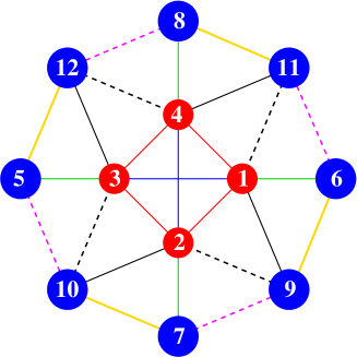
Figure 1: (Color online) Schematic structure of Mn12, same labeling as in Ref. Mazurenko et al., 2014. Mn${}^{\text{(IV)}}$ ions (1-4) are shown as red circles, Mn${}^{\text{(III)}}$ ions (5-12) as blue ones. An $S_{4}$ symmetry is assumed.

Since the discovery of the pronounced SMM-properties of Mn₁₂-acetate several groups developed parameterizations of the full spin-Hamiltonian. These data sets, of which the most prominent ones are given in Table 1, contain parameterizations of Heisenberg models and were put forward following various scientific reasonings. Earlier attempts assigned values of exchange interactions in analogy to smaller compounds with similar chemical bridges between the manganese ions. Later investigations combined for instance high-temperature series expansion with the evaluation of low-lying excitations seen in Inelastic Neutron Scattering (INS) experiments.Chaboussant et al. (2004) A necessary condition that has to be met by all parameterizations, is that the ground state has a total spin of $S=10$. The most recent DFT parameterization is also compatible with INS experiments.Mazurenko et al. (2014)

Table 1: Intra-molecular isotropic exchange interaction parameters (in meV) as suggested by various authors, compare Ref. Mazurenko et al., 2014. The spin labels are explained in Fig. 1.

No..	Bond (i-j) .	1-6 .	1-11 .	1-9 .	6-9 .	7-9 .	1-4 .	a 1-3
1	Jij (Ref. Mazurenko et al., 2014)	4.6	1.0	1.7	-0.45	-0.37	-1.55	-0.5
2	Jij (Ref. Boukhvalov et al., 2002)	4.8	1.37	1.37	-0.5	-0.5	-1.6	-0.7
3	Jij (Ref. Chaboussant et al., 2004)	5.8	5.3	5.3	0.5	0.5	0.7	0.7
4	Jij (Ref. Barbara et al., 1997)	7.4	1.72	1.72	0	0	-1.98	0
5	Jij (Ref. Regnault et al., 2002)	10.25	10.17	10.17	1.98	1.98	-0.69	-0.69

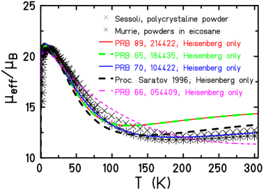
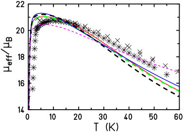
Figure 2: (Color online) Effective magnetic moment of Mn₁₂-acetate at $B=0.1$ T. Data of SessoliGatteschi and Sessoli (2003) and MurrieParois (2010) are given by symbols. Observables employing the Heisenberg part of parameterizations only are displayed by curves. The parameterizations correspond to those given in Table 1 from top to bottom.

Figure 2 shows the effective magnetic moment at a small external field of $B=0.1$ T as a function of temperature. Data of SessoliGatteschi and Sessoli (2003) and MurrieParois (2010) are given by symbols. For the theory curves only the Heisenberg part of the respective parametrizations is used. Since the Heisenberg model is SU(2) symmetric, a FTLM version employing total $\!\hbox{}\mathop{\vphantom{S}\smash{S}}\limits_{\sim}\!{}^{z}$ symmetry was used with $R=100$ and $N_{L}=120$ in this case.Schnack and Wendland (2010) One realizes that the gross structure of the magnetic moment (which is proportional to $\sqrt{\chi T}$) is achieved by all parameterizations especially at lower temperatures of $T\lessapprox 50$ K. A finer inspection shows that the maximum is at a too low temperature for all parameterizations, so that the experimental low-temperature data points are not met. For higher temperatures towards room temperature one notices that only one parameterizationChaboussant et al. (2004) (blue curve) closely follows the experimental data towards the paramagnetic limit. This is not astonishing since this parameterization was fitted to the high-temperature tail using a high-temperature series expansion. We conjecture that the somewhat too large effective magnetic moment of the DFT parameterizations, Refs. Mazurenko et al., 2014; Boukhvalov et al., 2002, at room temperature are related to the fact, that these parameterizations contain ferromagnetic interactions whereas a fit to the high-temperature behavior, Ref. Chaboussant et al., 2004, leads only to antiferromagnetic interactions, compare Table 1. In addition the antiferromagnetic interactions 1-11 and 1-9 are much stronger in Ref. Chaboussant et al., 2004.

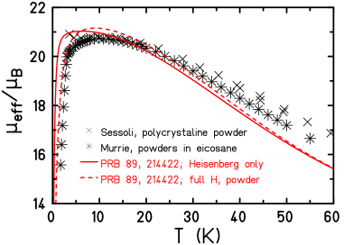
Figure 3: (Color online) Effective magnetic moment of Mn₁₂-acetate at $B=0.1$ T, same as Fig. 2. The dashed curve shows the result of a calculation employing the full Hamiltonian of Ref. Mazurenko et al., 2014. The powder average is performed over a regular grid of 20 directions on the unit sphere.Schnack (2009)

Using the recently developed FTLM for anisotropic systemsHanebaum and Schnack (2014) we could calculate the effective magnetic moment starting from the DFT parameterization of Ref. Mazurenko et al., 2014. Besides the Heisenberg terms of Table 1 this parameterization contains anisotropic Dzyaloshinskii-Moriya interactions as well as full $3\times 3$ anisotropy tensors for each manganese ion. It turns out that the additional terms improve the low-temperature data, compare Fig. 3. The maximum shifts towards the experimental position and the data points for smaller temperatures are much better approximated. None of the plain Heisenberg models could achieve such an improvement so far. For temperatures above 60 K the anisotropic terms are irrelevant.

IV Magnetization as function of applied field

The low-temperature magnetization usually provides strong fingerprints of the underlying spin-Hamiltonian for instance in the case of magnetization steps due to ground state level crossings. For Mn₁₂-acetate the magnetization shows even richer characteristics, since below the blocking temperature a magnetic hysteresis is observed.Sessoli et al. (1993b) This exciting physical property turns out to constitute a problem, when comparing to the theoretical equilibrium magnetization. Due to the long relaxation times, approximately 2800 hours at $T=2$ K,Gatteschi et al. (2006) the experimental values do not necessarily reflect equilibrium values. On the other hand, the theoretical evaluation of non-equilibrium observables for a full spin model of Mn₁₂-acetate is totally out of reach.

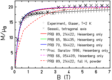
Figure 4: (Color online) Magnetization of Mn₁₂-acetate at $T=2$ K. Color code of curves as above. The dashed curve is evaluated for two field values per 1 T field interval only.

Figure 4 provides two experimental data sets as well as various theoretical curves. The data set of GlaserGlaser and Walleck was taken on a powder sample whereas the data set of SessoliGatteschi and Sessoli (2003) was taken on a single crystal with a field in direction of the tetragonal axis of the $S_{4}$ symmetric molecule. Both data sets coincide up to $B\approx 2.5$ T, then the magnetization along the tetragonal axis jumps whereas the powder signal smoothly increases with field. Already at this point it becomes clear that the measurements cannot reflect equilibrium properties, because the magnetization along the tetragonal axis, which is the easy axis of this strongly anisotropic molecule,Novak et al. (1995) cannot be the same as the powder averaged magnetization.

Interestingly, all theory curves that rest on Heisenberg model calculations agree with each other perfectly, which is due to the fact that all produce a $S=10$ ground state that is largely separated from excited levels. They also agree with the experimental magnetization up to a field of $B\approx 1$ T. Between 1 T and 2.7 T the experimental data points stay below the theoretical curves. Above $B\approx 2.7$ T theory and magnetization along the tetragonal axis meet again. The calculation for the full spin model of Mn₁₂-acetate as given in Ref. Mazurenko et al., 2014 yields a rather unexpected result: the powder-averaged magnetization stays well below all other theory curves (expected since anisotropic), but stays also well below both experimental curves (unexpected at least compared to the experimental powder data).

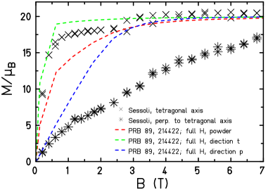
Figure 5: (Color online) Magnetization of Mn₁₂-acetate at $T=2$ K. The dashed curves are evaluated for two field values per 1 T field interval only. Direction $t=(0.0,-0.35682,0.93417)$, direction $p=(-0.35682,0.93417,0.0)$.

In the following we compare our results with the measurements of Ref. Gatteschi and Sessoli, 2003 along two different directions, along the tetragonal axis and perpendicular to that, i.e. somewhere in the $xy$-plane. Figure 5 presents three theory curves: one for the powder average and two along special directions. Direction $t=(0.0,-0.35682,0.93417)$ points roughly along the tetragonal axis (inclination of about $20^{\circ}$) and direction $p=(-0.35682,0.93417,0.0)$ lays in the $xy$-plane. Both theoretical curves show systematically larger magnetization values than the experiment. This could be for two reasons: either the experimental curves are not in equilibrium, which is possible at $T=2$ K where the relaxation time of Mn₁₂-acetate is long or the parameterization of Ref. Mazurenko et al., 2014 is still not yet optimal, i.e. the ${\mathbf{D}}$ tensors could be too weak, for instance. Nevertheless, the positive message is, that we can now calculate such curves and compare with experimental data. The theoretical costs, by the way, are still enormous. For the investigations shown in this article about 2 Mio. CPU hours on a supercomputer had to be used, since the FTLM procedure has to be completed twice for every field value and direction. Therefore, only a few field values have been used for the theoretical magnetization curves.

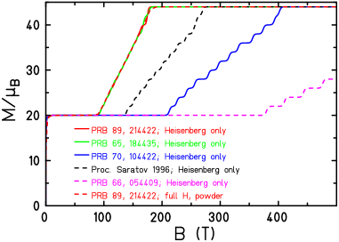
Figure 6: (Color online) High-field magnetization of Mn₁₂-acetate at $T=2$ K.

Finally we would like to present the high-field magnetization curves. As can be seen in Fig. 6 the various parameterizations lead to distinctive differences at high fields. The high-field magnetization could be and has been measured in megagauss experiments.Zvezdin et al. (1998) Interestingly, the magnetization data given in Ref. Zvezdin et al., 1998 show pronounced features, likely related to magnetization steps, between 180 T and 400 T which could be compatible with the parameterization of Ref. Chaboussant et al., 2004 (blue curve in Fig. 6). As realized already by the authors, this parameterization produces a sequence of level crossings between the $S=10$ ground manifold and the fully polarized state exactly in this field range.

V Heat capacity

Another observable that was measured very early in the history of Mn₁₂-acetate is the heat capacity.Gomes et al. (1998); Fernández et al. (1998); Luis et al. (2000) Figure 7 shows the experimental data of Ref. Gomes et al., 1998 for $B=0$ (top) and $B=0.3$ T (bottom). One notices that the heat capacity is rather large and grows steadily with temperature. This is due to a massive contribution from lattice vibrations (phonons) which grows like $T^{3}$. Therefore, heat capacity data of magnetic molecules are usually overwhelmed by phonon contributions above $T=5$ K.

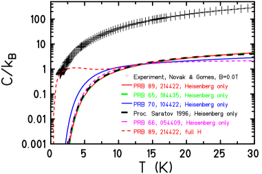
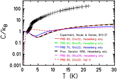
Figure 7: (Color online) Specific heat of Mn₁₂-acetate at $B=0$ (top) and $B=0.3$ T (bottom). Data taken from Ref. Gomes et al., 1998. Color code of curves as above. For $B=0.3$ T the calculation for the anisotropic spin model was averaged over 20 directions.

This fact becomes obvious when comparing the theoretical heat capacity data in Fig. 7 for the Heisenberg parameterizations at $B=0$. At low temperatures the theoretical values are two or more orders of magnitude smaller than the experimental ones. But for the calculation using the full anisotropic HamiltonianMazurenko et al. (2014) one notices that the low-temperature values agree very nicely. We think that this is due to a more smeared-out density of states at low energies in the anisotropic model whereas for Heisenberg systems these levels belong to highly degenerate multiplets which leads to a different, i.e. much smaller heat capacity.

Interestingly, a magnetic field of $B=0.3$ T has a similar effect. It smears out the density of states due to Zeeman splitting. Therefore even for the plain Heisenberg models the low-temperature heat capacity increases, but still does not agree with the experimental data. For the anisotropic spin-HamiltonianMazurenko et al. (2014) the low-temperature heat capacity does not change much and still agrees nicely with the experimental data. We conjecture that although the energy levels are moved around by the magnetic field, the overall structure of the density of states remains very similar.

Summarizing, the specific heat is well reproduced by the anisotropic spin-Hamiltonian of Ref. Mazurenko et al., 2014 for low-temperatures around 1 K.

VI Summary and Outlook

35 years after its synthesis and 22 years after the first measurementsSessoli et al. (1993a) of Mn₁₂-acetate the Finite-Temperature Lanczos Method puts us in a position to evaluate thermodynamic functions of really large magnetic molecules. It thus complements DFT calculations of such big systems in so far that one does no longer need to stop half way to an understanding of thermodynamic observables. The next major necessary step is now to develop tools for an evaluation of non-equilibrium properties of such big quantum spin systems.

References

- Liechtenstein et al. (1987) A. Liechtenstein, M. Katsnelson, V. Antropov, and V. Gubanov, J. Magn. Magn. Mater. 67, 65 (1987).
- Ruiz et al. (1997) E. Ruiz, P. Alemany, S. Alvarez, and J. Cano, J. Am. Chem. Soc. 119, 1297 (1997).
- Kortus et al. (2001) J. Kortus, C. S. Hellberg, and M. R. Pederson, Phys. Rev. Lett. 86, 3400 (2001).
- De Raedt et al. (2002) H. A. De Raedt, A. H. Hams, V. V. Dobrovitski, M. Al-Saqer, M. I. Katsnelson, and B. N. Harmon, J. Magn. Magn. Mater. 246, 392 (2002).
- Boukhvalov et al. (2003) D. W. Boukhvalov, E. Z. Kurmaev, A. Moewes, D. A. Zatsepin, V. M. Cherkashenko, S. N. Nemnonov, L. D. Finkelstein, Y. M. Yarmoshenko, M. Neumann, V. V. Dobrovitski, M. I. Katsnelson, A. I. Lichtenstein, B. N. Harmon, and P. Kögerler, Phys. Rev. B 67, 134408 (2003).
- Baruah et al. (2004) T. Baruah, J. Kortus, M. R. Pederson, R. Wesolowski, J. T. Haraldsen, J. L. Musfeldt, J. M. North, D. Zipse, and N. S. Dalal, Phys. Rev. B 70, 214410 (2004).
- Zaharko et al. (2008) O. Zaharko, J. Mesot, L. A. Salguero, R. Valentí, M. Zbiri, M. Johnson, Y. Filinchuk, B. Klemke, K. Kiefer, M. Mys’kiv, T. Strässle, and H. Mutka, Phys. Rev. B 77, 224408 (2008).
- Zartilas et al. (2013) S. Zartilas, C. Papatriantafyllopoulou, T. C. Stamatatos, V. Nastopoulos, E. Cremades, E. Ruiz, G. Christou, C. Lampropoulos, and A. J. Tasiopoulos, Inorg. Chem. 52, 12070 (2013).
- Kuepper et al. (2013) K. Kuepper, C. Derks, C. Taubitz, M. Prinz, L. Joly, J.-P. Kappler, A. Postnikov, W. Yang, T. V. Kuznetsova, U. Wiedwald, P. Ziemann, and M. Neumann, Dalton Trans. 42, 7924 (2013).
- Chiesa et al. (2013) A. Chiesa, S. Carretta, P. Santini, G. Amoretti, and E. Pavarini, Phys. Rev. Lett. 110, 157204 (2013).
- Silverstein et al. (2014) H. J. Silverstein, K. Fritsch, F. Flicker, A. M. Hallas, J. S. Gardner, Y. Qiu, G. Ehlers, A. T. Savici, Z. Yamani, K. A. Ross, B. D. Gaulin, M. J. P. Gingras, J. A. M. Paddison, K. Foyevtsova, R. Valenti, F. Hawthorne, C. R. Wiebe, and H. D. Zhou, Phys. Rev. B 89, 054433 (2014).
- Pedersen et al. (2014) K. S. Pedersen, G. Lorusso, J. J. Morales, T. Weyhermüller, S. Piligkos, S. K. Singh, D. Larsen, M. Schau-Magnussen, G. Rajaraman, M. Evangelisti, and J. Bendix, Angew. Chem. Int. Ed. 53, 2394 (2014).
- Sanz et al. (2014) S. Sanz, J. M. Frost, T. Rajeshkumar, S. J. Dalgarno, G. Rajaraman, W. Wernsdorfer, J. Schnack, P. J. Lusby, and E. K. Brechin, Chem. Eur. J. 20, 3010 (2014).
- Singh and Rajaraman (2014) S. K. Singh and G. Rajaraman, Chem. Eur. J. 20, 113 (2014).
- Kvashnin et al. (2015) Y. O. Kvashnin, O. Grånäs, I. Di Marco, M. I. Katsnelson, A. I. Lichtenstein, and O. Eriksson, Phys. Rev. B 91, 125133 (2015).
- Mazurenko et al. (2014) V. V. Mazurenko, Y. O. Kvashnin, F. Jin, H. A. De Raedt, A. I. Lichtenstein, and M. I. Katsnelson, Phys. Rev. B 89, 214422 (2014).
- Kortus et al. (2002) J. Kortus, T. Baruah, N. Bernstein, and M. R. Pederson, Phys. Rev. B 66, 092403 (2002).
- Boukhvalov et al. (2002) D. W. Boukhvalov, A. I. Lichtenstein, V. V. Dobrovitski, M. I. Katsnelson, B. N. Harmon, V. V. Mazurenko, and V. I. Anisimov, Phys. Rev. B 65, 184435 (2002).
- Chaboussant et al. (2004) G. Chaboussant, A. Sieber, S. Ochsenbein, H.-U. Güdel, M. Murrie, A. Honecker, N. Fukushima, and B. Normand, Phys. Rev. B 70, 104422 (2004).
- Gatteschi et al. (2006) D. Gatteschi, R. Sessoli, and J. Villain, Molecular Nanomagnets, Mesoscopic Physics and Nanotechnology (Oxford University Press, Oxford, 2006).
- Lis (1980) T. Lis, Acta Chrytallogr. B 36, 2042 (1980).
- Sessoli et al. (1993a) R. Sessoli, H. L. Tsai, A. R. Schake, S. Wang, J. B. Vincent, K. Folting, D. Gatteschi, G. Christou, and D. N. Hendrickson, J. Am. Chem. Soc. 115, 1804 (1993a).
- Sessoli et al. (1993b) R. Sessoli, D. Gatteschi, A. Caneschi, and M. A. Novak, Nature 365, 141 (1993b).
- Thomas et al. (1996) L. Thomas, F. Lionti, R. Ballou, D. Gatteschi, R. Sessoli, and B. Barbara, Nature 383, 145 (1996).
- Gomes et al. (1998) A. Gomes, M. Novak, R. Sessoli, A. Caneschi, and D. Gatteschi, Phys. Rev. B 57, 5021 (1998).
- Cornia et al. (2001) A. Cornia, M. Affronte, A. C. D. T. Gatteschi, A. G. M. Jansen, A. Caneschi, and R. Sessoli, J. Magn. Magn. Mater. 226, 2012 (2001).
- Gatteschi and Sessoli (2003) D. Gatteschi and R. Sessoli, Angew. Chem., Int. Edit. 42, 268 (2003).
- Schnalle and Schnack (2009) R. Schnalle and J. Schnack, Phys. Rev. B 79, 104419 (2009).
- Jaklič and Prelovšek (1994) J. Jaklič and P. Prelovšek, Phys. Rev. B 49, 5065 (1994).
- Jaklič and Prelovšek (2000) J. Jaklič and P. Prelovšek, Adv. Phys. 49, 1 (2000).
- Manthe and Huarte-Larranaga (2001) U. Manthe and F. Huarte-Larranaga, Chem. Phys. Lett. 349, 321 (2001).
- Long et al. (2003) M. W. Long, P. Prelovšek, S. El Shawish, J. Karadamoglou, and X. Zotos, Phys. Rev. B 68, 235106 (2003).
- Aichhorn et al. (2003) M. Aichhorn, M. Daghofer, H. G. Evertz, and W. von der Linden, Phys. Rev. B 67, 161103 (2003).
- Weiße et al. (2006) A. Weiße, G. Wellein, A. Alvermann, and H. Fehske, Rev. Mod. Phys. 78, 275 (2006).
- Prelovšek and Bonča (2013) P. Prelovšek and J. Bonča, “Strongly correlated systems, numerical methods,” (Springer, Berlin, Heidelberg, 2013) Chap. Ground State and Finite Temperature Lanczos Methods.
- Shannon et al. (2004) N. Shannon, B. Schmidt, K. Penc, and P. Thalmeier, Eur. Phys. J. B 38, 599 (2004).
- Zerec et al. (2006) I. Zerec, B. Schmidt, and P. Thalmeier, Phys. Rev. B 73, 245108 (2006).
- Schmidt et al. (2007) B. Schmidt, P. Thalmeier, and N. Shannon, Phys. Rev. B 76, 125113 (2007).
- Siahatgar et al. (2012) M. Siahatgar, B. Schmidt, G. Zwicknagl, and P. Thalmeier, New J. Phys. 14, 103005 (2012).
- Schnack and Wendland (2010) J. Schnack and O. Wendland, Eur. Phys. J. B 78, 535 (2010).
- Schnack and Heesing (2013) J. Schnack and C. Heesing, Eur. Phys. J. B 86, 46 (2013).
- Hanebaum and Schnack (2014) O. Hanebaum and J. Schnack, Eur. Phys. J. B 87, 194 (2014).
- Barra et al. (1997) A. L. Barra, D. Gatteschi, and R. Sessoli, Phys. Rev. B 56, 8192 (1997).
- Glaser et al. (2009) T. Glaser, M. Heidemeier, E. Krickemeyer, H. Bögge, A. Stammler, R. Fröhlich, E. Bill, and J. Schnack, Inorg. Chem. 48, 607 (2009).
- Glaser et al. (2010) T. Glaser, M. Heidemeier, H. Theil, A. Stammler, H. Bögge, and J. Schnack, Dalton Trans. 39, 192 (2010).
- Hoeke et al. (2012) V. Hoeke, K. Gieb, P. Müller, L. Ungur, L. F. Chibotaru, M. Heidemeier, E. Krickemeyer, A. Stammler, H. Bögge, C. Schröder, J. Schnack, and T. Glaser, Chem. Sci. 3, 2868 (2012).
- Farrell et al. (2013) A. R. Farrell, J. A. Coome, M. R. Probert, A. E. Goeta, J. A. K. Howard, M.-H. Lemee-Cailleau, S. Parsons, and M. Murrie, CrystEngComm 15, 3423 (2013).
- Barbara et al. (1997) B. Barbara, D. Gatteschi, A. A. Mukhin, V. V. Platonov, A. I. Popov, A. M. Tatsenko, , and A. K. Zvezdin, in Proceedings of Seventh International Conference on Megagauss Magnetic Field Generation and Related Topics (Sarov, 1996, 1997) p. 853.
- Regnault et al. (2002) N. Regnault, T. Jolicœur, R. Sessoli, D. Gatteschi, and M. Verdaguer, Phys. Rev. B 66, 054409 (2002).
- Parois (2010) P. Parois, The effect of pressure on clusters, chains and single-molecule magnets, Ph.D. thesis, Department of Chemistry, Faculty of Physical Sciences, University of Glasgow (2010).
- Schnack (2009) J. Schnack, Condens. Matter Phys. 12, 323 (2009).
- (52) T. Glaser and S. Walleck, Private communication.
- Novak et al. (1995) M. A. Novak, R. Sessoli, A. Caneschi, and D. Gatteschi, J. Magn. Magn. Mater. 146, 211 (1995).
- Zvezdin et al. (1998) A. K. Zvezdin, I. A. Lubashevskii, R. Z. Levitin, V. V. Platonov, and O. M. Tatsenko, Physics-Uspekhi 41, 1037 (1998).
- Fernández et al. (1998) J. F. Fernández, F. Luis, and J. Bartolomé, Phys. Rev. Lett. 80, 5659 (1998).
- Luis et al. (2000) F. Luis, F. L. Mettes, J. Tejada, D. Gatteschi, and L. J. de Jongh, Phys. Rev. Lett. 85, 4377 (2000).