Computational neuroanatomy: mapping cell-type densities in the mouse brain, simulations from the Allen Brain Atlas

Abstract

The Allen Brain Atlas (ABA) of the adult mouse consists of digitized expression profiles of thousands of genes in the mouse brain, co-registered to a common three-dimensional template (the Allen Reference Atlas). This brain-wide, genome-wide data set has triggered a renaissance in neuroanatomy. Its voxelized version (with cubic voxels of side 200 microns) can be analyzed on a desktop computer using MATLAB. On the other hand, brain cells exhibit a great phenotypic diversity (in terms of size, shape and electrophysiological activity), which has inspired the names of some well-studied cell types, such as granule cells and medium spiny neurons. However, no exhaustive taxonomy of brain cells is available. A genetic classification of brain cells is under way, and some cell types have been characterized by their transcriptome profiles. However, given a cell type characterized by its transcriptome, it is not clear where else in the brain similar cells can be found. The ABA can been used to solve this region-specificity problem in a data-driven way: rewriting the brain-wide expression profiles of all genes in the atlas as a sum of cell-type-specific transcriptome profiles is equivalent to solving a quadratic optimization problem at each voxel in the brain. However, the estimated brain-wide densities of 64 cell types published recently were based on one series of co-registered coronal in situ hybridization (ISH) images per gene, whereas the online ABA contains several image series per gene, including sagittal ones. In the presented work, we simulate the variability of cell-type densities in a Monte Carlo way by repeatedly drawing a random image series for each gene and solving optimization problems. This yields error bars on the region-specificity of cell types.
Prepared for the International Conference on Mathematical Modeling in Physical Sciences, 5th-8th June 2015, Mykonos Island, Greece.

1 Introduction

The Allen Brain Atlas (ABA, [1, 2]) put neuroanatomy on a genetic basis by releasing voxelized, in situ hybridization data for the expression of the entire genome in the mouse brain (www.mouse-brain.org). These data were co-registered to the Allen Reference Atlas of the mouse brain (ARA, [3]). About 4,000 genes of special neurobiological interest were proritized. For these genes an entire brain was sliced coronally and processed (giving rise to the coronal ABA). For the rest of the genome the brain was sliced sagitally, and only the left hemisphere was processed (giving rise to the sagittal ABA).
From a computational viewpoint, gene-expression data from the the ABA can be studied collectively, thousands of genes at a time. Indeed the collective behaviour of gene-expression data is crucial for the analysis of [4], in which the brain-wide correlation between the ABA and cell-type-specific microarray data was studied. These microarray data characterize the transcriptome of $64$ different cell types, microdissected from the mouse brain, and collated in [5]. However, for a given cell characterized in this way, it is not known where other cells of the same type are located in the brain. A linear model was proposed in [4, 6, 7] (see also [8, 9, 10]), and used to estimate the region-specificity of cell types by linear regression with positivity constraint. The model was fitted using the coronal ABA only, which allowed to obtain brain-wide results. However, this restriction implies that only one ISH expression profile per gene was used to fit the model. This poses the problem of the error bars on the results of the model.

2 Spatial densities of cell types in the mouse mouse brain from the ABA and transcriptome profiles

Since all the ISH data in the ABA were co-registered to the voxelized ARA, so that data for the sagittal and coronal atlas can be treated computationally in the same way. However, the ABA does not specify from which cell type(s) the expression of each gene comes.
Gene expression energies from the Allen Brain Atlas. In the ABA, the adult mouse brain is partitioned into $V=49,742$ cubic voxels of side 200 microns, to which ISH data are registered [1, 2, 3] for thousands of genes. For computational purposes, these gene-expression data can be arranged into a voxel-by-gene matrix. For a cubic labeled $v$, the expression energy [1, 2] of the gene $g$ is a weighted sum of the greyscale-value intensities evaluated at the pixels intersecting the voxel:

$$E(v,g)={\mathrm{expression\;energy\;of\;gene\;labeled\;}}g\;{\mathrm{in\;voxel\;labeled\;}}v,$$ (1)

The analysis of [4] is restricted to digitized image series from the coronal ABA, for which the entire mouse brain was processed in the ABA pipeline (whereas only the left hemisphere was processed for the sagittal atlas).
Cell-type-specific transcriptomes and density profiles. On the other hand, the cell-type-specific microarray reads collated in [5] (for $T=64$ different cell-type-specific samples studied in [11, 12, 13, 14, 15, 16, 17, 18]) can be arranged in a type-by-gene matrix denoted by $C$, such that

$$C(t,g)={\mathrm{expression\;of\;gene\;labeled\;}}g\;{\mathrm{in\;cell\;type\;labeled\;}}t,$$ (2)

and the columns are arranged in the same order as in the matrix $E$ of expression energies defined in Eq. 1.
We proposed the following linear model in [4] for a voxel-based gene-expression atlas in terms of the transcriptome profiles of individual cell types and their spatial densities:

$$E(v,g)=\sum_{t}\rho_{t}(v)C(t,g)+{\mathrm{Residual}}(v,g),$$ (3)

where the index $t$ denotes labels cell type, and $\rho_{t}(v)$ denotes its (unknown) density at voxel labeled $v$. The values of the cell-type-specific density profiles were computed in [4] by minimizing the value of the residual term over all the (positive) density profiles, which amounts to solving a quadratic optimization problem (with positivity constraint) at each voxel. These computations can be reproduced on a desktop computer using the MATLAB toolbox Brain Gene Expression Analysis (BGEA) [19, 20]. For other applications of the toolbox see [21] (marker genes of brain regions), [22, 23] for co-expression properties of some autism-related genes, and [24] for computations of stereotactic coordinates).

3 Monte Carlo simulation of variability of spatial densities of cell types

The optimization procedure in our model is deterministic. On the other hand, decomposing the density of a cell type into the sum of its mean and Gaussian noise is a difficult statistics problem (see [25]). Some error estimates on the value of $\rho_{t}(v)$ were obained in [4] using sub-sampling techniques (i.e. sub-sampling the data repeatedly by keeping only a random 10% of the coronal ABA). This induced a ranking of the cell types based on the stability of the results against sub-sampling. However, the 10 % fraction is arbitrary (even though it is close to the fraction of the genome covered by our coronal data set).

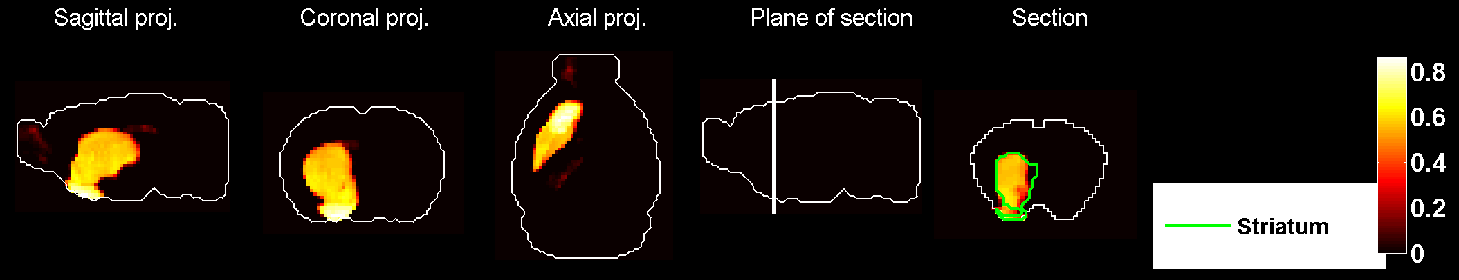
Figure 1: Heat map of the average density of cell types in the left hemisphere, $\langle\rho_{t}(v)\rangle$, defined in Eq. 4, for medium spiny neurons, labeled $t=16$ in our data set. The restriction to the left hemisphere comes from the use we made of sagittal image series, which cover the left hemisphere only.

In the present work we simulated the variability of the spatial density of cell types by integrating the digitized sagittal image series into the data set. For gene labeled $g$, the ABA provides $N(g)$ expression profiles, where $N(g)$ is the number of image series in the ABA for this gene. Hence, instead of just one voxel-by-gene matrix, the ABA gives rise to a family of $\prod_{g=1}^{G}N(g)$ voxel-by-gene matrices, with voxels belonging to the left hemisphere. A quantity computed from the coronal ABA can be recomputed from any of these matrices, thereby inducing a distribution for this quantity. This is a finite but prohibitively large number of computations, so we took a Monte Carlo approach based on $R$ random choices of images series, described by the following pseudo-code:
for all $i$ in $[1..R]$
1. for all $g$ in [1..G], choose an image series labeled by the integer $n_{i}(g)$ in $[1..N(g)]$;
2. construct the matrix $E_{[i]}$ with entries $E_{[i]}(v,g)=E^{(n_{i}(g))}(v,g)$,
3. estimate the density of cell type labeled $t$ using this matrix, call the result $\rho_{t,[i]}$;
end
The larger $R$ is, the more precise the estimates for the distribution of the spatial density of cell types will be. The only price we have to pay for th e integration of the sagittal ABA is the restriction of the results to the left hemisphere in step 2 of the pseudo-code.

4 Anatomical analysis of results

The average density across random draws of image series for cell type labeled $t$ reads:

$$\langle\rho_{t}(v)\rangle=\frac{1}{R}\sum_{i=1}^{R}\rho_{t,[i]}(v).$$ (4)

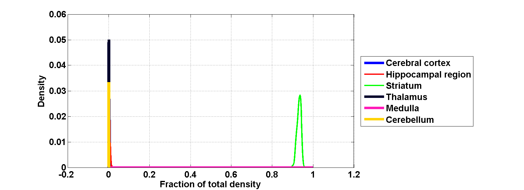
Figure 2: Estimated probability densities of fractions of density agglomerated in a few regions of the coarsest versions of the ARA (see Eq. 5), for medium spiny neurons, labeled $t=16$, based on $R=1000$ random draws. The right-most peak, corresponding to the striatum, is well-decoupled from the others, furthermore the other peaks are all centered close to zero (making most of them almost invisible). Medium spiny neurons have $93(\pm 3)$ percent of their densities supported in the striatum, without any region gathering more than 5 percent of the signal in any of the random draws.

A heat map of this average for medium spiny neurons (extracted from the striatum) is presented on Fig. 1. It is optically very similar to the (left) striatum, which allows the model to predict that medium spiny neurons are specific to the striatum (which confirms prior neurobiological knowledge and therefore serves as a proof of concept for the model).
To compare the results to classical neuroanatomy, we can group the voxels by region according to the ARA. Since the number of cells of a given type in an extensive quantity, we compute the fraction of the total density contributed by a given brain region denoted by $V_{r}$ (see the legend of Fig. 2 for a list of possible values of $V_{r}$):

$$\phi_{r,[i]}(t)=\frac{1}{\sum_{v\in\mathrm{left\;hemisphere}}\rho_{[i],t}(v)}\sum_{v\in V_{r}}\rho_{t,[i]}(v).$$ (5)

We can plot the distribution of these $R$ values for a given cell type and all brain regions (see Fig. 1 for medium spiny neurons, which gives rise to the best-decoupled right-most peak in the distribution of simulated densities). Moreover, we estimated the densities of the contribution of each region in the coarsest version of the ARA to the total density of each cell type in the data set. For most cell types, this confirms the ranking of cell types by stability obtained in [4], but based on error bars obtained from the same set of genes in every fitting of the model (see the accompanying preprint [26] for exhaustive results for all cell types in the panel). The most stable results against sub-sampling tend to correspond to cell types for which the anatomical distribution of results is more peaked. The present analysis can be repeated when the panel of cell-type-specific microarray expands.

Microarray data were made available by Ken Sugino, Benjamin Okaty and Sacha B. Nelson. The Allen Atlas data were analysed under the guidance of Michael Hawrylycz and Lydia Ng. This work is supported by the Research Development Fund and the Research Conference Fund of Xi’an Jiaotong–Liverpool University.

References

References

- [1] E.S. Lein et al. (2007), Genome-wide atlas of gene expression in the adult mouse brain, Nature 445, 168–176.
- [2] L. Ng, et al. (2009), An anatomic gene expression atlas of the adult mouse brain, Nature Neuroscience 12, 356–362.
- [3] H.-W. Dong (2007), The Allen reference atlas: a digital brain atlas of the C57BL/6J male mouse, Wiley.
- [4] P. Grange, J.W. Bohland, B.W. Okaty, K. Sugino. H. Bokil, S.B. Nelson, L. Ng, M. Hawrylycz and P.P. Mitra, Cell-type–based model explaining coexpression patterns of genes in the brain, Proceedings of the National Academy of Sciences 2014 111 (14) 5397–5402.
- [5] B.W. Okaty, K. Sugino and S.B. Nelson (2011), A Quantitative Comparison of Cell-Type-Specific Microarray Gene Expression Profiling Methods in the Mouse Brain, PLoS One 6(1).
- [6] P. Grange, M. Hawrylycz and P.P. Mitra, Cell-type-specific microarray data and the Allen atlas: quantitative analysis of brain-wide patterns of correlation and density, [arXiv:1303.0013].
- [7] P. Grange, J.W. Bohland, B.W. Okaty, K. Sugino. H. Bokil, S.B. Nelson, L. Ng, M. Hawrylycz and P.P. Mitra, Cell-type-specific transcriptomes and the Allen Atlas (II): discussion of the linear model of brain-wide densities of cell types, [arXiv:1402.2820] .
- [8] Y. Ko, S.A. Ament, J.A. Eddy, J. Caballero, J.C. Earls, L. Hood and N.D. Price (2013), Cell-type-specific genes show striking and distinct patterns of spatial expression in the mouse brain, Proceedings of the National Academy of Sciences, 110 (8), 3095–3100.
- [9] P.P.C. Tan, L. French and P. Pavlidis (2013), Neuron-enriched gene expression patterns are regionally anti-correlated with oligodendrocyte-enriched patterns in the adult mouse and human brain, Frontiers in Neuroscience, 7.
- [10] R. Li, W. Zhang, and S. Ji (2014), Automated identification of cell-type-specific genes in the mouse brain by image computing of expression patterns, BMC bioinformatics, 15(1), 209.
- [11] K. Sugino et al. (2005), Molecular taxonomy of major neuronal classes in the adult mouse forebrain, Nature Neuroscience 9, 99–107.
- [12] C.Y. Chung et al. (2005), Cell-type-specific gene expression of midbrain dopaminergic neurons reveals molecules involved in their vulnerability and protection, Hum. Mol. Genet. 14: 1709–1725.
- [13] P. Arlotta et al. (2005), Neuronal subtype-specific genes that control corticospinal motor neuron development in vivo, Neuron 45 207–221.
- [14] M.J. Rossner et al. (2006), Global transcriptome analysis of genetically identified neurons in the adult cortex, J. Neurosci. 26(39) 9956–66.
- [15] M. Heiman et al. (2008), A translational profiling approach for the molecular characterization of of CNS cell types, Cell 135: 738–748.
- [16] J.D. Cahoy et al. (2008), A transcriptome database for astrocytes, neurons, and oligodendrocytes: a new resource, for understanding brain development and function. J. Neurosci., 28(1) 264–78.
- [17] J.P. Doyle et al. (2008), Application of a translational profiling approach for the comparative analysis of CNS cell types, Cell 135(4) 749–62.
- [18] B.W. Okaty et al. (2009), Transcriptional and electrophysiological maturation of neocortical fast-spiking GABAergic interneurons, J. Neurosci. (2009) 29(21) 7040–52.
- [19] P. Grange, M. Hawrylycz and P.P. Mitra (2013), Computational neuroanatomy and co-expression of genes in the adult mouse brain, analysis tools for the Allen Brain Atlas, Quantitative Biology, 1(1): 91–100. (DOI) 10.1007/s40484-013-0011-5.
- [20] P. Grange, J.W. Bohland, M. Hawrylycz and P.P. Mitra (2012), Brain Gene Expression Analysis: a MATLAB toolbox for the analysis of brain-wide gene-expression data, [arXiv:1211.6177].
- [21] P. Grange and P.P. Mitra (2012), Computational neuroanatomy and gene expression: optimal sets of marker genes for brain regions, IEEE, in CISS 2012, 46th annual conference on Information Science and Systems (Princeton).
- [22] I. Menashe, P. Grange, E.C. Larsen, S. Banerjee-Basu and P.P. Mitra (2013), Co-expression profiling of autism genes in the mouse brain, PLoS computational biology, 9(7), e1003128.
- [23] P. Grange, I. Menashe and M. Hawrylycz (2015), Cell-type-specific neuroanatomy of cliques of autism-related genes in the mouse brain, Frontiers in Computational Neuroscience, 9, 55.
- [24] P. Grange and P.P. Mitra (2011), Algorithmic choice of coordinates for injections into the brain: encoding a neuroanatomical atlas on a grid, [’arXiv:1104.2616].
- [25] N. Meinshausen (2013), Sign-constrained least squares estimation for high-dimensional regression, Electronic Journal of Statistics, 7, 1607–1631.
- [26] P. Grange, Cell-type-specific computational neuroanatomy, simulations from the sagittal and coronal Allen Brain Atlas, [arXiv:1505.06434].