Entanglement dynamics of two interacting qubits under the influence of local dissipation

Abstract

We investigate the dynamics of entanglement given by the concurrence of a two-qubit system in the non-Markovian setting. A quantum master equation is derived which is solved in the eigen basis of the system Hamiltonian for $X$-type initial states. A closed formula for time evolution of concurrence is presented for a pure state. It is shown that under the influence of dissipation that non-zero entanglement is created in unentangled two qubit states which decay in the same way as pure entangled states. We also show that under real circumstances, the decay rate of concurrence is strongly modified by the non-Markovianity of the evolution.

I Introduction

The important ingredient for quantum computation and information processing is the presence of coherent superpositions. A single isolated two-level system can be prepared in a coherent superposition of $|0\rangle$ and $|1\rangle$ states, and the manipulation of such states leads to new possibilities for storage and processing of information Nielsen . In contrast to the ideal isolated case, the interactions of real quantum systems with their environment lead to the loss of these coherent superpositions, in other words, decoherence. However, the more realistic case would be manipulation of many qubits. Coherent superposition of such states leads to the concept of entanglement, which forms a precious resource for quantum computation and information. The fragility of entanglement is due to the coupling between a quantum system and its environment; such a coupling leads to decoherence, the process by which information is degraded MaxSc ; zurek2 . In fact, decoherence is one of the main obstacles for the preparation, observation, and implementation of multi-qubit entangled states. The intensive work on quantum information and computing in recent years has tremendously increased the interest in exploring and controlling decoherence effects nat1 ; milb2 ; QA ; CJ ; zurek ; diehl ; verst ; weimer . In this work we address the problem where each of the two qubits are dissipatively coupled to a local bosonic bath; in quantum optical sense it would mean that both the two-level systems are subject to spontaneous emission and would imply there exist relaxation between the excited state to ground state. Dissipation can assist the generation of entanglement MPl ; Beige ; PHoro that can be used for various quantum information processing. For example, F. Verstraete et al verst have shown that dissipation can be used as a resource for the universal quantum computation without any coherent dynamics needed to implement it. Contrary to other methods, entanglement generation by dissipation does not require the preparation of a system in a particular input state and exists, in principle, for an arbitrary long time. These features make dissipative methods inherently stable against weak random perturbations, with the dissipative dynamics stabilizing the entanglement.

The effects on system due to environment can be classified into the process with memory (Non-Markovian) and without memory (Markovian) effects (Pet, ; RF1, ; RF2, ; RF3, ; RF4, ; self, ). In case of Markovian processes, the environment acts as a sink for the system information; the system of interest loses information into the environment and this lost information plays no role in the dynamics of the system. However, due to memory effects in case of non-Markovian dynamics, the information lost by the system during the interaction with the environment will return back to the system at later time. This makes the non-Markovian dynamics complicated. Understanding the nature of non-Markovian dynamics is naturally a very important topic for quantum information science, where the aim is to control a quantum system for use in technological applications Terhal ; Ban ; Wolf ; Cirac . In general, three time scales in an open system exist to characterize non-Markovian dynamics: (i) the time scale of the system (ii) the time scale of the bath given by the bandwidth of bath spectral density (iii) the mutual time scale arising from the coupling between the system and the bath. It is usually believed that non-Markovian effects strongly rely on the relations among these different time scales 27 ; 30 ; 31 .

In this paper we derive a quantum master equation for interacting qubits with local dissipation. The equation is derived utilizing the completeness of the eigen basis of the Hamiltonian representing the interacting qubits. The time evolution of the density matrix turns out to be the sum of the time evolution corresponding to individual qubits with no cross terms. Next we solve this master equation for $X$-type states with the assumption that individual baths have the same properties. The main content of this paper will remain however the same as for other kind of states and assuming different bath correlation functions for each bath. The different bath correlation functions can give rise to different time scales in the dynamics and is treated separately. Next we identify different regimes of dynamics (Markovian and non-Markovian) and show that under non-Markovian regimes of the dynamics, there exists finite entanglement in an initially unentangled state. This entanglement decay in the same way as the pure state entanglement and we find that the decay rate of entanglement is strongly modified by the non-Markovian behavior.

The rest of the paper is organized as follows: In section II, we introduce the model Hamiltonian and derive the quantum master equation. In the past related works Pet ; RF1 ; RF2 ; RF3 ; RF4 , non-interacting qubits have been considered. These qubits are then coupled to a common bath. However, in this paper, we consider qubits interacting through isotropic Heisenberg interaction which is a general kind of interaction in condensed matter physics. In section III, we solve the quantum master equation in the eigen-basis of the system Hamiltonian for a general class of initial quantum states under the assumption that the bath correlation function decay in the same way.In section IV we give the decay of entanglement of certain $X$-type state. Finally we conclude in section V with the remarks of wider context of our results.

II Master equation for local dissipation

In this section we will first derive master equation for the reduced density matrix of the system which govern the dynamics of the system. We consider two qubits represented by spin-$\frac{1}{2}$ particles or two level atoms coupled to each other via isotropic Heisenberg interaction. The qubits are subject to local dissipation through a coupling with a bosonic bath. The Hamiltonian of the two qubit system is

$$H_{s} = J\overrightarrow{\sigma}_{1}.\overrightarrow{\sigma}_{2}$$ (1)

$$= J[\sigma_{1}^{+}\sigma_{2}^{-}+\sigma_{1}^{-}\sigma_{2}^{+}+\sigma_{1}^{z}\sigma_{2}^{z}],$$

where $\sigma_{i}^{\pm}=\frac{\sigma_{i}^{x}\pm i\sigma_{i}^{y}}{2}$. $J$ represents the energy scale of the system. The Hamiltonian $H_{s}$ can be diagonalized exactly i.e. $H_{s}|\psi_{i}\rangle=\epsilon_{i}|\psi_{i}\rangle$ where $|\psi_{i}\rangle$’s are the eigenstates of the Hamiltonian $H_{s}$ with the eigen energies $\epsilon_{i}$ and are given below (with notation $|0\rangle=|\uparrow\rangle$ and $|1\rangle=|\downarrow\rangle$ ):

$$\epsilon_{1}=J; ~{}~{}~{}\psi_{1}=|00\rangle$$

$$\epsilon_{2}=0; ~{}~{}~{}\psi_{2}=\frac{1}{\sqrt{2}}[|01\rangle+|01\rangle]$$

$$\epsilon_{3}=-2J; ~{}~{}~{}\psi_{3}=\frac{1}{\sqrt{2}}[|01\rangle-|01\rangle]$$

$$\epsilon_{4}=J; ~{}~{}~{}\psi_{4}=|11\rangle.$$

We write the total Hamiltonian (system+bath)

$$H=H_{s}+H_{B}+H_{I}$$ (2)

where $H_{B}$ is the Hamiltonian for the bath

$$H_{B}=\sum_{i=1}^{2}\sum_{k}\omega_{k}b_{ik}^{\dagger}b_{ik},$$ (3)

and the dissipative interaction of the system with bath is represented by the Hamiltonian

$$H_{I} = \sum_{i=1}^{2}\sigma_{i}^{x}\sum_{k}[g_{ik}b_{ik}+g_{ik}^{\star}b_{ik}^{\dagger}]$$ (4)

$$= \sum_{i=1}^{2}\sigma_{i}^{x}(B_{i}+B_{i}^{\dagger})$$

where $B_{i}=\sum_{k}g_{ik}b_{ik}$. Let $\tilde{O}(t)=e^{iH_{o}t}Oe^{-iH_{o}t}$ represent an operator defined in interaction picture with respect to system and bath ($H_{o}=H_{s}+H_{B}$), we can therefore write $H_{I}$ in the interaction picture under rotating wave approximation as

$$\tilde{H}_{I}(t)=\sum_{i=1}^{2}[\tilde{\sigma}_{i}^{+}(t)\tilde{B}_{i}(t)+\tilde{\sigma}_{i}^{-}(t)\tilde{B}_{i}^{\dagger}(t)].$$ (5)

The time evolution of the system operators can be evaluated using the eigen basis of the system Hamiltonian $H_{s}$ as

$$\sigma_{1}^{+}(\tau) = \sum_{i,j=1}^{4}\!\!\!P_{ij}\langle\psi_{i}|\sigma_{1}^{+}\otimes I_{2}|\psi_{j}\rangle\exp[i(\epsilon_{i}-\epsilon_{j})\tau]$$ (6)

$$\sigma_{2}^{+}(\tau) = \sum_{i,j=1}^{4}\!\!\!P_{ij}\langle\psi_{i}|I_{1}\otimes\sigma_{2}^{+}|\psi_{j}\rangle\exp[i(\epsilon_{i}-\epsilon_{j})\tau]$$ (7)

where $P_{ij}=|\psi_{i}\rangle\langle\psi_{j}|$ is the projection operator $P_{ij}P_{jk}=P_{ik}$ and $\sum_{i}P_{ii}=I$. In interaction picture, the time evolution of the total density matrix (system and bath) $\rho_{T}(t)$ is given by the von Neuman-Liouville equation as

$$\frac{d\tilde{\rho}_{T}(t)}{dt}=-i[\tilde{H}_{I}(t),\tilde{\rho}_{T}(t)].$$ (8)

Here we have used $\hbar=1$. We can formally integrate equation (8) and write its solution as:

$$\tilde{\rho}_{T}(t)=\tilde{\rho}_{T}(0)-i\int_{0}^{t}\!\!ds[\tilde{H}_{I}(s),\tilde{\rho}_{T}(s)].$$ (9)

Subsituting this solution back into the commutator of equation (8), we get upto second order the following equation:

$$\frac{d\tilde{\rho}_{T}(t)}{dt}= - i\left[\tilde{H}_{I}\left(t\right),\tilde{\rho}_{T}\left(0\right)\right]$$ (10)

$$- \int\nolimits_{0}^{t}ds\left[\tilde{H}_{I}\left(t\right),\left[\tilde{H}_{I}\left(s\right),\tilde{\rho}_{T}\left(s\right)\right]\right].$$

The solution of the above equation depends on the initial conditions of total density operator. We consider an initially uncorrelated situation, i.e $\rho_{T}(0)=\rho_{s}(0)\otimes\rho_{B}$, where $\rho_{s}$ and $\rho_{B}$ are respectively the density operators for the system and bath. Tracing over the bath degrees of freedom and assuming that $tr_{B}[\tilde{H}_{I}(t)\rho_{B}]=0$, we get the following time non-local master equation for the reduced density matrix:

$$\frac{d\tilde{\rho}_{s}(t)}{dt}=-\int_{0}^{t}\!\!\!ds~{}tr_{B}[\tilde{H}_{I}(t),[\tilde{H}_{I}(s),\tilde{\rho}_{T}(s)]].$$ (11)

As the bath degree of freedom are infinite so that the influence of the system on the bath is small in the weak system-bath coupling case. As a cosequence, we write the total density operator $\tilde{\rho}_{T}(s)=\tilde{\rho}_{s}(s)\otimes\rho_{B}+\mathcal{O}(\tilde{H_{I}})$ within the second order perturbation of system-bath coupling Pet ; HJ ; HFPB ; HPB ; MS ; EF . The replacement of total density matrix $\tilde{\rho}_{T}(s)$ with an uncorrelated state $\tilde{\rho}_{s}(s)\otimes\rho_{B}$ is called as Born approximation. Therefore, under Born approximation we write

$$\frac{d\tilde{\rho}_{s}(t)}{dt}=-\int_{0}^{t}\!\!\!ds~{}tr_{B}[\tilde{H}_{I}(t),[\tilde{H}_{I}(s),\tilde{\rho}_{s}(s)\otimes\rho_{B}]].$$ (12)

The above equation is in a form of delayed integro-differential equation and is therefore a time non-local master equation. Replacing $\tilde{\rho}_{s}(s)$ with $\tilde{\rho}_{s}(t)$ in this equation Pet ; HFPB ; HPB we get time-local master equation:

$$\frac{d\tilde{\rho}_{s}(t)}{dt}=-\int_{0}^{t}\!\!\!ds~{}tr_{B}[\tilde{H}_{I}(t),[\tilde{H}_{I}(s),\tilde{\rho}_{s}(t)\otimes\rho_{B}]].$$ (13)

Assuming the bath in the vacuum state initially, i.e $\rho_{B}=|0\rangle\langle 0|$; using the form of the $\tilde{H}_{I}(t)$, we arrive at the following equation:

$$\frac{d\tilde{\rho}_{s}(t)}{dt}=\mathcal{L}_{1}[\tilde{\rho}_{s}(t)]+\mathcal{L}_{2}[\tilde{\rho}_{s}(t)].$$ (14)

This forms a non-trivial result. The master equations contains sums of $\mathcal{L}_{i}$ for each qubit and no cross terms with different $\mathcal{L}_{i}$’s. This result is the same as that for the non-interacting qubits. Here we have ($i=1,2$)

$$\!\!\!\!\!\!\!\!\!\mathcal{L}_{i}(\tilde{\rho}_{s}(t)) = \int_{0}^{t}\!\!\!ds\{\Phi_{i}(t-s)[\tilde{\sigma}_{i}^{-}(s)\tilde{\rho}_{s}(t),\tilde{\sigma}_{i}^{+}(t)]$$ (15)

$$~{}~{}~{}~{}~{}~{}+\Phi_{i}^{\dagger}(t-s)[\tilde{\sigma}_{i}^{-}(t),\tilde{\rho}_{s}(t)\tilde{\sigma}_{i}^{+}(s)]\}$$

and the bath correlation function is defined as

$$\Phi_{i}(t-s) = \langle B_{i}(t-s)B_{i}^{\dagger}\rangle_{0}$$ (16)

$$= \sum_{k}|g_{ik}|^{2}\exp[-i\omega_{k}(t-s)].$$

Next we revert back to the Schr$\ddot{o}$dinger picture with a change in variable $\tau=t-s$, we write

$$\frac{d\rho_{s}(t)}{dt} = -i[H_{s},\rho_{s}(t)]$$ (17)

$$+\sum_{i=1}^{2}\int_{0}^{t}d\tau\left[\Phi_{i}(\tau)[\sigma_{i}^{-}(-\tau)\rho_{s}(t),\sigma_{i}^{+}]\right.$$

$$~{}~{}~{}~{}~{}~{}~{}~{}~{}~{}~{}~{}~{}~{}\left.+\Phi_{i}^{\dagger}(\tau)[\sigma_{i}^{-},\rho_{s}(t)\sigma_{i}^{+}(-\tau)]\right].$$

This represents the quantum master equation in the Schr$\ddot{o}$dinger picture. The solution of the above master equation depends on the type of initial states. In the next section we find its solution for general $X$-type initial states.

III Solution of Master equation

In order to obtain the dynamics of entanglement of our two qubit system, we assume that the qubits are initially prepared in an X state TingYU :

$$\rho_{s}(0)=\left[\begin{array}[]{cccc}u(0)&0&0&w(0)\\ 0&x_{1}(0)&y(0)&0\\ 0&y^{\star}(0)&x_{2}(0)&0\\ w^{\star}(0)&0&0&v(0)\end{array}\right]$$ (18)

where we have used the standard basis $\{|00\rangle,|01\rangle,|10\rangle,|11\rangle\}$. Since the normalization and positivity of $\rho_{s}(0)$ i.e, $tr(\rho_{s}(0))=1$ and $\rho_{s}(0)>0$, the matrix elements $u,x_{1},x_{2},v$ are non-negative parameters with $u+x_{1}+x_{2}+v=1$, $\sqrt{uv}\geq|w|$, and $\sqrt{x_{1}x_{2}}\geq|y|$. We can use more general forms of density matrix with all elements non-zero, this makes the master equation intractable analytically. Next we express the X state $\rho_{s}(0)$ in the eigen basis of $H_{s}$ as

$$\rho_{s}(0) = a(0)|\psi_{1}\rangle\langle\psi_{1}|+b(0)|\psi_{2}\rangle\langle\psi_{2}|+e(0)|\psi_{3}\rangle\langle\psi_{3}|$$ (19)

$$+~{}d(0)|\psi_{4}\rangle\langle\psi_{4}|+c(0)|\psi_{1}\rangle\langle\psi_{4}|+c^{\star}(0)|\psi_{4}\rangle\langle\psi_{1}|$$

$$+~{}h(0)|\psi_{2}\rangle\langle\psi_{3}|+h^{\star}(0)|\psi_{3}\rangle\langle\psi_{2}|$$

where the various parameters of the density operator in the eigen basis of $H_{s}$ are related to the parameters in the standard basis in the following way: $a(0)=u(0)$, $b(0)=\frac{1}{2}[x_{1}(0)+x_{2}(0)+y(0)+y^{\star}(0)]$,  $e(0)=\frac{1}{2}[x_{1}(0)+x_{2}(0)-y(0)-y^{\star}(0)]$,  $h(0)=\frac{1}{2}[x_{1}(0)-x_{2}(0)-y(0)+y^{\star}(0)]$, $d(0)=v(0)$,  $c(0)=w(0)$. Next we see that the form of the density matrix is invariant during the time evolution generated by the quantum master equation. Therefore we can the density matrix at time $t$ as

$$\rho_{s}(t) = a(t)|\psi_{1}\rangle\langle\psi_{1}|+b(t)|\psi_{2}\rangle\langle\psi_{2}|+e(t)|\psi_{3}\rangle\langle\psi_{3}|$$ (20)

$$+~{}d(t)|\psi_{4}\rangle\langle\psi_{4}|+c(t)|\psi_{1}\rangle\langle\psi_{4}|+c^{\star}(t)|\psi_{4}\rangle\langle\psi_{1}|$$

$$+~{}h(t)|\psi_{2}\rangle\langle\psi_{3}|+h^{\star}(t)|\psi_{3}\rangle\langle\psi_{2}|.$$

In order to find the time evolution equations of the various parameters involved in equation (20) we assume that the bath correlation functions have the same form

$$\Phi_{i}(s)=\frac{\Gamma_{i}\lambda}{2}e^{-\lambda|s|}$$ (21)

where $\lambda$ is the spectral width of the bath, $\Gamma_{i}$ is related to the microscopic system-bath coupling constant. It defines the relaxation time scale $\tau_{R}$ over which the state of the system: $\tau_{R}\sim\Gamma_{i}^{-1}$. It can be shown to be related to the Markovian decay rate $\Gamma_{M}$ in Markovian Limit of flat spectrum. This form of correlation function corresponds to the Lorenztian spectral density of the bath Pet . Assuming that $\Gamma_{1}=\Gamma_{2}\equiv\Gamma_{M}$ for simplicity, we substitute the $\rho_{s}(t)$ as in equation (20) in the quantum master equation (17) and obtain the time dependence of the parameters as

$$a(t) = a(0)e^{-\Gamma(t)}$$ (22)

$$d(t) = d(0)+\int_{0}^{t}\!\!\!dz[\eta(z)b(z)+\Sigma(z)e(z)]$$ (23)

$$c(t) = c(0)e^{-iS_{1}t-\Gamma(t)}$$ (24)

$$h(t) = h(0)e^{-iS_{2}t-\Gamma(t)}$$ (25)

$$\frac{db(t)}{dt}+\eta(t)b(t) = \eta(t)a(t)$$ (26)

$$\frac{de(t)}{dt}+\Sigma(t)e(t) = \Sigma(t)a(t)$$ (27)

where $\Gamma(t)=\Gamma_{+}(t)+\Gamma_{-}(t)$; $\Gamma_{+}(t)=\frac{1}{2}\int_{0}^{t}\!dz~{}\Sigma(z)$; $\Gamma_{-}(t)=\frac{1}{2}\int_{0}^{t}\!dz~{}\eta(z)$; $S_{1}(t)=S_{+}(t)+S_{-}(t)$; $S_{2}(t)=2Jt+S_{1}(t)$ and the explicit forms of these functions are given in the appendix A.

IV Decay of entanglement

In this section we study entanglement of a two qubit system by means of concurrence Wooters . For a density matrix $\rho$, concurrence is defined as $\mathcal{C}=max\{0,\sqrt{r_{1}}-\sqrt{r_{2}}-\sqrt{r_{3}}-\sqrt{r_{4}}\}$, where $r_{1}$, $r_{2}$, $r_{3}$ and $r_{4}$ are the eigen values of matrix $R$ in the descending order. The matrix $R$ is defined as $R=\rho(\sigma^{y}_{1}\otimes\sigma^{y}_{2})\rho^{\star}(\sigma^{y}_{1}\otimes\sigma^{y}_{2})$ and $\rho^{\star}$ represents complex conjugation of $\rho$ in standard basis. For X state in the standard basis we write concurrence as TingYU

$$\mathcal{C}(t)\!=\!\!2~{}max\{0,|w(t)|-\!\sqrt{x_{1}(t)x_{2}(t)},|y(t)|-\!\sqrt{u(t)v(t)}\}$$

where we have $u(t)=a(t)$,  $w(t)=c(t)$,  $x_{1}(t)=\frac{1}{2}[b(t)+h(t)+h^{\star}(t)+e(t)]$,  $x_{2}(t)=\frac{1}{2}[b(t)-h(t)-h^{\star}(t)+e(t)]$,  $y(t)=\frac{1}{2}[b(t)-h(t)+h^{\star}(t)-e(t)]$,  $y^{\star}(t)=\frac{1}{2}[b(t)+h(t)-h^{\star}(t)-e(t)]$,  $v(t)=d(t)$. Next we use these results to investigate the decay of entanglement in some specific cases. First We consider the decay of the pure entangled state $|\Psi\rangle=\cos\frac{\theta}{2}|01\rangle+\sin\frac{\theta}{2}|10\rangle$. This state has initial entanglement $\mathcal{C}(0)=\sin\theta$ and at time $t$ we write with the help of above results

$$\mathcal{C}(t)=2~{}max\{0,|y(t)|\}$$ (29)

or

$$C(t)=2|y(t)|=\frac{1+\mathcal{C}(0)}{2}e^{-\Gamma_{-}(t)}-\frac{1-\mathcal{C}(0)}{2}e^{-\Gamma_{+}(t)}.$$ (30)

This forms an important result. It shows that even though we have initially an unentangled state $\mathcal{C}(0)=0$, we still have entanglement at later time $t$. This can be attributed to the dissipative interaction between the system and the bath. Let us suppose $\theta=\pi$, which corresponds to $|10\rangle$ state; the effect of dissipative interaction ( $H_{I}(t)|10\rangle=B_{1}^{\dagger}(t)|11\rangle+B_{2}(t)|00\rangle$ ) results in an entangled state.

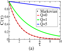
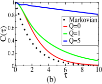
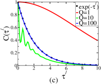
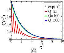
Figure 1: Decay of entanglement as measured by concurrence $C(t)$ with time at different values of the parameter $Q$ and $R$. Here we have used $\theta=\pi/2$. Plots for different $Q$ values at (a) $R=100$ (b) $R=1$ (c) $R=0.01$ and (d) $R=0.001$. Plots (a) and (b) are in units of Markovian decay rate $\Gamma_{M}$, i.e $\tau=\Gamma_{M}t$, while plots (c) and (d) are in units of rescaled decay rate $\frac{\Gamma_{M}}{Q^{2}}$ i.e $\tau^{\prime}=\frac{\Gamma_{M}}{Q^{2}}t$

.

Next we analyze the Markovian and non-Markovian regimes of the dynamics, for that we define the following parameters: $\tau=\Gamma_{M}t,~{}~{}~{}Q=\frac{J}{\lambda},~{}~{}R=\frac{\lambda}{\Gamma_{M}}$. Therefore, using this parametrization we have

$$\Gamma_{+}(t) = \frac{\tau}{2[1+9Q^{2}]}-\frac{[1-9Q^{2}][1-e^{-R\tau}\cos(3QR\tau)]}{2R[1+9Q^{2}]^{2}}$$ (31)

$$-\frac{3Q}{R[1+9Q^{2}]^{2}}e^{-R\tau}\sin(3QR\tau)$$

$$\Gamma_{-}(t) = \frac{\tau}{2[1+Q^{2}]}-\frac{[1-Q^{2}][1-e^{-R\tau}\cos(QR\tau)]}{2R[1+Q^{2}]^{2}}$$ (32)

$$-\frac{Q}{R[1+Q^{2}]^{2}}e^{-R\tau}\sin(QR\tau).$$

In order to understand how the Markovian limit is obtained from the above expressions, we plot in Fig. 1(a)-(b) $\mathcal{C}(\tau)$ for $\theta=\pi/2$ with respect to dimensionless parameter $\tau$ for $R=100$ and $R=1$ at different values of $Q$. We observe that the Markovian curve is recovered for $R>>1$ with $Q=0$. We can understand this behaviour of $\mathcal{C}(t)$ by looking at the different paramters involved. The typical time scale over which the system of two qubits changes is $\tau_{s}\sim 1/J$ and the time scale over which the bath changes is $\tau_{B}\sim 1/\lambda$ while relaxation time scale for each qubit would be given by $\tau_{R}\sim 1/\Gamma_{M}$. It means $R>>1$ implies $\tau_{B}<<\tau_{R}$ and $Q<1$ implies $\tau_{R}<\tau_{s}$. Thus physically $R>>1$ and $Q<1$ would imply that the system evolves over a large time compared to very fast bath dynamics. Therefore Markovian regime corresponds to $R>>1$ and $Q<1$ and we have

$$\Gamma_{+}(t)=\Gamma_{-}(t)=\frac{\tau}{2}$$ (33)

and therefore we get standard Markovian limit:

$$\mathcal{C}(t)=\mathcal{C}(0)e^{-\frac{1}{2}\Gamma_{M}t}.$$ (34)

We observe that under the Markovian limit an initially unentangled state remains unentangled always. In situations where the spectral width $\lambda$ of the bath is narrower than the energy scale $J$ involved for the system implying $Q>>1$. This would mean $\tau_{R}<<\tau_{s}$. In Fig. 1(b), we observe for $R=1$ that as $Q$ increases from 0, there is larger devaition from the Markovian dynamics of the concurrence $\mathcal{C}(t)$. The general trend is similar for all values of $R$ as can be seen on comparison to Fig. 1(a). These observations suggest Markovian regime is in fact opposite to the regime $R<1$ and $Q>>1$, which we call as non-Markovian regime. The term that is responsible for this larger deviation can be attributed to first terms of $\Gamma_{-}(t)$ and $\Gamma_{+}(t)$ containing $Q^{2}$ in the denominator. For $Q^{2}>>1$ suggest defining another time scale

$$\tau^{\prime}=\frac{\Gamma_{M}}{Q^{2}}t.$$ (35)

The decay of entanglement defined by $\mathcal{C}(t)$ at various values of $Q$ for non-Markovian regime $R<1$ in terms of rescaled time $\tau^{\prime}=\tau/Q^{2}$ is shown in the Fig.1(c)-(d). We see that for large $Q$ the concurrence $\mathcal{C}(\tau^{\prime})$ coincides with exponential decay in units of the rescaled time. Next we see that before reaching the limiting behavior of exponential decay in rescaled time (35), we observe some oscillatory behavior Figure 1(c)-(d). The deviation from an exponential decay can be attributed to the memory effects developed in the two qubit system. This occurs clearly due to the second terms in $\Gamma_{-}(t)$ and $\Gamma_{+}(t)$. For $Q\gg 1$ we may approximate this as

$$\Gamma_{-}(\tau^{\prime}) \approx \frac{1}{2}\left[\tau^{\prime}+\frac{1-e^{-RQ^{2}\tau^{\prime}}\cos(RQ^{3}\tau^{\prime})}{RQ^{2}}\right]$$ (36)

$$\Gamma_{+}(\tau^{\prime}) \approx \frac{1}{18}\left[\tau^{\prime}+\frac{1-e^{-RQ^{2}\tau^{\prime}}\cos(3RQ^{3}\tau^{\prime})}{RQ^{2}}\right].$$ (37)

In order for the oscillatory term to be visible, we require the exponential decay term in (36)-(37) to be not too fast giving $RQ^{2}<1$, but simultaneously the oscillation frequency should be faster than the overall decay envelope $RQ^{3}>RQ^{2}>1$. The strongest oscillations therefore occur when $RQ^{2}\sim 1$, which agree with the numerical plots in Figure 1(c)-(d). The deviation from an exponential decay can be attributed to the memory effects developed initially, typical of non-Markovian behavior. The criterion for the strongest oscillatory behavior are satisfied when all the characteristic time scales are all approximately the same i.e $\tau_{R}\sim\tau_{s}\sim\tau_{B}$.

V Conclusions

In conclusion, we have derived a quantum master equation for system of two interacting qubits under the influence of local dissipation. Using the assumption that the correlation functions have the same form for each of the baths, the solution of master equation is found for the general $X$-type state. The time dependence of concurrence, a measure of entanglement is studied for a pure entangled state $|\Psi\rangle=\cos\frac{\theta}{2}|01\rangle+\sin\frac{\theta}{2}|10\rangle$ (a special case of $X$-type state) under both Markovian and non-Markovian regimes of the dynamics. It is found that for finite time evolution an unentangled state can go to an entangled state in contrast to the Markovian case where the unentangled state remains unentangled always. By identifying the parameter space, we have found that our results reduce to standard Markovian decay rate which in general is not a physically relevant regime self . In the physically relevant regime with narrower spectral width as compared to $J$, the decay rate is better approximated by $\Gamma(t)=\frac{\Gamma_{M}}{Q^{2}}$, which is the standard Markovian decay rate divided by the $Q^{2}$, which can be quite large in practice.

Next we compare our work with the several other works that studied non-Markovian dynamics of entanglement. Taking the example of Ref. RF2 , the authors derive the non-Markovian decay of the entanglement for the pure state $|\Psi\rangle=\cos\frac{\theta}{2}|01\rangle+\sin\frac{\theta}{2}|10\rangle$. The time dependence of concurrence is given by:

$$\mathcal{C}(t)={\rm max}\{0,C(0)G(t)\}$$ (38)

where

$$G(t)=e^{-\lambda t/2}\left[\cosh(\frac{\lambda t}{2}\delta)+\frac{1}{\delta}\sinh(\frac{\lambda t}{2}\delta)\right]$$ (39)

and $\delta=\sqrt{1-\frac{2\Gamma_{M}}{\lambda}}$ and $\Gamma_{M}$ is the Markovian decay rate. Our result Eqn. (30) is more general than above result. The results in these works RF1 ; RF2 ; RF3 ; RF4 do not tell about the amount of entanglement and its decay that would be present in an entangled state generated from dissipation. To see more clearly the behavior, let us examine this in two limiting cases

Weak coupling limit $\Gamma_{M}\ll\lambda$: This regime corresponds to a weak coupling regime or a very broad coupling to many frequency modes, which gives Markovian behavior. Here $\delta\approx 1-\frac{\Gamma_{M}}{\lambda}$ and the decay function $G(t)$ gives purely exponential behavior. To first order the decay function may be approximated as

$$G(t)\approx e^{-\Gamma_{M}t/2}$$ (40)

which is nothing but standard Markovian spontaneous decay.

Strong coupling limit $\Gamma_{M}\gg\lambda$: The reverse regime is when the linewidth of the bath is extremely narrow, which gives rise to strongly non-Markovian behavior. Here we may approximate $\delta=i\sqrt{\frac{2\Gamma_{M}}{\lambda}}$ and

$$G(t)=e^{-\lambda t/2}\left[\cos\left(\sqrt{\frac{\Gamma_{M}\lambda}{2}}t\right)+\sqrt{\frac{\lambda}{2\Gamma_{M}}}\sin\left(\sqrt{\frac{\Gamma_{M}\lambda}{2}}t\right)\right]$$

which corresponds to damped oscillations at frequency $\sqrt{\lambda\Gamma_{M}/2}$ and a decay envelope with rate $\lambda$. Thus we see that in both the cases the previous results do not yield the scaling factor $Q^{2}$ as derived in Eq. (35).

The current result would be important for applications where spontaneous emission is a serious drawback of using excited states, such as for quantum information processors, quantum simulators, and quantum metrological applications.

Appendix A

In this appendix we write the explicit forms of the various functions used in main text.

$$\eta(t) = \frac{\Gamma_{M}\lambda}{\lambda^{2}+J^{2}}\left[\lambda(1-e^{\lambda t}\cos Jt)+Je^{-\lambda t}\sin Jt\right]$$ (42)

$$\Sigma(t) = \frac{\gamma_{0}\lambda}{\lambda^{2}+9J^{2}}\left[\lambda(1-e^{\lambda t}\cos 3Jt)+3Je^{-\lambda t}\sin 3Jt\right]$$

$$\Gamma_{-}(t) = \frac{1}{2}\int_{0}^{t}\!\!dz~{}\eta(z)$$ (45)

$$= \frac{\Gamma_{M}\lambda}{2[\lambda^{2}+J^{2}]}\left[\lambda t-\frac{\lambda^{2}-J^{2}}{\lambda^{2}+J^{2}}[1-e^{-\lambda t}\cos Jt)]\right.$$

$$~{}~{}~{}~{}~{}~{}~{}~{}~{}~{}~{}~{}~{}~{}~{}~{}~{}~{}\left.-\frac{2\lambda J}{\lambda^{2}+J^{2}}e^{-\lambda t}\sin Jt\right]$$

$$\Gamma_{+}(t) = \frac{1}{2}\int_{0}^{t}\!\!dz~{}\Sigma(z)$$ (47)

$$= \frac{\Gamma_{M}\lambda}{2[\lambda^{2}+9J^{2}]}\left[\lambda t-\frac{\lambda^{2}-9J^{2}}{\lambda^{2}+9J^{2}}[1-e^{-\lambda t}\cos 3Jt)]\right.$$

$$~{}~{}~{}~{}~{}~{}~{}~{}~{}~{}~{}~{}~{}~{}~{}~{}~{}~{}\left.-\frac{6\lambda J}{\lambda^{2}+9J^{2}}e^{-\lambda t}\sin 3Jt\right]$$

$$S_{-}(t) = \frac{\Gamma_{M}\lambda}{2[\lambda^{2}+J^{2}]}\left[Jt+\frac{2J}{\lambda^{2}+J^{2}}[1-e^{-\lambda t}\cos Jt)]\right.$$ (48)

$$~{}~{}~{}~{}~{}~{}~{}~{}~{}~{}~{}~{}~{}~{}~{}~{}~{}~{}\left.+\frac{\lambda^{2}-J^{2}}{\lambda^{2}+J^{2}}e^{-\lambda t}\sin Jt\right]$$

$$S_{+}(t) = \frac{\Gamma_{M}\lambda}{2[\lambda^{2}+9J^{2}]}\left[3Jt+\frac{6J}{\lambda^{2}+9J^{2}}[1-e^{-\lambda t}\cos 3Jt)]\right.$$ (49)

$$~{}~{}~{}~{}~{}~{}~{}~{}~{}~{}~{}~{}~{}~{}~{}~{}~{}~{}\left.+\frac{\lambda^{2}-9J^{2}}{\lambda^{2}+9J^{2}}e^{-\lambda t}\sin 3Jt\right]$$

References

- (1) M. A. Nielsen and I. Chuang, Quantum Computation and Quantum Communication ( Cambridge University Press ) .
- (2) M. Schlosshauer, Rev. Mod. Phys. 76, 1267
- (3) W. H. Zurek, Rev. Mod. Phys. 75, 715(2003) .
- (4) J. T. Barreiro, P. Schindler , O. Gühne ,T. Monz , M. Chwalla , C. F. Roos , M. Hennrich and R. Blatt, Nature Phys. 6, 943 (2010).
- (5) S. Schneider and G. J. Milburn, Phys. Rev. A 57, 3748 (1998).
- (6) Q. A. Turchette, C. J. Myatt, B. E. King , C. A. Sackett, D. Kielpinski , W. M. Itano , C. Monroe and D. J. Wineland, Phys. Rev. A, 62, 053807 (2000).
- (7) C. J. Myatt, B. E. King , Q. A. Turchette, C. A. Sackett, D. Kielpinski , W. M. Itano , C. Monroe and D. J. Wineland Nature, 403, 269 (2000).
- (8) E. Knill , R. Laflamme and W. H. Zurek, Science 279, 342 (1998).
- (9) S. Diehl , A. Micheli, A. Kantian, B. Kraus, H. Buechler, P. Zoller, Nature Phys. 4, 878 (2008).
- (10) F.Verstraete, M. M.Wolf, and J. I.Cirac, Nat. Phys.5, 633 (2009).
- (11) H. Weimer , M. Müller , I. Lesanovsky , P. Zoller and H.P. Büchler, Nature Phys. 6, 382 (2010).
- (12) M. B. Plenio et al., Phys. Rev. A 59, 2468 (1999).
- (13) Beige et al., J. Mod. Opt. 47, 2583 (2000).
- (14) P. Horodecki, Phys. Rev. A 63, 022108 (2001).
- (15) H. P. Beuer and F. Petruccione, The Theory of Open Quantum systems (Oxford, New York: Oxford University Press)(2005).
- (16) R. Lo Franco, B. Bellomo, S. Maniscalco, and G. Compagno, Int. J. Mod. Phys. B 27, 1345053 (2013).
- (17) B. Bellomo, R. Lo Franco, and G. Compagno, Phys. Rev. Lett. 99, 160502 (2007).
- (18) B. Bellomo, R. Lo Franco, and G. Compagno, Phys. Rev. A 77, 032342 (2008).
- (19) K. M. Fonseca Romero and R. Lo Franco, Phys. Scr. 86, 065004 (2012).
- (20) M. Q. Lone, and T. Byrnes, Phys. Rev. A 92, 011401(R), (2015).
- (21) B. M. Terhal and G.Burkard, Phys. Rev. A 71, 012336 (2005).
- (22) M. Ban, J. Phys. A: Math. Gen. 39, 1927 (2006).
- (23) M. M. Wolf, J. Eisert, T. S. Cubitt, and J. I. Cirac, Phys. Rev. Lett. 101, 150402 (2008).
- (24) F. Pastawski, L. Clemente and J. I. Cirac, Phys. Rev. A 83, 012304 (2011).
- (25) P. Haikka and S. Maniscalco, Phys. Rev. A 81, 052103 (2010).
- (26) W. M. Zhang, P. Y. Lo, H. N. Xiong, M. W. Y. Tu, and F. Nori, Phys. Rev. Lett. 109, 170402 (2012).
- (27) M. A. Cirone, G. De. Chiara, G. M. Palma and A. Recati, New J. Phys. 11 103055 (2009).
- (28) H. J. Carmichael, Statistical Methods in Quantum Optics I (Berlin: Springer-Verlag) (2008).
- (29) H. P. Breuer, B. Kappler and F. Petruccione, Phys. Rev. A 59, 1633 (1999).
- (30) H. P. Breuer, B. Kappler and F. Petruccione , Ann. Phys. (NY) 291, 36 (2001).
- (31) M. Schröder , U. Kleinekathöfer and M. Schreiber, J. Chem. Phys. 124 084903 (2006).
- (32) E. Ferraro ,M. Scala, R. Migliore and A. Napoli, Phys. Rev. A 80, 042112 (2009).
- (33) T. Yu and J. H. Eberly, Quantum Inf. Comput. 7, 459 (2007)
- (34) W.K.Wooters, Phys. Rev.Lett. 80, 2245 (1998).