Valley Hall effect in disordered monolayer MoS₂ from first principles

Abstract

Electrons in certain two-dimensional crystals possess a pseudospin degree of freedom associated with the existence of two inequivalent valleys in the Brillouin zone. If, as in monolayer MoS₂, inversion symmetry is broken and time-reversal symmetry is present, equal and opposite amounts of $k$-space Berry curvature accumulate in each of the two valleys. This is conveniently quantified by the integral of the Berry curvature over a single valley - the valley Hall conductivity. We generalize this definition to include contributions from disorder described with the supercell approach, by mapping (”unfolding”) the Berry curvature from the folded Brillouin zone of the disordered supercell onto the normal Brillouin zone of the pristine crystal, and then averaging over several realizations of disorder. We use this scheme to study from first-principles the effect of sulfur vacancies on the valley Hall conductivity of monolayer MoS₂. In dirty samples the intrinsic valley Hall conductivity receives gating-dependent corrections that are only weakly dependent on the impurity concentration, consistent with side-jump scattering and the unfolded Berry curvature can be interpreted as a $k$-space resolved side-jump. At low impurity concentrations skew scattering dominates, leading to a divergent valley Hall conductivity in the clean limit. The implications for the recently-observed photoinduced anomalous Hall effect are discussed.

I Introduction

Monolayers of MoS₂ and related transition-metal dichalcogenides (TMDs) have recently become the subject of intense investigation, due in part to the possibility of manipulating the so-called “valley” degree of freedom.xu-natphys14 These materials have the symmetry of a honeycomb structure with a staggered sublattice, thus lacking an inversion center. The bandstructure exhibits a direct gap at the two inequivalent valleys centered at the high-symmetry points $K$ and $K^{\prime}=-K$ in the Brillouin zone (see Fig. 1), where the topmost valence bands are are primarily composed of transition-metal $d$ states.mak_photo Time-reversal symmetry, which takes $\mathbf{k}$ into $-\mathbf{k}$ and therefore maps one valley onto the other, dictates that states in a given band at $K$ and $K^{\prime}$ carry antiparallel angular momenta. This inspired Xiao et al. to propose using circularly-polarized light as a means of selectively exciting carriers from a particular valley.xiao_graph ; xiao_valley The effect was rapidly confirmed experimentally, by demonstrating that excitation with circularly-polarized light results in polarized fluorescence.zeng ; mak_optical_valley ; cao

The broken inversion symmetry in monolayer MoS₂ induces a nonzero Berry curvature on the Bloch bands (in contrast, the Berry curvature vanishes identically for bilayer and bulk MoS₂, both of which are centrosymmetric). The Berry curvature is defined in terms of the cell-periodic Bloch states as

$$\Omega_{n,xy}({\mathbf{k}})=-2\text{Im}\sum_{n}\,\langle\partial_{k_{x}}u_{n{\mathbf{k}}}|\partial_{k_{y}}u_{n{\mathbf{k}}}\rangle\,,$$ (1)

and it modifies the current response to an applied electric field by adding an “anomalous velocity” term to the semiclassical equations of motion.xiao-rmp10 A well-known consequence is the anomalous Hall effect (AHE) in magnetic materials, where the Berry curvature is induced by broken time-reversal symmetry. The intrinsic, part of the anomalous Hall conductivity (AHC) is given by the Brillouin zone (BZ) integral of the Berry curvature summed over the occupied states,xiao-rmp10 ; nagaosa_review

$$\Omega_{xy}({\bf k}) = \sum_{n}\,f_{n{\bf k}}\Omega_{n,xy}({\bf k})$$ (2)

$$\sigma_{xy}^{0} = -\frac{e^{2}}{h}\int_{\rm BZ}\,\frac{d^{d}k}{(2\pi)^{d-1}}\Omega_{xy}({\bf k})\,,$$ (3)

where $f_{n{\bf k}}$ is the occupation factor and $d$ is the dimensionality. Here, the superscript 0 denoted that it is the intrinsic part of the AHC. For $d=2$ the AHC has units of conductance (S), and for $d=3$ it has units of conductivity (S/cm). The broken inversion symmetry in monolayer MoS₂ induces a nonzero Berry curvature on the Bloch bands (in contrast, the Berry curvature vanishes identically for bilayer and bulk MoS₂, both of which are centrosymmetric). The Berry curvature is defined in terms of the cell-periodic Bloch states as Monolayer MoS₂  is nonmagnetic, and the presence of time-reversal symmetry implies the relationxiao-rmp10

$$\Omega_{xy}(-\mathbf{k})=-\Omega_{xy}(\mathbf{k})\,.$$ (4)

Thus, equal and opposite amounts of Berry curvature accumulate in the two valleys, resulting in a cancellation of the valley Hall currents and a vanishing AHC. Time-reversal symmetry can however be broken by illuminating the sample with circularly-polarized light, leading to a photoinduced AHE. The valley-selective photoexcitation creates a carrier imbalance which in turn removes the exact cancellation between the Hall currents in the two valleys. This so-called valley Hall effect was first discussed for graphene systems with broken inversion symmetry,xiao_graph and later for monolayer MoS₂.xiao_valley The effect was subsequently measured by Mak at al. in transistors of MoS₂ monolayers.mak_valley

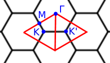
Figure 1: (Color online). Brillouin zone of monolayer MoS₂, partitioned into two triangular valleys delimited by lines of vanishing Berry curvature, drawn in red. The two valleys are centered at the high-symmetry points $K$ and $K^{\prime}$.

Compared to the conventional AHE in ferromagnetic metals, the theoretical modeling of the photoinduced AHE in TMDs poses the additional challenge that the AHC should in principle be calculated for a nonequilibrium photoexcited state, but to our knowledge, such a calculation has not yet been attempted. Instead, an approximate but more tractable approach is often used.xiao_graph ; xiao_valley ; mak_valley The idea is to introduce an auxiliary quantity $\sigma_{xy}^{V}$, which we will call the valley Hall conductivity (VHC), defined as the integral of the Berry curvature over a single valley domain in the BZ. For example, the intrinsic VHC of the valley centered at $K$ in Fig. 1 is

$$\sigma_{xy}^{0,K}(\varepsilon_{F})=-\frac{e^{2}}{h}\int_{K}\frac{d^{2}k}{2\pi}\Omega_{xy}(\mathbf{k})\,.$$ (5)

and similarly for the valley centered at $K^{\prime}$. (The demarcation of the two valley domains will be discussed further in Sec. II.1. Equation (5) depends on the Fermi level $\varepsilon_{F}$ through the occupation factors in Eq. (2).) The photoinduced AHC $\sigma_{xy}$ is then approximated by the sum of the VHCs in the two valleys, positing a Fermi-level shift $\delta\varepsilon$ between them to mimic the effect of the valley-selective photoexcitation,

$$\delta\sigma_{xy}(\varepsilon_{F},\delta\varepsilon)=\sigma_{xy}^{K}(\varepsilon_{F}+\delta\varepsilon)+\sigma_{xy}^{K^{\prime}}(\varepsilon_{F})\,.$$ (6)

When $\delta\varepsilon=0$ the AHC vanishes, and a nonzero $\delta\sigma_{xy}$ appears when $\delta\varepsilon\not=0$. This approach, also allows for a direct comparison with model calculations without considering the details of how the carrier imbalance between valleys is generated.

This will be the basic approach taken in the present work. We have suppressed the superscript 0 from this last equation to emphasize that it remains valid when the non-intrinsic contributions which we will now discuss are taken into account.

Impurities are always present in real samples, and their extrinsic contributions to the photoinduced AHE in TMDs should be taken into account alongside the intrinsic response described by Eqs. (5) and (6). This is well known in the context of the AHE in ferromagnetic metals, where historically two types of extrinsic contributions have been considered - side jump and skew scattering.nagaosa_review In a simplified picture, the side-jump effect originates in the anomalous velocity that a wave packet may acquire as it moves through an impurity potential, while skew scattering arises from the chiral part of a standard transition-rate expression. With some effort, both contributions can be incorporated into the semiclassical Boltzmann-transport framework.sinitsyn_coordinate

The correspondence between the semiclassical treatment of the AHC and a fully quantum-mechanical (Kubo-Streda) calculation based on a perturbative expansion in powers of the disorder strength was carefully worked out in Ref. sinitsyn_link, . It became clear from that analysis that not all terms fall distinctly into either of the above physical interpretations of extrinsic contributions to the AHC, and for many purposes it is more practical to base the distinction on the scaling with impurity concentration.nagaosa_review According to this viewpoint skew-scattering is defined as the part of the AHC which scales inversely with the impurity concentration, while the part which is independent of the impurity concentration has both intrinsic and side-jump components. Although the intrinsic contribution is sharply defined theoretically in terms of the electronic structure of the pristine crystal by Eq. (3), experimentally it is not known how to separate it from the side-jump part. Note that the anomalous Hall response of pristine samples at low temperatures is dominated by skew-scattering, with the intrinsic contribution only becoming significant in moderately resistive samples (where it competes with side-jump scattering). This analysis, originally developed for the AHC in ferromagnetic metals, carries over to the VHC and photoinduced AHC in TMDs.

It is well established that sulfur vacancies constitute the main source of disorder in MoS₂.zhou_defects ; liu_defects ; ma_defects ; zhou_defects1 ; wei_defects ; asl_defects The formation energies and thermodynamics of these defects have been thoroughly studied,komsa but their influence on transport and optical properties remains largely unexplored. Modeling the effects of disorder from first-principles is a challenging task in general, but there are noteworthy examples where the AHC in ferromagnetic materials has been calculated using the coherent potential approximation;velicky ; faulkner ; butler ; ebert ; blugel_skew ; kudr also, an ab initio implementation of the side-jump contribution to the AHC has been carried out assuming scattering centers with delta-function potentials.jurgen

In this work, we develop a computational scheme that allows us to include in a realistic manner the effect of impurities in the calculation of the VHC and of the photoinduced AHE in TMDs. In a first step, we perform several supercell calculations at the desired impurity concentration, corresponding to different realizations of disorder. In order to carry out the calculations efficiently while maintaining first-principles-like accuracy, we construct effective Hamiltonians in a Wannier-function basis, starting from density functional theory calculations on smaller cells.berlijn_effective Recall that the definition of the VHC in Eq. (5) requires identifying the individual valley domains in the BZ where the Berry curvature is to be integrated. It is not clear a priori how to do so in the context of a supercell calculation, since the electronic states cannot be labeled by wavevectors in the normal BZ of Fig. 1. In order to overcome this difficulty, in a second step we use a “BZ unfolding” techniqueku_unfolding to map the results of the supercell calculation onto the normal BZ of the pristine crystal. More precisely, we express the AHC of each disordered supercell configuration as an integral of the supercell Berry curvature over the folded BZ, and then unfold the Berry curvature onto the normal BZ according to the prescription of Ref. bianco_unfolding, . Having done that, the VHC (including the contributions from disorder) can then be obtained by integrating the unfolded Berry curvature over a single valley domain in Fig. 1, and averaging the result over several realizations of disorder.

We have used the above first-principles-based methodology to study the influence of sulfur vacancies on the VHC of MoS₂as well as the photoinduced AHC, which is the quantity measured in experiments. The calculated VHC as a function of defect concentration was compared with model calculations where the valence and conduction-band edges in each valley are described by a massive Dirac Hamiltonian with a random distribution of delta-function scatterers.sinitsyn_link

The paper is organized as follows. We start Sec. II by reviewing some basic features of the electronic structure of MoS₂. We then evaluate the intrinsic VHC [Eq. (5)] and photoinduced AHC [Eq. (6)] for the massive Dirac Hamiltonian without disorder, and carry out the corresponding ab initio calculations for pristine MoS₂. Our main results are presented in Sec. III, where disorder effects are included in the calculation of the VHC, both for the massive Dirac Hamiltonian and for MoS₂  with sulfur vacancies. The two types of calculations are found to be in reasonable agreement, and we then proceed to calculate the photoinduced AHC for the disordered massive Dirac model as a function of gating voltage and Fermi-level shift, finding good agreement with the experimental measurements. Our conclusions are summarized in Sec. IV, and the appendices present the details of the ab initio calculations, the BZ unfolding method, and the effective-Hamiltonian methodology.

II Pristine MoS₂

II.1 Energy bands and Berry curvature

Ab initio density-functional theory calculations were carried out for monolayer MoS₂  as described in Appendix A.1. The calculated Kohn-Sham energy bands are shown in the upper panel of Fig. 2, color-coded by the spin component $\langle S_{z}\rangle$ orthogonal to the layer. The minimum direct gap is situated at $K$ and $K^{\prime}=-K$, with a value of $\sim 1.7$ eV. Away from the time-reversal-invariant points $\Gamma$ and ${\rm M}$ the spin degeneracy is split by the combination of broken inversion symmetry and spin-orbit coupling (the degeneracy is actually protected along the entire $\Gamma$-${\rm M}$ line by mirror symmetry). The two topmost valence bands exhibit a maximum spin-orbit splitting of $\sim 0.15$ eV at $K$ and $K^{\prime}$, where $S_{z}$ is a good quantum number and Kramers-degenerate partners have opposite spin character: $\varepsilon_{K\uparrow}=\varepsilon_{K^{\prime}\downarrow}$.

The lower panel of Fig. 2 shows the Berry curvature summed over the valence bands, Eq. (2). In agreement with Eq. (4), $\Omega_{xy}$ is an odd function of ${\mathbf{k}}$. Its magnitude peaks at the minimum-gap points $K$ and $K^{\prime}$, where the sign is dictated by the dominant contributions coming from the topmost valence bands. At $K$ those bands are mainly composed of molybdenum $d$-states with $m_{l}=2$; according to the optical selection rulescao those states can be excited with left-handed polarized light. The Berry curvature has a secondary peak between $\Gamma$ and $K$; there, a pair of lower-lying valence bands approaches the topmost ones, and also contributes significantly to the Berry curvature.

It should be noted that because the Berry curvature is induced by the broken spatial inversion, it is not directly related to the spin-orbit splitting evident in Fig. 2; in fact, $\Omega_{xy}$ is practically unaltered if the spin-orbit interaction is switched off. (This is in sharp contrast to the Berry curvature induced by broken time-reversal symmetry in ferromagnetic metals, which vanishes in the absence of spin-orbit coupling.xiao-rmp10 ; nagaosa_review ) Likewise, the extrinsic scattering contributions do not rely on spin-orbit coupling. Thus one can use a spinless model such as the massive Dirac Hamiltonian of Sec. II.2.1 to describe the band edges and valley Berry curvature in MoS₂; spin is then accounted for by inserting a factor of two in the calculated $\Omega_{xy}$.

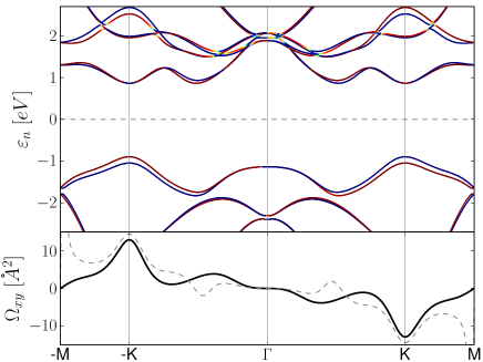
Figure 2: (Color online). Top: Calculated bandstructure of monolayer MoS₂. Energies are measured from the Fermi level, and the bands are color-coded by the spin expectation value $\langle S_{z}\rangle$, with red corresponding to spin up and blue to spin down. Bottom: Berry curvature summed over the valence bands [Eq. (2)]. The dashed line is the Berry curvature evaluated from the two topmost valence bands.

The Hamiltonian of monolayer MoS₂ is invariant under reflection across the vertical planes containing the lines that connect a Mo atom to the neighboring S atoms. The corresponding symmetry elements in reciprocal space are the $\Gamma$-${\rm M}$ mirror lines. The Berry curvature transforms like a magnetic field in reciprocal space.xiao-rmp10 In particular, the component $\Omega_{xy}=\Omega_{z}$ is odd under reflection across the $\Gamma$-${\rm M}$ lines, and hence it vanishes along those lines, which form the boundaries between the two valleys in Fig. 1. This allows us to uniquely define the intrinsic VHC according to Eq. (5).

II.2 Intrinsic Valley Hall conductivity

II.2.1 Massive Dirac model

The valence and conduction-band edges of a single valley of MoS₂ and related materials are often modeled by the massive Dirac Hamiltonian.xu-natphys14 ; xiao_graph ; xiao_valley The Hamiltonian for the $K$ valley in Fig. 2 reads

$$H({\mathbf{k}})=\hbar v(-k_{x}\sigma_{x}+k_{y}\sigma_{y})+\Delta\sigma_{z}\,,$$ (7)

where ${\mathbf{k}}=(k_{x},k_{y})$ is measured from the valley center $K$, $\sigma_{i}$ are the Pauli matrices, and $\Delta$ is the mass parameter. The energy eigenvalues and Berry curvature are

$$\varepsilon_{\pm}({\mathbf{k}}) = \pm\sqrt{\Delta^{2}+v^{2}\hbar^{2}k^{2}}$$ (8)

$$\Omega_{\pm,xy}({\mathbf{k}}) = \pm\frac{\Delta v^{2}\hbar^{2}}{2(\Delta^{2}+v^{2}\hbar^{2}k^{2})^{3/2}}\,,$$ (9)

where $k^{2}=k_{x}^{2}+k_{y}^{2}$. In the case of the $K^{\prime}$ valley Eq. (8) remains unchanged, while Eq. (9) flips sign.

If the Fermi level lies in the conduction band ($\varepsilon_{F}>\Delta$), the VHC becomes

$$\sigma_{xy}^{0,K} =-\frac{2e^{2}}{h}\bigg{[}\int\frac{d^{2}k}{2\pi}\Omega_{-}(k)+\int_{|k|<k_{F}}\frac{d^{2}k}{2\pi}\Omega_{+}(k)\bigg{]}$$

$$=\frac{e^{2}}{2h}-\frac{e^{2}\Delta}{2h}\Big{(}\frac{1}{\Delta}-\frac{1}{\varepsilon_{F}}\Big{)}.$$ (10)

The valley and spin degrees of freedom can be included by coupling four copies of this model corresponding to spin and valley degrees of freedom. Referring to the band structure of MoS₂ we find that in the vicinity of the valleys the massive Dirac model provides a good fit if we take $\Delta=0.86$ eV. The velocity $v$ is calculated as $v^{2}=\Delta/m^{*}_{e}$, where $m^{*}_{e}=0.4m_{e}$ is the effective mass of the conduction band valley.

For the ungated case where $\varepsilon_{F}$ is in the gap, the model gives an intrinsic VHC of $e^{2}/2h$. The deviation from that result measures the contribution from lower lying valence bands and the crystal potential, which gives rise to non-hyperbolic bands away from the top of the valleys. It should be noted though, that a Chern insulating system with an inversion center will retain the exact value $\sigma_{xy}^{0,K}=e^{2}/2h$ when the crystal potential is included, because symmetry implies $\Omega({\mathbf{k}})=\Omega(-{\mathbf{k}})$ and the topology implies $\sigma_{xy}^{0}=2\sigma_{xy}^{0,K}=e^{2}/h$.haldane ; kane_review For MoS₂ we find $\sigma_{xy}^{0,K}=0.71e^{2}/h$ and since each spin channel contributes an equal amount of curvature, this corresponds to 71% of the result for the massive Dirac Hamiltonian.

As discussed in the introduction, measuring the valley Hall effect requires generating a carrier imbalance between the two valleys. Since experimental realizations usually involves a gate, we include an overall Fermi level $\varepsilon_{F}$ such that the Fermi level in one valley is $\varepsilon_{F}$ and in the other valley it is $\varepsilon_{F}+\delta\varepsilon$ due to the presence of polarized light. If we assume left-handed polarized light, we can then calculate the photoinduced AHC as a function of $\delta\varepsilon$ in the $K$ valley, which will depend on the strength of the optical perturbation in an experimental setup. Combining Eqs. (6) and (II.2.1) we obtain for $\varepsilon_{F}>\Delta$,

$$\delta\sigma_{xy}^{0}(\varepsilon_{F},\delta\varepsilon)=-\frac{e^{2}\Delta}{2h}\Big{(}\frac{1}{\varepsilon_{F}}-\frac{1}{\varepsilon_{F}+\delta\varepsilon}\Big{)}\,.$$ (11)

We can also express this quantity in terms of carrier imbalance $\delta n_{c}$ between the conduction-band edges in the two valleys. For a single valley

$$n_{c}(\varepsilon_{F})=\frac{\pi k_{F}^{2}}{(2\pi)^{2}}=\frac{\varepsilon_{F}^{2}-\Delta^{2}}{4\pi v^{2}\hbar^{2}},$$ (12)

so that

$$\delta n_{c}=\frac{2\varepsilon_{F}\delta\varepsilon+\delta\varepsilon^{2}}{4\pi v^{2}\hbar^{2}}.$$ (13)

For $\delta\varepsilon\ll\varepsilon_{F}$ we then get

$$\delta\sigma_{xy}^{0}\approx-\frac{e^{2}}{h}\frac{\Delta}{\varepsilon_{F}^{2}}\delta\varepsilon\approx-\frac{2\pi e^{2}v^{2}\hbar\Delta}{\varepsilon_{F}^{3}}\delta n_{c}.$$ (14)

Thus, in this limit the photoinduced AHC becomes linear in both the small energy shift $\delta\varepsilon$ and in the small carrier imbalance $\delta n_{c}$. An expression similar to this one was derived in Ref. mak_valley, , but with the Fermi level in the gap. That expression can be obtained by setting $\varepsilon_{F}=\Delta$ in Eq. (14). As will be shown in Sec. III.5, the position of the Fermi level is minuscule for the intrinsic as well as the sidejump contributions, but can have a large effect on the skew scattering contribution, which becomes dominant for clean samples.

II.2.2 First-principles calculations

In Fig. 3 we show the intrinsic photoinduced AHC $\delta\sigma_{xy}^{0}$ from a single spin channel as a function of the single-valley energy shift $\delta\varepsilon$, for $\varepsilon_{F}=0$. It should be noted that due to the spin-orbit split valence bands in MoS₂, it is possible to selectively excite a single spin channel by using an optical frequency tuned to the transition between the topmost valence band and the conduction band.xiao_valley ; mak_valley The ab initio calculations are seen to agree very well with the model results at the bottom of the valley. When the energy shift approaches $\sim 0.1$ eV the secondary valley located between $\Gamma$ and $K$ starts to contribute, and the model results become unreliable.

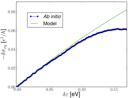
Figure 3: (Color online). Intrinsic photoinduced anomalous Hall conductivity of a single layer of MoS₂ without gating ($\varepsilon_{F}=0$), plotted as a function of the Fermi-level shift $\delta\varepsilon$ in the $K$ valley. The thin green line corresponds to Eq. (14) for the massive Dirac model with the parameters given in the text, and the blue dotted line was obtained by evaluating Eqs. (5) and (6) from first-principles.

The measurements of the valley Hall effect reported in Ref. mak_valley, involved photoexcitation of states in a single valley. In that work, the carrier density was estimated from photoconductivity measurements, and the photoinduced AHC was displayed as a function of carrier density. The typical density of photoexcited carriers reported in Ref. mak_valley, is of the order of $10^{-11}$ cm^-2, which corresponds to an energy shift $\delta\varepsilon\sim 1$ meV; this is far below the point where the linear model (14) breaks down.

III Disordered MoS₂

Experimental as well as theoretical studies has recently demonstrated that sulfur vacancies are the dominant source of disorder in MoS₂.zhou_defects ; liu_defects ; ma_defects ; zhou_defects1 ; wei_defects ; asl_defects In the following we will thus exclusively focus on the sulfur vacancies and calculate how they affect the VHC. The results will be analyzed in terms of an impurity averaged unfolded Berry curvature, which will be defined below. However, before we delve into the ab initio calculations we will briefly review the theoretical results for the AHC in a massive Dirac model with impurity scattering.

III.1 Massive Dirac model

To obtain a model result for the VHC of disordered MoS₂, we use the extrinsic contribution to the AHC of the massive Dirac Hamiltonian (7), which has been calculated in the limit of weak and dilute scattering.sinitsyn_link The impurity potential for a given configuration is $V(\mathbf{r})=\sum_{i}V_{i}\delta(\mathbf{r}-\mathbf{R_{i}})$, where $\mathbf{R_{i}}$ are impurity sites. The result for the intrinsic (0), side jump (SJ) and skew scattering (SS) contributions to the VHC of the $K$ valley is then

$$\sigma^{0,K}_{xy}=\frac{e^{2}\Delta}{2h\sqrt{(v\hbar k_{F})^{2}+\Delta^{2}}},$$ (15)

$$\sigma^{SJ,K}_{xy}=\frac{e^{2}\Delta}{2h\sqrt{(v\hbar k_{F})^{2}+\Delta^{2}}}\bigg{[} \frac{4(v\hbar k_{F})^{2}}{4\Delta^{2}+(v\hbar k_{F})^{2}}$$ (16)

$$+\frac{3(v\hbar k_{F})^{4}}{(4\Delta^{2}+(v\hbar k_{F})^{2})^{2}}\bigg{]},$$

$$\sigma^{SS,K}_{xy}=\frac{e^{2}\langle V_{i}^{3}\rangle_{c}\Delta}{hx\langle V_{i}^{2}\rangle_{c}^{2}}\frac{(v\hbar k_{F})^{4}}{(4\Delta^{2}+(v\hbar k_{F})^{2})^{2}}.$$ (17)

Equation (15) is just Eq. (II.2.1) recast in a different form. As mentioned in the Introduction, scattering contributions which are independent of the impurity concentration $x$ are classified as side-jump, and those which scale inversely with $x$ are classified as skew-scattering. In particular, the second term in Eq. (16) originates from a fourth-order expansion of the scattering rate, and could thus be regarded as a skew-scattering contribution. Furthermore, the side-jump contribution contains contributions that cannot directly by ascribed to a coordinate shift.sinitsyn_link

In Fig. 4 we show the VHC as a function of impurity concentration at different Fermi level shifts calculated within the model with $\Delta=0.86$ eV and $\langle V_{i}^{3}\rangle_{c}/\langle V_{i}^{2}\rangle_{c}^{2}=-0.4$ eV^-1. The VHC converges to the side jump at large impurity concentrations, but one should keep in mind that the model results are derived under the assumption of dilute disorder and weak scattering. The side jump correction to the intrinsic part becomes larger for higher density of states at the Fermi level and is neglectable at very low carrier concentrations. Furthermore, at low carrier concentrations, the skew scattering only becomes significant at very low impurity concentrations. It thus appears that for low carrier concentrations, the intrinsic contribution gives a good account of the AHC - even at rather low impurity concentrations.

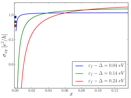
Figure 4: (Color online). Valley Hall conductivity of the disordered massive Dirac model, Eqs. (15)-(17), evaluated as a function of impurity concentration $x$ for three different gating levels, with $\langle V_{i}^{3}\rangle_{c}/\langle V_{i}^{2}\rangle_{c}^{2}=-0.4$ eV and $\Delta=0.86$ eV. The squares at $x=0$ correspond to the intrinsic contribution of Eq. 15.

III.2 Unfolded band structure and Berry curvature

In pristine systems, the Berry curvature provides a useful $k$-resolved measure of the Hall conductivity. For example, from Fig. 2 it is clear that states near the valleys at $K$ and $K^{\prime}$ have the largest potential for contributing to the VHC. However, if we would like to know how a given distribution of impurities affects the VHC, this picture immediately breaks down since the pristine Brillouin zone is no longer relevant due to broken translational symmetry. On the other hand, if a given impurity distribution is represented in a supercell, the VHC will still be given as a $k$-space integral of the Berry curvature, but now the domain will be the Brillouin zone corresponding to the supercell (SBZ), which is not directly comparable to the normal Brillouin zone (NBZ). Nevertheless, we can expand the supercell states in terms of states in the pristine system and thus unfold the supercell curvature to the pristine Brillouin zone. For a general band quantity $a_{N}({\mathbf{K}})$ defined in SBZ we can thus define the unfolded quantity $a^{(u)}_{n}({\mathbf{k}})$ in the NBZ as

$$a^{(u)}_{n}({\mathbf{k}})=\sum_{N}|\langle N{\mathbf{K}}|n{\mathbf{k}}\rangle|^{2}a_{N}({\mathbf{K}}),$$ (18)

where ${\mathbf{K}}$ is the SBZ crystal momentum, which is related to $k$ by translation of a supercell reciprocal lattice vector. Brillouin zone integrals can be written in terms of the unfolded function since

$$A =\int_{\rm SBZ}d{\mathbf{K}}\sum_{N}a_{N}({\mathbf{K}})$$

$$=\int_{\rm SBZ}d{\mathbf{K}}\int_{\rm NBZ}d{\mathbf{k}}\sum_{nN}|\langle N{\mathbf{K}}|n{\mathbf{k}}\rangle|^{2}a_{N}({\mathbf{K}})$$

$$=\int_{\rm NBZ}d{\mathbf{k}}\sum_{n}a^{(u)}_{n}({\mathbf{k}})\,,$$ (19)

where a complete set of NBZ states were inserted in the second line and it was used that $\langle N{\mathbf{K}}|n{\mathbf{k}}\rangle$ is only non-vanishing if ${\mathbf{k}}$ downfolds to ${\mathbf{K}}$.

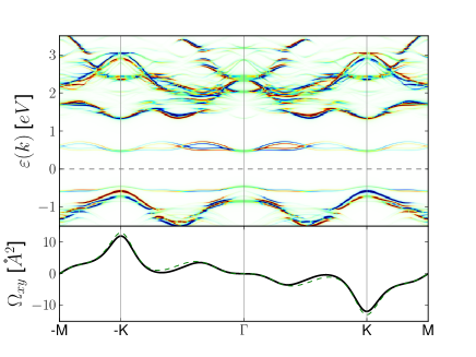
Figure 5: (Color online). Unfolded spectral function (top) and Berry curvature (bottom) of a $3\times 3$ MoS₂ supercell with a single sulfur vacancy. The Fermi level $\varepsilon_{F}=0$ is in the gap and the Berry curvature is largely unaffected by the presence of the impurity (the Berry curvature for pristine MoS₂ , taken from Fig. 2, is drawn as a dashed green line).

The method of unfolding $k$-space quantities has previously been applied to band structures of disordered systemsku_unfolding ; berlijn_effective and more recently to unfolding the Berry curvature.bianco_unfolding In the case of band structures the object of interest is the spectral function

$$A^{(u)}(\omega,{\mathbf{k}})=\sum_{nN}|\langle N{\mathbf{K}}|n{\mathbf{k}}\rangle|^{2}\delta(\omega-\varepsilon_{N{\mathbf{K}}}).$$ (20)

The Berry curvature is somewhat more complicated since, a naive application of Eq. (18) leading to

$$\Omega^{(u)}({\mathbf{k}})=\sum_{nN}|\langle N{\mathbf{K}}|n{\mathbf{k}}\rangle|^{2}f_{N{\mathbf{K}}}\Omega_{N}({\mathbf{K}}),$$ (21)

becomes gauge dependent. In Ref. bianco_unfolding, Eq. (21) it was shown h how to generalize Eq. (18) to obtain an explicitly gauge invariant quantity. In the present work we have applied the gauge invariant expression for all calculations.

III.3 Sampling impurity configurations

In Fig. 5 we show the unfolded spectral function and Berry curvature of a periodic structure obtained as $3\times 3$ MoS₂ unit cell with a single sulfur vacancy. The vacancy is seen to introduce both occupied and unoccupied states in the gap, but the Berry curvature is largely unaffected by such rather localized states. This system is a example of a $x=1/18=0.56$ impurity concentration, but is not necessarily representative of this disorder concentration in general. As it turns out the Berry curvature is largely insensitive to the impurity configuration as long as the Fermi level is in the gap. However, the situation changes dramatically when the Fermi level is shifted to the conduction band. This situation is shown in Fig. 6. The blurred features in the unfolded spectral function is associated with scattering states and are accompanied by spiky feature in the Berry curvatures. From the spectral representation of the Berry curvature Eq. (22), it is clear that such features arise whenever occupied and unoccupied states come close to the Fermi level.

In experiments with MoS₂ transistors the Fermi level is typically controlled with a gate voltage.mak_valley Furthermore, exfoliated MoS₂ usually exhibits an intrinsic $n$-doping, which is attributed to Re impurities.komsa For these reasons, we have chosen to pin the Fermi level to the conduction band in the following. This will facilitate the comparison with experiments as well as model calculations.

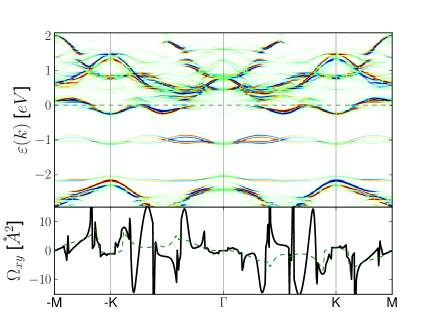
Figure 6: (Color online). Same as Fig. 5, except that the Fermi level has been shifted to the conduction band, where the impurities induce large modifications of the Berry curvature.

In order to perform a faithful calculation of the conductivity at a given impurity concentration, one then has to average over a large number of impurity configurations. Such a procedure requires a high number of simulations in large unit cells and is not feasible with standard ab initio methods. To proceed we construct an effective Hamiltonian based on ab initio DFT calculations and Wannier functions. Given an impurity concentration, we thus randomly generate an impurity configuration and construct the corresponding Hamiltonian as described in Appendix B. For a given vacancy concentration, we perform calculations for $\sim 1000$ systems with randomly drawn impurity configurations in a $6\times 12$ supercell. The smallest impurity concentration considered was $x=1/216$, where we needed a larger supercell of $12\times 18$. As a first check of the method, we calculate the optical conductivity of MoS₂ at various S vacancy concentrations. The results are shown in Fig. 7 and as expected the impurities simply introduce a broadening of the spectra. We should note that the Wannier functions used to construct the tight-binding Hamiltonian was obtained by disentangling bands up to 3.0 eV above the conduction band minimum and the present calculation is thus only expected to be reliable up to 3.0 eV above the pristine absorption edge.

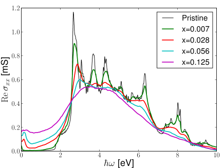
Figure 7: (Color online). Configuration-averaged optical absorption spectrum of MoS₂ at various impurity concentration.

III.4 Valley Hall conductivity

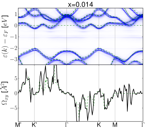
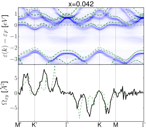
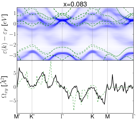
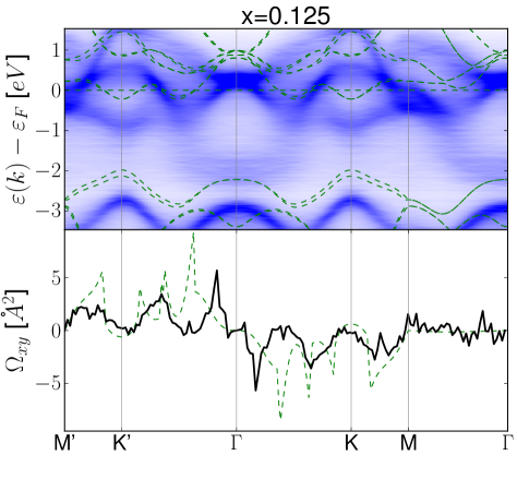
Figure 8: (Color online). Impurity averaged unfolded spectral function and Berry curvature of disordered MoS₂ with the Fermi level fixed in the conduction band. The dashed green lines shows the result for pristine MoS₂.

The lowest impurity concentration we have considered is $x=0.005$. Here the configurational averaged unfolded Berry curvature becomes very spiky and is not particularly informative. In Fig. 8 we show the configurational averaged unfolded Berry curvature for 4 different intermediate impurity configurations for $\varepsilon_{F}-\Delta=0.24$ and $\varepsilon_{F}-\Delta=0.24$. In general we observe that the peaks in the Berry curvature becomes enhanced and broadened, while the curvature retains its qualitative features. This tendency is maintained over a range of impurity concentrations ($x=0.02$ - $x=0.1$) and gives rise to a impurity independent increase in VHC. We will identify this with the side jump corrected VHC and the Berry curvatures in Fig. 8 thus comprises a measure of the $k$-space resolved side jump scattering. From the unfolded spectral function it is clear that the sulfur vacancies has the effect of lowering the overall potential, such that the conduction bands are lowered with respect to the fixed Fermi level at high impurity concentrations. However, for intermediate dopings the exact position of the Fermi level does not have a large effect on the VHC. In fact, raising the Fermi level with respect to the conduction band tends to lower the VHC, since more curvature from the conduction band will be included and this has the opposite sign of the dominating contribution from the valence bands. At larger impurity concentrations ($x=0.125$) the Berry curvature becomes more ”smeared” and will eventually average to zero. At this point the system is so strongly perturbed that it cannot be analyzed in terms of scattering events.

In Fig. 9 we show the VHC as a function of impurity concentration at different Fermi level shifts. At low impurity concentrations we observe a divergent behavior of the VHC. Comparing with Eqs. (15)-(16) we identify this with skew scattering processes. In terms of the unfolded curvature, this is the ”spiky” regime, where the averaged curvature largely looses the qualitative features of the pristine system. We note that as the impurity concentration $x$ is decreased, it becomes progressively harder to converge the results. This is due to the fact that the standard deviation for a given supercell size increases when $x$ becomes small, while at the same time we need very large supercells in order to perform calculations for small $x$.

At intermediate impurity concentrations the VHC reaches a flattened plateau, which we identify as the side jump regime. In this regime skew scattering is insignificant and the pristine result receives a small correction which is nearly independent of impurity concentration. Comparing with Fig. 4, we see that there is good qualitative agreement between the model and the ab initio results. A major difference is the fact that the ab initio VHC decreases at high impurity concentrations, whereas the model converges towards the side jump result. The reason is that the model results were derived under the assumption of dilute impurity concentration, and cannot be applied in this regime. Moreover, at large Fermi level shifts the deviations from the Dirac model begins to be important. In the present system the most important effect is the contribution from the secondary conduction band minimum between $\Gamma$ and $K$.

When the Fermi level comes close to the conduction band minimum, two crucial features can be observed from Figs. 4 and 9. First, the side jump correction becomes small such that the intrinsic VHC becomes a good estimate at intermediate impurity concentrations. Second, the critical impurity concentrations, where skew scattering starts to dominate, becomes rather small. For $\varepsilon_{F}-\varepsilon_{c}=0.04$ this concentration is $x\sim 0.005$ and will be even smaller when the Fermi level moves closer to the band edge.

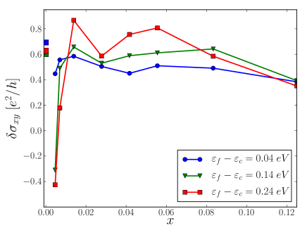
Figure 9: (Color online). Calculated VHC as a function of impurity concentration $x$. We show the result for three different positions of the Fermi level with respect to the conduction band minimum $\varepsilon_{c}$.

III.5 Photoinduced anomalous Hall conductivity

As mentioned previously, the experimentally measured quantity is the photoinduced AHC, which we express as the sum of the two VHCs. For small carrier imbalance this will be $\delta\sigma_{xy}(\varepsilon_{F},\delta\varepsilon)=d\sigma_{VH}(\varepsilon)/d\varepsilon|_{\varepsilon=\varepsilon_{F}}\delta\varepsilon$, where $\delta\varepsilon$ is the shift in Fermi level corresponding to the charge imbalance. A first principles evaluation of this expression including impurities is made difficult by the fluctuations involved in the configurational averaging procedure. However, the good agreement between the ab initio calculations of the VHC (Fig. 9) with the massive Dirac model (Fig. 4), suggests that we can obtain a reliable estimate of the photoinduced AHC from the Dirac model. For the skew scattering contribution we take $\langle V_{i}^{3}\rangle_{c}/\langle V_{i}^{2}\rangle_{c}^{2}=-0.4$ eV as in Fig. 4. Note that this value, and in particular the sign, is a non-trivial ab initio result obtained from the VHC calculations.

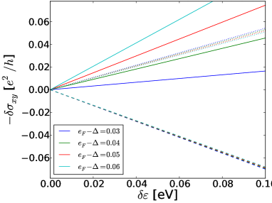
Figure 10: (Color online). Photoinduced AHC as a function of Fermi level shift $\delta\varepsilon$ between the valleys. States in the K valley are assumed excited corresponding to application of a left-handed polarized field. The dotted lines are the intrinsic $\delta\sigma^{0}_{xy}$, the dashed lines are $\delta\sigma^{0}_{xy}+\delta\sigma^{SJ}_{xy}$, and the solid lines are $\delta\sigma^{0}_{xy}+\delta\sigma^{SJ}_{xy}+\delta\sigma^{SS}_{xy}$. Note the large dependence on Fermi level when skew-scattering is included.

In Fig. 10 we show the photoinduced AHC calculated from Eqs. (15)-(17) with $x=0.01$. First of all it should be noted that the inclusion of side jump scattering gives a result, which is very close to the intrinsic contribution, except that the sign has been changed. This was already noted in Ref. mak_valley, For the VHC, the side jump only contributes a minor part to the scattering independent VHC. However, for the derivative, which is the relevant quantity for the photoinduced AHC, the side jump plays a dominant role. At small impurity concentrations, the skew scattering contribution will dominate. The skew scattering part of the VHC scales as $1/x$ and so does its contribution to the photoinduced AHC. Interestingly, the skew scattering contribution also has significant dependence on the position of the Fermi level and could explain the large dependence on gate voltage observed experimentally.mak_valley

IV Conclusions

A priori it is not clear that the intrinsic VHC provides a good descriptor for the VHC in a MoS₂ transistor setup, since the Hall conductivity is expected to diverge in the clean limit as a consequence of skew scattering.mak_valley Here we have used first principles calculations to investigate the effect of sulfur vacancies at different impurity concentrations. The influence of disorder was analyzed in $k$-space in terms of the unfolded Berry curvature and we have shown that the side jump regime appears as a concentration independent enhancement of the Berry curvature. The skew scattering introduces divergences in the Berry curvature and the unfolded Berry curvature becomes spiky and irrelevant. Nevertheless, we were able to converge the VHC calculations in the skew scattering regime, and recover the expected divergent behavior. The ab initio calculations show qualitative agreement with model calculations based on a massive Dirac Hamiltonian and allow us to extract a non-trivial value of the skew scattering potential $\langle V_{i}^{3}\rangle_{c}/\langle V_{i}^{2}\rangle_{c}^{2}=-0.4$ eV. The calculations allow us to estimate a critical impurity concentration $x$ where skew scattering starts to dominate. For $\varepsilon_{F}=40$ meV (with respect to the conduction band minimum) we find that $x\sim 0.005$ and below this point the intrinsic VHC becomes a poor descriptor.

A comparison with experimentsmak_valley indicates that indeed, the intrinsic VHC cannot be applied as a descriptor for the photoinduced valley Hall conductivity. As previously noted, the side jump contribution changes the sign of photoinduced AHC and we have shown that the skew scattering contribution is a likely explanation for the large gate dependence observed experimentally.mak_valley However, a reliable estimate of the skew scattering contribution requires knowledge of the impurity concentrations in the samples investigated, which is not presently available. It would be very interesting to perform measurements of the photoinduced AHC on MoS₂ samples with different impurity concentrations in order to unravel the roles played by side jump and skew scattering.

We have implicitly assumed a low temperature regime and therefore not discussed the effect of phonons. The effect of phonons on the longitudinal mobility in MoS₂ has been analyzed thoroughly,kristen but the influence on the transverse conductivity has so far not been considered. Furthermore, monolayer MoS₂ have been shown to exhibit strong excitonic effects huser_MoS2 ; louie_MoS2 due to poor screening in two-dimensional materials. The charge imbalance utilized in the experimental realization originates from optically generated electron-hole pairs, and if the Fermi level is close to the conduction band edge these effects could potentially severely limit the carrier mobility. We will leave these issues for future studies.

V Acknowledgement

This work was supported by the Danish Council for Independent Research, Sapere Aude Program, and by grants No. MAT2012-33720 from the Ministerio de Economía y Competitividad (Spain) and No. CIG-303602 from the European Commission.

Appendix A Calculational details

The calculations in the present work was performed with the tight binding method using parameters obtained from ab initio density functional calculations and projected Wannier functions.

A.1 Ab initio calculations and construction of Wannier orbitals

The ab initio density functional theory calculations were performed with the pwscf code from the Quantum Espresso package,quantum_espresso using the PBE functional. Norm-conserving pseudopotentials were used, and the calculations were carried out with a planewave cutoff of 100 Ry. The lattice parameter of MoS₂ was set to the experimental lattice constant of 3.16 Å, and 12 Å was used to separate the periodically-repeated images. All calculations were performed in a non-collinear spin framework, with fully relativistic pseudopotentials.

After converging the Kohn-Sham electronic structure, the valence and low-lying conduction Bloch bands were converted into projected Wannier functions using the Wannier90 code package.wannier90 For MoS₂ the projected Wannier orbitals were constructed using sulfur $p$ states and Mo $d$ states. The sulfur $s$ states were included in the ab initio calculations, but the low lying $s$-like Bloch bands were excluded from the wannierization. Unoccupied states were included by disentangling souza_disentangling bands up to 3.0 eV above the conduction band minimum. Finally the Wannier functions were used to construct the Kohn-Sham Hamiltonian in a tight-binding basis $H_{ij}(\mathbf{R})$, where $i,j$ denotes orbital indices within the unit cell and $\mathbf{R}$ is a lattice vector. The set of lattice vectors included were defined by the Wigner-Seitz cell corresponding to the applied ab initio $k$-point mesh. For example, in pristine MoS₂ with a $8\times 8$ $k$-point mesh, we have 22 orbitals (Mo $d$ and S $p$) and 64 lattice vectors (some of which are equivalent).

A.2 Tight-binding calculations

The majority of calculations in present work are tight-binding calculations with parameters obtained from a Wannier representation of the Kohn-Sham Hamiltonian $H_{ij}(\mathbf{R})$. In a tight-binding framework, the calculation of band structures from $H_{ij}(\mathbf{R})$ is of course equivalent to the standard Wannier interpolation.souza_disentangling At the sampled set of $k$-points, $H_{ij}(\mathbf{R})$ will thus yield the calculated Kohn-Sham eigenvalues and between the sampled points it smoothly interpolates. Similarly, a rigorous Wannier interpolation scheme can be constructed for the AHC,wang_ahc but this quantity cannot be calculated exactly in a bare tight-binding framework since the information contained in $H_{ij}(\mathbf{R})$ is not enough to evaluate the Berry curvature.

To see this explicitly we will briefly state the relevant expressions below. The starting point is the Berry curvature in its spectral representation where it can be written

$$\Omega_{\alpha\beta}(\mathbf{k}) =\sum_{m,n}(f_{n\mathbf{k}}-f_{m\mathbf{k}})$$ (22)

$$\times\frac{\langle u_{m\mathbf{k}}|\nabla_{\alpha}H(\mathbf{k})|u_{n\mathbf{k}}\rangle\langle u_{n\mathbf{k}}|\nabla_{\beta}H(\mathbf{k})|u_{m\mathbf{k}}\rangle}{(\varepsilon_{n\mathbf{k}}-\varepsilon_{m\mathbf{k}})^{2}},$$

with $\nabla_{\alpha}\equiv\partial/\partial k_{\alpha}$. We let $\varphi_{i}$ denote at set of localized orbitals and expand the Bloch states as

$$|\psi_{n\mathbf{k}}\rangle=\sum_{i}{C_{ni\mathbf{k}}}|\chi_{i\mathbf{k}}\rangle=\sum_{i\mathbf{R}}C_{ni\mathbf{k}}e^{i\mathbf{k}\cdot(\mathbf{R}+\mathbf{t}_{i})}|\varphi_{i\mathbf{R}}\rangle$$ (23)

where $\mathbf{t}_{i}=\langle\phi_{i\mathbf{0}}|\hat{\mathbf{r}}|\phi_{i\mathbf{0}}\rangle$. Note that the inclusion of $\mathbf{t}_{i}$ is purely a matter of convention. However, the present convention will prove highly convenient below. Matrix elements of the Bloch Hamiltonian and their gradients can now be written as

$$H_{ij\mathbf{k}}=\langle\chi_{i\mathbf{k}}|\hat{H}|\chi_{j\mathbf{k}}\rangle=\sum_{\mathbf{R}}e^{i\mathbf{k}\cdot(\mathbf{R}-\mathbf{t}_{i}+\mathbf{t}_{j})}H_{ij}(\mathbf{R}),$$ (24)

$$\nabla_{\mathbf{k}}H_{ij\mathbf{k}}=i\sum_{\mathbf{R}}(\mathbf{R}-\mathbf{t}_{i}+\mathbf{t}_{j})e^{i\mathbf{k}\cdot(\mathbf{R}-\mathbf{t}_{i}+\mathbf{t}_{j})}H_{ij}(\mathbf{R})$$ (25)

and in terms of these, the matrix elements appearing in Eq. (22) becomes

$$J_{\alpha mn}(\mathbf{k}) \equiv\langle u_{m\mathbf{k}}|\nabla_{\alpha}H(\mathbf{k})|u_{n\mathbf{k}}\rangle$$

$$=\sum_{ij\mathbf{R}}C^{*}_{mi\mathbf{k}}C_{nj\mathbf{k}}e^{i\mathbf{k}\cdot(\mathbf{R}-\mathbf{t}_{i}+\mathbf{t}_{j})}\langle\varphi_{i\mathbf{0}}|e^{i\mathbf{k}\cdot\hat{\mathbf{r}}}\nabla_{\alpha}H(\mathbf{k})e^{-i\mathbf{k}\cdot\hat{\mathbf{r}}}|\varphi_{j\mathbf{R}}\rangle$$

$$=-i\sum_{ij\mathbf{R}}C^{*}_{mi\mathbf{k}}C_{nj\mathbf{k}}e^{i\mathbf{k}\cdot(\mathbf{R}-\mathbf{t}_{i}+\mathbf{t}_{j})}\langle\varphi_{i\mathbf{0}}|[\hat{\mathbf{r}},\hat{H}]|\varphi_{j\mathbf{R}}\rangle$$

$$=-i\sum_{ijl\mathbf{R}\mathbf{R}^{\prime}}C^{*}_{mi\mathbf{k}}C_{nj\mathbf{k}}e^{i\mathbf{k}\cdot(\mathbf{R}-\mathbf{t}_{i}+\mathbf{t}_{j})}[\langle\varphi_{i\mathbf{0}}|\hat{\mathbf{r}}|\varphi_{l\mathbf{R}^{\prime}}\rangle\langle\varphi_{l\mathbf{R}^{\prime}}|\hat{H}|\varphi_{j\mathbf{R}}\rangle-\langle\varphi_{i\mathbf{0}}|\hat{H}|\varphi_{l\mathbf{R}^{\prime}}\rangle\langle\varphi_{l\mathbf{R}^{\prime}}|\hat{\mathbf{r}}|\varphi_{j\mathbf{R}}\rangle]$$

$$=-i\sum_{ijl\mathbf{R}\mathbf{R}^{\prime}}C^{*}_{mi\mathbf{k}}C_{nj\mathbf{k}}e^{i\mathbf{k}\cdot(\mathbf{R}+\mathbf{R}^{\prime}-\mathbf{t}_{i}+\mathbf{t}_{j})}[\mathbf{r}_{il\mathbf{R}^{\prime}}H_{lj\mathbf{R}}-H_{il\mathbf{R}^{\prime}}(\mathbf{r}_{lj\mathbf{R}}+\mathbf{R}^{\prime}\delta_{\mathbf{R}\mathbf{0}}\delta_{lj})]$$

$$=-i\sum_{ijl}C^{*}_{mi\mathbf{k}}C_{nj\mathbf{k}}[\mathbf{r}_{il\mathbf{k}}H_{lj\mathbf{k}}-H_{il\mathbf{k}}\mathbf{r}_{lj\mathbf{k}}]+i\sum_{ij\mathbf{R}}C^{*}_{mi\mathbf{k}}C_{nj\mathbf{k}}\mathbf{R}e^{i\mathbf{k}\cdot(\mathbf{R}-\mathbf{t}_{i}+\mathbf{t}_{j})}H_{ij\mathbf{R}}$$

$$=\sum_{ij}C^{*}_{mi\mathbf{k}}C_{nj\mathbf{k}}\nabla_{\alpha}H_{ij\mathbf{k}}+i\sum_{ijl}C^{*}_{mi\mathbf{k}}C_{nj\mathbf{k}}[(\mathbf{t}_{i}\delta_{il}-\mathbf{r}_{il\mathbf{k}})H_{lj\mathbf{k}}-H_{il\mathbf{k}}(\mathbf{t}_{l}\delta_{lj}-\mathbf{r}_{lj\mathbf{k}})].$$ (26)

In the present work we have made the diagonal approximation where $\mathbf{r}_{ij\mathbf{R}}=\delta_{\mathbf{R0}}\delta_{ij}\mathbf{t}_{i}$ and we thus use $J_{\alpha mn}(\mathbf{k})=\sum_{ij}C^{*}_{mi\mathbf{k}}C_{nj\mathbf{k}}\nabla_{\alpha}H_{ij\mathbf{k}}$. With this approximation, the problem can be mapped exactly to a tight-binding calculation with parameters obtained from the Kohn-Sham Hamiltonian in a basis of Wannier functions. This turns out to be an excellent approximation. The Berry curvature calculated with this method cannot be distinguished with the naked eye from ab initio calculations (obtained by Wannier interpolation) and anomalous Hall conductivities calculated within the diagonal approximation differ from ab initio results by less than 2%.

A.3 Mapping the supercell onto the normal cell

Unfolding band structures and curvatures involve the calculation of matrix elements between pristine and supercell systems. A localized basis set allow us to perform the unfolding without direct reference to the pristine system.ku_unfolding

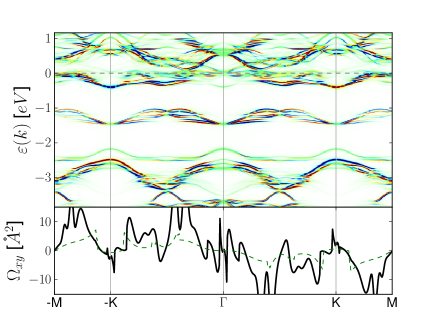
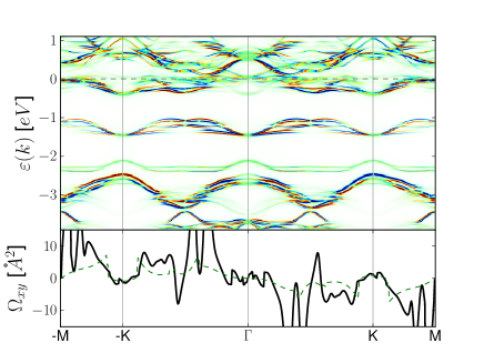
Figure 11: (Color online). Unfolded band structure and Berry curvature of MoS₂ in a $3\times 3$ supercell with two sulfur vacancies at next nearest neighbor sites. Left: ab initio calculation. Right: calculation from effective Hamiltonian constructed from a pristine $3\times 3$ supercell with impurities added in the form of an influence Hamiltonian obtained from a single impurity calculation. The dashed lines show the Berry curvature of pristine MoS₂ with the Fermi level at the indicated position.

We denote pristine band, orbital indices, and crystal momentum by $n,i,\mathbf{k}$ respectively and supercell band, orbital, and crystal momentum indices by $N,I,\mathbf{K}$ respectively. For the present purpose we will use $\mathbf{r}$ for pristine lattice vectors and $\mathbf{R}$ for supercell lattice vectors. We can thus consider the matrix element

$$\langle\psi_{n\mathbf{k}}|\psi_{N\mathbf{K}}\rangle=\sum_{iI\mathbf{r}\mathbf{R}}C^{*}_{ni\mathbf{k}}C_{NI\mathbf{K}}e^{-i\mathbf{k}\cdot(\mathbf{r}+\mathbf{t}_{i})+i\mathbf{K}\cdot(\mathbf{R}+\mathbf{t}_{I})}\langle\varphi_{i\mathbf{r}}|\varphi_{I\mathbf{R}}\rangle$$ (27)

Following Ku et al.ku_unfolding we introduce a map that uniquely identifies orbitals in the supercell with corresponding orbitals in the pristine system. The map thus takes $I\rightarrow\mathbf{r}^{\prime}(I),i^{\prime}(I)$ and we have

$$\langle\varphi_{i\mathbf{k}}|\varphi_{I\mathbf{R}}\rangle=\langle\varphi_{i\mathbf{r}}|\varphi_{i^{\prime}(I)\mathbf{R}+\mathbf{r}^{\prime}(I)}\rangle=\delta_{ii^{\prime}(I)}\delta_{\mathbf{r}\mathbf{R}+\mathbf{r^{\prime}}(I)}.$$ (28)

The matrix element can then be written as

$$\langle\psi_{n\mathbf{k}}|\psi_{N\mathbf{K}}\rangle =\sum_{I\mathbf{R}}C^{*}_{ni^{\prime}(I)\mathbf{k}}C_{NI\mathbf{K}}e^{-i\mathbf{k}\cdot[\mathbf{r}^{\prime}(I)+\mathbf{R}+\mathbf{t}_{{}^{\prime}(I)}]+i\mathbf{K}\cdot[\mathbf{R}+\mathbf{t}_{I}]}$$

$$=\sum_{I}C^{*}_{ni^{\prime}(I)\mathbf{k}}C_{NI\mathbf{K}}e^{-\mathbf{k}\cdot[\mathbf{r}^{\prime}(I)+\mathbf{t}_{i^{\prime}(I)}]+i\mathbf{K}\cdot\mathbf{t}_{I}}\delta_{\mathbf{K}[\mathbf{k}]},$$ (29)

where $[\mathbf{k}]$ is the set of crystal momenta that downfolds to $\mathbf{K}$.

The idea of a map allows one to only work with the supercell system and avoid the explicit calculation of overlap matrices. However, the procedure does require that the supercell system considered is somewhat similar to the pristine reference system and becomes ill-defined if there is not a unique way of relating orbitals in the two systems. Furthermore, it is important to construct the tight-binding Hamiltonian from projected Wannier functions as opposed to maximally localized Wannier functions, since the latter may differ significantly in otherwise similar systems.

In Figs. 5 and 6 we showed examples of the band structures and Berry curvature of MoS₂ in a $3\times 3$ unit cell with a single sulfur vacancy, unfolded onto the normal BZ.

Appendix B Effective Hamiltonians

Here we briefly summarize the construction of effective Hamiltonians as proposed in Ref. berlijn_effective, . In a tight binding framework, the effective Hamiltonian with $N$ impurities is constructed as

$$H^{Eff}_{IJ} (\mathbf{R})=H^{SC}_{IJ}(\mathbf{R})$$ (30)

$$+ \sum_{s=1}^{N}P(I,J,\mathbf{r}_{s},\mathbf{R})H^{\prime}_{i^{\prime}(I)i^{\prime}(J)}(\mathbf{r}^{\prime}(I)-\mathbf{r}_{s},\mathbf{r}^{\prime}(J)+\mathbf{R}-\mathbf{r}_{s}),$$

where $I,J,\mathbf{R}$ denotes a supercell orbitals and lattice vectors respectively. $\mathbf{r}$ is a normal cell lattice vector and $i^{\prime},\mathbf{r}^{\prime}$ are maps from the supercell orbitals and lattice to the normal cell. $\mathbf{r}_{s}$ denotes the position of impurity $s$. The influence Hamiltonian is given by

$$H^{\prime}_{ij}(\mathbf{r}_{1},\mathbf{r}_{2})=H^{Imp}_{ij}(\mathbf{r}_{1},\mathbf{r}_{2})-H^{0}_{ij}(\mathbf{r}_{2}-\mathbf{r}_{1}),$$ (31)

where $H^{Imp}_{i,j}(\mathbf{r}_{1},\mathbf{r}_{2})$ is constructed with a map from the impurity to the normal cell. Since this is expressed in a basis of normal cell lattice vectors $H^{Imp}$ and therefore $H^{\prime}$ is not periodic in simultaneous translations of $\mathbf{r}_{1}$ and $\mathbf{r}_{2}$. We have used the partition function of Liu and Vanderbiltliu_effective

$$P(I,J,\mathbf{r}_{s},\mathbf{R}) =e^{-(d/d_{c})^{8}}$$ (32)

$$d =(|\mathbf{r}^{\prime}(I)-\mathbf{r}_{s}|+|\mathbf{r}^{\prime}(J)+\mathbf{R}-\mathbf{r}_{s}|)/2.$$

with $d_{c}=9.0$ Å.

For applications of the method we have performed ab initio calculations of the pristine and impurity systems and constructed $H^{imp}$ and $H^{0}$ using projected Wannier functions. $H^{SC}$ is then constructed as a straightforward repetition of $H^{0}$.

As a non-trivial test of the method we have performed an ab initio calculation of a $3\times 3$ unit cell of MoS₂ and with sulfur vacancies at two next-nearest neighbor sites. We have then constructed the same system with from the effective Hamiltonian: first we construct obtain the tight binding model of a $3\times 3$ unit cell of MoS₂ by repeating the tight-binding Hamiltonian obtained from a calculations of pristine MoS₂ (normal unit cell). We have then constructed the influence Hamiltonian (31) from the pristine calculation and a calculation of MoS₂ in a $3\times 3$ unit cell with a single sulfur vacancy. The influence Hamiltonian is then added to the $3\times 3$ tight-binding Hamiltonian at the two nearest neighbor sites to obtain the effective Hamiltonian of a system with two impurities. The unfolded bands and curvature of ab initio and effective Hamiltonian calculations are shown in Fig. 11. The unfolded spectral function is nearly indistinguishable in the two case. However, the unfolded Berry curvature is highly sensitive to the exact positions of bands near avoided crossings and therefore exhibits larger deviations in the two methods. Nevertheless, the Berry curvature obtained from the effective Hamiltonian reproduces the main qualitative features (for example a vanishing contribution in the vicinity of $K$ and $-K$) and we believe that the configurational averaged Berry curvature obtained from the effective Hamiltonian methods provides a reliable measure of the effects of disorder on the curvature and VHC.

References

- (1) X. Xu, W. Yao, D. Xiao, and T. F. Heinz, Nat. Phys. 10, 343 (2014)
- (2) K. F. Mak, C. Lee, J. Hone, J. Shan, and T. F. Heinz, Phys. Rev. Lett. 105, 136805 (2010)
- (3) D. Xiao, W. Yao, and Q. Niu, Phys. Rev. Lett. 99, 236809 (2007)
- (4) D. Xiao, G.-B. Liu, W. Feng, X. Xu, and W. Yao, Phys. Rev. Lett. 108, 196802 (2012)
- (5) H. Zeng, J. Dai, W. Yao, D. Xiao, and X. Cui, Nature Nanotech. 7, 490 (2012)
- (6) K. F. Mak, K. He, J. Shan, and T. F. Heinz, Nature Nanotech. 7, 494 (2012)
- (7) T. Cao, G. Wang, W. Han, H. Ye, C. Zhu, J. Shim, Q. Niu, P. Tan, E. Wang, B. Liu, and J. Feng, Nature Comm. 3, 887 (2012)
- (8) D. Xiao, M.-C. Chang, and Q. Niu, Rev. Mod. Phys. 82, 1959 (2010)
- (9) N. Nagaosa, J. Sinova, S. Onoda, A. H. MacDonald, and N. P. Ong, Rev. Mod. Phys. 82, 1539 (2010)
- (10) K. F. Mak, K. L. McGill, J. Park, and P. L. McEuen, Science 344, 1489 (2014)
- (11) N. A. Sinitsyn, Q. Niu, and A. H. MacDonald, Phys. Rev. B 73, 075318 (2006)
- (12) N. A. Sinitsyn, A. H. MacDonald, T. Jungwirth, V. K. Dugaev, and J. Sinova, Phys. Rev. B 75, 045315 (2007)
- (13) W. Zhou, X. Zou, S. Najmaei, Z. Liu, Y. Shi, J. Kong, J. Lou, P. M. Ajayan, B. I. Yakobson, and J.-C. Idrobo, Nano Letters 13, 2615 (2013)
- (14) D. Liu, Y. Guo, L. Fang, and J. Robertson, Applied Physics Letters 103, 183113 (2013)
- (15) Y. Ma, Y. Dai, M. Guo, C. Niu, J. Lu, and B. Huang, Phys. Chem. Chem. Phys. 13, 15546 (2011)
- (16) Y. Zhou, P. Yang, H. Zu, F. Gao, and X. Zu, Phys. Chem. Chem. Phys. 15, 10385 (2013)
- (17) J.-w. Wei, Z.-w. Ma, H. Zeng, Z.-y. Wang, Q. Wei, and P. Peng, AIP Advances 2, 042141 (2012)
- (18) M. Ghorbani-Asl, A. N. Enyashin, A. Kuc, G. Seifert, and T. Heine, Phys. Rev. B 88, 245440 (2013)
- (19) H.-P. Komsa and A. V. Krasheninnikov, Phys. Rev. B 91, 125304 (2015)
- (20) B. Velický, Phys. Rev. 184, 614 (1969)
- (21) J. S. Faulkner and G. M. Stocks, Phys. Rev. B 21, 3222 (1980)
- (22) W. H. Butler, Phys. Rev. B 31, 3260 (1985)
- (23) S. Lowitzer, D. Ködderitzsch, and H. Ebert, Phys. Rev. Lett. 105, 266604 (2010)
- (24) B. Zimmermann, K. Chadova, D. Ködderitzsch, S. Blügel, H. Ebert, D. V. Fedorov, N. H. Long, P. Mavropoulos, I. Mertig, Y. Mokrousov, and M. Gradhand, Phys. Rev. B 90, 220403 (2014)
- (25) J. Kudrnovský, V. Drchal, and I. Turek, Phys. Rev. B 88, 014422 (2013)
- (26) J. Weischenberg, F. Freimuth, J. Sinova, S. Blügel, and Y. Mokrousov, Phys. Rev. Lett. 107, 106601 (2011)
- (27) T. Berlijn, D. Volja, and W. Ku, Phys. Rev. Lett. 106, 077005 (Feb 2011)
- (28) W. Ku, T. Berlijn, and C.-C. Lee, Phys. Rev. Lett. 104, 216401 (May 2010)
- (29) R. Bianco, R. Resta, and I. Souza, Phys. Rev. B 90, 125153 (2014)
- (30) F. D. M. Haldane, Phys. Rev. Lett. 61, 2015 (1988)
- (31) M. Z. Hasan and C. L. Kane, Rev. Mod. Phys. 82, 3045 (2010)
- (32) K. Kaasbjerg, K. S. Thygesen, and K. W. Jacobsen, Phys. Rev. B 85, 115317 (2012)
- (33) F. Hüser, T. Olsen, and K. S. Thygesen, Phys. Rev. B 88, 245309 (2013)
- (34) D. Y. Qiu, F. H. da Jornada, and S. G. Louie, Phys. Rev. Lett. 111, 216805 (2013)
- (35) P. Giannozzi et al., J. Phys.: Condens. Matter 21, 395502 (2009)
- (36) N. Marzari, A. A. Mostofi, J. R. Yates, I. Souza, and D. Vanderbilt, Rev. Mod. Phys. 84, 1419 (Oct 2012)
- (37) I. Souza, N. Marzari, and D. Vanderbilt, Phys. Rev. B 65, 035109 (2001)
- (38) X. Wang, J. R. Yates, I. Souza, and D. Vanderbilt, Phys. Rev. 74, 195118 (2006)
- (39) J. Liu and D. Vanderbilt, Phys. Rev. B 88, 224202 (Dec 2013)