Universal scheme for indirect quantum control
Abstract
We consider a bipartite quantum object, composed of a quantum system and a quantum actuator which is periodically reset. We show that the reduced dynamics of the system approaches unitarity as the reset frequency of the actuator is increased. This phenomenon arises because quantum systems interacting for a short time can impact each other faster than they can become significantly entangled. In the high reset-frequency limit, the effective Hamiltonian describing the system’s unitary evolution depends on the state to which the actuator is reset. This makes it possible to indirectly implement a continuous family of effective Hamiltonians on one part of a bipartite quantum object, thereby reducing the problem of indirect control (via a quantum actuator) to the well-studied one of direct quantum control.
pacs:
03.65.Yz, 03.67.Lx, 03.67.-aI Introduction
Coherent control of quantum systems is a central ingredient for most implementations of quantum computing and metrology. In practice, however, interactions between a controlled quantum system and its environment typically lead to a gradual loss of coherence in the system. It is, therefore, desirable to perform control operations rapidly compared to the system’s coherence times, so as to minimize environment-induced errors. This goal poses a dilemma, since by coupling a system more strongly to a classical controller in order to steer it more quickly, the system may also become coupled more strongly to the general environment, which can then increase its rate of decoherence. Conversely, a system with longer coherence times typically interacts more weakly with all of its surroundings, including a classical controller, making it difficult to control rapidly.
An appealing compromise is to employ indirect control with a setup involving two quantum systems: the to-be-controlled quantum system which is relatively well isolated, coupled to a quantum actuator which is classically controlled and interacts more strongly with the outside world. This strategy has attracted considerable attention since it was found that control of can yield universal control of Lloyd and Viola (2001); Lloyd et al. (2004). Indirect control schemes have shown promise in a variety of settings, including spin chains Burgarth et al. (2009, 2010); Heule et al. (2010), superconducting qubits Strauch (2011), nanomechanical resonators Jacobs (2007); Rabl et al. (2009), and perhaps most notably, in nuclear/electron spin systems Morton et al. (2006, 2008); Hodges et al. (2008); Cappellaro et al. (2009); Taminiau et al. (2014); Aiello and Cappellaro (2015), where they are commonly used. There is, however, no general recipe for mapping a desired unitary on to a series of control operations on which will produce it Jacobs (2007). This is largely due to the entangling nature of the system-actuator coupling; a generic operation on leaves it entangled with , and thus has a net non-unitary effect on the latter.
Physical settings in which a nuclear spin () couples to an electron spin (), such as nitrogen-vacancy (NV) centers and electron spin resonance (ESR) systems, offer an exceptionally convenient way of surmounting this difficulty, as their Hamiltonians can often be cast in the form
| (1) |
where are orthogonal actuator states. The special structure of (1) allows one to evolve unitarily by any , conditioned on the state of Cappellaro et al. (2009); Aiello and Cappellaro (2015); Hodges et al. (2008); Taminiau et al. (2014). This approach—which sidesteps the issue of system-actuator entanglement by working only with states of the latter—reduces the problem of indirect quantum control to the well-studied one of direct control; i.e., of synthesising a desired unitary using a set of available system Hamiltonians Lloyd (1995); Alessandro and Dahleh (2001); Palao and Kosloff (2003); Boscain and Mason (2006); Chakrabarti and Rabitz (2007); Hegerfeldt (2013).
In this paper, we present an explicit scheme for indirect quantum control which employs a resettable actuator to produce unitary evolution of the system, conditioned on the actuator’s state. Crucially, our scheme is completely general in that it can be applied for any and . Furthermore, our scheme does not require any particular form of the - Hamiltonian (e.g., we are not restricted to Hamiltonians of the form (1)), but rather, relies on the ability to reset rapidly. In this sense, it reduces the general problem of indirect control—for any hybrid system—to the much simpler one of direct quantum control.
II The scheme
Consider a quantum system coupled to a quantum actuator . Suppose the pair is initially in the state , and that is periodically reset to at time intervals . (Equivalently, one could couple a succession of fresh actuators to , each prepared in the state .) For convenience, we will assume the resets to be instantaneous, although we shall discuss more realistic resetting later. Between successive resets, - evolves as
| (2) |
where the superoperator is known as a Liouvillian. We decompose into parts describing the free dynamics of and , and the coupling between them:
| (3) |
Here , , and , which act non-trivially on , , and - respectively, are assumed to be time-independent and of Lindblad type Lindblad (1976). We include an arbitrary piecewise-continuous switching function in (3) to demonstrate how time dependence can be incorporated into this scheme. To facilitate comparison with existing indirect control techniques, we will be particularly interested in the case where - evolves unitarily between resets, i.e., where , and .
We encode the effect on of each evolve-and-reset cycle of in the dynamical map , which acts on the system’s density operator as
| (4) |
where denotes the time-ordering operator. We may then write the system’s state after the first cycle as . If is reset times in the interval (so that , where ), the reduced state of at time is , where represents successive applications of the channel .
Our scheme utilizes cycles which are short as compared to the natural dynamics of -. We will therefore seek to expand in powers of , a small number when the actuator is reset at a high rate. In terms of the dynamical map , we wish to find a series of the form
| (5) |
where each is a superoperator that does not depend on . Noting that is independent of (since the argument of is scaled by , see Eq. (3)), we proceed by first expanding asymptotically for small as , where
| (6) |
is a superoperator with no dependence.
Before presenting our main result, let us consider an analogous but simpler situation, namely the case of a matrix representing a rotation by in . The action of can be obtained as the outcome of a series of infinitesimal rotations, each given by , for an arbitrary term. Concretely, setting :
| (7) |
III Main Result
Remarkably, the term in Eq. (5) can be evaluated analogously for any system coupled to a quantum actuator that is repeatedly reset. Specifically, Chernoff’s theorem Chernoff (1968) (p. 241, see also Chernoff (1970, 1976)) gives
| (8) |
This theorem requires that be a continuous function of linear contractions on a Banach space, with . We verify in the Supplemental Material 111See Supplemental Material at http://link.aps.org/supplemental/10.1103/PhysRevA.93.040301 for additional technical details. that , as constructed, satisfies these conditions under the induced trace norm on the set of self-adjoint trace-class operators acting on the system’s Hilbert space.
From Eq. (6), we have that
| (9) |
where gives the average coupling strength between and . Observe that to leading order in , the system evolves as ; therefore, represents an effective Liouvillian for in the limit of frequent actuator resets. We now focus on the case where - is closed (i.e., where the bipartite object evolves unitarily between resets of ). Eq. (9) simplifies to
| (10) |
where
| (11) |
We show explicitly the details of this calculation in the Supplemental Material Note (1). Clearly ; it follows that, to leading order, the system’s reduced dynamics is unitary, and described by
| (12) |
If, for example, the interaction Hamiltonian has the form , the system’s reduced dynamics will be well-described by , where , when the reset rate is high. More generally, different types of coupling between and will lead to different effective Hamiltonians, generating unitary system dynamics conditioned upon . Therefore, by gradually varying the state in which is prepared, one can use this scheme to implement entire families of Hamiltonians on , reducing the problem of indirect control to one of direct quantum control. Moreover, for finite-dimensional systems, our scheme gives universal unitary control of provided and are not related by some symmetry Lloyd (1995).
One can view as receiving a discrete kick from with each cycle. Notice that as ; in other words, as the reset rate becomes large, the kicks to become weaker but more frequent. These competing trends underpin our scheme: When the cycles are short, , i.e., the impact of each kick is mostly encoded in . As in (7), the aggregate effect of many such kicks depends only on to leading order. Crucially though, generically describes a non-trivial, but non-entangling operation on -. This is not unique to our scheme: the non-entangling nature of the first-order Dyson series term has been used in very different contexts, see, e.g., Martín-Martínez et al. (2013). The present scheme, therefore, exploits the general phenomenon that two quantum objects interacting for a short time can impact each other faster than they can become significantly entangled. By mimicking a series of short interactions between and through frequent resets of the latter, we can effectively modify the system’s Hamiltonian without significantly increasing the system’s entropy. Along the same lines, one can also think of the frequent actuator resets as serving to keep in its initial state. The resulting effect is for to evolve according to the portion of the total Hamiltonian acting on the system’s Hilbert space, up to corrections of order .
IV Example
To illustrate our scheme, we consider an archetypal problem in quantum control: that of steering a harmonic oscillator indirectly via a -level actuator . Existing techniques depend crucially on and/or on the nature of the - coupling. For instance, Vogel et al. (1993) requires a Jaynes-Cummings (JC) interaction with , Santos (2005) requires a JC-like coupling with , and Jacobs (2007) requires switching between two distinct interaction Hamiltonians. Our scheme, in contrast, is model-independent. For illustration, however, we pick and an - Hamiltonian
| (13) |
where is a quadrature operator on and . For different choices of , Eq. (13) describes several hybrid objects amenable to indirect quantum control; for example, a nanomechanical resonator coupled to a superconducting qubit Irish and Schwab (2003); Jacobs (2007); LaHaye et al. (2009) or to an electron spin Rabl et al. (2009), as well as circuit (cavity) quantum electrodynamics setups, where an electromagnetic field mode couples to superconducting qubits (atoms).
A direct application of Eq. (11) yields an effective Hamiltonian
| (14) |
on , which is manifestly dependent on . It follows from Lloyd’s well-known argument in Ref. Lloyd (1995) (see also Lloyd and Braunstein (1999)) that any Hamiltonian of the form
| (15) |
can be implemented on by suitably varying the state to which is reset, where .
In implementations, the accuracy with which one can enact evolution by through frequent resets of will be important. To quantify this accuracy, we consider an initial system state and evolve it numerically for a time according to the full Hamiltonian (13), where is reset at a rate . We then compute the fidelity (see caption of Fig. 1 for definition) as a function of , between the resulting reduced system state and the time-evolved state that we wish to obtain. The resulting fidelity is shown in Fig. 1 for three different reset rates.
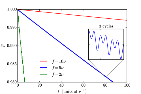
We observe that two qualitatively distinct types of error arise in implementing on with our scheme, see Fig. 1: (i) slowly growing deviation from as increases (apparent in the main panel), and (ii) fast “wiggles” on these otherwise slowly varying curves (shown in the zoomed inset). Type (i) error, which we call dissipative error, arises because and get slightly entangled during cycles of finite duration. Over time, this entanglement causes information about to become lost due to the actuator resets, contributing a non-unitary component to system’s evolution, which accumulates with every cycle. Thus, dissipative error becomes important on long timescales.
Type (ii) error, which we name stroboscopic error, also arises from a finite reset rate ; however, it is important only on comparatively short timescales. When , our scheme approximates smooth evolution by using discrete non-unitary kicks from , which can have complex effects on . Our asymptotic analysis has been focused on the total effect of each kick, described by Eq. (5) for integer . However, the system can display complicated non-unitary dynamics during a cycle of finite duration, the details of which are not described by (nor, more generally, by , , …). Stroboscopic error, then, is the temporary deviation during each cycle between the full open dynamics of and the smooth path described in (5). Because this type of error vanishes at the end of every cycle, it does not accumulate with , and hence, is primarily important over short timescales. We will now establish how both the dissipative and the stroboscopic error decay as the cycle length goes to zero.
V Error analysis
Dissipative error in implementing arises from the , , terms in (5), which generically introduce dissipation into the system’s evolution. These superoperators can be expressed as functions of , , by adapting the method developed in Bentkus (2003) (Section 4). We will use this method to find the form of , the leading-order source of dissipative error.
Consider the function
| (16) |
chosen so that and . Observe that with this definition of we have
| (17) |
One rapidly arrives at expressions for , , by expanding asymptotically in and matching powers with Eq. (5). In particular:
| (18) |
In terms of the reset rate , Eq. (18) scales as . (This statement is readily formalized by noting that the induced trace norm of the integral in (18) is independent of .) The scaling is apparent in Fig. 1, where the reset rates considered are sufficiently high that is the dominant source of dissipative error. In particular, observe that for each plotted, the deviation between the reduced dynamics and the -generated trajectory (corresponding to , the leading-order term in ) is nearly linear in . Furthermore, the slope of the lines scale inversely with .
We now turn our attention to the stroboscopic error. The dynamical map in Eq. (5) describes the system’s evolution for a time , corresponding to an integer number of cycles. In other words, it gives at the end of each cycle. However, between successive resets (i.e., mid-kick), will temporarily stray from the smooth trajectory given in (5).
One can quantify the stroboscopic error by comparing the desired evolution by with the system’s reduced dynamics between successive actuator resets. We use a truncated Dyson series to perform this comparison: If is the system’s state after cycle , then during cycle , evolution by would give
| (19) |
for . When the cycles are short, i.e., when in units set by the largest characteristic frequency of , the terms in the Dyson series will be subdominant, and so we work only to first order in .
Eq. (19) is the evolution our scheme seeks to implement. However, the actual full evolution of between successive resets is computed by evolving - according to and then tracing out the actuator:
| (20) |
Concretely, stroboscopic error is described by the difference between Eqs. (19) and (20):
| (21) | ||||
The braced term in (21) is bounded above in magnitude by , where is the largest coupling strength attained in each cycle. (Thus, stroboscopic error is reduced when the - coupling remains weak.) The commutator, in contrast, can vary arbitrarily with , depending on the nature of . However, it is always suppressed by a prefactor of , and so Eq. (21) generically scales as , which is upper-bounded by . In terms of reset frequency then, stroboscopic error scales as .
Unlike dissipative error, which accumulates with , stroboscopic error vanishes with each reset. Thus, while the former type is reduced by implementing for short durations , the latter can be sidestepped entirely by choosing and to give an integer number of cycles. In general, both types of error can be suppressed arbitrarily by choosing an that is large compared to characteristic frequencies of and .
VI Discussion & Outlook
Our scheme is somewhat reminiscent of the quantum Zeno effect (QZE) Misra and Sudarshan (1977); Facchi and Pascazio (2002); Layden et al. (2015); both our scheme and the QZE feature emergent unitary dynamics generated by an effective Hamiltonian, which results from rapidly repeated operations. However, our scheme does not invoke any type of measurement, nor any notion of “leakage” between measurement eigenstates. Moreover, the QZE typically involves repeated kicks which remain strong (or at least non-vanishing) in the high-frequency limit Facchi and Pascazio (2008). In contrast, the effect on of each individual cycle in our scheme vanishes as . Zanardi and Campos Venuti recently discovered a phenomenon closely related to the QZE, wherein unitary evolution, generated by a “dissipation-projected Hamiltonian”, can arise in an open system. While their results and ours may both stem from a common fundamental principle, the scaling that underpins Refs. Zanardi and Campos Venuti (2014, 2015) is entirely absent in our scheme.
While we have assumed for illustration that is reset instantaneously and at regular intervals, neither of these idealizations are essential to our scheme. Notice from Eq. (9) that does not contribute to ; therefore, would still evolve unitarily by to leading order if were reset through a gradual non-unitary process. We note also that Chernoff’s theorem—which gives the evolution of in the high regime—can be generalized to describe cycles of non-uniform duration. Specifically, when actuator resets are performed in a time , the system’s evolution will be well-described by (or more generally, by ) when the longest time between actuator resets is sufficiently short Smolyanov et al. (1999, 2003).
Finally, we wish to compare our control scheme with the one proposed in Lloyd and Viola (2001): Whereas we employ a resettable quantum actuator to achieve indirect unitary control of a system, Lloyd and Viola used a resettable and measurable ancilla to achieve arbitrary open-system dynamics. The similar requirements of both schemes suggest the possibility of implementing arbitrary open-system dynamics on through indirect control.
VII Acknowledgements
AK, EMM and DL acknowledge support from the NSERC Discovery and NSERC PGSM programs. DL also acknowledges support through the Ontario Graduate Scholarhip (OGS) program. The authors thank Lorenza Viola, Paola Cappellaro, and Daniel Grimmer for helpful discussions.
References
- Lloyd and Viola (2001) S. Lloyd and L. Viola, Phys. Rev. A 65, 010101 (2001).
- Lloyd et al. (2004) S. Lloyd, A. J. Landahl, and J.-J. E. Slotine, Phys. Rev. A 69, 012305 (2004).
- Burgarth et al. (2009) D. Burgarth, S. Bose, C. Bruder, and V. Giovannetti, Phys. Rev. A 79, 060305 (2009).
- Burgarth et al. (2010) D. Burgarth, K. Maruyama, M. Murphy, S. Montangero, T. Calarco, F. Nori, and M. B. Plenio, Phys. Rev. A 81, 040303 (2010).
- Heule et al. (2010) R. Heule, C. Bruder, D. Burgarth, and V. M. Stojanović, Phys. Rev. A 82, 052333 (2010).
- Strauch (2011) F. W. Strauch, Phys. Rev. A 84, 052313 (2011).
- Jacobs (2007) K. Jacobs, Phys. Rev. Lett. 99, 117203 (2007).
- Rabl et al. (2009) P. Rabl, P. Cappellaro, M. V. G. Dutt, L. Jiang, J. R. Maze, and M. D. Lukin, Phys. Rev. B 79, 041302 (2009).
- Morton et al. (2006) J. J. Morton, A. M. Tyryshkin, A. Ardavan, S. C. Benjamin, K. Porfyrakis, S. Lyon, and G. A. D. Briggs, Nature Physics 2, 40 (2006).
- Morton et al. (2008) J. J. Morton, A. M. Tyryshkin, R. M. Brown, S. Shankar, B. W. Lovett, A. Ardavan, T. Schenkel, E. E. Haller, J. W. Ager, and S. Lyon, Nature 455, 1085 (2008).
- Hodges et al. (2008) J. S. Hodges, J. C. Yang, C. Ramanathan, and D. G. Cory, Phys. Rev. A 78, 010303 (2008).
- Cappellaro et al. (2009) P. Cappellaro, L. Jiang, J. S. Hodges, and M. D. Lukin, Phys. Rev. Lett. 102, 210502 (2009).
- Taminiau et al. (2014) T. H. Taminiau, J. Cramer, T. van der Sar, V. V. Dobrovitski, and R. Hanson, Nature nanotechnology 9, 171 (2014).
- Aiello and Cappellaro (2015) C. D. Aiello and P. Cappellaro, Phys. Rev. A 91, 042340 (2015).
- Lloyd (1995) S. Lloyd, Phys. Rev. Lett. 75, 346 (1995).
- Alessandro and Dahleh (2001) D. D. Alessandro and M. Dahleh, Automatic Control, IEEE Transactions on 46, 866 (2001).
- Palao and Kosloff (2003) J. P. Palao and R. Kosloff, Physical Review A 68, 062308 (2003).
- Boscain and Mason (2006) U. Boscain and P. Mason, Journal of Mathematical Physics 47, 062101 (2006).
- Chakrabarti and Rabitz (2007) R. Chakrabarti and H. Rabitz, International Reviews in Physical Chemistry 26, 671 (2007).
- Hegerfeldt (2013) G. C. Hegerfeldt, Phys. Rev. Lett. 111, 260501 (2013).
- Lindblad (1976) G. Lindblad, Communications in Mathematical Physics 48, 119 (1976).
- Gantmacher (1959) F. Gantmacher, The Theory of Matrices, Chelsea Publishing Series (Chelsea, 1959).
- Turin (2004) W. Turin, Performance Analysis and Modeling of Digital Transmission Systems (Kluwer Academic/Plenum Publishers, 2004).
- Chernoff (1968) P. R. Chernoff, J. Funct. Anal. 2, 238 (1968).
- Chernoff (1970) P. R. Chernoff, Bull. Amer. Math. Soc. 76, 395 (1970).
- Chernoff (1976) P. R. Chernoff, Illinois J. Math. 20, 348 (1976).
- Note (1) See Supplemental Material at http://link.aps.org/supplemental/10.1103/PhysRevA.93.040301 for additional technical details.
- Martín-Martínez et al. (2013) E. Martín-Martínez, D. Aasen, and A. Kempf, Phys. Rev. Lett. 110, 160501 (2013).
- Vogel et al. (1993) K. Vogel, V. M. Akulin, and W. P. Schleich, Phys. Rev. Lett. 71, 1816 (1993).
- Santos (2005) M. F. m. c. Santos, Phys. Rev. Lett. 95, 010504 (2005).
- Irish and Schwab (2003) E. K. Irish and K. Schwab, Phys. Rev. B 68, 155311 (2003).
- LaHaye et al. (2009) M. LaHaye, J. Suh, P. Echternach, K. Schwab, and M. Roukes, Nature 459, 960 (2009).
- Lloyd and Braunstein (1999) S. Lloyd and S. L. Braunstein, Phys. Rev. Lett. 82, 1784 (1999).
- Johansson et al. (2013) J. Johansson, P. Nation, and F. Nori, Computer Physics Communications 184, 1234 (2013).
- Bentkus (2003) V. Bentkus, Lithuanian Math. J. 43, 367 (2003).
- Misra and Sudarshan (1977) B. Misra and E. C. G. Sudarshan, Journal of Mathematical Physics 18 (1977).
- Facchi and Pascazio (2002) P. Facchi and S. Pascazio, Phys. Rev. Lett. 89, 080401 (2002).
- Layden et al. (2015) D. Layden, E. Martín-Martínez, and A. Kempf, Phys. Rev. A 91, 022106 (2015).
- Facchi and Pascazio (2008) P. Facchi and S. Pascazio, Journal of Physics A: Mathematical and Theoretical 41, 493001 (2008).
- Zanardi and Campos Venuti (2014) P. Zanardi and L. Campos Venuti, Phys. Rev. Lett. 113, 240406 (2014).
- Zanardi and Campos Venuti (2015) P. Zanardi and L. Campos Venuti, Phys. Rev. A 91, 052324 (2015).
- Smolyanov et al. (1999) O. Smolyanov, H. Weizsäcker, and O. Wittich, in Stochastic Processes, Physics, and Geometry: New Interplays, Proceedings of the Conference on Infinite Dimensional (Stochastic) Analysis and Quantum Physics, Vol. 2 (1999) p. 589.
- Smolyanov et al. (2003) O. Smolyanov, H. Weizsäcker, and O. Wittich, in Evolution Equations: Applications to Physics, Industry, Life Sciences and Economics, Vol. 55 (Birkhäuser, 2003) pp. 349–358.