Two iridates, two models, two approaches:
a comparative study on magnetism in 3D honeycomb materials

Abstract

Two recent theoretical works studied the role of Kitaev interactions in the newly observed incommensurate magnetic order in the hyper-honeycomb ($\beta$-Li₂IrO₃) and stripy-honeycomb ($\gamma$-Li₂IrO₃) iridates. Each of these works analyzed a different model ($JK\Gamma$ versus coupled zigzag chain model) using a contrasting method (classical versus soft-spin analysis). The lack of commonality between these works precludes meaningful comparisons and a proper understanding of these unusual orderings. In this study, we complete the unfinished picture initiated by these two works by solving both models with both approaches for both 3D honeycomb iridates. Through comparisons between all combinations of models, techniques, and materials, we find that the bond-isotropic $JK\Gamma$ model consistently predicts the experimental phase of $\beta$-Li₂IrO₃ regardless of the method used, while the experimental phase of $\gamma$-Li₂IrO₃ can be generated by the soft-spin approach with eigenmode mixing irrespective of the model used. To gain further insights, we solve a 1D quantum spin-chain model related to both 3D models using the density matrix renormalization group method to form a benchmark. We discover that in the 1D model, incommensurate correlations in the classical and soft-spin analysis survive in the quantum limit only in the presence of the symmetric-off-diagonal exchange $\Gamma$ found in the $JK\Gamma$ model. The relevance of these results to the real materials are also discussed.

I Introduction

Lattice	Experimental	Model	Classical	Soft-spin
				no linear combination	with linear combination
$\beta$-LIO	$\mathbf{(A_{a},C_{b},F_{c})}$	$JK\Gamma$	$\mathbf{(A_{a},C_{b},F_{c})}$	$\mathbf{(A_{a},C_{b},F_{c})}$	$\mathbf{(A_{a},C_{b},F_{c})}$
		CZC	Commensurate	$(A_{a},0,F_{c})$	$\mathbf{(A_{a},C_{b},F_{c})}$
$\gamma$-LIO	$\mathbf{(A_{a},F_{b},F_{c})}$	$JK\Gamma$	$(A_{a},C_{b},F_{c})$	$(A_{a},C_{b},F_{c})$	$\mathbf{(A_{a},F_{b},F_{c})}$
		CZC	Commensurate	$(A_{a},0,F_{c})$	$\mathbf{(A_{a},F_{b},F_{c})}$

Table 1: Summary of results for all combinations of model, lattice, and method. The irreducible representations of the $a$, $b$, and $c$ components of the moments in the ground states are given in a shorthand notation. The entry is in bold if the irreducible representations correspond to the experimental phase, i.e. the theoretical phase matches in symmetry with the observed ordering.

Kitaev’s honeycomb model, which hosts an exact $\mathbb{Z}_{2}$ spin liquidKitaev (2006), has been identified to play a crucial role in the low-energy description of the quasi-two-dimensional layered honeycomb iridates $A_{2}$IrO₃ ($A$=Li, Na).Jackeli and Khaliullin (2009); Chaloupka et al. (2010); Singh et al. (2012) A flurry of theoreticalJiang et al. (2011); Reuther et al. (2011); Kimchi and You (2011); You et al. (2012); Schaffer et al. (2012); Price and Perkins (2013); Rau et al. (2014); Katukuri et al. (2014) and experimentalChoi et al. (2012); Ye et al. (2012); Comin et al. (2012); Gretarsson et al. (2013); Cao et al. (2013); Manni et al. (2014); Knolle et al. (2014); Chun et al. (2015) studies have since examined the material’s properties. Most recently, two three-dimensional (3D) analogues of these layered materials have been synthesizedTakayama et al. (2015); Modic et al. (2014), giving hope to being the first realization of a 3D spin liquid. These discoveries have spurred many theoretical studies on the nature of these spin-orbit coupled Mott insulators.Mandal and Surendran (2009); Lee et al. (2014a, b, c); Nasu et al. (2014); Lee and Kim (2015); Kimchi et al. (2014); Kim et al. (2015); Schaffer et al. (2015) However, much like their 2D analogues, these two materials—$\beta$-Li₂IrO₃Biffin et al. (2014a) and $\gamma$-Li₂IrO₃Biffin et al. (2014b) (hereafter $\beta$-LIO and $\gamma$-LIO)—are magnetically ordered rather than exhibiting spin-liquid behavior. To better understand the role of Kitaev physics in these systems, their magnetic behavior must first be scrutinized. As of late, two theoretical studies have attacked the problem from two complementary directions:Lee and Kim (2015); Kimchi et al. (2014) each of these studies proposed a pseudospin 1/2 model describing the low-energy physics of the two iridates and analyzed their respective model using a different approach. The first work examined the $JK\Gamma$ model using a classical approachLee and Kim (2015), while the second analyzed the coupled zigzag chain (CZC) model using a soft-spin methodKimchi et al. (2014) (see Sec. III for definition of the models). The goal of both works is to utilize the detailed experimental magnetic structure to constrain their respective model to the region of the parameter space in which $\beta$-Li₂IrO₃ and $\gamma$-Li₂IrO₃ reside. One common conclusion between the two studies is that the dominance of a ferromagnetic Kitaev term and the presence of subdominant exchange terms (including the antiferromagnetic Heisenberg exchange) generate spiral orders through frustration arising from anisotropic exchanges.

\begin{overpic}[scale={1},clip={true},trim=0.0pt 45.16875pt 0.0pt 45.16875pt]{h0_lattice.pdf} \put(12.2,0.7){$\scriptsize{x}$} \put(15.1,3.0){$\scriptsize{y}$} \put(6.3,12.0){$\scriptsize{z}$} \put(22.0,22.9){$\scriptsize{1}$} \put(33.2,22.5){$\scriptsize{2}$} \put(40.6,26.6){$\scriptsize{4}$} \put(51.5,26.1){$\scriptsize{3}$} \end{overpic}

(a)

\begin{overpic}[scale={1},clip={true},trim=0.0pt 45.16875pt 0.0pt 45.16875pt]{h1_lattice.pdf} \put(12.2,0.7){$\scriptsize{x}$} \put(15.1,3.0){$\scriptsize{y}$} \put(6.3,12.0){$\scriptsize{z}$} \put(24.4,19.8){$\scriptsize{1^{\prime}}$} \put(35.4,19.5){$\scriptsize{2^{\prime}}$} \put(59.0,18.7){$\scriptsize{4^{\prime}}$} \put(69.6,18.2){$\scriptsize{3^{\prime}}$} \put(20.0,13.5){$\scriptsize{1}$} \put(41.0,26.0){$\scriptsize{2}$} \put(51.8,25.5){$\scriptsize{4}$} \put(72.0,11.6){$\scriptsize{3}$} \end{overpic}

(b)

Figure 1: (Color online) Lattices of the hyper- and stripy-honeycomb. The red and green bonds are the symmetry-equivalent $X$ and $Y$ bonds. The blue bonds are the $Z$ bonds, which are symmetry-inequivalent to the $X/Y$ bonds. For the stripy-honeycomb lattice, there are two inquivalent sets of $Z$ bonds. The bonds between black sites are the $Z_{1}$ bonds while the bonds between red sites are the $Z_{2}$ bonds. The labeling of these bonds correspond to the Ising component present in the definition of the Kitaev interactions in both the $JK\Gamma$ and CZC models. The numbers indicate the sublattice labeling used in this work.

While both works unearthed certain features of the magnetism in these new iridates, their approaches and results have important differences. Without a reliable method of solving a frustrated quantum spin model in three dimensions, a definitive evaluation of these two models and methods is beyond reach. All hope is not lost, however: a careful comparison of the models and techniques used can offer a much more cohesive and encompassing understanding of the magnetism in these 3D honeycomb iridates.

In this study, we complete the picture depicted in these previous works by examining the $JK\Gamma$ and CZC models using both classical and soft-spin approaches. This work compares all combinations of models and methods, culminating in an understanding greater than the sum of its parts. Our main result is summarized in Table 1, where we compare the resulting ground states of all eight combinations of materials, methods, and models. With these results, we conclude that the $JK\Gamma$ model on the hyper-honeycomb is most robust as it predicts the experimental phase under all methods. Additionally, we find that the $\gamma$-LIO magnetic structure can only be captured with the soft-spin approach with linear combination of multiple eigenmodes in both the $JK\Gamma$ and CZC models.

Ultimately, to understand how each of these methods succeeds or fails to capture the quantum ground state properties, a comparison with a quantum treatment would be highly desirable. However, these frustrated quantum mechanical spin models are difficult to solve in three dimensions. Hence, we analyze a 1D spin-chain model that is related to both the $JK\Gamma$ and CZC models. In one dimension, the quantum solution of the spin model was obtained numerically using the density matrix renormalization group (DMRG) technique. We compare the classical solution and soft-spin analysis with the quantum results and find that incommensurate correlations found in both classical and soft-spin methods only persist in the quantum limit when the symmetric off-diagonal exchange $\Gamma$ is finite. Although useful as an illustrative tool, we also caution the extrapolation of these results to higher dimensions, noting that quantum models can behave drastically differently as the dimensionality of the system changes.

In Sec. II, we briefly provide background information on the two iridates in question: the hyper-honeycomb $\beta$-LIO and the stripy-honeycomb $\gamma$-LIO. In Sec. III, we outline the differences between the two spin models—the $JK\Gamma$ and the CZC models. Then, in Sec. IV, we delve into the details of the classical and soft-spin approaches, applying these methods to obtain phase diagrams for the two models at hand. We conclude this section with a discussion about the implications of our findings. We present our 1D spin chain results in Sec. V, and relate these results to those obtained earlier for the 3D models. Lastly in Sec. VI, we provide a summary of our results and an outlook on the topic of magnetism in these 3D iridate materials.

II Two iridates

The two 3D honeycomb iridates are structural variants (polymorphs) of Li₂IrO₃, and the elementary building blocks of both compounds is the IrO₆ octahedron. Each octahedron shares three edges with its three neighbors, defining a tri-coordinated network of Ir ions. The resulting networks differ between the two compounds, as seen in Fig. 1. Distinguishing features include the number of symmetry-inequivalent nearest-neighbor (NN) bonds and the symmetries they possess. In the hyper-honeycomb, there are only two symmetry-inequivalent sets of bonds: the $X/Y$ bonds that possesses inversion symmetry and the $Z$ bonds that possesses $222$ point group symmetry. In contrast, there are three symmetry-inequivalent sets of NN bonds in the stripy-honeycomb: the $X/Y$ bonds that do not possess any symmetry, the $Z_{1}$ bonds that possess $2/m$ symmetry, and the $Z_{2}$ bonds that possess $222$ symmetry. These distinctions are important in the construction of models for these materials and in results discussed in Sec. IV.3.

The magnetism found in these two iridates have many striking similarities. Both materials undergo a magnetic phase transition at $T\sim 38~{}K$.Takayama et al. (2015); Modic et al. (2014) The magnetic order in both cases is a non-coplanar, incommensurate spiral order, where moments on neighboring sublattices rotate in the opposite sense (also known as counter-rotation of spirals). Moreover, the wavevector of both spirals are equal within experimental resolution: $\sim$(0.57,0,0) in the $hkl$ notation of each compound’s respective orthorhombic unit cell.Biffin et al. (2014a, b)

While very similar, differences in the detailed magnetic structure have been identified.Biffin et al. (2014a, b) In the hyper-honeycomb case, the spiral order transforms under a single irreducible representation (irrep) of the magnetic space group: $\Gamma_{4}$ (see Appendix A for details).Biffin et al. (2014a) In other words, when applied to the spiral order, all symmetries of the lattice that leaves the ordering wavevector $\sim(0.57,0,0)$ invariant results in a factor of $\pm 1$, where the sign is dictated by the character of the irreducible representation. In contrast, the spiral in the stripy-honeycomb case transforms in a more complicated fashion: the moments parallel to the orthorhombic $b$ direction transform under a different irrep ($\Gamma_{3}$) than the moments perpendicular to the $b$ direction ($\Gamma_{4}$).Biffin et al. (2014b) Alternatively, in terms of magnetic basis vectors, this implies that the magnetic structure of $\beta$-LIO transforms as $(A_{a},C_{b},F_{c})$ while the magnetic structure of $\gamma$-LIO transforms as $(A_{a},F_{b},F_{c})$. This subtle difference between the two spiral orders is outlined in the first two columns of Table 1 and plays a crucial role in our discussion when comparing the two models and the two methods.

III Two models

A low-energy description of these Mott insulators with strong SOC can be obtained by starting in the atomic picture. In this limit, the partially-filled Ir⁴⁺ ions are in the $5d^{5}$ configuration. In the presence of large octahedral crystal fields and strong SOC, an effective low-energy description can be derived from a single electron occupying the high-energy $j_{\text{eff}}=1/2$ doublet. In the Mott insulating limit, the low-energy degrees of freedom of these half-filled doublets can be represented by $j_{\text{eff}}=1/2$ pseudospins. Due to the strong SOC, these pseudospins are expected to interact via strongly anisotropic exchanges (i.e. strong exchange-anisotropy). This is supported by perturbative calculations that capture both the effects of virtual states in the presence of Hund’s coupling and oxygen-mediated superexchange mechanisms. We now explore two pseudospin models motivated by these symmetry considerations.

III.1 $JK\Gamma$ model

The $JK\Gamma$ model proposed in Ref. Lee and Kim, 2015 assumes that all bonds have the same exchange parameters (bond-isotropy). In addition, the model assumes all bonds take on three exchange parameters $J$, $K$, and $\Gamma$, resulting in the Hamiltonian

$$H=\sum_{\langle ij\rangle\in\alpha\beta(\gamma)}\left[J\vec{S}_{i}\cdot\vec{S}_{j}+KS^{\gamma}_{i}S^{\gamma}_{j}+e^{i\theta_{ij}}\Gamma S^{\alpha}_{i}S^{\beta}_{j}\right],$$ (1)

where the pseudospin at site $i$ is denoted as $\vec{S}_{i}$, NN bonds are denoted as $\langle ij\rangle$, and each NN bond is labelled by $\gamma\in(X,Y,Z)$. The shorthand $\langle ij\rangle\in\alpha\beta(\gamma)$ means $\langle ij\rangle\in\gamma$ and an implicit sum is taken over only $\alpha$ and $\beta$ where $\alpha\neq\beta\neq\gamma$. The phase angle $\theta_{ij}\in\{0,\pi\}\text{ mod }2\pi$ is bond-dependent and is partially constrained by the symmetry of the lattice. In the model considered in Ref. Lee and Kim, 2015 and here, it is given by $\theta_{ij}=\pi(\hat{r}_{ij}\cdot\vec{v}+1)$ where $\hat{r}_{ij}$ is the unit vector from site $i$ to $j$, $\vec{v}=\frac{1}{\sqrt{2}}(\frac{\vec{b}}{4}+\frac{\vec{c}}{6})$, and $\vec{b}$, $\vec{c}$ are the conventional lattice vectors.

III.2 Coupled zigzag chain model

The coupled zigzag chain (CZC) model proposed in Ref. Kimchi et al., 2014 assumes that the $X/Y$ bonds and $Z$ are distinct (for $\gamma$-LIO, $Z_{2}$ and $Z_{1}$ bonds are assumed to possess the same exchange parameters). Hence, this is an intrinsically bond-anisotropic model. Furthermore, the number of exchange parameters have been restricted: while the $Z$ bonds ($Z_{2}$ and $Z_{1}$ bonds in $\gamma$-LIO) are assumed to have three parameters similar to the $JK\Gamma$ model, the $X/Y$ bonds possess only two exchanges that parametrize the Heisenberg and Kitaev exchanges. These exchanges are related as the $X/Y$ bonds and $Z$ bonds share the same $J$ and $K$ values via

$$H=\sum_{\langle ij\rangle\in\gamma}[J\vec{S}_{i}\cdot\vec{S}_{j}+KS^{\gamma}_{i}S^{\gamma}_{j}]+\sum_{\langle ij\rangle\in Z}I_{c}(\hat{r}_{ij}\cdot\vec{S}_{i})(\hat{r}_{ij}\cdot\vec{S}_{j}).$$

In the above, $\langle ij\rangle$ denotes NN sites, $J,K,I_{c}$ are the Heisenberg, Kitaev, and Ising couplings respectively, $\gamma$ is the Kitaev component and label on bond $ij$, $\hat{r}_{ij}$ is the unit vector from site $i$ to $j$, and the Ising term only sums over the $Z$ bonds. One can also re-write the exchanges in terms of the $JK\Gamma$ parametrization on each bond to manifestly show the bond-anisotropy

$$J_{Z}=J+\frac{1}{2}I_{c} K_{Z}=K-\frac{1}{2}I_{c} \Gamma_{Z}=\frac{1}{2}I_{c}$$

$$J_{X/Y}=J K_{X/Y}=K \Gamma_{X/Y}=0,$$

where the bond label of each exchange is indicated by the subscript.

IV Two approaches

\begin{overpic}[scale={.93},clip={true},trim=0.0pt 0.0pt 0.0pt 0.0pt]{h0_jkg_classical} \put(64.0,90.0){$\scriptsize{\phi=0}$} \put(62.0,28.0){$\scriptsize{\frac{7\pi}{4}}$} \put(0.0,7.0){$\scriptsize{\frac{3\pi}{2}}$} \put(15.0,25.0){\color[rgb]{0,0,0}\line(-1,2){5.0}} \put(20.0,22.0){\color[rgb]{0,0,0}\line(2,-1){12.0}} \put(40.0,45.0){\rotatebox[origin={c}]{40.0}{$\scriptsize{\frac{5\pi}{8}}$}} \put(27.5,60.5){\rotatebox[origin={c}]{40.0}{$\scriptsize{\frac{3\pi}{4}}$}} \put(15.0,76.0){\rotatebox[origin={c}]{40.0}{$\scriptsize{\frac{7\pi}{8}}$}} \put(39.0,71.0){AF${}_{a}$} \put(4.0,51.0){NCsp${}_{a}$} \put(4.0,38.0){NCsp${}_{b}$} \put(30.0,9.0){SS${}_{b}$} \end{overpic}

(a)

\begin{overpic}[scale={.93},clip={true},trim=0.0pt 0.0pt 0.0pt 0.0pt]{h0_jkg_soft} \put(64.0,90.0){$\scriptsize{\phi=0}$} \put(62.0,28.0){$\scriptsize{\frac{7\pi}{4}}$} \put(0.0,7.0){$\scriptsize{\frac{3\pi}{2}}$} \put(15.0,25.0){\color[rgb]{0,0,0}\line(-1,2){5.0}} \put(40.0,45.0){\rotatebox[origin={c}]{40.0}{$\scriptsize{\frac{5\pi}{8}}$}} \put(27.5,60.5){\rotatebox[origin={c}]{40.0}{$\scriptsize{\frac{3\pi}{4}}$}} \put(15.0,76.0){\rotatebox[origin={c}]{40.0}{$\scriptsize{\frac{7\pi}{8}}$}} \put(39.0,71.0){AF${}_{a}$} \put(4.0,51.0){NCsp${}_{a}$} \put(4.0,38.0){NCsp${}_{b}$} \end{overpic}

(b)

\begin{overpic}[scale={.93},clip={true},trim=0.0pt 0.0pt 0.0pt 0.0pt]{h1_jkg_classical} \put(64.0,90.0){$\scriptsize{\phi=0}$} \put(62.0,28.0){$\scriptsize{\frac{7\pi}{4}}$} \put(0.0,7.0){$\scriptsize{\frac{3\pi}{2}}$} \put(40.0,45.0){\rotatebox[origin={c}]{40.0}{$\scriptsize{\frac{5\pi}{8}}$}} \put(27.5,60.5){\rotatebox[origin={c}]{40.0}{$\scriptsize{\frac{3\pi}{4}}$}} \put(15.0,76.0){\rotatebox[origin={c}]{40.0}{$\scriptsize{\frac{7\pi}{8}}$}} \put(39.0,71.0){AF${}_{a}$} \put(4.0,51.0){NCsp${}_{a}$} \put(15.6,22.3){\rotatebox[origin={c}]{15.0}{SS${}_{x/y}$}} \put(31.0,34.0){SS${}_{b}$} \end{overpic}

(c)

\begin{overpic}[scale={.93},clip={true},trim=0.0pt 0.0pt 0.0pt 0.0pt]{h1_jkg_soft} \put(64.0,90.0){$\scriptsize{\phi=0}$} \put(62.0,28.0){$\scriptsize{\frac{7\pi}{4}}$} \put(0.0,7.0){$\scriptsize{\frac{3\pi}{2}}$} \put(18.0,22.0){\color[rgb]{0,0,0}\line(3,-1){7.0}} \put(24.0,40.0){\color[rgb]{0,0,0}\line(3,2){18.0}} \put(24.0,33.0){\color[rgb]{0,0,0}\line(2,-1){20.0}} \put(40.0,45.0){\rotatebox[origin={c}]{40.0}{$\scriptsize{\frac{5\pi}{8}}$}} \put(27.5,60.5){\rotatebox[origin={c}]{40.0}{$\scriptsize{\frac{3\pi}{4}}$}} \put(15.0,76.0){\rotatebox[origin={c}]{40.0}{$\scriptsize{\frac{7\pi}{8}}$}} \put(39.0,71.0){AF${}_{a}$} \put(4.0,51.0){NCsp${}_{a}$} \put(42.0,17.0){NCsp${}_{b}$} \put(40.0,54.0){NCsp${}_{a}^{\prime}$} \put(15.2,22.1){\rotatebox[origin={c}]{15.0}{AF${}_{ac}$}} \put(34.0,34.0){SS${}_{b}$} \end{overpic}

(d)

Figure 2: (Color online) $JK\Gamma$ model: comparing the classical and soft-spin (with no mixing) approaches on the hyper-honeycomb and stripy-honeycomb lattices. The classical approach stipulates the constant-spin-length constraint whereas the soft-spin approach does not. LT fails in the region bounded by the red dotted line. The non-coplanar spiral (NCsp_a) state exist in all phase diagrams—it is the experimentally observed phase in the hyper-honeycomb $\beta$-LIO and closely related to the experimental phase in the stripy-honeycomb $\gamma$-LIO. The values at the circle boundary are $\phi$-values, whereas values inside are $\theta$-values; see Eq. 2 and surrounding main text for parametrization used.

\begin{overpic}[scale={.93},clip={true},trim=0.0pt 0.0pt 0.0pt 0.0pt]{h0_czc_classical.pdf} \put(0.8,95.0){$\frac{J}{|K|}$} \put(84.0,8.0){$\frac{I_{c}}{K}$} \put(38.0,70.0){SS${}_{b}$} \put(70.0,20.0){FM${}_{c}$} \put(65.0,52.0){SS${}_{x/y}$} \put(6.0,13.5){$0$} \put(1.0,30.0){$0.1$} \put(1.0,47.0){$0.2$} \put(1.0,63.0){$0.3$} \put(1.0,80.0){$0.4$} \put(12.0,8.0){$0$} \put(23.0,8.0){$0.2$} \put(38.0,8.0){$0.4$} \put(53.0,8.0){$0.6$} \put(68.0,8.0){$0.8$} \end{overpic}

(a)

\begin{overpic}[scale={.93},clip={true},trim=0.0pt 0.0pt 0.0pt 0.0pt]{h0_czc_soft.pdf} \put(0.8,95.0){$\frac{J}{|K|}$} \put(84.0,8.0){$\frac{I_{c}}{K}$} \put(38.0,70.0){SS${}_{b}$} \put(70.0,20.0){FM${}_{c}$} \put(65.0,52.0){Csp${}_{a}$} \put(6.0,13.5){$0$} \put(1.0,30.0){$0.1$} \put(1.0,47.0){$0.2$} \put(1.0,63.0){$0.3$} \put(1.0,80.0){$0.4$} \put(12.0,8.0){$0$} \put(23.0,8.0){$0.2$} \put(38.0,8.0){$0.4$} \put(53.0,8.0){$0.6$} \put(68.0,8.0){$0.8$} \end{overpic}

(b)

Figure 3: (Color online) CZC model: comparing the classical and soft-spin (with no mixing) approaches on the hyper-honeycomb and stripy-honeycomb lattices. The hyper- and stripy-honeycomb results agree within each method hence only one figure is shown per method. LT fails in the region bounded by the red dotted line. The classical method finds commensurate ordering in the whole parameter space considered, whereas the soft-spin approach finds a coplanar spiral in the LT-failed region. See text for additional details on phases present and discussion on the comparison.

In the two studies Ref. Lee and Kim, 2015 and Kimchi et al., 2014, not only were the models considered different, the approaches used to identify the ground states of each model also differed. Here we first provide details on both methods then subsequently complete the analysis of the prior studies by applying both methods to both models on the two iridates in consideration.

IV.1 Classical analysis

In the classical limit, the quantum mechanical pseudospins are treated as constant length vectors. For $S=1/2$, the classical treatment is equivalent to a variational method where the ansatz is restricted to a site-factorized product state. This is because the product state ansatz must satisfy the classical unit length constraint due to the unique Bloch sphere nature of $S=1/2$ spins: the expectation value $\langle\vec{S}\rangle$ for any pure state forms a constant length vector. As such, to capture long-range ordered states, the classical approach is a useful first method to employ.

To solve the classical problem (or equivalently, the variational problem), we have various tools at our disposal. The Luttinger-Tisza (LT) approximation is an important method that serves to provide a lower bound to the classical ground state energy and it also identifies the exact classical ground state when the method succeeds. Success is defined as finding a solution that satisfies the constant spin-length constraint across all sites and is typically met in regions of parameter space where geometrical and/or exchange frustration is minimal.

Procedurally, the essence of the LT method involves taking a Fourier transform of the real-space exchange Hamiltonian into momentum-space and diagonalizing the resultant matrix at all momenta to yield an LT band structure. Then, we identify the momenta that globally minimize such band structure and examine the corresponding degenerate eigenspace. Lastly, we attempt to construct an eigenvector within the degenerate eigenspace that, when Fourier transformed back into real-space, yields a constant spin-length configuration. If such a configuration is found, then the state is a classical ground state and the energy corresponds to the state’s eigenvalue. If no such configuration can be found, the LT method is deemed to have failed and the lowest eigenvalue is the lower bound to the classical ground state energy. In the regions of parameter space where LT fails, we in turn employ numerical methods such as simulated annealing to find the classical ground state, supplemented with the knowledge of the lower bound in the classical energy from the LT analysis.

IV.1.1 Previous results from $JK\Gamma$ model

We first review the classical results of the $JK\Gamma$ model. In Fig. 2a and 2c, we reproduce the classical phase diagram of the $JK\Gamma$ model for both 3D honeycomb systems from Ref. Lee and Kim, 2015 with $J\geq 0$, $K\leq 0$, and $\Gamma\leq 0$, which contains the experimentally relevant spiral phases. The exchange interactions are parametrized in the polar plot as

$$(J,K,\Gamma)=(\sin\theta\cos\phi,\sin\theta\sin\phi,\cos\theta),$$ (2)

where $\phi$ is the angular coordinate and $r=(\pi-\theta)$ is the radial coordinate. As such, the outer edge of the quarter-circle is the Heisenberg-Kitaev limit, the left edge is the $J=0$ limit, and the top edge is the $K=0$ limit. Outside the red dotted lines, LT succeeds and an antiferromagnetic phase (AF_a) exists. Within the red dotted lines, LT fails and we subsequently employed simulated annealing to identify the ground states in this outlined region.

Hyper-honeycomb:

The NCsp_a (Non-Coplanar spiral) phase in the dotted region reproduces the experimentally observed magnetic order. It is a non-coplanar, counter-rotating spiral order with the experimentally observed broken symmetries and an ordering wavevector in the $h00$ direction. In terms of the magnetic basis vectors, the NCsp_a phase transforms as $(A_{a},C_{b},F_{c})$, i.e. as a single-irrep $\Gamma_{4}$. The ordering wavevector in the NCsp_a region continuously changes as a function of $J$, $K$, and $\Gamma$, and the experimental wavevector is contained within. In addition to the NCsp_a phase, there is also another non-coplanar spiral with wavevector in the $0k0$ direction (NCsp_b) and a skew-stripy phase (SS_b).

Stripy-honeycomb:

In contrast to the hyper-honeycomb case, none of the phases in the stripy-honeycomb phase diagram reproduces the experimental phase exactly, although the NCsp_a phase in the stripy-honeycomb model is similar to the experimental phase. In particular, the NCsp_a phase transforms as the single irrep $\Gamma_{4}$ with symmetry $(A_{a},C_{b},F_{c})$, which differs from the experimental phase in the $b$ component. Like the hyper-honeycomb case, the wavevectors in the NCsp_a region continuously change as a function of the exchange parameters and the region contains the experimental wavevector.

For further details on the classical results for the $JK\Gamma$ model including the existence of other magnetic orders and other parameter regimes, we refer the reader to Ref. Lee and Kim, 2015.

IV.1.2 New results from CZC model

In Fig. 3a, we applied the classical analysis on the CZC model for both the hyper-honeycomb and stripy-honeycomb lattices in the same parameter region as that of Ref. Kimchi et al., 2014, i.e. $0\leq J\leq 0.5$, $K=-1$, and $0\geq I_{c}\geq-1.0$. The phase diagrams of both the hyper- and stripy-honeycomb CZC model yield identical phase boundaries and hence only one phase diagram is shown. Outside the red dotted region where either the Heisenberg exchange ($J$) or the Ising exchange ($I_{c}$) dominates, LT succeeds and identifies two distinct commensurate phases. In the large $J/|K|$ region, the ground state is a skew-stripy phase (SS_b), while in the large $I_{c}/K$ region, a collinear ferromagnetic ground state (FM_c) in the $c$ direction is found.

In the dotted region where LT fails, simulated annealing identifies commensurate ground states. The FM_c phase that was found in the large $I_{c}/K$ region enlarges into the dotted region, and a new skew-stripy phase (SS_a/b) emerges between the FM_c and SS_b phase. The experimental spiral phase does not appear in the classical analysis of the CZC model in either crystal structures.

IV.2 Soft-spin analysis

In the soft-spin analysis as proposed in Ref. Kimchi et al., 2014, one initially follows the same procedure as the LT method as outlined in Sec. IV.1, but disregards the constant spin-length constraint. It was suggested that the minimum eigenvalue solution, which may violate the spin-length constraint, can be considered as a soft-spin solution.Kimchi et al. (2014) If the constant spin-length condition is satisfied, however, the solution will be the same as the classical solution. It was further proposed that one can construct a more complex spin structure with the same wavevector by forming a linear combination, or mixing, of the lowest and certain higher-eigenvalue eigenvectors, which may be considered as a potential candidate solution for the quantum model.Kimchi et al. (2014) Here we will follow their prescription and investigate the results in both models.

IV.2.1 Previous results from CZC model

In Fig. 3b, we reproduced the soft-spin phase diagram obtained in Ref. Kimchi et al., 2014, which applies to both hyper- and stripy-honeycomb CZC models. As explained in Sec. IV.2, the difference between the classical and soft-spin results lies within the dotted region where LT fails. In this region, the soft-spin analysis finds the Csp_a phase with a continuously changing wavevector as a function of $J/|K|$ and $I_{c}/K$. This phase is a coplanar, counter-rotating spiral with vanishing moments along the orthorhombic $b$ direction and a wavevector along the $h00$ direction.

This state differs from the experimental phase because moments are only in the $a$-$c$ plane, hence yielding the symmetry $(A_{a},0,F_{c})$ ($0$ is used to denote the vanishing $b$ component). To obtain a finite component along the $b$ direction while ensuring the symmetry of the experimental phase, the eigenvector of the fifth-lowest eigenvalue was linearly combined with the eigenvectors of the lowest eigenvalue.Kimchi et al. (2014) This mixed state has the symmetry $(A_{a},C_{b},F_{c})$ in the case of the hyper-honeycomb, and $(A_{a},F_{b},F_{c})$ in the case of the stripy-honeycomb, in agreement with experimental results.Kimchi et al. (2014) It was proposed that this mixture of eigenvectors would result in a candidate solution for the quantum model.Kimchi et al. (2014)

IV.2.2 New results from $JK\Gamma$ model

In Fig. 2b and 2d, we have computed the phase diagram of the $JK\Gamma$ model using the soft-spin approach. For both the hyper-honeycomb and stripy-honeycomb cases, in the region where one would find the NCsp_a phase using the classical approach, we find phases with the same broken symmetry albeit with modified ordering wavevector lengths and non-constant spin-lengths. In this region of both lattices, the ordering wavevector continuously changes and contains the experimentally verified wavevector.

Hyper-honeycomb:

The symmetry of this lowest-eigenvalue state is $(A_{a},C_{b},F_{c})$, and since it agrees with the experimental phase, a linear combination with higher-eigenvalue eigenvectors is not necessary. In other words, the $JK\Gamma$ model on the hyper-honeycomnb lattice succeeds in finding the experimental phase in both the classical analysis and the soft-spin analysis (without mixture). In comparison with the classical results, both the NCsp_a and NCsp_b phases enlarge and meets the boundary of where LT fails. The SS_b phase that was found in the classical analysis does not appear in the soft-spin analysis.

Stripy-honeycomb:

The lowest-eigenvalue state has symmetry $(A_{a},C_{b},F_{c})$, which is identical to the NCsp_a phase in the classical analysis. A state with the experimental symmetry $(A_{a},F_{b},F_{c})$ can be obtained if higher-eigenvalue eigenvectors are mixed, similar to the results outlined above for the CZC model. In addition to this phase, there are also two additional non-coplanar spirals, NCsp${}_{a}^{\prime}$ and NCsp_b, and a non-coplanar, commensurate, antiferromagnetic phase, AF_ac. NCsp${}_{a}^{\prime}$ has an ordering wavevector along the $h00$ direction but has a different symmetry from NCsp_a. On the other hand, NCsp_b has an ordering wavevector along the $0k0$ direction in analogy to the similarly named phase in the hyper-honeycomb phase diagram. The non-coplanar, commensurate antiferromagnetic phase AF_ac lies close to the Kitaev limit and is distinct from the SS_x/y phase predicted in the classical analysis. This phase consists of moments aligned antiferromagnetically in the $c$ direction on the $Z_{1}$ bonds, and antiferromagnetically in the $a$ direction on the $Z_{2}$ bonds with a small ferromagnetic component along the $b$ axis. Overall, the phase does not have a net moment as the ferromagnetic tilts on the various $Z_{2}$ bonds within the unit cell are anti-aligned.

IV.3 Discussion

Table 1 summarizes our main results and allows for an easy comparison between all methods, models, and lattices at a glance. The table lists the symmetry of the experimentally observed ordering for each lattice, followed by the symmetry of the generated phases present for each model using classical analysis and the soft-spin analysis with and without mixing of eigenmodes.

In the $\beta$-LIO case, the $JK\Gamma$ model generates the experimental phase under all methods in consideration. In contrast to the robustness of the $JK\Gamma$ model, the CZC model can only generate the experimental phase under the soft-spin approach with mixing of eigenmodes. Since the $JK\Gamma$ model is manifestly bond-isotropic while the CZC model is not, this difference in robustness in generating the experimental phase may be attributed to the bond-isotropy of the real material. The bond-isotropy of $\beta$-LIO is supported by the near-ideal Ir-Ir and Ir-O bond lengths and Ir-O-Ir bond anglesTakayama et al. (2015) in addition to the bond-isotropic orbital overlaps observed in recent ab initio results.Kim et al. (2015) For the $\gamma$-LIO case, the soft-spin approach with mixing of eigenmodes can generate the experimental phase using both the $JK\Gamma$ and CZC models. However, none of the models can generate the experimental phase within the classical approach or the soft-spin approach without linear combination of eigenmodes. This may also be related to the more distorted nature of the $\gamma$-LIO lattice as observed by structural analysis,Modic et al. (2014) which may imply large bond-anisotropies in the effective spin model. These anisotropies together with the absence of any symmetry on the $X/Y$ bonds suggests that other symmetry-allowed, subdominant exchanges not yet accounted for in either the $JK\Gamma$ or CZC model may be important in determining the ground state in the real material. To assess these possibilities, ab initio studies like DFT or quantum chemistry calculations may provide the necessary insights and are thus crucial in our understanding of $\gamma$-LIO.

As noted in Sec. IV.1, the classical solution, as determined by LT or by any other method, yields a definite variational wavefunction and variational energy of the quantum spin-$1/2$ model. At the cost of obtaining a definite wavefunction and energy, the classical approach ignores all quantum effects. Although the classical approach may correctly generate the broken symmetries deep within the long-range ordered phases, near phase boundaries where quantum fluctuations may be enhanced, this approach may fail to identify the correct broken symmetries (if there are any) of the ground state. It may also be possible that the classical approach fails completely when quantum fluctuations are sufficiently large that the long-range order is destroyed. Despite these shortcomings, some quantum corrections to the wavefunction and energy in addition to the stability of the phases can be partially accounted for via spin-wave theory or Jastrow factors in variational Monte Carlo schemes.

It was suggestedKimchi et al. (2014) that the soft-spin approach may generate spin structures that incorporate the effects of quantum fluctuations. The procedure of forming linear combination of multiple eigenmodes allows for construction of more complex ordering at the same wavevector. As a trade-off, the resulting expectation value of the Hamiltonian using this soft-spin state (in both unmixed and mixed cases) cannot be interpreted as a variatonal energy and the obtained spin structure cannot be readily translated into a wavefunction. Therefore, whether the classical or soft-spin result is favoured in a quantum treatment at finite or zero temperature cannot be determined within these two methods alone and a comparison with a quantum treatment would be ideal. However, the study of such 3D frustrated quantum spin models is currently computationally prohibitive, especially when searching for incommensurate phases. Therefore, to gather more insight regarding the methods and models considered thus far, we consider a 1D spin chain limit of both the $JK\Gamma$ and CZC models, which can be tackled by the DMRG technique.

V 1D spin chain model

\begin{overpic}[scale={.93},clip={true},trim=0.0pt 0.0pt 0.0pt 0.0pt]{1d_jkg_dmrg.pdf} \put(64.0,90.0){$\scriptsize{\phi=0}$} \put(62.0,28.0){$\scriptsize{\frac{7\pi}{4}}$} \put(0.0,7.0){$\scriptsize{\frac{3\pi}{2}}$} \put(40.0,45.0){\rotatebox[origin={c}]{40.0}{$\scriptsize{\frac{5\pi}{8}}$}} \put(27.5,60.5){\rotatebox[origin={c}]{40.0}{$\scriptsize{\frac{3\pi}{4}}$}} \put(15.0,76.0){\rotatebox[origin={c}]{40.0}{$\scriptsize{\frac{7\pi}{8}}$}} \put(12.0,50.0){Sp} \put(45.0,73.0){AF} \end{overpic}

(a)

\begin{overpic}[scale={.93},clip={true},trim=0.0pt 0.0pt 0.0pt 0.0pt]{1d_czc_dmrg.pdf} \put(0.8,93.0){$\frac{J_{1}}{|K|}$} \put(80.0,8.0){$\frac{J_{2}}{|K|}$} \put(49.0,71.0){a} \put(49.0,51.0){b} \put(46.0,79.0){AF} \put(46.0,30.0){FM} \put(72.0,63.0){ST} \put(6.0,15.0){$0$} \put(1.0,30.0){$0.1$} \put(1.0,47.0){$0.2$} \put(1.0,63.0){$0.3$} \put(1.0,80.0){$0.4$} \put(3.0,8.0){$-0.24$} \put(28.0,8.0){$-0.16$} \put(53.0,8.0){$-0.08$} \end{overpic}

(b)

\begin{overpic}[scale={.93},clip={true},trim=0.0pt 0.0pt 0.0pt 0.0pt]{1d_jkg_classical.pdf} \put(64.0,90.0){$\scriptsize{\phi=0}$} \put(62.0,28.0){$\scriptsize{\frac{7\pi}{4}}$} \put(0.0,7.0){$\scriptsize{\frac{3\pi}{2}}$} \put(40.0,45.0){\rotatebox[origin={c}]{40.0}{$\scriptsize{\frac{5\pi}{8}}$}} \put(27.5,60.5){\rotatebox[origin={c}]{40.0}{$\scriptsize{\frac{3\pi}{4}}$}} \put(15.0,76.0){\rotatebox[origin={c}]{40.0}{$\scriptsize{\frac{7\pi}{8}}$}} \put(12.0,50.0){Sp} \put(45.0,73.0){AF} \end{overpic}

(c)

\begin{overpic}[scale={.93},clip={true},trim=0.0pt 0.0pt 0.0pt 0.0pt]{1d_czc_classical.pdf} \put(0.8,93.0){$\frac{J_{1}}{|K|}$} \put(80.0,8.0){$\frac{J_{2}}{|K|}$} \put(36.0,74.0){AF} \put(36.0,30.0){FM} \put(66.0,56.0){ST} \put(48.0,52.0){Sp} \put(6.0,15.0){$0$} \put(1.0,30.0){$0.1$} \put(1.0,47.0){$0.2$} \put(1.0,63.0){$0.3$} \put(1.0,80.0){$0.4$} \put(3.0,8.0){$-0.24$} \put(28.0,8.0){$-0.16$} \put(53.0,8.0){$-0.08$} \end{overpic}

(d)

\begin{overpic}[scale={.93},clip={true},trim=0.0pt 0.0pt 0.0pt 0.0pt]{1d_jkg_soft.pdf} \put(64.0,90.0){$\scriptsize{\phi=0}$} \put(62.0,28.0){$\scriptsize{\frac{7\pi}{4}}$} \put(0.0,7.0){$\scriptsize{\frac{3\pi}{2}}$} \put(40.0,45.0){\rotatebox[origin={c}]{40.0}{$\scriptsize{\frac{5\pi}{8}}$}} \put(27.5,60.5){\rotatebox[origin={c}]{40.0}{$\scriptsize{\frac{3\pi}{4}}$}} \put(15.0,76.0){\rotatebox[origin={c}]{40.0}{$\scriptsize{\frac{7\pi}{8}}$}} \put(12.0,50.0){Sp} \put(45.0,73.0){AF} \end{overpic}

(e)

\begin{overpic}[scale={.93},clip={true},trim=0.0pt 0.0pt 0.0pt 0.0pt]{1d_czc_soft.pdf} \put(0.8,93.0){$\frac{J_{1}}{|K|}$} \put(80.0,8.0){$\frac{J_{2}}{|K|}$} \put(36.0,74.0){AF} \put(36.0,30.0){FM} \put(66.0,56.0){ST} \put(48.0,52.0){Sp} \put(6.0,15.0){$0$} \put(1.0,30.0){$0.1$} \put(1.0,47.0){$0.2$} \put(1.0,63.0){$0.3$} \put(1.0,80.0){$0.4$} \put(3.0,8.0){$-0.24$} \put(28.0,8.0){$-0.16$} \put(53.0,8.0){$-0.08$} \end{overpic}

(f)

Figure 4: (Color online) Phase diagram of 1D spin-chain model in the decoupled $JK\Gamma$ limit ($\Gamma<0$, $J_{2}=0$) and decoupled CZC limit ($\Gamma=0$, $J_{2}<0$) obtained via three different methods. The regions enclosed by the red dotted lines indicate that LT failed. In a), c), and e), we studied the decoupled $JK\Gamma$ limit with DMRG, classical, and soft-spin analysis respectively. Similarly, in b), d), and f), we simulated the decoupled CZC limit. In the decoupled $JK\Gamma$ limit, all three methods predict an incommensurate phase (Sp) and an antiferromagnetic (AF) phase. These phases are found in analogous positions in parameter space compared to the 3D $JK\Gamma$ models in Fig. 2. In the decoupled CZC limit, there are three commensurate phases: away from the stripy (ST) phase at small $J_{2}$, a ferromagnet (FM) and antiferromagnet (AF) appear. The classical d) and soft-spin f) analyses also predict an intermediate incommensurate spiral (Sp) phase that does not appear in the quantum analysis. The dotted lines in b) are cuts for which we show the structure factor in Fig. 5; the structure factor peaks for $\theta=\frac{3\pi}{4}$ in a) are shown in Fig. 6.

The 1D spin chain model related to both the $JK\Gamma$ and CZC models is an extension of the spin chain model considered in Ref. Kimchi et al., 2014. It is given by

$$H= \sum_{\langle ij\rangle\in\alpha\beta(\gamma)}J_{1}\vec{S}_{i}\cdot\vec{S}_{j}+KS^{\gamma}_{i}S^{\gamma}_{j}+e^{i\theta_{ij}}\Gamma S^{\alpha}_{i}S^{\beta}_{j}$$

$$+\sum_{\langle\langle ij\rangle\rangle}J_{2}\vec{S}_{i}\cdot\vec{S}_{j},$$ (3)

where only $X$ and $Y$ bonds are included in the sums, $\langle\langle ij\rangle\rangle$ denotes second nearest neighbors (2NN), and the phase factor appearing before $\Gamma$ is defined identically to Eq. 1. When $\Gamma\neq 0$ and $J_{2}=0$, we arrive at the decoupled limit of the $JK\Gamma$ model: it is identical to Eq. 1 with vanishing $Z$ bond exchanges, resulting in decoupled chains with only $X/Y$ bonds. When $\Gamma=0$ and $J_{2}=0$, we similarly reach the decoupled limt of the CZC model. The 2NN Heisenberg exchange has been introduced to this decoupled CZC limit in Ref. Kimchi et al., 2014 to compensate for the loss of the $Z$ bond exchanges.Kimchi et al. (2014) By studying these two limits with all three approaches—DMRG, classical, and soft-spin analysis—we aim to compare the three methods and to understand the essential ingredient needed to generate incommensurate correlations. A more in-depth discussion of the DMRG results can be found in Appendix B.

In the decoupled $JK\Gamma$ limit, Fig. 4 shows that all three approaches capture incommensurate correlations. This shows that the spiral correlations generated by the frustration between the $\Gamma$ term and the HK terms persist in the quantum limit. We notice that the classical and soft-spin analysis yield similar phase boundaries that coincide with the area where LT fails (enclosed by the red dotted lines), while in the quantum limit, the incommensurate region enlarges beyond the red dotted lines. On the contrary, in the decoupled CZC limit, we find that the quantum phase diagram obtained via DMRG does not contain the incommensurate correlations predicted by both the classical and soft-spin analysis. In particular, the commensurate phases are captured by all three methods (quantum, classical, and soft-spin), but an intermediate spiral phase is only present in the classical and soft-spin analysis within the region where LT fails. This suggests that the incommensurate correlations driven by the 2NN Heisenberg is ultimately disfavoured by quantum effects. Taken together, these two sets of results suggests that finite $\Gamma$, and not further neighbor interactions, can stablize incommensurate correlations in the 1D limit.

One may hypothesize that the same trend will occur in the 3D models discussed in this work: in the quantum limit, the Csp_a phase predicted using the soft-spin approach in the CZC model for both lattices may be disfavoured relative to the commensurate phases due to the absence of $\Gamma$ along the chain direction. However, since quantum effects in 1D systems are typically greater than 3D systems, this extrapolation of results remains speculative. Future studies are needed to establish the connection between these 1D decoupled chain results and the quantum phase diagram of the 3D models.

VI Summary

We have completed the picture initated in two previous works by examining both the $JK\Gamma$ and CZC models using both the classical and soft-spin approaches. For the hyper-honeycomb, the robustness of the $JK\Gamma$ model in predicting the experimental phase regardless of the method used suggests that bond-isotropic interactions can explain the observed spiral order. On the other hand, the experimental phase of $\gamma$-LIO can only be reproduced using the soft-spin analysis with mixing of eigenmodes using both $JK\Gamma$ and CZC models, suggesting that further investigations are needed to deduce an effective model from microscopic origins. In all cases where the experimental phase was predicted, a dominant ferromagnetic Kitaev exchange exists as a common thread. We conclude by examining the decoupled limit of both the $JK\Gamma$ and CZC models and observed that a finite $\Gamma$ was needed to ensure that the incommensurate correlations predicted in both the classical and soft-spin methods persist in the quantum limit. Further exploration extending these findings to higher dimensions are warranted in order to assess the relevance of these results to the 3D honeycomb iridates.

Appendix A Magnetic basis vectors

The irreducible representations and magenetic basis vectors for a magnetic structure with ordering wavevector $\vec{q}=(h00)$ in the orthorhombic unit cell of the hyper-honeycomb lattice are given byBiffin et al. (2014a)

Irreducible	Basis
Representation	Vectors
$\Gamma_{1}$	$F_{a}$, $G_{b}$, $A_{c}$
$\Gamma_{2}$	$C_{a}$, $A_{b}$, $G_{c}$
$\Gamma_{3}$	$G_{a}$, $F_{b}$, $C_{c}$
$\Gamma_{4}$	$A_{a}$, $C_{b}$, $F_{c}$

In the sublattice basis given in Fig. 1a, the magnetic basis vectors are given byBiffin et al. (2014a)

$$F=\begin{bmatrix}1\\ 1\\ 1\\ 1\\ \end{bmatrix},C=\begin{bmatrix}1\\ 1\\ -1\\ -1\\ \end{bmatrix},A=\begin{bmatrix}1\\ -1\\ -1\\ 1\\ \end{bmatrix},G=\begin{bmatrix}1\\ -1\\ 1\\ -1\\ \end{bmatrix}.$$ (4)

With a structure specified by the basis vectors $\vec{v}=(iv_{a},iv_{b},v_{c})$, the moments at each site is given byBiffin et al. (2014a)

$$\vec{S}_{n}(\vec{r}) =\hat{a}S_{a}v_{a}(n)\sin\vec{q}\cdot\vec{r}+\hat{b}S_{b}v_{b}(n)\sin\vec{q}\cdot\vec{r}$$

$$+\hat{c}S_{c}v_{c}(n)\cos\vec{q}\cdot\vec{r},$$ (5)

where $\hat{a}$, $\hat{b}$, $\hat{c}$ are the unit vectors of the orthorhombic lattice vectors, $\vec{S}_{n}(\vec{r})$ is the moment at position $\vec{r}$ which has sublattice index $n$, and $S_{i}$ are the magnitudes of each component of the moment. Since all phases predicted in this work have relative phases between components given by $\vec{v}=(iv_{a},iv_{b},v_{c})$, we adopt a shorthand notation by dropping the relative imaginary unit $i$: $\vec{v}\equiv(v_{a},v_{b},v_{c})$.

For the stripy-honeycomb, there are 8 sublattices in the unit cell as opposed to 4 for the hyper-honeycomb. We break up those 8 sublattices into two sets of 4—the unprimed $1-4$ sublattices and the primed sublattices $1^{\prime}-4^{\prime}$ as seen in Fig. 1b.Biffin et al. (2014b) The irreducible representations and magnetic basis vectors for wavevector $h00$ are given byBiffin et al. (2014b)

Irreducible	Basis
Representation	Vectors
$\Gamma_{1}$	$C_{a}$, $A_{b}$, $G_{c}$
$\Gamma_{2}$	$F_{a}$, $G_{b}$, $A_{c}$
$\Gamma_{3}$	$A_{a}$, $C_{b}$, $F_{c}$
$\Gamma_{4}$	$G_{a}$, $F_{b}$, $C_{c}$

The magnetic basis vectors are also specified by Eq. 4. The structure given by

$$\vec{v}=i(v_{a},-v^{\prime}_{a}),i(v_{b},-v^{\prime}_{b}),(v_{c},v^{\prime}_{c})$$ (6)

is also specified by Eq. A but with a relative sign on the $a$ and $b$ components between the primed and unprimed sublattices. Since all magnetic structures predicted in this work has the relative phases given by Eq. 6, we adopt the shorthand notation where $\vec{v}\equiv(v_{a},v_{b},v_{c})$.

Appendix B 1D spin chain results

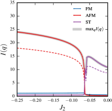
(a)

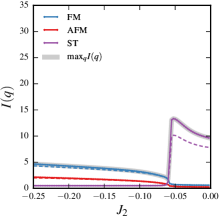
(b)

Figure 5: Decoupled CZC model: specific cuts of the static structure factor $I(q)=\sum_{\mu}I^{\mu\mu}(q)$ for $q=0$ (FM), $\pi/2$ (ST) and $\pi$ (AF) are shown in (a-b) for $N=128$ (solid lines) and $N=96$ (dashed lines). Along with these we shown the maximum of $I(q)$, which always belongs to one of these three choices.

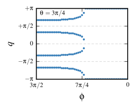
Figure 6: Decoupled $JK\Gamma$ model: location of the maximum static structure factor (i.e. $\text{max}_{q}[I(q)=\sum_{\mu}I^{\mu\mu}(q)]$) for $\theta=3\pi/4$ as a function of $\phi$ for the $N=128$ case. The antiferromagnetic phase for $\phi\gtrsim 7\pi/4$ has the maximum peak located at $\pm\pi$. Below this value of $\phi$, incommensurate correlations develop and persist down to $\phi=3\pi/2$.

To determine the ground state phase diagram of Eq. (V), we used the DMRG as implemented in the ITensor framework.ITe We consider a chain of $N\leq 128$ sites with open boundary conditions. In the decoupled $JK\Gamma$ limit where $J_{2}=0$, we parameterize our phase diagram in the same manner as per Eq. 2. In the decoupled CZC limit where $\Gamma=0$, we fix the energy scale $K=-1$ such that there is a two-dimensional parameter space $(J_{1},J_{2})$ to explore. For each point in parameter space we perform 10-20 sweeps, keeping up to $1000$ states resulting in a maximum truncation error of $\sim 10^{-9}$. For small system sizes ($N\leq 22$) these results were checked for consistency against exact diagonalization.

To characterize the phases we consider two diagnostics: derivatives of the ground state energy and the static structure factor. Sharp features in the energy derivatives signal phase boundaries while peaks in the diagonal components of the static structure factor

$$I^{\mu\mu}({q})\equiv\frac{1}{N}\sum_{ij}e^{i{q}\cdot(i-j)}\langle S^{\mu}_{i}S^{\mu}_{j}\rangle,$$ (7)

signal the ordering wave-vector.

For the decoupled CZC model, we find that throughout the entire phase diagram the maxima of the structure factor $I(q)$ appear only at wave-vectors $q=0$, $\pi/2$ or $\pi$ corresponding to a ferromagnet (FM-$xy$), antiferromagnet (AF-$z$) or stripy (ST) phase. The isotropic structure factor $I\equiv\sum_{\mu}I^{\mu\mu}(q)$ for each of these wave-vectors is shown in Fig. 5 for both $N=96$ and $N=128$. The ferromagnet and stripy phases primarily have correlations in the $\hat{x}$ and $\hat{y}$ directions with the maxima in appearing in $I^{xx}$ or $I^{yy}$, while the anti-ferromagnet is oriented in the $\hat{z}$ direction, with the corresponding maximum in $I^{zz}$.

The gross features of this phase diagram can be understood easily. First we have two exactly solvable points present in the $J_{2}=0$ limit; the Kitaev chain at $J_{1}=0$ and a point dual to a Heisenberg ferromagnet at $J_{1}=1/2$. As in the two-dimensional case, a stripy phase extends between these two solvable points. This is stable to finite $J_{2}$, but ultimately gives way to either the FM-$xy$ or the AF-$z$ phases. These can be understood by considering the large $J_{2}$ limit where the even and odd sites decouple into two ferromagnetic chains. The relative orientation of the two sublattices is then determined by the $K$ and $J_{1}$ interactions, with $K<0$ favouring ferromagnetism and $J_{1}>0$ favouring anti-ferromagnetism.

The anti-ferromagnetic phase for $J_{1}\gtrsim 0.3$ can also be understood by considering the solvable point at $(J_{1},J_{2})=(1/2,0)$. This point is dual to the ferromagnetic Heisenberg point via a four-sublattice transformation, and hence possesses SU$(2)$ spin rotation symmetry in the rotated basis. One finds this continuous degeneracy is broken by finite $J_{2}$, selecting the AF-$z$ state as the ground state, which is a simple product state. Since this product state is the ground state of the ferromagnetic $J_{2}$ interaction and the $(J_{1},K)=(1/2,-1)$ interaction independently, it follows that this product state is the exact ground state of the $(J_{1},K,J_{2})=(1/2,-1,J_{2})$ line. As $J_{1}$ decreases, the AF correlations are preserved but the ground state is no longer a simple product state.

For the decoupled $JK\Gamma$ model, we find one boundary across the phase diagram as indicated by energy derivatives. The maxima of the structure factor of the phase connected to the antiferromagnetic Heisenberg point is located at $\pm\pi$, indicating AF correlations. As we move across the boundary to the adjacent region, peaks in the structure factor develop at incommensurate wavevectors while the peak at $\pm\pi$ vanishes. This incommensurate peak’s position varies as we approach the $J_{1}=0$ limit. The stripy phase located in the $\Gamma=0$ limit does not extend into the finite $\Gamma$ region, in contrast to the effects of $J_{2}$ in the decoupled CZC model. We illustrate the position of the maximum of the static structure factor for $\theta=3\pi/4$ as a function of $\phi$ in Fig. 6.