On eigenvalue accumulation for non-self-adjoint magnetic operators

Abstract.

In this work, we use regularized determinants to study the discrete spectrum generated by relatively compact non-self-adjoint perturbations of the magnetic Schrödinger operator $(-i\nabla-\textbf{{A}})^{2}-b$ in ${\mathbb{R}}^{3}$, with constant magnetic field of strength $b>0$. The distribution of the above discrete spectrum near the Landau levels $2bq$, $q\in\mathbb{N}$, is more interesting since they play the role of thresholds of the spectrum of the free operator. First, we obtain sharp upper bounds on the number of complex eigenvalues near the Landau levels. Under appropriate hypothesis, we then prove the presence of an infinite number of complex eigenvalues near each Landau level $2bq$, $q\in\mathbb{N}$, and the existence of sectors free of complex eigenvalues. We also prove that the eigenvalues are localized in certain sectors adjoining the Landau levels. In particular, we provide an adequate answer to the open problem from [34] about the existence of complex eigenvalues accumulating near the Landau levels. Furthermore, we prove that the Landau levels are the only possible accumulation points of the complex eigenvalues.

1. Introduction and motivations

Presently, there is an increasing interest of mathematical physics community in the spectral theory of non-self-adjoint differential operators. Several results on the discrete spectrum generated by non-self-adjoint perturbations have been established for the quantum Hamiltonians. Still, most of them give Lieb-Thirring type inequalities or upper bounds on certain distributional characteristics of eigenvalues, [15, 5, 4, 9, 10, 19, 16, 42, 7, 34, 12] (for an extensive reference list on the subject, see for instance the references given in [42, 7]). Otherwise, results on spectral properties on non-self-adjoint operators can be found in the article by Sjöstrand [38] and the references given there. In most of the above papers, the non-trivial question of the existence of complex eigenvalues near the essential spectrum is not treated and stays open.

For instance, in [42], Wang studied $-\Delta+V$ in $L^{2}\big{(}{\mathbb{R}}^{n}\big{)}$, $n\geq 2$, where the potential $V$ is dissipative. That is,

(1.1) $$V(x)=V_{1}(x)-iV_{2}(x),$$

where $V_{1}$ and $V_{2}$ are two measurable functions such that $V_{2}(x)\geq 0$, and $V_{2}(x)>0$ on an open non empty set. He showed that if the potential decays faster than $|x|^{-2}$, then the origin is not an accumulation point of the complex eigenvalues. For more general complex potentials without sign restriction on the imaginary part, it is still unknown whether the origin can be an accumulation point of complex eigenvalues or not. In this connection, the author [35] proves the existence of complex eigenvalues near the Landau levels together with their localization property for non-self-adjoint two-dimensional Schrödinger operators with constant magnetic field.

Motivated by Wang’s work [42], the current paper is devoted to the same type of results on eigenvalues near the Landau levels for the three-dimensional Schrödinger operator with constant magnetic field. Now, the essential spectrum of the operator under consideration equals ${\mathbb{R}}_{+}$, and the Landau levels play the role of thresholds. Consequently, the situation is more complicated than the non-self-adjoint case of the two-dimensional Schrödinger operator studied in [35], where the essential spectrum coincides with the (discrete) set of the Landau levels.

The magnetic field B is generated by the magnetic potential $\textbf{A}=(-\frac{bx_{2}}{2},\frac{bx_{1}}{2},0)$. Namely, $\textbf{B}=\text{curl}\hskip 2.84544pt\textbf{A}=(0,0,b)$ with constant direction, where $b>0$ is a constant giving the strength of the magnetic field. Then, the magnetic Schrödinger operator is defined by

(1.2) $$H_{0}:=(-i\nabla-\textbf{A})^{2}-b=\left(-i\frac{\partial}{\partial x_{1}}+\frac{b}{2}x_{2}\right)^{2}+\left(-i\frac{\partial}{\partial x_{2}}-\frac{b}{2}x_{1}\right)^{2}+\left(-i\frac{\partial}{\partial x_{3}}\right)^{2}-b,$$

in $L^{2}({\mathbb{R}}^{3})$ with $x=(x_{1},x_{2},x_{3})\in{\mathbb{R}}^{3}$. Actually, $H_{0}$ is the self-adjoint operator associated with the closure $\overline{q}$ of the quadratic form

(1.3) $$q(u)=\int_{{\mathbb{R}}^{3}}\left(\big{|}(-i\nabla-\textbf{A})u(x)\big{|}^{2}-b|u(x)|^{2}\right)dx,$$

originally defined on $C_{0}^{\infty}({\mathbb{R}}^{3})$. The form domain $D(\overline{q})$ of $\overline{q}$ is the magnetic Sobolev space $H_{\textbf{A}}^{1}({\mathbb{R}}^{3}):=\big{\{}u\in L^{2}({\mathbb{R}}^{3}):(-i\nabla-\textbf{A})u\in L^{2}({\mathbb{R}}^{3})\big{\}}$, (see for instance [23]). Setting $X_{\perp}:=(x_{1},x_{2})\in{\mathbb{R}}^{2}$ and $L^{2}({\mathbb{R}}^{3})=L^{2}({\mathbb{R}}_{X_{\perp}}^{2})\otimes L^{2}({\mathbb{R}}_{x_{3}})$, $H_{0}$ can be rewritten in the form

(1.4) $$H_{0}=H_{\rm Landau}\otimes I_{3}+I_{\perp}\otimes\left(-\frac{\partial^{2}}{\partial x_{3}^{2}}\right).$$

Here,

(1.5) $$H_{\text{Landau}}:=\left(-i\frac{\partial}{\partial x_{1}}+\frac{b}{2}x_{2}\right)^{2}+\left(-i\frac{\partial}{\partial x_{2}}-\frac{b}{2}x_{1}\right)^{2}-b$$

is the shifted Landau Hamiltonian, self-adjoint in $L^{2}({\mathbb{R}}^{2})$, and $I_{3}$, $I_{\perp}$ are the identity operators in $L^{2}({\mathbb{R}}_{x_{3}})$ and $L^{2}({\mathbb{R}}_{X_{\perp}})$ respectively. It is well known (see for instance [1, 11]) that the spectrum of $H_{\text{Landau}}$ consists of the so-called Landau levels $\Lambda_{q}:=2bq$, $q\in{\mathbb{N}}:=\{0,1,2,\ldots\}$, and ${\rm dim}\,{\rm Ker}(H_{\text{Landau}}-\Lambda_{q})=\infty$. Hence,

$$\sigma(H_{0})=\sigma_{\rm ac}(H_{0})=[0,+\infty),$$

and, once again, the Landau levels play the role of thresholds of this spectrum.

Remark 1.1.

Looking at (1.4) as well as the structure of the spectrum of $H_{\text{Landau}}$ and the one of $-\frac{\partial^{2}}{\partial x_{3}^{2}}$, one sees that the structure of $H_{0}$ is quite close to the one of the (free) quantum waveguide Hamiltonians.

Let us introduce some important definitions. Let $M$ be a closed linear operator acting on a separable Hilbert space $\mathscr{H}$. If $z$ is an isolated point of $\sigma(M)$, the spectrum of $M$, let $\gamma$ be a small positively oriented circle centred at $z$ and containing $z$ as the only point of $\sigma(M)$.

Definition 1.1 (Discrete eigenvalue).

The point $z$ is said to be a discrete eigenvalue of $M$ if its algebraic multiplicity is finite and

(1.6) $$\text{mult}(z):=\text{rank}\left(\frac{1}{2i\pi}\int_{\gamma}(M-\zeta)^{-1}d\zeta\right).$$

Note that we have $\text{mult}(z)\geq\text{dim}\big{(}\text{Ker}(M-z)\big{)}$, the geometric multiplicity of $z$. The inequality becomes an equality if $M$ is self-adjoint.

Definition 1.2 (Discrete spectrum).

The discrete spectrum of $M$ is defined by

(1.7) $$\sigma_{\textup{{disc}}}(M):=\big{\{}z\in{\mathbb{C}}:z\hskip 2.84544pt\textup{{is a discrete eigenvalue of} $M$}\big{\}}.$$

Definition 1.3 (Essential spectrum).

The essential spectrum of $M$ is defined by

(1.8) $$\sigma_{\textup{{ess}}}(M):=\big{\{}z\in{\mathbb{C}}:\textup{$M-z$ {is not a Fredholm operator}}\big{\}}.$$

It is a closed subset of $\sigma(M)$.

The purpose of this paper is to investigate the distribution of the discrete spectrum near the essential spectrum of the perturbed operator

(1.9) $$H:={H_{0}}+W\qquad\text{on}\qquad Dom({H_{0}}),$$

where $W:{\mathbb{R}}^{3}\longrightarrow{\mathbb{C}}$ is a non-self-adjoint relatively compact perturbation with respect to $H_{0}$. In (1.9), $W$ is identified with the multiplication operator by the function (also denoted) $W$. In the sequel, $W$ is supposed to satisfy some general assumptions (see (1.13) ).

To put our results in perspective, let us first discuss known results in the case of self-adjoint perturbations. It is well known (see for instance [1, Theorem 1.5]) that if $W:{\mathbb{R}}^{3}\longrightarrow{\mathbb{R}}$ satisfies

(1.10) $$W(x)\leq-C{\bf 1}_{U}(x),\qquad x\in{\mathbb{R}}^{3},$$

for some constant $C>0$ and some non-empty open set $U\subset{\mathbb{R}}^{3}$, then the discrete spectrum of $H$ is infinite. Moreover, if $W$ is axisymmetric ($i.e.$ depends only on $|X_{\perp}|$ and $x_{3}$) and verifies (1.10), then it is known (see for instance [1, Theorem 1.5]) that $H$ has an infinite number of eigenvalues embedded in the essential spectrum. In the case where $W$ is axisymmetric verifying

(1.11) $$W(x)\leq-C{\bf 1}_{S}(X_{\perp})(1+|x_{3}|)^{-m_{3}},\qquad m_{3}\in(0,2),\qquad x=(X_{\perp},x_{3})\in{\mathbb{R}}^{3},$$

for some constant $C>0$ and some non-empty open set $S\subset{\mathbb{R}}^{2}$, it is also proved (see [30, 31]) that below each Landau level $2bq,q\in{\mathbb{N}}$, there is an infinite sequence of discrete eigenvalues of $H$ converging to $2bq$. In [2, 3], the resonances of the operator $H$ near the Landau levels have been investigated for self-adjoint potentials $W$ decaying exponentially in the direction of the magnetic field. Namely,

(1.12) $$W(x)=\mathcal{O}\big{(}(1+|X_{\perp}|)^{-m_{\perp}}\exp\big{(}-N|x_{3}|\big{)},\qquad x=(X_{\perp},x_{3})\in{\mathbb{R}}^{3},$$

with $m_{\perp}>0$ and $N>0$. Other results on the distribution of discrete spectrum for magnetic quantum Hamiltonians perturbed by self-adjoint electric potentials can be found in [20, Chap. 11-12], [26, 27, 28, 25, 39, 40, 33] and the references therein.

Throughout this paper, our minimal assumption on $W$ defined by (1.9) is the following:

(1.13) $$\textit{{Assumption (A1):}}\begin{cases}\bullet\hskip 1.70717ptW\in L^{\infty}({\mathbb{R}}^{3},{\mathbb{C}}),W(x)=\mathcal{O}\big{(}F(X_{\perp})G(x_{3})\big{)},x=(X_{\perp},x_{3})\in{\mathbb{R}}^{3},\\ \bullet\hskip 1.70717ptF\in\bigl{(}L^{\frac{p}{2}}\cap L^{\infty}\bigr{)}\big{(}{\mathbb{R}}^{2},{\mathbb{R}}_{+}^{\ast}\big{)}\hskip 1.13809pt\textup{for some $p\geq 2$},\\ \bullet\hskip 1.70717pt{\mathbb{R}}_{+}^{\ast}\ni G(x_{3})=\mathcal{O}\big{(}\langle x_{3}\rangle^{-m}\big{)},m>3,\end{cases}$$

where $\langle y\rangle:=\sqrt{1+|y|^{2}}$ for $y\in{\mathbb{R}}^{d}$.

Remark 1.2.

Typical example of potentials satisfying Assumption (A1) is the special case of potentials $W:{\mathbb{R}}^{3}\rightarrow{\mathbb{C}}$ such that

(1.14) $$W(x)=\mathcal{O}\big{(}\langle X_{\perp}\rangle^{-m_{\perp}}\langle x_{3}\rangle^{-m}\big{)},\quad m_{\perp}>0,\quad m>3.$$

We can also consider the class of potentials $W:{\mathbb{R}}^{3}\rightarrow{\mathbb{C}}$ such that

(1.15) $$W(x)=\mathcal{O}\big{(}\langle\textup{{x}}\rangle^{-\alpha}\big{)},\quad\alpha>3.$$

Indeed, condition (1.15) implies that (1.14) holds for any $m\in(3,\alpha)$ and $m_{\perp}=\alpha-m>0$.

Under Assumption (A1), we establish (see Lemma 3.1) that the weighted resolvent $|W|^{\frac{1}{2}}({H_{0}}-z)^{-1}$ belongs to the Schatten-von Neumann class ${\mathcal{S}_{p}}$ (see Subsection 3.1 where the classes ${\mathcal{S}_{p}}$, $p\geq 1$ are introduced). Consequently, $W$ is relatively compact with respect to ${H_{0}}$. Then, from Weyl’s criterion on the invariance of the essential spectrum, it follows that

(1.16) $$\sigma_{\text{{ess}}}({H})=\sigma_{\text{{ess}}}({H_{0}})=[0,+\infty).$$

However, the electric potential $W$ may generate (complex) discrete eigenvalues ($\sigma_{\text{{disc}}}({H})$) that can only accumulate to $\sigma_{\text{{ess}}}({H})$, see [18, Theorem 2.1, p. 373]. A natural question is to sharpen the rate of this accumulation by studying the distribution of $\sigma_{\text{{disc}}}({H})$ near $[0,+\infty)$, in particular near the spectral thresholds $2bq,q\in{\mathbb{N}}$. Motivated by this problem, the following result [34], often called a generalized Lieb-Thirring type inequality (see Lieb-Thirring [22] for original work), is obtained by using complex analysis tools developed by Borichev-Golinskii-Kupin [4].

Theorem 1.1.

[34, Theorem 1.1]

Let ${H}:={H_{0}}+W$ with $W:{\mathbb{R}}^{3}\longrightarrow{\mathbb{C}}$ being bounded and satisfying the inequality $W(x)=\mathcal{O}\big{(}F(x)G(x_{3})\big{)}$, where $F\in\big{(}L^{\infty}\cap L^{p}\big{)}({\mathbb{R}}^{3})$, $p\geq 2$, and $G\in\big{(}L^{\infty}\cap L^{2}\big{)}({\mathbb{R}})$. Then, for any $0<\varepsilon<1$, we have

(1.17) $$\small{\displaystyle\sum_{z\hskip 1.42262pt\in\hskip 1.42262pt\sigma_{\textup{{disc}}}(H)}\frac{\textup{dist}\big{(}z,[\Lambda_{0},+\infty)\big{)}^{\frac{p}{2}+1+\varepsilon}\hskip 1.42262pt\textup{dist}\big{(}z,\cup_{q=0}^{\infty}\{\Lambda_{q}\}\big{)}^{(\frac{p}{4}-1+\varepsilon)_{+}}}{(1+|z|)^{\gamma}}\leq C_{1}K},$$

where $\gamma>d+\frac{3}{2}$, $C_{1}=C(p,b,d,\varepsilon)$ and

$$K:=\|F\|_{L^{p}}^{p}\big{(}\|G\|_{L^{2}}+\|G\|_{L^{\infty}}\big{)}^{p}\big{(}1+\|W\|_{\infty}\big{)}^{d+\frac{p}{2}+\frac{3}{2}+\varepsilon}.$$

Here, $r_{+}:=\max\hskip 1.42262pt(r,0)$ for $r\in{\mathbb{R}}$.

We give few comments on the above result to make the connection with the present problem more explicit. Let $(z_{\ell})_{\ell}\subset\sigma_{\textup{{disc}}}({H})$ be a sequence of complex eigenvalues that converges non-tangentially to a Landau level $\Lambda_{q}=2bq,q\in{\mathbb{N}}$. Namely,

(1.18) $$|\Re(z_{\ell})-2bq|\leq C\hskip 1.42262pt|\Im(z_{\ell})|,$$

for some constant $C>0$ ((iii) of Theorem 2.3 implies that a such sequence exits if $W$ in Theorem 1.1 satisfies the required conditions). Thus, bound (1.17) implies (taking a subsequence if necessary), that

(1.19) $$\sum_{\ell}\textup{dist}\big{(}z_{\ell},\cup_{q=0}^{\infty}\{\Lambda_{q}\}\big{)}^{(\frac{p}{2}+1+\varepsilon)+(\frac{p}{4}-1+\varepsilon)_{+}}<\infty.$$

Formally, (1.19) means that the sequence $(z_{\ell})_{\ell}$ converges to the Landau level with a rate convergence larger than $\frac{1}{(\frac{p}{2}+1+\varepsilon)+(\frac{p}{4}-1+\varepsilon)_{+}}$. This means that the “convergence exponent” of such sequences near the Landau levels is a monotone function of $p$. However, even if Theorem 1.1 allows to estimate formally the rate accumulation of the complex eigenvalues (near the Landau levels), it does not prove their existence.

Two important points of the present paper are to be taken into account. First, we prove the presence of infinite number of complex eigenvalues of ${H}$ near each Landau level $2bq$, $q\in{\mathbb{N}}$, for certain classes of potentials $W$ satisfying Assumption (A1). Second, we prove that the Landau levels are the only possible accumulation points of the discrete eigenvalues, see Theorem 2.4. It is worth mentioning that we expect this to be a general phenomenon.

Our techniques are close to those from [2] used for the study of the resonances near the Landau levels for self-adjoint electric potentials. Firstly, we obtain sharp upper bound on the number of discrete eigenvalues in small annulus around a Landau level $2bq$, $q\in{\mathbb{N}}$, for general complex potentials $W$ satisfying Assumption (A1) (see Theorem 2.1). Secondly, under appropriate assumption (see Assumption (A2) given by (2.10)), we obtain a special upper bound on the number of discrete eigenvalues outside a semi-axis in annulus centred at a Landau level (see Theorem 2.2). Under additional hypothesis, (see Assumption (A3) given by (2.12)), we establish corresponding lower bounds implying the existence of an infinite number of discrete eigenvalues or the absence of discrete eigenvalues in some sectors adjoining the Landau levels $2bq$, $q\in{\mathbb{N}}$ (see Theorem 2.3). In particular, we derive from Theorem 2.3 a criterion of non-accumulation of complex eigenvalues of $H$ near the Landau levels, see Corollary 2.1 (see also Conjecture 2.1). Loosely speaking, our methods can be viewed as a Birman-Schwinger principle applied to the non-self-adjoint perturbed operator ${H}$ (see Proposition 3.2). By this way, we reduce the study of the discrete eigenvalues near the essential spectrum, to the analysis of the zeros of a holomorphic regularized determinant.

The paper is organized as follows. Section 2 is devoted to the statement of our main results. In Section 3, we recall useful properties on regularized determinant defined for operators lying in the Schatten-von Neumann classes ${\mathcal{S}_{p}}$, $p\geq 1$. Furthermore, we establish a first reduction of the study of the complex eigenvalues in a neighbourhood of a fixed Landau level $2bq$, $q\in{\mathbb{N}}$, to that of the zeros of a holomorphic function. In Section 4, we establish a decomposition of the weighted free resolvent, which is crucial for the proofs of our main results in Sections 5-7. Section 9 is a brief Appendix presenting tools on the index of a finite meromorphic operator-valued function.

2. Formulation of the main results

We start this section with a list of useful notations and definitions.

We denote $P_{q}$ the orthogonal projection onto ${\rm Ker}(H_{\text{Landau}}-\Lambda_{q})$, $\Lambda_{q}=2bq$, $q\in{\mathbb{N}}$.

For $W$ satisfying Assumption (A1), introduce W the multiplication operator by the function (also denoted) $\textbf{{W}}:{\mathbb{R}}^{2}\longrightarrow{\mathbb{R}}$ defined by

(2.1) $$\textbf{{W}}(X_{\perp}):=\frac{1}{2}\int_{\mathbb{R}}|W(X_{\perp},x_{3})|dx_{3}.$$

By [27, Lemma 5.1], if $U\in L^{p}({\mathbb{R}}^{2})$, $p\geq 1$, then $P_{q}UP_{q}\in{\mathcal{S}_{p}}$ for any $q\in{\mathbb{N}}$. According to (1.13), $\textbf{{W}}(X_{\perp})=\mathcal{O}\big{(}F(X_{\perp})\big{)}=\mathcal{O}\big{(}F^{\frac{1}{2}}(X_{\perp})\big{)}$. Thus, since $F^{\frac{1}{2}}\in L^{p}({\mathbb{R}}^{2})$, the Toeplitz operator $P_{q}\textbf{{W}}P_{q}\in{\mathcal{S}_{p}}$ for any $q\in{\mathbb{N}}$.

Our results are closely related to the quantity $\textup{Tr}\hskip 1.13809pt{\bf 1}_{(r,\infty)}\big{(}P_{q}\textbf{{W}}P_{q}\big{)}$, $r>0$. When the function $\textbf{{W}}=U$ admits a power-like decay, a exponential decay, or is compactly supported, then asymptotic expansions of $\textup{Tr}\hskip 1.13809pt{\bf 1}_{(r,\infty)}\big{(}P_{q}\textbf{{W}}P_{q}\big{)}$ as $r\searrow 0$ are well known:

(i) If $0\leq U\in C^{1}(\mathbb{R}^{2})$ satisfies $U(X_{\perp})=u_{0}\big{(}X_{\perp}/|X_{\perp}|\big{)}|X_{\perp}|^{-m}(1+o(1)\big{)}$, $|X_{\perp}|\rightarrow\infty$, $u_{0}$ being a non-negative continuous function on $\mathbb{S}^{1}$ not vanishing identically, and $|\nabla U(X_{\perp})|\leq C_{1}\langle X_{\perp}\rangle^{-m-1}$ with some constants $m>0$ and $C_{1}>0$, then by [27, Theorem 2.6]

(2.2) $$\textup{Tr}\hskip 1.13809pt{\bf 1}_{(r,\infty)}\big{(}P_{q}UP_{q}\big{)}=C_{m}r^{-2/m}\big{(}1+o(1)\big{)},\hskip 5.69046ptr\searrow 0,$$

where $C_{m}:=\frac{b}{4\pi}\int_{\mathbb{S}^{1}}u_{0}(t)^{2/m}dt$. Note that in [27, Theorem 2.6], (2.2) is stated in a more general version including higher even dimensions $n=2d$, $d\geq 1$.

(ii) If $0\leq U\in L^{\infty}(\mathbb{R}^{2})$ satisfies $\ln U(X_{\perp})=-\mu|X_{\perp}|^{2\beta}\big{(}1+o(1)\big{)}$, $|x|\rightarrow\infty$, with some constants $\beta>0$ and $\mu>0$, then by [29, Lemma 3.4]

(2.3) $$\textup{Tr}\hskip 1.13809pt{\bf 1}_{(r,\infty)}\big{(}P_{q}UP_{q}\big{)}=\varphi_{\beta}(r)\big{(}1+o(1)\big{)},\hskip 5.69046ptr\searrow 0,$$

where we set for $0<r<\textup{e}^{-1}$

$$\varphi_{\beta}(r):=\begin{cases}\frac{1}{2}b\mu^{-1/\beta}|\ln r|^{1/\beta}&\text{if }0<\beta<1,\\ \frac{1}{\ln(1+2\mu/b)}|\ln r|&\text{if }\beta=1,\\ \frac{\beta}{\beta-1}\big{(}\ln|\ln r|\big{)}^{-1}|\ln r|&\text{if }\beta>1.\end{cases}$$

(iii) If $0\leq U\in L^{\infty}(\mathbb{R}^{2})$ is compactly supported and if there exists a constant $C>0$ such that $C\leq U$ on an open non-empty subset of $\mathbb{R}^{2}$, then by [29, Lemma 3.5]

(2.4) $$\textup{Tr}\hskip 1.13809pt{\bf 1}_{(r,\infty)}\big{(}P_{q}UP_{q}\big{)}=\varphi_{\infty}(r)\big{(}1+o(1)\big{)},\hskip 5.69046ptr\searrow 0,$$

with $\varphi_{\infty}(r):=\big{(}\ln|\ln r|\big{)}^{-1}|\ln r|,\hskip 5.69046pt0<r<\textup{e}^{-1}$. Note that extensions of [29, Lemmas 3.4 and 3.5] in higher even dimensions are established in [25].

Now, introduce respectively the upper and lower half-planes by

(2.5) $${\mathbb{C}}_{\pm}:=\big{\{}z\in{\mathbb{C}}:\pm\Im(z)>0\big{\}}.$$

For a fixed Landau level $\Lambda_{q}=2bq$, $q\in{\mathbb{N}}$, and $0\leq a_{1}<a_{2}\leq 2b$, define the ring

(2.6) $$\Omega_{q}(a_{1},a_{2}):=\big{\{}z\in{\mathbb{C}}:a_{1}<|\Lambda_{q}-z|<a_{2}\big{\}},$$

and the half-rings

(2.7) $$\Omega_{q}^{\pm}(a_{1},a_{2}):=\Omega_{q}(a_{1},a_{2})\cap{\mathbb{C}}_{\pm}.$$

For $\nu>0$, we introduce the domains

(2.8) $$\Omega_{q,\nu}^{\pm}(a_{1},a_{2}):=\Omega_{q}^{\pm}(a_{1},a_{2})\cap\big{\{}z\in{\mathbb{C}}:|\Im(z)|>\nu\big{\}}.$$

Our first main result gives an upper bound on the number of discrete eigenvalues in small half-rings around a Landau level $2bq$, $q\in{\mathbb{N}}$.

Theorem 2.1 (Upper bound).

Assume that Assumption (A1) holds with $0<\|W\|_{\infty}<2b$ small enough. Then, there exists $0<r_{0}<\sqrt{2b}$ such that for any $r>0$ with $r<r_{0}<\sqrt{\frac{5}{2}}r$ and any $q\in{\mathbb{N}}$,

(2.9) $$\#\big{\{}z\in\sigma_{\textup{{disc}}}({H})\cap\Omega_{q,\nu}^{\pm}(r^{2},4r^{2})\big{\}}=\mathcal{O}\Big{(}\textup{Tr}\hskip 1.13809pt{\bf 1}_{(r,\infty)}\big{(}P_{q}\textbf{{W}}P_{q}\big{)}|\ln r|\Big{)},$$

$0<\nu<2r^{2}$. In particular, if the function W is compactly supported, then $\textup{Tr}\hskip 1.13809pt{\bf 1}_{(r,\infty)}\big{(}P_{q}\textbf{{W}}P_{q}\big{)}=\mathcal{O}\left(\big{(}\ln|\ln r|\big{)}^{-1}|\ln r|\right)$ as $r\searrow 0$.

In order to formulate the rest of our main results, it is necessary to make additional restrictions on $W$. Namely,

(2.10) $$\textit{{Assumption (A2):}}\begin{cases}\textup{$W=e^{i\alpha}V$ with $\alpha\in{\mathbb{R}}\setminus\pi{\mathbb{Z}}$, and $V:\text{Dom}({H_{0}})\longrightarrow L^{2}({\mathbb{R}}^{3})$ is the}\\ \textup{multiplication operator by the function $V:{\mathbb{R}}^{3}\longrightarrow{\mathbb{R}}$}.\end{cases}$$

Note that in Assumption (A2), we can replace $e^{i\alpha}$ by any complex number $c=|c|e^{iArg(c)}\in{\mathbb{C}}\setminus{\mathbb{R}}$.

Remark 2.1.

(i) In (2.10), when $V$ is of definite sign ($i.e.$ $\pm V\geq 0$), since the change of the sign consists to replace $\alpha$ by $\alpha+\pi$, then it is enough to consider only $V\geq 0$.

(ii) For $\pm\sin(\alpha)>0$ and $V\geq 0$, the discrete eigenvalues $z$ of $H$ satisfy $\pm\Im(z)\geq 0$.

The next result gives an upper bound on the number of discrete eigenvalues outside a semi-axis, in small half-rings around a Landau level.

Theorem 2.2 (Upper bound, special case).

Let $W$ satisfy Assumption (A1) with $0<\|W\|_{\infty}<2b$ small enough, $F\in L^{1}({\mathbb{R}}^{2})$, and Assumption (A2) with $V\geq 0$, $\alpha=\pm\frac{3\pi}{4}$. Then, for any $\theta>0$ small enough, there exists $r_{0}>0$ such that for any $r>0$ with $r<r_{0}<\sqrt{\frac{5}{2}}r$ and any $q\in{\mathbb{N}}$,

(2.11) $$\#\left\{z\in\sigma_{\textup{{disc}}}({H})\cap\Omega_{q,\nu}^{\pm}(r^{2},4r^{2})\cap E_{q}^{\pm}(\alpha,\theta)\right\}=\mathcal{O}\big{(}|\ln r|\big{)},$$

$0<\nu<2r^{2}$, where $E_{q}^{\pm}(\alpha,\theta):=\Omega_{q}(0,2b)\setminus\left(2bq+e^{i(2\alpha\mp\pi)}e^{i(-2\theta,2\theta)}(0,2b)\right)$.

Remark 2.2.

Notice that in the setting $E_{q}^{\pm}(\alpha,\theta)$ above, we have just excluded an angular sector of amplitude $4\theta$ around the semi-axis $z=2bq+e^{i(2\alpha\mp\pi)}(0,2b)$.

To get the existence of an infinite number of complex eigenvalues near the Landau levels, we need to assume at least that the function W defined by (2.1) has an exponential decay:

(2.12) $$\textit{{Assumption (A3):}}\begin{cases}\textbf{{W}}\in L^{\infty}({\mathbb{R}}^{2}),\quad\ln\textbf{{W}}(X_{\perp})\leq-C\langle X_{\perp}\rangle^{2}\\ \textup{for some constant $C>0$.}\end{cases}$$

Theorem 2.3 (Sectors free of complex eigenvalues, upper and lower bounds).

Under the assumptions and the notations of Theorem 2.2 with the condition $F\in L^{1}({\mathbb{R}}^{2})$ removed, for any $\theta>0$ small enough, there exists $\varepsilon_{0}>0$ such that:

(i) For any $0<\varepsilon\leq\varepsilon_{0}$, ${H}_{\varepsilon}:={H_{0}}+\varepsilon W$ has no discrete eigenvalues in

(2.13) $$\Omega_{q}^{\pm}(r^{2},r_{0}^{2})\cap E_{q}^{\pm}(\alpha,\theta),\quad r_{0}\ll 1.$$

(ii) If moreover $F\in L^{1}({\mathbb{R}}^{2})$ in Assumption (A1), then there exists $r_{0}>0$ such that for any $0<r<r_{0}$ and $0<\varepsilon\leq\varepsilon_{0}$,

(2.14) $$\small{\#\left\{z\in\sigma_{\textup{{disc}}}({H}_{\varepsilon})\cap\Omega_{q,\nu}^{\pm}\Big{(}\frac{4r^{2}}{9},\frac{9r^{2}}{4}\Big{)}\right\}=\mathcal{O}\Big{(}\textup{Tr}\hskip 1.13809pt{\bf 1}_{(\frac{r}{2},4r)}\big{(}\varepsilon P_{q}\textbf{{W}}P_{q}\big{)}\Big{)},\quad 0<\nu<\frac{8r^{2}}{9}.}$$

(iii) Let W satisfy Assumption (A3). Then, for any $0<\varepsilon\leq\varepsilon_{0}$, there is an accumulation of discrete eigenvalues of ${H}_{\varepsilon}$ near $2bq$, $q\in{\mathbb{N}}$, in a sector around the semi-axis $z=2bq+e^{i(2\alpha\mp\pi)}]0,+\infty)$, for

(2.15) $$\alpha\in\pm\left(\frac{\pi}{2},\pi\right).$$

More precisely, there exists a decreasing sequence $(r_{\ell})_{\ell}$ of positive numbers $r_{\ell}\searrow 0$ such that

(2.16) $$\small{\#\left\{z\in\sigma_{\textup{{disc}}}({H}_{\varepsilon})\cap\Omega_{q}^{\pm}(\varepsilon^{2}r_{\ell+1}^{2},\varepsilon^{2}r_{\ell}^{2})\cap\left(2bq+e^{i(2\alpha\mp\pi)}e^{i(-2\theta,2\theta)}(0,2b)\right)\right\}\geq\textup{Tr}\hskip 1.13809pt{\bf 1}_{(r_{\ell+1},r_{\ell})}\big{(}P_{q}\textbf{{W}}P_{q}\big{)}.}$$

Figure 2.1. Graphic illustration of the localization of the complex eigenvalues near a Landau level: In a domain $\Omega_{q,\nu}^{+}(r^{2},r_{0}^{2})\cap\Omega_{q}^{+}(r^{2},r_{0}^{2})\cap E_{q}^{+}(\alpha,\theta)$, the number of complex eigenvalues of ${H}:={H_{0}}+e^{i\alpha}V$ is bounded by $\mathcal{O}(|\ln r|)$, see Theorem 2.2. For $\theta$ small enough and $0<\varepsilon\leq\varepsilon_{0}$ small enough, ${H}_{\varepsilon}:={H_{0}}+\varepsilon e^{i\alpha}V$ has no complex eigenvalues in $\Omega_{q}^{+}(r^{2},r_{0}^{2})\cap E_{q}^{+}(\alpha,\theta)$. They are localized around the semi-axis $z=2bq+e^{i(2\alpha-\pi)}]0,+\infty)$, see (i) and (iii) of Theorem 2.3.

Let us mention an important immediate consequence of Theorem 2.3-(i).

Corollary 2.1 (Non-accumulation of complex eigenvalues).

Under the assumptions and the notations of Theorem 2.3, there is no accumulation of discrete eigenvalues of ${H}_{\varepsilon}$ near $2bq$, $q\in{\mathbb{N}}$, for any $0<\varepsilon\leq\varepsilon_{0}$, if

(2.17) $$\alpha\in\pm\left(0,\frac{\pi}{2}\right).$$

Our results are summarized in Figure 2.2.

Figure 2.2. Summary of results.

About the accumulation of the complex eigenvalues of ${H}_{\varepsilon}$ near the landau levels, our results hold for each $0<\varepsilon\leq\varepsilon_{0}$. Although this topic exceeds the scope of this paper, we expect this to be a general phenomenon in the sense of the following conjecture:

Conjecture 2.1.

Let $W=\Phi V$ satisfy Assumption (A1) with $\Phi\in{\mathbb{C}}\setminus{\mathbb{R}}e^{ik\frac{\pi}{2}}$, $k\in{\mathbb{Z}}$, and $V:{\mathbb{R}}^{3}\longrightarrow{\mathbb{R}}$ of definite sign. Then, there is no accumulation of complex eigenvalues of ${H}$ near $2bq$, $q\in{\mathbb{N}}$, if and only if $\Re(W)>0$.

The next result states that the Landau levels are the only possible accumulation points of the complex eigenvalues in some particular cases. Notations are those from above.

Theorem 2.4 (Dominated accumulation).

Let the assumptions of Theorem 2.3 hold with $\alpha\in\pm\left(\frac{\pi}{2},\pi\right)$. Then, for any $0<\eta<\sqrt{2b}$ and any $\theta>0$ small enough, there exists $\tilde{\varepsilon}_{0}>0$ such that for each $0<\varepsilon\leq\tilde{\varepsilon}_{0}$, ${H}_{\varepsilon}$ has no discrete eigenvalues in

(2.18) $$\Omega_{q}^{\pm}(0,\eta^{2})\setminus\left(2bq+e^{i(2\alpha\mp\pi)}e^{i(-2\theta,2\theta)}(0,\eta^{2})\right).$$

If $\alpha\in\pm\left(0,\frac{\pi}{2}\right)$, then ${H}_{\varepsilon}$ has no discrete eigenvalues in $\Omega_{q}^{\pm}(0,\eta^{2})$. In particular, the Landau levels $2bq$, $q\in{\mathbb{N}}$, are the only possible accumulation points of the discrete eigenvalues of ${H}_{\varepsilon}$.

Remark 2.3.

Since the Landau levels are the only possible accumulation points of the discrete eigenvalues, then an immediate consequence of Theorem 2.4 is that for $\alpha\in\pm\left(0,\frac{\pi}{2}\right)$ there is no accumulation of complex eigenvalues of ${H}_{\varepsilon}$, $0<\varepsilon\leq\tilde{\varepsilon}_{0}$, near the whole real axis.

Remark 2.4.

In higher dimension $n\geq 3$, the magnetic self-adjoint Schrödinger operator ${H_{0}}$ in $L^{2}({\mathbb{R}}^{n})$ has the form $(-i\nabla-\textbf{A})^{2}$, $\textbf{A}:=(A_{1},\ldots,A_{n})$ being a magnetic potential generating the magnetic field. By introducing the $1$-form $\mathcal{A}:=\sum_{j=1}^{n}A_{j}dx_{j}$, the magnetic field B can be defined as its exterior differential. Namely, $\mathcal{\textbf{B}}:=d\mathcal{A}=\sum_{j<k}B_{jk}dx_{j}\wedge dx_{k}$ with

(2.19) $$\small{B_{jk}:=\frac{\partial A_{k}}{\partial x_{j}}-\frac{\partial A_{j}}{\partial x_{k}},\quad j,k=1,\ldots,n.}$$

For $n=3$, the magnetic field is identified with $\textbf{B}=(B_{1},B_{2},B_{3}):=\text{curl}\hskip 2.84544pt\textbf{A}$, where $B_{1}=B_{23}$, $B_{2}=B_{31}$ and $B_{3}=B_{12}$. In the case where the $B_{jk}$ do not depend on $x\in\mathbb{R}^{n}$, the magnetic field can be viewed as a real antisymmetric matrix $\textbf{B}:=\big{\{}B_{jk}\big{\}}_{j,k=1}^{n}$. Assume that $\textbf{B}\neq 0$, put $2d:=\text{rank}\hskip 1.70717pt\textbf{B}$ and $k:=n-2d=\dim\text{Ker}\hskip 1.70717pt\textbf{B}$. Introduce $b_{1}\geq\ldots\geq b_{d}>0$ the real numbers such that the non-vanishing eigenvalues of B coincide with $\pm ib_{j}$, $j=1,\ldots,d$. Consequently, in appropriate Cartesian coordinates $(x_{1},y_{1},\ldots,x_{d},y_{d})\in\mathbb{R}^{2d}=\text{Ran}\hskip 1.70717pt\textbf{B}$ and $\lambda=(\lambda_{1},\ldots,\lambda_{k})\in\mathbb{R}^{k}=\text{Ker}\hskip 1.70717pt\textbf{B}$, $k\geq 1$, the operator ${H_{0}}$ can be defined as

(2.20) $$\small{{H_{0}}=\displaystyle\sum_{j=1}^{d}\left\{\left(-i\frac{\partial}{\partial x_{j}}+\frac{b_{j}y_{j}}{2}\right)^{2}+\left(-i\frac{\partial}{\partial y_{j}}-\frac{b_{j}x_{j}}{2}\right)^{2}\right\}+\sum_{\ell=1}^{k}\frac{\partial^{2}}{\partial\lambda_{\ell}^{2}}}.$$

The operator ${H_{0}}$ given by (1.2) considered in this paper, is just the magnetic Schrödinger operator defined by (2.20) shifted by $-b$ in the particular case $n=3$ (then $d=1$, $k=1$), $b_{1}=b_{2}=b$ and $b_{3}=0$. However, our results remain valid at least for the case $n=2d+1$ (then $k=1$) with $d\geq 1$. The general case for the operator (2.20) is an open problem.

3. Preliminaries and first reductions

3.1. Schatten-von Neumann classes and determinants

Recall that $\mathscr{H}$ denotes a separable Hilbert space. Let ${\mathcal{S}_{\infty}}(\mathscr{H})$ be the set of compact linear operators on $\mathscr{H}$. Denote $s_{k}(T)$ the $k$-th singular value of $T\in{\mathcal{S}_{\infty}}(\mathscr{H})$. The Schatten-von Neumann classes ${\mathcal{S}_{p}}(\mathscr{H})$, $p\in[1,+\infty)$, are defined by

(3.1) $${\mathcal{S}_{p}}(\mathscr{H}):=\Big{\{}T\in{\mathcal{S}_{\infty}}(\mathscr{H}):\|T\|^{p}_{\mathcal{S}_{p}}:=\sum_{k}s_{k}(T)^{p}<+\infty\Big{\}}.$$

We will write simply ${\mathcal{S}_{p}}$ when no confusion can arise. For $T\in{\mathcal{S}_{p}}$, the $p$-regularized determinant is defined by

(3.2) $$\small{\textup{det}_{\lceil p\rceil}(I-T):=\prod_{\mu\hskip 2.84544pt\in\hskip 2.84544pt\sigma(T)}\left[(1-\mu)\exp\left(\sum_{k=1}^{\lceil p\rceil-1}\frac{\mu^{k}}{k}\right)\right]},$$

where $\lceil p\rceil:=\min\big{\{}n\in\mathbb{N}:n\geq p\big{\}}$. The following properties are well-known about this determinant (see for instance [36]):

a) $\textup{det}_{\lceil p\rceil}(I)=1$.

b) For any bounded operators $A$, $B$ on $\mathscr{H}$ such that $AB$ and $BA\in{\mathcal{S}_{p}}$, $\textup{det}_{\lceil p\rceil}(I-AB)=\textup{det}_{\lceil p\rceil}(I-BA)$.

c) The operator $I-T$ is invertible if and only if $\textup{det}_{\lceil p\rceil}(I-T)\neq 0$.

d) If $T:\Omega\longrightarrow{\mathcal{S}_{p}}$ is a holomorphic operator-valued function on a domain $\Omega$, then so is the function $\textup{det}_{\lceil p\rceil}\big{(}I-T(\cdot)\big{)}$ on $\Omega$.

e) If $T$ is a trace-class operator ($i.e.$ $T\in\mathcal{S}_{1}$), then (see for instance [36, Theorem 6.2])

(3.3) $$\small{\textup{det}_{\lceil p\rceil}(I-T)=\textup{det}\hskip 1.42271pt(I-T)\exp\left(\sum_{k=1}^{\lceil p\rceil-1}\frac{\textup{Tr}\hskip 1.13809pt(T^{k})}{k}\right).}$$

f) For $T\in{\mathcal{S}_{p}}$, the inequality (see for instance [36, Theorem 6.4])

(3.4) $$|\textup{det}_{\lceil p\rceil}(I-T)|\leq\exp\big{(}\Gamma_{p}\|T\|_{\mathcal{S}_{p}}^{p}\big{)}$$

holds, where $\Gamma_{p}$ is a positive constant depending only on $p$.

g) $\textup{det}_{\lceil p\rceil}(I-T)$ is Lipschitz as function on ${\mathcal{S}_{p}}$ uniformly on balls:

(3.5) $$\big{|}\textup{det}_{\lceil p\rceil}(I-T_{1})-\textup{det}_{\lceil p\rceil}(I-T_{2})\big{|}\leq\|T_{1}-T_{2}\|_{\mathcal{S}_{p}}\exp\left(\Gamma_{p}\big{(}\|T_{1}\|_{\mathcal{S}_{p}}+\|T_{2}\|_{\mathcal{S}_{p}}+1\big{)}^{\lceil p\rceil}\right),$$

(see for instance [36, Theorem 6.5]).

3.2. On the relatively compactness of the potential $W$ with respect to ${H_{0}}$

Lemma 3.1.

Let $g\in L^{p}({\mathbb{R}}^{3})$, $p\geq 2$. Then, $g({H_{0}}-z)^{-1}\in{\mathcal{S}_{p}}$ for any $z\in\rho({H_{0}})$ (the resolvent set of ${H_{0}}$), with

(3.6) $$\small{\left\|g({H_{0}}-z)^{-1}\right\|_{{\mathcal{S}_{p}}}^{p}\leq C\|g\|_{L^{p}}^{p}\textup{sup}_{s\in[0,+\infty)}^{p}\left|\frac{s+1}{s-z}\right|},$$

where $C=C(p)$ is constant depending on $p$.

Proof.

Constants are generic, $i.e.$ changing from a relation to another.

First, let us show that (3.6) holds when $p$ is even. We have

(3.7) $$\left\|g({H_{0}}-z)^{-1}\right\|_{{\mathcal{S}_{p}}}^{p}\leq\left\|g({H_{0}}+1)^{-1}\right\|_{{\mathcal{S}_{p}}}^{p}\left\|({H_{0}}+1)({H_{0}}-z)^{-1}\right\|^{p}.$$

By the Spectral mapping theorem,

(3.8) $$\left\|({H_{0}}+1)({H_{0}}-z)^{-1}\right\|^{p}\leq\textup{sup}_{s\in[0,+\infty)}^{p}\left|\frac{s+1}{s-z}\right|.$$

Thanks to the resolvent identity, the diamagnetic inequality (see [1, Theorem 2.3]-[37, Theorem 2.13]) (only valid when $p$ is even), and the standard criterion [37, Theorem 4.1], we have

(3.9) $$\begin{split}\left\|g\bigl{(}H_{0}+1\bigr{)}^{-1}\right\|^{p}_{\mathcal{S}_{p}}&\leq\left\|I+(H_{0}+1)^{-1}b\right\|^{p}\left\|g\big{(}(-i\nabla-\textbf{A})^{2}+1\big{)}^{-1}\right\|^{p}_{\mathcal{S}_{p}}\\ &\leq C\left\|g(-\Delta+1)^{-1}\right\|^{p}_{\mathcal{S}_{p}}\leq C\|g\|_{L^{p}}^{p}\left\|\Bigl{(}|\cdot|^{2}+1\Bigr{)}^{-1}\right\|_{L^{p}}^{p}.\end{split}$$

So, for $p$ even, (3.6) follows by combining (3.7), (3.8) and (3.9).

Now, we show that (3.6) happens for any $p\geq 2$ by using interpolation method. If $p>2$, there exists even integers $p_{0}<p_{1}$ such that $p\in(p_{0},p_{1})$ with $p_{0}\geq 2$. Let $s\in(0,1)$ satisfy $\frac{1}{p}=\frac{1-s}{p_{0}}+\frac{s}{p_{1}}$, and introduce the operator

$$L^{p_{i}}\big{(}\mathbb{R}^{3}\big{)}\ni g\overset{T}{\longmapsto}g(H_{0}-z)^{-1}\in\mathcal{S}_{p_{i}},\qquad i=0,1.$$

Denote by $C_{i}=C(p_{i})$ the constant appearing in (3.6), $i=0$, $1$, and set

$$C(z,p_{i}):=C_{i}^{\frac{1}{p_{i}}}\textup{sup}_{s\in[0,+\infty)}\left|\frac{s+1}{s-z}\right|.$$

The inequality (3.6) implies that $\|T\|\leq C(z,p_{i})$ for $i=0$, $1$. Now, with the help of the Riesz-Thorin Theorem (see for instance [14, Sub. 5 of Chap. 6], [32, 41], [24, Chap. 2]), we can interpolate between $p_{0}$ and $p_{1}$ to get the extension $T:L^{p}\big{(}{\mathbb{R}}^{3}\big{)}\longrightarrow S_{p}$ with

$$\|T\|\leq C(z,p_{0})^{1-s}C(z,p_{1})^{s}\leq C(p)^{\frac{1}{p}}\textup{sup}_{s\in[0,+\infty)}\left|\frac{s+1}{s-z}\right|.$$

In particular, for any $g\in L^{p}({\mathbb{R}}^{3})$, we have

$$\|T(g)\|_{{\mathcal{S}_{p}}}\leq C(p)^{\frac{1}{p}}\textup{sup}_{s\in[0,+\infty)}\left|\frac{s+1}{s-z}\right|\|g\|_{L^{p}},$$

which is equivalent to (3.6). This concludes the proof. ∎

Lemma 3.1 above applied to the non-self-adjoint electric potential $W$ satisfying Assumption (A1) gives

(3.10) $$\small{\left\||W|^{\frac{1}{2}}({H_{0}}-z)^{-1}\right\|_{{\mathcal{S}_{p}}}^{p}\leq C\|F\|_{L^{\frac{p}{2}}}^{\frac{p}{2}}\|G\|_{L^{\frac{p}{2}}}^{\frac{p}{2}}\textup{sup}_{s\in[0,+\infty)}^{p}\left|\frac{s+1}{s-z}\right|,}$$

for $p\geq 2$. In particular, $W$ is a relatively compact perturbation with respect ${H_{0}}$ since it is bounded.

3.3. Reduction to zeros of a holomorphic function problem

Throughout this article, we deal with the following choice of the complex square root:

(3.11) $${\mathbb{C}}\setminus(-\infty,0]\overset{\sqrt{\cdot}}{\longrightarrow}{\mathbb{C}}_{+}.$$

For a fixed Landau level $\Lambda_{q}=2bq$, $q\in{\mathbb{N}}$, and $0<\eta<\sqrt{2b}$, let $\Omega_{q}^{\pm}(0,\eta^{2})$ be the half-rings defined by (2.7). Make the change of variables $z-\Lambda_{q}=k^{2}$ and introduce

(3.12) $$\mathcal{D}_{\pm}^{\ast}(\eta):=\big{\{}k\in{\mathbb{C}}_{\pm}:0<|k|<\eta:\Re(k)>0\big{\}}.$$

Remark 3.1.

Notice that $\Omega_{q}^{\pm}(0,\eta^{2})$ can be parametrized by $z=z_{q}(k):=\Lambda_{q}+k^{2}$ with $k\in\mathcal{D}_{\pm}^{\ast}(\eta)$ respectively (see Figure 3.1).

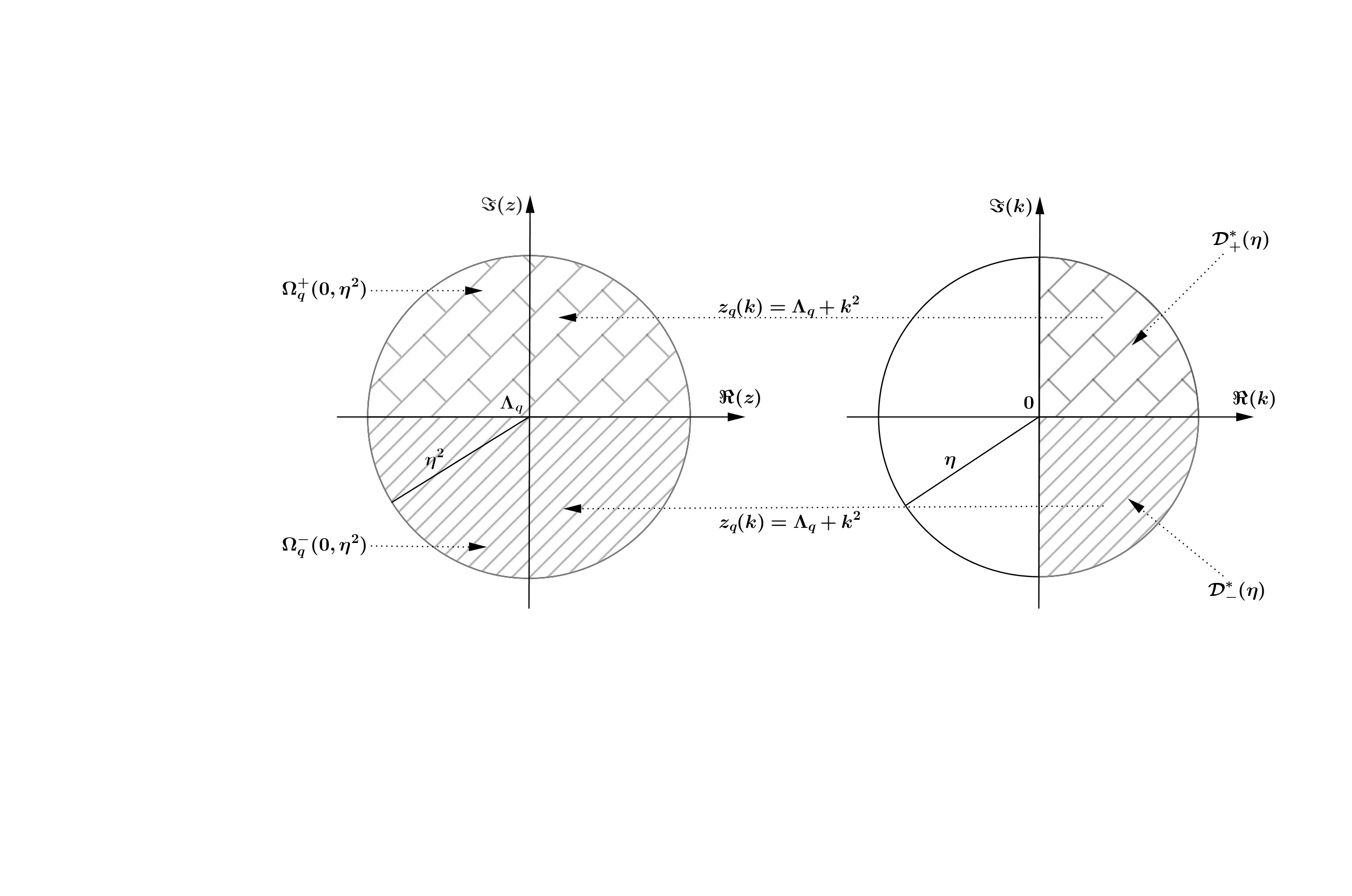
Figure 3.1. Images $\Omega_{q}^{\pm}(0,\eta^{2})$ of $\mathcal{D}_{\pm}^{\ast}(\eta)$ by the local parametrisation $z_{q}(k)=\Lambda_{q}+k^{2}$.

In this subsection, we show how we can reduce the investigation of the discrete eigenvalues $z_{q}(k):=\Lambda_{q}+k^{2}\in\Omega_{q}^{\pm}(0,\eta^{2})$, $k\in\mathcal{D}_{\pm}^{\ast}(\eta)$, to that of the zeros of a holomorphic function on $\Omega_{q}^{\pm}(0,\eta^{2})$.

Let us recall that $P_{q}$, $q\in{\mathbb{N}}$, is the projection onto ${\rm Ker}(H_{\text{Landau}}-\Lambda_{q})$. Hence, introduce in $L^{2}({\mathbb{R}}^{3})$ the projection $p_{q}:=P_{q}\otimes I_{3}$, $q\in{\mathbb{N}}$. With respect to the polar decomposition of $W$, write $W=\tilde{J}|W|$. Then, for any $z\in{\mathbb{C}}\setminus[0,+\infty)$, we have

(3.13) $$\begin{split}&\tilde{J}|W|^{\frac{1}{2}}({H_{0}}-z)^{-1}|W|^{\frac{1}{2}}\\ &=\tilde{J}|W|^{\frac{1}{2}}p_{q}({H_{0}}-z)^{-1}|W|^{\frac{1}{2}}+\sum_{j\neq q}\tilde{J}|W|^{\frac{1}{2}}p_{j}({H_{0}}-z)^{-1}|W|^{\frac{1}{2}}.\end{split}$$

Since

$$(H_{0}-z)^{-1}=\sum_{q\in\mathbb{N}}P_{q}\otimes(D_{x_{3}}^{2}+\Lambda_{q}-z)^{-1},\qquad D_{x_{3}}^{2}:=-\frac{\partial^{2}}{\partial x_{3}^{2}},$$

then for $z=z_{q}(k)$, $k\in\mathcal{D}_{\pm}^{\ast}(\eta)$, the identity (3.13) becomes

(3.14) $$\begin{split}&\tilde{J}|W|^{\frac{1}{2}}\big{(}{H_{0}}-z_{q}(k)\big{)}^{-1}|W|^{\frac{1}{2}}\\ &=\tilde{J}|W|^{\frac{1}{2}}p_{q}(D_{x_{3}}^{2}-k^{2})^{-1}|W|^{\frac{1}{2}}+\sum_{j\neq q}\tilde{J}|W|^{\frac{1}{2}}p_{j}(D_{x_{3}}^{2}+\Lambda_{j}-\Lambda_{q}-k^{2})^{-1}|W|^{\frac{1}{2}}.\end{split}$$

Hence, thanks to Lemma 3.1, we have the following

Proposition 3.1.

Suppose that Assumption (A1) holds. Then, the operator-valued functions

$$\mathcal{D}_{\pm}^{\ast}(\eta)\ni k\longmapsto\mathcal{T}_{W}\big{(}z_{q}(k)\big{)}:=\tilde{J}|W|^{\frac{1}{2}}\big{(}{H_{0}}-z_{q}(k)\big{)}^{-1}|W|^{\frac{1}{2}}$$

are analytic with values in ${\mathcal{S}_{p}}$.

For $z\in{\mathbb{C}}\setminus[0,+\infty)$, on account of Lemma 3.1 and Subsection 3.1, we can introduce the $p$-regularized determinant $\textup{det}_{\lceil p\rceil}\left(I+W({H_{0}}-z)^{-1}\right).$ The following characterization on the discrete eigenvalues is well known $\big{(}$see for instance [37, Chap. 9]$\big{)}$:

(3.15) $$z\in\sigma_{\textup{{disc}}}({H})\Leftrightarrow f(z):=\textup{det}_{\lceil p\rceil}\big{(}I+W({H_{0}}-z)^{-1}\big{)}=0,$$

${H}$ being the perturbed operator defined by (1.9). According to Property d) of Subsection 3.1, if $W({H_{0}}-\cdot)^{-1}$ is holomorphic on a domain $\Omega$, then so is the function $f$ on $\Omega$. Moreover, the algebraic multiplicity of $z\in\sigma_{\textup{{disc}}}({H})$ is equal to its order as zero of the function $f$.

In the next lemma, the notation $Ind_{\gamma}(\cdot)$ in the right hand-side of (3.16) is recalled in the Appendix.

Proposition 3.2.

Let $\mathcal{T}_{W}\big{(}z_{q}(k)\big{)}$ be defined by Proposition 3.1, $k\in\mathcal{D}_{\pm}^{\ast}(\eta)$. Then, the following assertions are equivalent:

(i) $z_{q}(k_{0}):=\Lambda_{q}+k_{0}^{2}\in\Omega_{q}^{\pm}(0,\eta^{2})$ is a discrete eigenvalue of ${H}$,

(ii) $\textup{det}_{\lceil p\rceil}\big{(}I+\mathcal{T}_{W}\big{(}z_{q}(k_{0})\big{)}\big{)}=0$,

(iii) $-1$ is an eigenvalue of $\mathcal{T}_{W}\big{(}z_{q}(k_{0})\big{)}$.
Moreover,

(3.16) $$\textup{mult}\big{(}z_{q}(k_{0})\big{)}=Ind_{\gamma}\hskip 1.42262pt\Big{(}I+\mathcal{T}_{W}\big{(}z_{q}(\cdot)\big{)}\Big{)},$$

$\gamma$ being a small contour positively oriented, containing $k_{0}$ as the unique point $k\in\mathcal{D}_{\pm}^{\ast}(\eta)$ verifying $z_{q}(k)\in\Omega_{q}^{\pm}(0,\eta^{2})$ is a discrete eigenvalue of ${H}$.

Proof.

The equivalence (i) $\Leftrightarrow$ (ii) is an immediate consequence of the characterization (3.15), and the equality

$$\textup{det}_{\lceil p\rceil}\big{(}I+W({H_{0}}-z)^{-1}\big{)}=\textup{det}_{\lceil p\rceil}\big{(}I+\tilde{J}|W|^{\frac{1}{2}}({H_{0}}-z)^{-1}|W|^{\frac{1}{2}}\big{)}.$$

The equivalence (ii) $\Leftrightarrow$ (iii) is an obvious consequence of Property c) of Subsection 3.1.

Now, let us prove the equality (3.16). Consider $f$ the function introduced in (3.15). Thanks to the discussion just after (3.15), if $\gamma^{\prime}$ is a small contour positively oriented containing $z_{q}(k_{0})$ as the unique discrete eigenvalue of ${H}$, then

(3.17) $$\textup{mult}\big{(}z_{q}(k_{0})\big{)}=ind_{\gamma^{\prime}}f.$$

The right hand-side of (3.17) being the index defined by (9.1) of the holomorphic function $f$ with respect to the contour $\gamma^{\prime}$. Then, the equality (3.16) follows directly from the equality

$$ind_{\gamma^{\prime}}f=Ind_{\gamma}\hskip 1.42262pt\Big{(}I+\mathcal{T}_{W}\big{(}z_{q}(\cdot)\big{)}\Big{)},$$

see for instance [3, (2.6)] for more details. This completes the proof. ∎

4. Decomposition of the sandwiched resolvent

We decompose the operator $\mathcal{T}_{W}\big{(}z_{q}(k)\big{)}$, $k\in\mathcal{D}_{\pm}^{\ast}(\eta)$, into a singular part at zero (corresponding to the singularity at the Landau level $\Lambda_{q}=2bq$), and a holomorphic part in $\mathcal{D}_{\pm}^{\ast}(\eta)$, continuous on $\overline{\mathcal{D}_{\pm}^{\ast}(\eta)}$ with values in ${\mathcal{S}_{p}}$.

First, note that due to our choice of the complex square root (3.11), we respectively have $\sqrt{k^{2}}=\pm k$ for $k\in\mathcal{D}_{\pm}^{\ast}(\eta)$.

By (3.14), we have

(4.1) $$\mathcal{T}_{W}\big{(}z_{q}(k)\big{)}=\tilde{J}|W|^{\frac{1}{2}}p_{q}(D_{x_{3}}^{2}-k^{2})^{-1}|W|^{\frac{1}{2}}+\sum_{j\neq q}\tilde{J}|W|^{\frac{1}{2}}p_{j}(D_{x_{3}}^{2}+\Lambda_{j}-\Lambda_{q}-k^{2})^{-1}|W|^{\frac{1}{2}}.$$

Introduce $G_{\pm}$ the multiplication operators by the functions $G^{\pm\frac{1}{2}}(\cdot)$ respectively. Then, we have

(4.2) $$\tilde{J}|W|^{\frac{1}{2}}p_{q}(D_{x_{3}}^{2}-k^{2})^{-1}|W|^{\frac{1}{2}}=\tilde{J}|W|^{\frac{1}{2}}G_{-}P_{q}\otimes G_{+}(D_{x_{3}}^{2}-k^{2})^{-1}G_{+}G_{-}|W|^{\frac{1}{2}}.$$

It follows from the integral kernel

(4.3) $$I_{z}(x_{3},x_{3}^{\prime}):=-\frac{e^{i\sqrt{z}|x_{3}-x_{3}^{\prime}|}}{2i\sqrt{z}}$$

of $(D_{x_{3}}^{2}-z)^{-1}$, $\Im\big{(}\sqrt{z}\big{)}>0$, that $G_{+}(D_{x_{3}}^{2}-k^{2})^{-1}G_{+}$ admits the integral kernel

(4.4) $$\pm G^{\frac{1}{2}}(x_{3})\frac{i\textup{e}^{\pm ik|x_{3}-x_{3}^{\prime}|}}{2k}G^{\frac{1}{2}}(x_{3}^{\prime}),\quad k\in\mathcal{D}_{\pm}^{\ast}(\eta).$$

Then, $G_{+}(D_{x_{3}}^{2}-k^{2})^{-1}G_{+}$ can be decomposed as

(4.5) $$G_{+}(D_{x_{3}}^{2}-k^{2})^{-1}G_{+}=\pm\frac{1}{k}a+b(k),\quad k\in\mathcal{D}_{\pm}^{\ast}(\eta),$$

where $a:L^{2}(\mathbb{R})\longrightarrow L^{2}(\mathbb{R})$ is the rank-one operator defined by

(4.6) $$a(u):=\frac{i}{2}\big{\langle}u,G_{+}\big{\rangle}G_{+},$$

and $b(k)$ the operator with integral kernel

(4.7) $$\pm G^{\frac{1}{2}}(x_{3})i\frac{\textup{e}^{\pm ik|x_{3}-x_{3}^{\prime}|}-1}{2k}G^{\frac{1}{2}}(x_{3}^{\prime}).$$

It can be easily remarked that $-2ia=c^{\ast}c$, where $c:L^{2}(\mathbb{R})\longrightarrow\mathbb{C}$ is the operator defined by $c(u):=\langle u,G_{+}\rangle$, so that $c^{\ast}:\mathbb{C}\longrightarrow L^{2}(\mathbb{R})$ is given by $c^{\ast}(\lambda)=\lambda G_{+}$. This together with (4.5), (4.6), and (4.7), give for any $q\in{\mathbb{N}}$,

(4.8) $$P_{q}\otimes G_{+}(D_{x_{3}}^{2}-k^{2})^{-1}G_{+}=\pm\frac{i}{2k}P_{q}\otimes c^{\ast}c+P_{q}\otimes s(k),\quad k\in\mathcal{D}_{\pm}^{\ast}(\eta),$$

where $s(k)$ is the operator acting from $G^{\frac{1}{2}}(x_{3})L^{2}(\mathbb{R})$ to $G^{-\frac{1}{2}}(x_{3})L^{2}(\mathbb{R})$ with integral kernel given by

(4.9) $$\pm\frac{1-\textup{e}^{\pm ik|x_{3}-x_{3}^{\prime}|}}{2ik}.$$

By combining (4.2) and (4.8), we get for any $k\in\mathcal{D}_{\pm}^{\ast}(\eta)$

(4.10) $$\begin{split}&\tilde{J}|W|^{\frac{1}{2}}p_{q}(D_{x_{3}}^{2}-k^{2})^{-1}|W|^{\frac{1}{2}}\\ &=\pm\frac{i\tilde{J}}{2k}|W|^{\frac{1}{2}}G_{-}(P_{q}\otimes c^{\ast}c)G_{-}|W|^{\frac{1}{2}}+\tilde{J}|W|^{\frac{1}{2}}G_{-}P_{q}\otimes s(k)G_{-}|W|^{\frac{1}{2}}.\end{split}$$

The operator $P_{q}$ admits an explicit integral kernel

(4.11) $$\small{{\mathcal{P}}_{q,b}(X_{\perp},X_{\perp}^{\prime})=\frac{b}{2\pi}L_{q}\left(\frac{b|X_{\perp}-X_{\perp}^{\prime}|^{2}}{2}\right)\exp\Big{(}-\frac{b}{4}\big{(}|X_{\perp}-X_{\perp}^{\prime}|^{2}+2i(x_{1}x_{2}^{\prime}-x_{1}^{\prime}x_{2})\big{)}\Big{)}},$$

where $X_{\perp}=(x_{1},x_{2}),X_{\perp}^{\prime}=(x_{1}^{\prime},x_{2}^{\prime})\in{\mathbb{R}}^{2}$, and $L_{q}(t):=\frac{1}{q!}e^{t}\frac{d^{q}(t^{q}e^{-t})}{dt^{q}}$ are the Laguerre polynomials. Then, (4.10) becomes for any $k\in\mathcal{D}_{\pm}^{\ast}(\eta)$

(4.12) $$\tilde{J}|W|^{\frac{1}{2}}p_{q}(D_{x_{3}}^{2}-k^{2})^{-1}|W|^{\frac{1}{2}}=\pm\frac{i\tilde{J}}{k}K^{\ast}K+\tilde{J}|W|^{\frac{1}{2}}G_{-}P_{q}\otimes s(k)G_{-}|W|^{\frac{1}{2}},$$

where the operator $K$ is given by

(4.13) $$K:=\frac{1}{\sqrt{2}}(P_{q}\otimes c)G_{-}|W|^{\frac{1}{2}}.$$

To be more explicit, the operator $K:L^{2}({\mathbb{R}}^{3})\longrightarrow L^{2}({\mathbb{R}}^{2})$ verifies

$$(K\psi)(X_{\perp})=\frac{1}{\sqrt{2}}\int_{{\mathbb{R}}^{3}}{\mathcal{P}}_{q,b}(X_{\perp},X_{\perp}^{\prime})|W|^{\frac{1}{2}}(X_{\perp}^{\prime},x_{3}^{\prime})\psi(X_{\perp}^{\prime},x_{3}^{\prime})dX_{\perp}^{\prime}dx_{3}^{\prime},$$

${\mathcal{P}}_{q,b}(\cdot,\cdot)$ being the integral kernel given by (4.11), while the adjoint operator $K^{\ast}:L^{2}({\mathbb{R}}^{2})\longrightarrow L^{2}({\mathbb{R}}^{3})$ satisfies

$$(K^{\ast}\varphi)(X_{\perp},x_{3})=\frac{1}{\sqrt{2}}|W|^{\frac{1}{2}}(X_{\perp},x_{3})(P_{q}\varphi)(X_{\perp}).$$

It is easy to check that $KK^{\ast}:L^{2}({\mathbb{R}}^{2})\longrightarrow L^{2}({\mathbb{R}}^{2})$ verifies

(4.14) $$KK^{\ast}=P_{q}\textbf{{W}}P_{q},$$

where W is the multiplication operator by the function W defined by (2.1).

For $\lambda\in{\mathbb{R}}\setminus\{0\}$, define $(D_{x_{3}}^{2}-\lambda)^{-1}$ as the operator with integral kernel

(4.15) $$I_{\lambda}(x_{3},x_{3}^{\prime}):=\lim_{\delta\downarrow 0}I_{\lambda+i\delta}(x_{3},x_{3}^{\prime})=\left\{\begin{array}[]{ccc}\frac{e^{-\sqrt{-\lambda}|x_{3}-x_{3}^{\prime}|}}{2\sqrt{-\lambda}}&\hbox{ if }&\lambda<0,\\ -\frac{e^{i\sqrt{\lambda}|x_{3}-x_{3}^{\prime}|}}{2i\sqrt{\lambda}}&\hbox{ if }&\lambda>0,\end{array}\right.$$

where $I_{z}(\cdot)$ is the integral kernel defined by (4.3). For $0\leq|\lambda|<\sqrt{2b}$, we have

(4.16) $$\begin{split}\Big{\|}\sum_{j\neq q}\tilde{J}|W|^{\frac{1}{2}}&p_{j}(D_{x_{3}}^{2}+\Lambda_{j}-\Lambda_{q}-\lambda^{2})^{-1}|W|^{\frac{1}{2}}\Big{\|}_{\mathcal{S}_{2}}\\ \leq\sum_{j<q}&\Big{\|}\tilde{J}|W|^{\frac{1}{2}}p_{j}(D_{x_{3}}^{2}+\Lambda_{j}-\Lambda_{q}-\lambda^{2})^{-1}|W|^{\frac{1}{2}}\Big{\|}_{\mathcal{S}_{2}}\\ &+\Big{\|}\sum_{j>q}\tilde{J}|W|^{\frac{1}{2}}p_{j}(D_{x_{3}}^{2}+\Lambda_{j}-\Lambda_{q}-\lambda^{2})^{-1}|W|^{\frac{1}{2}}\Big{\|}_{\mathcal{S}_{2}}.\end{split}$$

Since $P_{j}P_{\ell}=\delta_{j,\ell}P_{j}$, then

(4.17) $$\begin{split}\Big{\|}\sum_{j>q}\tilde{J}&|W|^{\frac{1}{2}}p_{j}(D_{x_{3}}^{2}+\Lambda_{j}-\Lambda_{q}-\lambda^{2})^{-1}|W|^{\frac{1}{2}}\Big{\|}^{2}_{\mathcal{S}_{2}}\\ &\leq\text{Const.}\sum_{j>q}\Big{\|}G_{+}(D_{x_{3}}^{2}+\Lambda_{j}-\Lambda_{q}-\lambda^{2})^{-1}G_{+}\Big{\|}^{2}_{\mathcal{S}_{2}}.\end{split}$$

Using the integral kernel (4.15), we obtain

(4.18) $$\left\{\begin{array}[]{ccc}\left\|G_{+}(D_{x_{3}}^{2}+\Lambda_{j}-\Lambda_{q}-\lambda^{2})^{-1}G_{+}\right\|_{\mathcal{S}_{2}}=\mathcal{O}\Big{(}\big{|}2b(q-j)+\lambda^{2}\big{|}^{-\frac{1}{2}}\Big{)}&\hbox{ if }&j<q,\\ \left\|G_{+}(D_{x_{3}}^{2}+\Lambda_{j}-\Lambda_{q}-\lambda^{2})^{-1}G_{+}\right\|^{2}_{\mathcal{S}_{2}}=\mathcal{O}\Big{(}\big{|}2b(q-j)+\lambda^{2}\big{|}^{-\frac{3}{2}}\Big{)}&\hbox{ if }&j>q.\end{array}\right.$$

This together with (4.17) imply that the left hand-side of (4.16) is convergent in ${\mathcal{S}_{2}}$. Moreover, arguing as in [13, Proofs of Propositions 2.1-2.2], it can be shown that $\overline{\mathcal{D}_{\pm}^{\ast}(\eta)}\ni k\mapsto\sum_{j\neq q}\tilde{J}|W|^{\frac{1}{2}}p_{j}(D_{x_{3}}^{2}+\Lambda_{j}-\Lambda_{q}-k^{2})^{-1}|W|^{\frac{1}{2}}\in{\mathcal{S}_{2}}\big{(}L^{2}({\mathbb{R}})\big{)}$ is well defined and continuous. Similarly, as in [6, Subsection 4.1], it can be checked that $\overline{\mathcal{D}_{\pm}^{\ast}(\eta)}\ni k\mapsto G_{+}s(k)G_{+}\in{\mathcal{S}_{2}}\big{(}L^{2}({\mathbb{R}})\big{)}$ is well defined and continuous. Therefore, the following proposition holds:

Proposition 4.1.

Assume that Assumption (A1) holds. Then, for $k\in\mathcal{D}_{\pm}^{\ast}(\eta)$,

(4.19) $$\mathcal{T}_{W}\big{(}z_{q}(k)\big{)}=\pm\frac{i\tilde{J}}{k}\mathscr{B}_{q}+\mathscr{A}_{q}(k),\quad\mathscr{B}_{q}:=K^{\ast}K,$$

where $\tilde{J}$ is defined by the polar decomposition $W=\tilde{J}|W|$. The operator $\mathscr{A}_{q}(k)\in{\mathcal{S}_{p}}$ given by

$$\mathscr{A}_{q}(k):=\tilde{J}|W|^{\frac{1}{2}} G_{-}P_{q}\otimes s(k)G_{-}|W|^{\frac{1}{2}}$$

$$+\sum_{j\neq q}\tilde{J}|W|^{\frac{1}{2}}p_{j}(D_{x_{3}}^{2}+\Lambda_{j}-\Lambda_{q}-k^{2})^{-1}|W|^{\frac{1}{2}}$$

is holomorphic on $\mathcal{D}_{\pm}^{\ast}(\eta)$ and continuous on $\overline{\mathcal{D}_{\pm}^{\ast}(\eta)}$, $s(k)$ being defined by (4.8).

Remark 4.1.

(i) For any $r>0$, we have

(4.20) $$\textup{Tr}\hskip 1.13809pt{\bf 1}_{(r,\infty)}\left(K^{\ast}K\right)=\textup{Tr}\hskip 1.13809pt{\bf 1}_{(r,\infty)}\left(KK^{\ast}\right)=\textup{Tr}\hskip 1.13809pt{\bf 1}_{(r,\infty)}\big{(}P_{q}\textbf{{W}}P_{q}\big{)}.$$

(ii) If $W$ satisfies Assumption (A2) given by (2.10), then Proposition 4.1 holds with $\tilde{J}$ replaced by $Je^{i\alpha}$, where $J=sign(V)$.

5. Proof of Theorem 2.1: Upper bound, general case of electric potentials

The proof falls into two parts.

5.1. A preliminary Proposition

We begin by introducing the numerical range of ${H}$

$$N({H}):=\big{\{}\langle{H}f,f\rangle:f\in Dom({H}),\|f\|_{L^{2}}=1\big{\}}.$$

It is well known (see for instance [8, Lemma 9.3.14]) that $\sigma({H})\subseteq\overline{N({H})}$.

Proposition 5.1.

Fix a Landau level $\Lambda_{q}:=2bq$, $q\in{\mathbb{N}}$. Let $0<s_{0}<\eta$ be sufficiently small. For any $k\in\{0<s<|k|<s_{0}\}\cap\mathcal{D}_{\pm}^{\ast}(\eta)$,

(i) $z_{q}(k):=\Lambda_{q}+k^{2}$ is a discrete eigenvalue of ${H}$ near $\Lambda_{q}$ if and only if $k$ is a zero of

(5.1) $$\mathscr{D}(k,s):=\det\big{(}I+\mathscr{K}(k,s)\big{)}.$$

Here, $\mathscr{K}(k,s)$ is a finite-rank operator analytic with respect to $k$ verifying

$$\small{\textup{rank}\hskip 1.70717pt\mathscr{K}(k,s)=\mathcal{O}\Big{(}\textup{Tr}\hskip 1.13809pt{\bf 1}_{(s,\infty)}\big{(}P_{q}\textbf{{W}}P_{q}\big{)}+1\Big{)},}$$

and $\left\|\mathscr{K}(k,s)\right\|=\mathcal{O}\left(s^{-1}\right)$ uniformly with respect to $s<|k|<s_{0}$.

(ii) Further, if $z_{q}(k_{0}):=\Lambda_{q}+k_{0}^{2}$ is a discrete eigenvalue of ${H}$ near $\Lambda_{q}$, then

(5.2) $$\textup{mult}\big{(}z_{q}(k_{0})\big{)}=Ind_{\gamma}\hskip 1.42262pt\left(I+\mathscr{K}(\cdot,s)\right)=\textup{m}(k_{0}),$$

$\gamma$ being chosen as in (3.16) and $\textup{m}(k_{0})$ being the multiplicity of $k_{0}$ as zero of $\mathscr{D}(k,s)$.

(iii) If $z_{q}(k)$ verifies $\textup{dist}\big{(}z_{q}(k),\overline{N({H})}\big{)}>\varsigma>0$, $\varsigma=\mathcal{O}(1)$, then $I+\mathscr{K}(k,s)$ is invertible and verifies $\left\|\big{(}I+\mathscr{K}(k,s)\big{)}^{-1}\right\|=\mathcal{O}\left(\varsigma^{-1}\right)$ uniformly with respect to $s<|k|<s_{0}$.

Proof.

(i)-(ii) Thanks to Proposition 4.1, $k\mapsto\mathscr{A}_{q}(k)\in{\mathcal{S}_{p}}$ is continuous near zero. Thus, for $s_{0}$ sufficiently small, there exists a finite-rank operator $\mathscr{A}_{0}$ independent of $k$ and $\tilde{\mathscr{A}}(k)\in{\mathcal{S}_{p}}$ continuous near zero, such that $\|\tilde{\mathscr{A}}(k)\|<\frac{1}{4}$, $|k|\leq s_{0}$, with

$$\mathscr{A}_{q}(k)=\mathscr{A}_{0}+\tilde{\mathscr{A}}(k).$$

Decompose $\mathscr{B}_{q}$ defined by (4.19) as

(5.3) $$\mathscr{B}_{q}=\mathscr{B}_{q}{\bf 1}_{[0,\frac{1}{2}s]}(\mathscr{B}_{q})+\mathscr{B}_{q}{\bf 1}_{]\frac{1}{2}s,\infty)}(\mathscr{B}_{q}).$$

We have $\left\|\pm\frac{i\tilde{J}}{k}\mathscr{B}_{q}{\bf 1}_{[0,\frac{1}{2}s]}(\mathscr{B}_{q})+\tilde{\mathscr{A}}(k)\right\|<\frac{3}{4}$ for $0<s<|k|<s_{0}$ so that

(5.4) $$\small{\Big{(}I+\mathcal{T}_{W}\big{(}z_{q}(k)\big{)}\Big{)}=\big{(}I+\mathscr{K}(k,s)\big{)}\left(I\pm\frac{i\tilde{J}}{k}\mathscr{B}_{q}{\bf 1}_{[0,\frac{1}{2}s]}(\mathscr{B}_{q})+\tilde{\mathscr{A}}(k)\right)},$$

$\mathscr{K}(k,s)$ being given by

$$\small{\mathscr{K}(k,s):=\left(\pm\frac{i\tilde{J}}{k}\mathscr{B}_{q}{\bf 1}_{]\frac{1}{2}s,\infty)}(\mathscr{B}_{q})+\mathscr{A}_{0}\right)\left(I\pm\frac{i\tilde{J}}{k}\mathscr{B}_{q}{\bf 1}_{[0,\frac{1}{2}s]}(\mathscr{B}_{q})+\tilde{\mathscr{A}}(k)\right)^{-1}}.$$

Note that $\mathscr{K}(k,s)$ is a finite-rank operator. Moreover, thanks to (4.20), its rank is of order

$$\small{\mathcal{O}\Big{(}\textup{Tr}\hskip 1.13809pt{\bf 1}_{(\frac{1}{2}s,\infty)}(\mathscr{B}_{q})+1\Big{)}=\mathcal{O}\Big{(}\textup{Tr}\hskip 1.13809pt{\bf 1}_{(s,\infty)}\big{(}P_{q}\textbf{{W}}P_{q}\big{)}+1\Big{)}}.$$

It is obvious that its norm is of order $\mathcal{O}\big{(}|k|^{-1}\big{)}=\mathcal{O}\big{(}s^{-1}\big{)}$. Since $\|\pm\frac{i\tilde{J}}{k}\mathscr{B}_{q}{\bf 1}_{[0,\frac{1}{2}s]}(\mathscr{B}_{q})+\tilde{\mathscr{A}}(k)\|<1$ for $0<s<|k|<s_{0}$, then

$$\small{Ind_{\gamma}\hskip 1.42262pt\left(I\pm\frac{i\tilde{J}}{k}\mathscr{B}_{q}{\bf 1}_{[0,\frac{1}{2}s]}(\mathscr{B}_{q})+\tilde{\mathscr{A}}(k)\right)=0}$$

by [18, Theorem 4.4.3]. Hence, (5.2) follows by applying to (5.4) the properties of the index of a finite meromorphic operator-valued function given in the Appendix. Thus, Proposition 3.2 together with (5.2) show that $z_{q}(k)$ is a discrete eigenvalue of ${H}$ if and only if $k$ is a zero of the determinant $\mathscr{D}(k,s)$ defined by (5.1).

(iii) Thanks to (5.4), for $0<s<|k|<s_{0}$, we have

(5.5) $$\small{I+\mathscr{K}(k,s)=\Big{(}I+\mathcal{T}_{W}\big{(}z_{q}(k)\big{)}\Big{)}\left(I+\frac{\tilde{J}}{k}\mathscr{B}_{q}{\bf 1}_{[0,\frac{1}{2}s]}(\mathscr{B}_{q})+\tilde{\mathscr{A}}(k)\right)^{-1}}.$$

It is easy to check from the resolvent equation that

$$\small{\left(I+\tilde{J}|W|^{1/2}({H_{0}}-z)^{-1}|W|^{1/2}\right)\left(I-\tilde{J}|W|^{1/2}({H}-z)^{-1}|W|^{1/2}\right)=I}.$$

Thus, if $z_{q}(k)$ belongs to the resolvent set of ${H}$, then

$$\Big{(}I+\mathcal{T}_{W}\big{(}z_{q}(k)\big{)}\Big{)}^{-1}=I-\tilde{J}|W|^{1/2}\big{(}{H}-z_{q}(k)\big{)}^{-1}|W|^{1/2}.$$

Consequently, according to (5.5), the operator $I+\mathscr{K}(k,s)$ is invertible for $0<s<|k|<s_{0}$, and thanks to [8, Lemma 9.3.14], its satisfies for $\textup{dist}\big{(}z_{q}(k),\overline{N({H})}\big{)}>\varsigma>0$, $\varsigma=\mathcal{O}(1)$,

$$\left\|\big{(}I+\mathscr{K}(k,s)\big{)}^{-1}\right\| =\mathcal{O}\Big{(}1+\left\||W|^{1/2}\big{(}{H}-z_{q}(k)\big{)}^{-1}|W|^{1/2}\right\|\Big{)}$$

$$=\mathcal{O}\big{(}1+\textup{dist}\big{(}z_{q}(k),\overline{N({H})}\big{)}^{-1}\big{)}$$

$$=\mathcal{O}\left(\varsigma^{-1}\right).$$

This concludes the proof. ∎

5.2. Back to the proof of Theorem 2.1

Thanks to Proposition 5.1, for any $0<s<|k|<s_{0}$,

(5.6) $$\mathscr{D}(k,s) =\prod_{j=1}^{\mathcal{O}\big{(}\textup{Tr}\hskip 1.13809pt{\bf 1}_{(s,\infty)}(P_{q}\textbf{{W}}P_{q})+1\big{)}}\big{(}1+\lambda_{j}(k,s)\big{)}$$

$$=\mathcal{O}(1)\hskip 1.42262pt\textup{exp}\hskip 1.42262pt\Big{(}\mathcal{O}\big{(}\textup{Tr}\hskip 1.13809pt{\bf 1}_{(s,\infty)}\big{(}P_{q}\textbf{{W}}P_{q}\big{)}+1\big{)}|\ln s|\Big{)},$$

where the $\lambda_{j}(k,s)$ are the eigenvalues of the operator $\mathscr{K}:=\mathscr{K}(k,s)$ verifying $|\lambda_{j}(k,s)|=\mathcal{O}\left(s^{-1}\right)$. Consider $z_{q}(k)$ satisfying $\textup{dist}\big{(}z_{q}(k),\overline{N({H})}\big{)}>\varsigma>0$ and $0<s<|k|<s_{0}$. We have

$$\mathscr{D}(k,s)^{-1}=\det\big{(}I+\mathscr{K}\big{)}^{-1}=\det\big{(}I-\mathscr{K}(I+\mathscr{K})^{-1}\big{)},$$

and as in (5.6), we can show that

(5.7) $$\small{|\mathscr{D}(k,s)|\geq C\hskip 1.42262pt\textup{exp}\hskip 1.42262pt\Big{(}-C\big{(}\textup{Tr}\hskip 1.13809pt{\bf 1}_{(s,\infty)}\big{(}P_{q}\textbf{{W}}P_{q}\big{)}+1\big{)}\big{(}|\textup{ln}\hskip 1.42262pt\varsigma|+|\textup{ln}\hskip 1.42262pts|\big{)}\Big{)}}.$$

In particular, for $s^{2}<\varsigma<4s^{2}$, $0<r\ll 1$, we deduce from (5.7) that

(5.8) $$-\ln\,|\mathscr{D}(k,s)|\leq C\,\textup{Tr}\hskip 1.13809pt{\bf 1}_{(s,\infty)}\big{(}P_{q}\textbf{{W}}P_{q}\big{)}|\textup{ln}\hskip 1.42262pts|+\mathcal{O}(1).$$

Now, consider the domains $\Delta_{\pm}:=k\in\big{\{}r<|k|<2r:|\Re(k)|>\sqrt{\frac{\nu}{2}}:|\Im(k)|>\sqrt{\frac{\nu}{2}}\big{\}}\cap\mathcal{D}_{\pm}^{\ast}(\eta)$ with $0<r<\sqrt{\|W\|_{\infty}}<\sqrt{\frac{5}{2}}r$ and $0<\nu<2r^{2}$. Since the numerical range $N({H})$ the operator ${H}$ is such that

(5.9) $$N({H})\subseteq\big{\{}z\in{\mathbb{C}}:|\Im(z)|\leq\|W\|_{\infty}\big{\}},$$

then we can find some $k_{0}\in\Delta_{\pm}/r$ such that $\textup{dist}\big{(}z_{q}(rk_{0}),\overline{N({H})}\big{)}\geq\varsigma>r^{2}$, $\varsigma<4r^{2}$. Applying the Jensen Lemma 9.1 with the function $g(k):=\mathscr{D}(rk,r)$, $k\in\Delta_{\pm}/r$, together with (5.6) and (5.8), we get immediately Theorem 2.1.

6. Proof of Theorem 2.2: Upper bound, special case of electric potentials

We prove only the case $\alpha=\frac{3\pi}{4}$; the case $\alpha=-\frac{3\pi}{4}$ follows similarly by replacing $k$ by $-k$, according to (ii) of Remark 2.1 together with Remark 3.1 and (ii) of Remark 4.1.

For any $\theta>0$ small enough, set $\delta=\tan(\theta)$. Introduce the sector

(6.1) $$\mathcal{C}_{\delta}:=\big{\{}k\in{\mathbb{C}}:-\delta\Im(k)\leq|\Re(k)|\big{\}}.$$

Let the assumptions of Theorem 2.2 hold. Then, by Remark 4.1, for any $q\in{\mathbb{N}}$,

(6.2) $$\mathcal{T}_{W}\big{(}z_{q}(k)\big{)}=\frac{ie^{i\alpha}}{k}\mathscr{B}_{q}+\mathscr{A}_{q}(k),\qquad k\in\mathcal{D}_{+}^{\ast}(\eta),$$

where $\mathscr{B}_{q}$ is a positive self-adjoint operator which does not depend on $k$, and $\mathscr{A}_{q}(k)\in{\mathcal{S}_{p}}$ is continuous near $k=0$. Denote $r_{+}:=\max(r,0)$. Since $I+\frac{ie^{i\alpha}}{k}\mathscr{B}_{q}=\frac{ie^{i\alpha}}{k}(\mathscr{B}_{q}-ike^{-i\alpha})$, then for $ike^{-i\alpha}\notin\sigma(\mathscr{B}_{q})$, the operator $I+\frac{ie^{i\alpha}}{k}\mathscr{B}_{q}$ is invertible with

(6.3) $$\small{\left\|\left(I+\frac{ie^{i\alpha}}{k}\mathscr{B}_{q}\right)^{-1}\right\|\leq\frac{|k|}{\sqrt{\big{(}\Im(ke^{-i\alpha})\big{)}_{+}^{2}+|\Re(ke^{-i\alpha})|^{2}}}}.$$

Moreover, for $k\in e^{i\alpha}\mathcal{C}_{\delta}$, it can be checked that, uniformly with respect to $k$, $0<|k|<r_{0}$,

(6.4) $$\small{\left\|\left(I+\frac{ie^{i\alpha}}{k}\mathscr{B}_{q}\right)^{-1}\right\|\leq\sqrt{1+\delta^{-2}}}.$$

Then, according to (6.2), we can write

(6.5) $$\small{I+\mathcal{T}_{W}\big{(}z_{q}(k)\big{)}=\big{(}I+A(k)\big{)}\left(I+\frac{ie^{i\alpha}}{k}\mathscr{B}_{q}\right)},$$

where

(6.6) $$\small{A(k):=\mathscr{A}_{q}(k)\left(I+\frac{ie^{i\alpha}}{k}\mathscr{B}_{q}\right)^{-1}}\in{\mathcal{S}_{p}}.$$

An easy computation shows that

$$\mathcal{T}_{W}\big{(}z_{q}(k)\big{)}-A(k)=\big{(}I+A(k)\big{)}\frac{ie^{i\alpha}}{k}\mathscr{B}_{q}\in\mathcal{S}_{1},$$

since $\mathscr{B}_{q}$ is a trace-class operator if the function $F$ in Assumption (A1) satisfies $F\in L^{1}({\mathbb{R}}^{2})$. Then, we get for any $n\in{\mathbb{N}}^{\ast}$

(6.7) $$\small{\mathcal{T}_{W}^{n}-A^{n}=\mathcal{T}_{W}^{n-1}\left(\mathcal{T}_{W}-A\right)+\left(\mathcal{T}_{W}^{n-1}-A^{n-1}\right)A}\in\mathcal{S}_{1},$$

So, by approximating $A(k)$ by a finite rank-operator and using the fact that

$$\small{\textup{det}_{\lceil p\rceil}(I+T)=\textup{det}(I+T)\exp\left(\sum_{n=1}^{\lceil p\rceil-1}\frac{(-1)^{n}\textup{Tr}\hskip 1.13809pt(T^{n})}{n}\right)}$$

for a trace-class operator $T$ (see Property e) of Subsection 3.1 given by (3.3)), it can be shown with the help of (6.5) that

(6.8) $$\begin{split}\small{\textup{det}_{\lceil p\rceil}\big{(}I+}&\small{\mathcal{T}_{W}\big{(}z_{q}(k)\big{)}\big{)}=\textup{det}\left(I+\frac{ie^{i\alpha}}{k}\mathscr{B}_{q}\right)}\\ &\small{\times\textup{det}_{\lceil p\rceil}\big{(}I+A(k)\big{)}\exp\left(\sum_{n=1}^{\lceil p\rceil-1}\frac{(-1)^{n}\textup{Tr}\hskip 1.13809pt\bigl{(}\mathcal{T}_{W}^{n}-A^{n}\bigr{)}}{n}\right)}.\end{split}$$

Thus, for $0<|k|<r_{0}$ small enough, $k\in e^{i\alpha}\mathcal{C}_{\delta}$, the zeros of $\textup{det}_{\lceil p\rceil}\big{(}I+\mathcal{T}_{W}\big{(}z_{q}(k)\big{)}\big{)}$ are those of $\textup{det}_{\lceil p\rceil}\big{(}I+A(k)\big{)}$ with the same multiplicities thanks to Proposition 3.2 and Property (9.3) applied to (6.5).

Since $\mathscr{A}_{q}(\cdot)\in{\mathcal{S}_{p}}$ is continuous near $k=0$, this together with (6.4) implies that the ${\mathcal{S}_{p}}$-norm of $A(k)$ is uniformly bounded with respect to $0<|k|<r_{0}$ small enough, $k\in e^{i\alpha}\mathcal{C}_{\delta}$. Then, thanks to Property f) of Subsection 3.1 given by (3.4), we have

(6.9) $$\small{\textup{det}_{\lceil p\rceil}\big{(}I+A(k)\big{)}=\mathcal{O}\left(e^{\mathcal{O}\big{(}\|A(k)\|_{{\mathcal{S}_{p}}}^{p}\big{)}}\right)=\mathcal{O}(1).}$$

Now, let us establish a lower bound of $\textup{det}_{\lceil p\rceil}\big{(}I+A(k)\big{)}$. Thanks to (6.5), we have

(6.10) $$\small{\big{(}I+A(k)\big{)}^{-1}=\left(I+\frac{ie^{i\alpha}}{k}\mathscr{B}_{q}\right)\big{(}I+\mathcal{T}_{W}\big{(}z_{q}(k)\big{)}^{-1}}.$$

Hence, by reasoning as in the proof of (iii)-Proposition 5.1, we obtain for $0<s<|k|<r_{0}$ and $\textup{dist}\big{(}z_{q}(k),\overline{N({H})}\big{)}>\varsigma>0$, $\varsigma=\mathcal{O}(1)$, uniformly with respect to $(k,s)$,

(6.11) $$\small{\left\|\big{(}I+A(k)\big{)}^{-1}\right\|=\mathcal{O}\big{(}s^{-1}\big{)}\mathcal{O}\big{(}\varsigma^{-1}\big{)}}.$$

Let $(\mu_{j})_{j}$ be the sequence of eigenvalues of $A(k)$. We have

(6.12) $$\small{\left|\big{(}\textup{det}_{\lceil p\rceil}(I+A(k))\big{)}^{-1}\right|} \small{=\left|\textup{det}\left((I+A(k))^{-1}e^{\sum_{n=1}^{\lceil p\rceil-1}\frac{(-1)^{n+1}A(k)^{n}}{n}}\right)\right|}$$

$$\small{\leq\prod_{|\mu_{j}|\leq\frac{1}{2}}\left|\frac{e^{\sum_{n=1}^{\lceil p\rceil-1}\frac{(-1)^{n+1}\mu_{j}^{n}}{n}}}{1+\mu_{j}}\right|\times\prod_{|\mu_{j}|>\frac{1}{2}}\frac{e^{\left|\sum_{n=1}^{\lceil p\rceil-1}\frac{(-1)^{n+1}\mu_{j}^{n}}{n}\right|}}{|1+\mu_{j}|}.}$$

Using the fact that $A(k)$ is uniformly bounded in ${\mathcal{S}_{p}}$ with respect to $0<|k|<r_{0}$ small enough, $k\in e^{i\alpha}\mathcal{C}_{\delta}$, it is easy to check that the first product is uniformly bounded. On the other hand, thanks to (6.11), we have for $0<s<|k|<r_{0}$ and $\textup{dist}\big{(}z_{q}(k),\overline{N({H})}\big{)}>\varsigma>0$, $\varsigma=\mathcal{O}(1)$,

(6.13) $$\small{|1+\mu_{j}|^{-1}=\mathcal{O}\big{(}s^{-1}\big{)}\mathcal{O}\big{(}\varsigma^{-1}\big{)}},$$

uniformly with respect to $k$, $s$. Consequently, since there exists a finite number of terms $\mu_{j}$ lying in the second product, we deduce from (6.12) that

(6.14) $$\small{\left|\textup{det}_{\lceil p\rceil}\big{(}I+A(k)\big{)}\right|\geq Ce^{-C\big{(}|\ln\varsigma|+|\ln s|\big{)}}},$$

for some positive constant $C>0$. Now, one concludes as in the proof of Theorem 2.1 by using the Jensen Lemma 9.1.

7. Theorem 2.3: Lower bound, upper bound and sectors free of complex eigenvalues

As in the previous section, we only prove the case $\alpha\in(0,\pi)$. For $\alpha\in-(0,\pi)$, it suffices to replace $k$ by $-k$.

(i) Under the assumptions of Theorem 2.3, for any $q\in{\mathbb{N}}$, we have

(7.1) $$I+\mathcal{T}_{\varepsilon W}\big{(}z_{q}(k)\big{)}=I+\frac{i\varepsilon e^{i\alpha}}{k}\mathscr{B}_{q}+\varepsilon\mathscr{A}_{q}(k),\qquad k\in\mathcal{D}_{+}^{\ast}(\eta).$$

Similarly to the proof of Theorem 2.2, for $ike^{-i\alpha}\notin\sigma(\varepsilon\mathscr{B}_{q})$, the operator $I+\frac{i\varepsilon e^{i\alpha}}{k}\mathscr{B}_{q}$ is invertible. Further, for $k\in e^{i\alpha}\mathcal{C}_{\delta}$, $\delta=\tan(\theta)$, we have

(7.2) $$\small{\left\|\left(I+\frac{i\varepsilon e^{i\alpha}}{k}\mathscr{B}_{q}\right)^{-1}\right\|\leq\sqrt{1+\delta^{-2}}},$$

uniformly with respect to $k$, $0<|k|<r_{0}$. Then, as in (6.5) and (6.6), we have

(7.3) $$\small{I+\mathcal{T}_{\varepsilon W}\big{(}z_{q}(k)\big{)}=\big{(}I+A(k)\big{)}\left(I+\frac{i\varepsilon e^{i\alpha}}{k}\mathscr{B}_{q}\right)},$$

with

(7.4) $$\small{A(k):=\varepsilon\mathscr{A}_{q}(k)\left(I+\frac{i\varepsilon e^{i\alpha}}{k}\mathscr{B}_{q}\right)^{-1}}\in{\mathcal{S}_{p}}.$$

Since $\mathscr{A}_{q}(\cdot)\in{\mathcal{S}_{p}}$ is continuous near $k=0$, then there exists a constant $C>0$ such that $\|\mathscr{A}_{q}(k)\|\leq C$. This together with (7.2) and (7.4) imply that for $0<\varepsilon<\big{(}C\sqrt{1+\delta^{-2}}\big{)}^{-1}$, the operator $I+\mathcal{T}_{\varepsilon W}\big{(}z_{q}(k)\big{)}$ is invertible for $k\in e^{i\alpha}\mathcal{C}_{\delta}$. Consequently, $z_{q}(k)$ is not a discrete eigenvalue.

(ii) Decompose $\varepsilon\mathscr{B}_{q}$ as $\varepsilon\mathscr{B}_{q}=\mathscr{B}_{+}+\mathscr{B}_{-}$, where $\mathscr{B}_{+}$ and $\mathscr{B}_{-}$ are defined by

(7.5) $$\mathscr{B}_{+}:=\varepsilon\mathscr{B}_{q}{\bf 1}_{[\frac{r}{2},4r]}(\varepsilon\mathscr{B}_{q}),\qquad\mathscr{B}_{-}:=\varepsilon\mathscr{B}_{q}{\bf 1}_{]0,\frac{r}{2}[\cup]4r,\infty[}(\varepsilon\mathscr{B}_{q}).$$

It is easy to verify that for $\frac{2r}{3}<|k|<\frac{3r}{2}$, we have $\sigma\big{(}\frac{1}{|k|}\mathscr{B}_{-}\big{)}\subset\left[0,\frac{3}{4}\right]\cup\left[\frac{8}{3},\infty\right[$. Therefore, $I+\frac{ie^{i\alpha}}{k}\mathscr{B}_{-}$ is invertible with

(7.6) $$\small{\left\|\left(I+\frac{ie^{i\alpha}}{k}\mathscr{B}_{-}\right)^{-1}\right\|\leq 4},$$

uniformly with respect to $0<|k|<r_{0}$. Thus, for $0<\varepsilon\leq\varepsilon_{0}$ small enough, $I+\frac{ie^{i\alpha}}{k}\mathscr{B}_{-}+\varepsilon\mathscr{A}_{q}(k)$ is invertible with a uniformly bounded inverse given by

(7.7) $$\small{\left(I+\frac{ie^{i\alpha}}{k}\mathscr{B}_{-}+\varepsilon\mathscr{A}_{q}(k)\right)^{-1}=\left(I+\frac{ie^{i\alpha}}{k}\mathscr{B}_{-}\right)^{-1}\left(I+\varepsilon\mathscr{A}_{q}(k)\left(I+\frac{ie^{i\alpha}}{k}\mathscr{B}_{-}\right)^{-1}\right)^{-1}.}$$

This together with (7.1) and (7.5) allow to write

(7.8) $$\small{I+\mathcal{T}_{\varepsilon W}\big{(}z_{q}(k)\big{)}=\left(I+\frac{ie^{i\alpha}}{k}\mathscr{B}_{-}+\varepsilon\mathscr{A}_{q}(k)\right)\left(I+\left(I+\frac{ie^{i\alpha}}{k}\mathscr{B}_{-}+\varepsilon\mathscr{A}_{q}(k)\right)^{-1}\frac{ie^{i\alpha}}{k}\mathscr{B}_{+}\right).}$$

Since $I+\frac{ie^{i\alpha}}{k}\mathscr{B}_{-}+\varepsilon\mathscr{A}_{q}(k)$ is invertible and $\mathscr{B}_{+}$ is a trace-class operator, then by exploiting Proposition 3.2 and Property (9.3) applied to (7.8), we see that the discrete eigenvalues of ${H}_{\varepsilon}$ are the zeros of

(7.9) $$\small{\tilde{D}(k,r):=\textup{det}\left(I+\left(I+\frac{ie^{i\alpha}}{k}\mathscr{B}_{-}+\varepsilon\mathscr{A}_{q}(k)\right)^{-1}\frac{ie^{i\alpha}}{k}\mathscr{B}_{+}\right)}$$

with the same multiplicities. Moreover, since $\frac{ie^{i\alpha}}{k}\mathscr{B}_{+}$ is uniformly bounded with $\|\frac{ie^{i\alpha}}{k}\mathscr{B}_{+}\|\leq 6$, then as in (5.6) it can be shown that

(7.10) $$\small{\tilde{D}(k,r)=\exp\left(\mathcal{O}\left(\textup{Tr}\hskip 1.13809pt{\bf 1}_{[\frac{r}{2},4r]}(\varepsilon\mathscr{B}_{q})\right)\right).}$$

Now, establish a lower bound of $\tilde{D}(ik,r)$ for $0<\frac{2r}{3}<|k|<\frac{3r}{2}$, $k\in{\mathbb{R}}_{+}e^{-i\beta}$, $\beta>0$ such that $z_{q}(ik)=2bq-k^{2}\in\Omega_{q,\nu}^{+}\Big{(}\frac{4r^{2}}{9},\frac{9r^{2}}{4}\Big{)}$, $0<\nu<\frac{8r^{2}}{9}$, is not a discrete eigenvalue of $H_{\varepsilon}$. Under this condition, thanks to (7.7) and (7.8), $I+\left(I+\frac{e^{i\alpha}}{k}\mathscr{B}_{-}+\varepsilon\mathscr{A}_{q}(k)\right)^{-1}\frac{e^{i\alpha}}{k}\mathscr{B}_{+}$ is invertible. On the other hand, by exploiting the fact that $\mathscr{B}_{+}\mathscr{B}_{-}=\mathscr{B}_{-}\mathscr{B}_{+}=0$, we get

(7.11) $$\begin{split}\Big{(}I&+\frac{e^{i\alpha}}{k}\mathscr{B}_{-}+\varepsilon\mathscr{A}_{q}(k)\Big{)}^{-1}\frac{e^{i\alpha}}{k}\mathscr{B}_{+}\\ &=\left[I-\left(I+\frac{e^{i\alpha}}{k}\mathscr{B}_{-}+\varepsilon\mathscr{A}_{q}(k)\right)^{-1}\left(\frac{e^{i\alpha}}{k}\mathscr{B}_{-}+\varepsilon\mathscr{A}_{q}(k)\right)\right]\frac{e^{i\alpha}}{k}\mathscr{B}_{+}\\ &=\frac{e^{i\alpha}}{k}\mathscr{B}_{+}+\mathcal{O}(\varepsilon).\end{split}$$

Then, for $f\in L^{2}({\mathbb{R}}^{3})\setminus{\rm Ker}\,(\mathscr{B}_{+})$, we have

(7.12) $$\begin{split}&\Biggl{|}\Im\left(\Big{\langle}\Big{(}I+\frac{e^{i\alpha}}{k}\mathscr{B}_{-}+\varepsilon\mathscr{A}_{q}(k)\Big{)}^{-1}\frac{e^{i\alpha}}{k}\mathscr{B}_{+}f,f\Big{\rangle}\right)\Biggr{|}\\ &=\Biggl{|}\Im\left(\Big{\langle}\Big{(}\frac{e^{i\alpha}}{k}\mathscr{B}_{+}+\mathcal{O}(\varepsilon)\Big{)}f,f\Big{\rangle}\right)\Biggr{|}\\ &=\Bigl{|}\sin(\alpha+\beta)\Big{\langle}\frac{\mathscr{B}_{+}}{|k|}f,f\Big{\rangle}+\Im\left(\Big{\langle}\mathcal{O}(\varepsilon)f,f\Big{\rangle}\right)\Bigr{|}\geq\textup{Const.}\big{|}\sin(\alpha+\beta)\big{|}\|f\|^{2},\end{split}$$

for $\varepsilon$ small enough and using the fact that $\sigma\big{(}\frac{1}{|k|}\mathscr{B}_{+}\big{)}\subset\left]\frac{1}{3},6\right[$. For $f\in{\rm Ker}\,(\mathscr{B}_{+})$, we have

(7.13) $$\Re\left(\Big{\langle}\Big{(}I+\Big{(}I+\frac{e^{i\alpha}}{k}\mathscr{B}_{-}+\varepsilon\mathscr{A}_{q}(k)\Big{)}^{-1}\frac{e^{i\alpha}}{k}\mathscr{B}_{+}\Big{)}f,f\Big{\rangle}\right)=\|f\|^{2}.$$

Thus,

(7.14) $$\left\|\left(I+\left(I+\frac{e^{i\alpha}}{k}\mathscr{B}_{-}+\varepsilon\mathscr{A}_{q}(k)\right)^{-1}\frac{e^{i\alpha}}{k}\mathscr{B}_{+}\right)^{-1}\right\|\leq C(\alpha,\beta),$$

where $C(\alpha,\beta)$ is a constant depending on $\alpha$ and $\beta$. Consequently, as in (7.10), it can be shown that

(7.15) $$\begin{split}\tilde{D}(ik,r)^{-1}=\textup{det}\Big{\{}I-&\Big{(}I+\frac{e^{i\alpha}}{k}\mathscr{B}_{-}+\varepsilon\mathscr{A}_{q}(k)\Big{)}^{-1}\frac{e^{i\alpha}}{k}\mathscr{B}_{+}\\ &\Big{[}I+\Big{(}I+\frac{e^{i\alpha}}{k}\mathscr{B}_{-}+\varepsilon\mathscr{A}_{q}(k)\Big{)}^{-1}\frac{e^{i\alpha}}{k}\mathscr{B}_{+}\Big{]}^{-1}\Big{\}}\\ &\leq\exp\left(\mathcal{O}\left(\textup{Tr}\hskip 1.13809pt{\bf 1}_{[\frac{r}{2},4r]}(\varepsilon\mathscr{B}_{q})\right)\right).\end{split}$$

Namely,

(7.16) $$\small{\tilde{D}(ik,r)\geq\exp\left(-C\left(\textup{Tr}\hskip 1.13809pt{\bf 1}_{[\frac{r}{2},4r]}(\varepsilon\mathscr{B}_{q})\right)\right)},$$

for some constant $C>0$. We conclude as in the proof of Theorem 2.1 by using the Jensen Lemma 9.1.

(iii) Counted with their multiplicity, denote $(\mu_{j})_{j}$ the decreasing sequence of the non-vanishing eigenvalues of the operator $P_{p}\textbf{{W}}P_{q}$. Following [2, Lemma 7], there exits a constant $\nu>0$ such that

(7.17) $$\#\big{\{}j:\mu_{j}-\mu_{j+1}>\nu\mu_{j}\big{\}}=\infty.$$

Since $\mathscr{B}_{q}$ and $P_{p}\textbf{{W}}P_{q}$ have the same non-vanishing eigenvalues, then there exists a decreasing sequence of positive numbers $(r_{\ell})_{\ell}$ with $r_{\ell}\searrow 0$, satisfying for any $\ell\in{\mathbb{N}}$ (see Figure 7.1)

(7.18) $$\textup{dist}\big{(}r_{\ell},\sigma(\mathscr{B}_{q})\big{)}\geq\frac{\nu r_{\ell}}{2}.$$

Moreover, for any $\ell\in{\mathbb{N}}$, there exists a path $\tilde{\Sigma}_{\ell}:=\partial\omega_{\ell}$ (see Figure 7.1) with

(7.19) $$\omega_{\ell}:=\big{\{}\tilde{k}\in{\mathbb{C}}:0<|\tilde{k}|<r_{0}:|\Im(\tilde{k})|\leq\delta\Re(\tilde{k}):r_{\ell+1}\leq\Re(\tilde{k})\leq r_{\ell}\big{\}},$$

enclosing the eigenvalues of the operator $\mathscr{B}_{q}$ contained in $[r_{\ell+1},r_{\ell}]$.

Figure 7.1. Representation of the path $\tilde{\Sigma}_{\ell}=\partial\omega_{\ell}$.

It can be checked that the invertible operator $\tilde{k}-\mathscr{B}_{q}$ for $\tilde{k}\in\tilde{\Sigma}_{\ell}$ satisfies

(7.20) $$\big{\|}(\tilde{k}-\mathscr{B}_{q})^{-1}\big{\|}\leq\frac{\max\left(\delta^{-1}\sqrt{1+\delta^{2}},(\nu/2)^{-1}\sqrt{1+\delta^{2}}\right)}{|\tilde{k}|},$$

uniformly with respect to $\tilde{k}\in\tilde{\Sigma}_{\ell}$. Introduce the path $\Sigma_{\ell}:=-i\varepsilon e^{i\alpha}\tilde{\Sigma}_{\ell}$ and estimate from below the number of zeros of $\textup{det}_{\lceil p\rceil}\big{(}I+\frac{i\varepsilon e^{i\alpha}}{k}\mathscr{B}_{q}+\varepsilon\mathscr{A}_{q}(k)\big{)}$ enclosed in $\big{\{}z_{q}(k)\in\Omega_{q}^{+}(0,\eta^{2}):k\in\omega_{\ell}\big{\}}$, counted with their multiplicity. It is easy to see that according to the construction of $\Sigma_{\ell}$ and (7.20), $I+\frac{i\varepsilon e^{i\alpha}}{k}\mathscr{B}_{q}$ is invertible for $k\in\Sigma_{\ell}$ and satisfies

(7.21) $$\left\|\left(I+\frac{i\varepsilon e^{i\alpha}}{k}\mathscr{B}_{q}\right)^{-1}\right\|\leq\max\left(\delta^{-1}\sqrt{1+\delta^{2}},(\nu/2)^{-1}\sqrt{1+\delta^{2}}\right),$$

uniformly with respect to $k\in\Sigma_{\ell}$. Then, for $k\in\Sigma_{\ell}$,

(7.22) $$\small{I+\frac{i\varepsilon e^{i\alpha}}{k}\mathscr{B}_{q}+\varepsilon\mathscr{A}_{q}(k)=\left(I+\varepsilon\mathscr{A}_{q}(k)\left(I+\frac{i\varepsilon e^{i\alpha}}{k}\mathscr{B}_{q}\right)^{-1}\right)\left(I+\frac{i\varepsilon e^{i\alpha}}{k}\mathscr{B}_{q}\right).}$$

Choosing $0<\varepsilon\leq\varepsilon_{0}$ small enough and using Property g) of Subsection 3.1 given by (3.5), we get for $k\in\Sigma_{\ell}$

(7.23) $$\small{\left|\textup{det}_{\lceil p\rceil}\left[I+\varepsilon\mathscr{A}_{q}(k)\left(I+\frac{i\varepsilon e^{i\alpha}}{k}\mathscr{B}_{q}\right)^{-1}\right]-1\right|<1}.$$

Consequently, by the Rouché Theorem, the number of zeros of $\textup{det}_{\lceil p\rceil}\big{(}I+\frac{i\varepsilon e^{i\alpha}}{k}\mathscr{B}_{q}+\varepsilon\mathscr{A}_{q}(k)\big{)}$ enclosed in $\big{\{}z_{q}(k)\in\Omega_{q}^{+}(0,\eta^{2}):k\in\omega_{\ell}\big{\}}$ counted with their multiplicity, is equal to that of $\textup{det}_{\lceil p\rceil}\big{(}I+\frac{i\varepsilon e^{i\alpha}}{k}\mathscr{B}_{q}\big{)}$ enclosed in $\big{\{}z_{q}(k)\in\Omega_{q}^{+}(0,\eta^{2}):k\in\omega_{\ell}\big{\}}$ counted with their multiplicity. Thanks to (4.20), this number is equal to $\textup{Tr}\hskip 1.13809pt{\bf 1}_{[r_{\ell+1},r_{\ell}]}\big{(}P_{q}\textbf{{W}}P_{q}\big{)}$. So, we get (2.16) since the zeros of $\textup{det}_{\lceil p\rceil}\big{(}I+\frac{i\varepsilon e^{i\alpha}}{k}\mathscr{B}_{q}+\varepsilon\mathscr{A}_{q}(k)\big{)}$ are the discrete eigenvalues of ${H}_{\varepsilon}$ with the same multiplicity, thanks to Proposition 3.2 and Property (9.3) applied to (7.22). The infiniteness of the number of the discrete eigenvalues claimed follows from the fact that the sequence $(r_{\ell})_{\ell}$ is infinite tending to zero. The proof is complete.

8. Proof of Theorem 2.4: Dominated accumulation

The proof goes as that of item (i) of Theorem 2.3.

Let the assumptions of Theorem 2.4 hold. Then, for any $q\in{\mathbb{N}}$, we have

(8.1) $$I+\mathcal{T}_{\varepsilon W}\big{(}z_{q}(k)\big{)}=I\pm\frac{i\varepsilon e^{i\alpha}}{k}\mathscr{B}_{q}+\varepsilon\mathscr{A}_{q}(k),\qquad k\in\mathcal{D}_{\pm}^{\ast}(\eta).$$

The operator $I\pm\frac{i\varepsilon e^{i\alpha}}{k}\mathscr{B}_{q}$ satisfies the bound (7.2) for $k\in e^{i\alpha}\mathcal{C}_{\delta}$, uniformly with respect to $0<|k|<\eta$. Then,

(8.2) $$\small{I+\mathcal{T}_{\varepsilon W}\big{(}z_{q}(k)\big{)}=\big{(}I+A_{\pm}(k)\big{)}\left(I\pm\frac{i\varepsilon e^{i\alpha}}{k}\mathscr{B}_{q}\right)},$$

with

(8.3) $$\small{A_{\pm}(k):=\varepsilon\mathscr{A}_{q}(k)\left(I\pm\frac{i\varepsilon e^{i\alpha}}{k}\mathscr{B}_{q}\right)^{-1}}.$$

From Proposition 4.1, we deduce that there exists a constant $C>0$ such that $\|\mathscr{A}_{q}(k)\|\leq C$ uniformly with respect to $0\leq|k|\leq\eta$. Then, for $0<\varepsilon\leq\tilde{\varepsilon}_{0}$ small enough, $I+\mathcal{T}_{\varepsilon W}\big{(}z_{q}(k)\big{)}$ is invertible for $k\in e^{i\alpha}\mathcal{C}_{\delta}$. Therefore, $z_{q}(k)$ is not a discrete eigenvalue, which proves the theorem.

9. Appendix

In this Appendix, we recall the notion of the index (with respect to a positively oriented contour) of a holomorphic function and a finite meromorphic operator-valued function, see for instance [3, Definition 2.1].

For $f$ a holomorphic function in a neighbourhood of a contour $\gamma$, the index of $f$ with respect to $\gamma$ is defined by

(9.1) $$ind_{\gamma}\hskip 1.42262ptf:=\frac{1}{2i\pi}\int_{\gamma}\frac{f^{\prime}(z)}{f(z)}dz.$$

Noting that if $f$ is holomorphic in a domain $\Omega$ with $\partial\Omega=\gamma$, then the residues theorem implies that $\textup{ind}_{\gamma}\hskip 1.42262ptf$ coincides with the number of zeros of $f$ in $\Omega$, counted with their multiplicity.

Consider $D\subseteq\mathbb{C}$ a connected open set, $Z\subset D$ being a pure point and closed subset, and $A:\overline{D}\backslash Z\longrightarrow\textup{GL}(\mathscr{H})$ (the class of invertible operators on $\mathscr{H}$) being a finite meromorphic operator-valued function and Fredholm at each point of $Z$. The index of $A$ with respect to the contour $\partial\Omega$ is defined by

(9.2) $$\small{Ind_{\partial\Omega}\hskip 1.42262ptA:=\frac{1}{2i\pi}\textup{Tr}\int_{\partial\Omega}A^{\prime}(z)A(z)^{-1}dz=\frac{1}{2i\pi}\textup{Tr}\int_{\partial\Omega}A(z)^{-1}A^{\prime}(z)dz}.$$

We have the following properties:

(9.3) $$Ind_{\partial\Omega}\hskip 1.42262ptA_{1}A_{2}=Ind_{\partial\Omega}\hskip 1.42262ptA_{1}+Ind_{\partial\Omega}\hskip 1.42262ptA_{2},$$

and if $K(z)$ lies in the trace class operator, then

(9.4) $$Ind_{\partial\Omega}\hskip 1.42262pt(I+K)=ind_{\partial\Omega}\hskip 1.42262pt\det\hskip 1.42262pt(I+K).$$

For more details, see [18, Chap. 4].

The following lemma contains a version of the well-known Jensen inequality, see for instance [2, Lemma 6] for a proof.

Lemma 9.1.

Let $\Delta$ be a simply connected sub-domain of $\mathbb{C}$ and let $g$ be a holomorphic function in $\Delta$ with continuous extension to $\overline{\Delta}$. Assume that there exists $\lambda_{0}\in\Delta$ such that $g(\lambda_{0})\neq 0$ and $g(\lambda)\neq 0$ for $\lambda\in\partial\Delta$, the boundary of $\Delta$. Let $\lambda_{1},\lambda_{2},\ldots,\lambda_{N}\in\Delta$ be the zeros of $g$ repeated according to their multiplicity. For any domain $\Delta^{\prime}\Subset\Delta$, there exists $C^{\prime}>0$ such that $N(\Delta^{\prime},g)$, the number of zeros $\lambda_{j}$ of $g$ contained in $\Delta^{\prime}$, satisfies

(9.5) $$N(\Delta^{\prime},g)\leq C^{\prime}\left(\int_{\partial\Delta}\textup{ln}|g(\lambda)|d\lambda-\textup{ln}|g(\lambda_{0})|\right).$$

References

[1]J. Avron, I. Herbst, B. Simon,
Schrödinger operators with magnetic fields. I. General interactions,
Duke Math. J. 45 (1978), 847-883.
[2]J.-F. Bony, V. Bruneau, G. Raikov,
Resonances and Spectral Shift Function near the Landau levels,
Ann. Inst. Fourier, 57(2) (2007), 629-671.
[3]J.-F. Bony, V. Bruneau, G. Raikov,
Counting function of characteristic values and magnetic resonances,
Commun. PDE. 39 (2014), 274-305.
[4]A. Borichev, L. Golinskii, S. Kupin,
A Blaschke-type condition and its application to complex Jacobi matrices,
Bull. London Math. Soc. 41 (2009), 117-123.
[5]V. Bruneau, E. M. Ouhabaz,
Lieb-Thirring estimates for non-seladjoint Schrödinger operators,
J. Math. Phys. 49 (2008).
[6]V. Bruneau, A. Pushnitski, G. Raikov,
Spectral shift function in strong magnetic fields,
Algebra in Analiz, 16 (2004), 207-238;
St. Petersburg Math. J. 16 (2005), 181-209.
[7]J.-C Cuenin, A. Laptev, C. Tretter,
Eigenvalues estimates for non-selfadjoint Dirac operators on the real line,
preprint on http://http://arxiv.org/pdf/1207.6584.
[8]E. B. Davies,
Linear Operators and their Spectra,
Camb. Stu. Adv. Math. 106 (2007), Cambridge University Press.
[9]M. Demuth, M. Hansmann, G. Katriel,
On the discrete spectrum of non-seladjoint operators,
J. Funct. Anal. 257(9) (2009), 2742-2759.
[10]M. Demuth, M. Hansmann, G. Katriel,
Eingenvalues of non-selfadjoint operators: a comparison of two approaches,
Operator Theory: Advances and Applications, 232, 107-163.
[11]M. Dimassi, G. D. Raikov,
Spectral asymptotics for quantum Hamiltonians in strong magnetic fields,
Cubo Math. Educ 3(2) (2001), 317-391.
[12]C. Dubuisson,
On quantitative bounds on eigenvalues of a complex perturbation of a Dirac operator,
Int. Eq. Operator Theory 78(2) (2014), 249–269.
[13]C. Fernandez, G. D. Raikov,
On the singularities of the magnetic spectral shift function at the landau levels,
Ann. Henri Poincaré, 5 (2004), no. 2, 381-403.
[14]G. B. Folland,
Real analysis Modern techniques and their applications,
Pure and Apllied Mathematics, (1984), John Whiley and Sons.
[15]R. L. Frank, A. Laptev, E. H. Lieb, R. Seiringer,
Lieb-Thirring inequalities for Schrödinger operators with complex-valued potentials,
Lett. in Math. Phys. 77 (2006), 309-316.
[16]L. Golinskii, S. Kupin,
On discrete spectrum of complex perturbations of finite band Schrödinger operators,
in "Recent trends in Analysis", Proceedings of the conference in honor of N. Nikolski, Université
Bordeaux 1, 2011, Theta Foundation, Bucharest, Romania, 2013.
[17]I. Gohberg, E. I. Sigal,
An operator generalization of the logarithmic residue theorem and Rouché’s theorem,
Mat. Sb. (N.S.) 84 (126) (1971), 607-629.
[18]I. Gohberg, J. Leiterer,
Holomorphic operator functions of one variable and applications,
Operator Theory, Advances and Applications, vol. 192 Birkhäuser Verlag, 2009, Methods
from complex analysis in several variables.
[19]M. Hansmann,
Variation of discrete spectra for non-selfadjoint perturbations of selfadjoint operators,
Int. Eq. Op. Theory, 76(2) (2013) 163-178.
[20]V. Ya. Ivrii,
Microlocal Analysis and Precise Spectral Asymptotics,
Springer-Verlag, Berlin, 1998.
[21]T. Kato,
Perturbation Theory for Linear Operators,
Springer-Verlag, Berlin, 1966.
[22]E. H. Lieb, W. Thirring,
Bound for the kinetic energy of fermions which proves the stability of matter,
Phys. Rev. lett. 35 (1975), 687-689. Errata 35 (1975), 1116.
[23]E. H. Lieb, M. Loss, Analysis, American Mathematical Society, 1997.
[25]M. Melgaard, G. RozenblumEigenvalue asymptotics for weakly perturbed Dirac and Schröinger operators with constant magnetic fields of full rank,
Commun. PDE. 28 (2003), 697-736.
[26]A. Pushnitski, G. D. Raikov, C. Villegas-Blas,
Asymptotic Density of Eigenvalue Clusters for the Perturbed Landau Hamiltonian ,
Comm. in Math. Physics 320 (2013), 425-453.
[27]G. D. Raikov,
Eigenvalue asymptotics for the Schrödinger operator with homogeneous magnetic potential and decreasing electric
potential. I. Behaviour near the essential spectrum tips, Commun. PDE. 15 (1990), 407-434;
[28]G. D. Raikov,
Border–line eigenvalue asymptotics for the Schrödinger operator with electromagnetic potential,
Int. Equat. Op. Theory 14 (1991), 875-888.
[29]G. D. Raikov, S. Warzel,
Quasi-classical versus non-classical spectral asymptotics for magnetic Schrödinger operators with
decreasing electric potentials,
Rev. in Math. Physics, 14(10) (2002) 1051-1072.
[30]G. D. Raikov,
Spectral shift function for magnetic Schrödinger operators,
Mathematical physics of quantum mechanics,
Lecture Notes in Phys., vol. 690, Springer, (2006), 451–465.
[31]G. D. Raikov,
Low energy asymptotics of the spectral shift function for Pauli operators with nonconstant magnetic fields
Publ. Res. Inst. Math. Sci. 46 (2010), 565–590.
[32]M. Riesz,
Sur les maxima des formes bilinéaires et sur les fonctionnelles linéaires,
Acta Math. 49 (1926), 465-497.
[33]G. Rozenblum, S. Solomyak,
Counting Schrödinger boundstates: semiclassics and beyond,
Sobolev spaces in mathematics. II, 329–353, Int. Math. Ser. (N. Y.), 9, Springer, New York, 2009.
[34]D. Sambou,
Lieb-Thirring type inequalities for non-self-adjoint perturbations of magnetic Schrödinger operators,
J. Funct. Anal. 266 (8), (2014), 5016-5044.
[35]D. Sambou,
Lieb-Thirring bounds and asymptotics of eigenvalues for non-self-adjoint operators,
submitted, preprint on http://arxiv.org/abs/1408.2109 ; http://arxiv.org/abs/1402.2265
[36]B. Simon,
Notes on infinite determinants of Hilbert space operators,
Adv. in Math. 24 (1977), 244-273.
[37]B. Simon,
Trace ideals and their applications,
Lond. Math. Soc. Lect. Not. Series, 35 (1979), Cambridge University Press.
[38]J. Sjöstrand,
Spectral properties of non-self-adjoint operators,
preprint on http://arxiv.org/abs/1002.4844
[39]A. V. Sobolev,
Asymptotic behavior of the energy levels of a quantum particle in a homogeneous magnetic field, perturbed by a decreasing electric field. I,
J. Sov. Math. 35 (1986), 2201-2212.
[40]H. Tamura,
Asymptotic distribution of eigenvalues for Schrödinger operators with homogeneous magnetic fields,
Osaka J. Math, 25 (1988), 633-647.
[41]G. O. Thorin,
An extension of a convexity theorem due to M. Riesz,
Kungl. Fysiografiska Saellskapet i Lund Forhaendlinger 8 (1939), no. 14.
[42]X. P. Wang,
Number of eigenvalues for a class of non-selfadjoint Schrödinger operators,
J. Math. Pures Appl. 96(9) (2011), no. 5, 409-422.