Spectral Brilliance of Parametric X-rays at the FAST facility

Abstract

We discuss the generation of parametric X-rays in the new photoinjector at the FAST (Fermilab Accelerator Science and Technology) facility in Fermilab. These experiments will be conducted in addition to channeling X-ray radiation experiments. The low emittance electron beam makes this facility a promising source for creating brilliant X-rays. We discuss the theoretical model and present detailed calculations of the intensity spectrum, energy and angular widths and spectral brilliance under different conditions. We also report on expected results with parametric X-rays generated while under channeling conditions.

1 Introduction

Energetic charged particles traveling through a crystal can produce X-rays by several mechanisms. Incoherent bremsstrahlung and transition radiation give rise to a continuous spectrum while channeling radiation (CR) and parametric X-ray (PXR) radiation produce quasi-monochromatic discrete X-ray spectra. One of the main advantages of using crystals is that CR and PXR produce hard X-rays with much lower energy electrons compared to, for example, synchrotron radiation produced X-rays in circular rings, . It takes a 3 GeV electron beam (assuming a bend field of 1 T) to generate X-rays with a critical energy of 10keV via synchrotron radiation while 10 MeV electrons have sufficed with channeling and parametric radiation at the same energy. Hard X-ray generation using crystals and 50 MeV electrons is one of the planned set of experiments at Fermilab’s L-band photoinjector in the FAST facility (formerly called ASTA) [1, 2], currently being commissioned . The major goal of these experiments is to demonstrate that such a photoinjector with a low emittance electron beam can serve as a model for a brilliant compact X-ray source when scaled to a higher gradient X-band photoinjector.

The detailed characteristics of CR expected at FAST was discussed in [3]. In this paper we will consider the spectral brilliance of PXR under various conditions at FAST. The PXR mechanism was first discussed several decades ago [4, 5], experimentally measured first with electrons in 1985 [6] and since then observed at many laboratories; several reviews are now available [7, 8]. PXR has also been observed from 400 GeV protons using a bent crystal at CERN’s SPS accelerator [9]. The characteristics of PXR differ from CR in several ways. In CR emission, the X-ray energy spectra is discrete at electron energies below 100 MeV and the frequencies depend on the particle energy, while in PXR they are independent of particle energy at relativistic particle speeds. PXR can be generated at large angles from the particle’s direction which differentiates it from both CR and bremsstrahlung making the background contribution significantly less than the signal. The PXR spectral lines are also more monochromatic than CR, the width is at least an order of magnitude smaller. The disadvantage of PXR is that the photon yield is about two to three orders of magnitude smaller than that of CR. On the other hand, PXR can be generated simultaneously with CR generation thus potentially allowing multiple X-ray beams with different spectra and in different directions. The crystal requirements for PXR and CR production are similar, namely high thermal conductivity, low photon absorption length, high dielectric susceptibility and large lattice spacing. In this article we will consider the spectral brilliance from a PXR source under different conditions. In general, the brilliance will be several orders of magnitude lower than that from the brightest X-ray sources such as XFELs or inverse Compton scattering. However, compared to those sources, a PXR source can deliver X-rays suitable for industrial and medical applications with significantly lower cost, complexity and size. The special feature of the photoinjector at FAST for generating brilliant X-rays using crystals is that low emittances can be generated by shaping the laser spot size on the cathode and even lower emittances have been obtained with field emission (FE) nanotip cathodes [11]. In addition, the photocathode and FE cathodes operate at GHz frequencies, so the high repetition rate allows for low bunch charge required for these low emittances.

In Section 2, we discuss the PXR spectrum, notably the photon energy and the spectral distribution dependence on the crystal geometry. In Section 3, we present calculations of the energy width with contributions from geometrical effects and multiple Coulomb scattering, while in Section 4 we consider angular broadening and in Section 5 the spectral brilliance. Section 6 contains specific calculations for the photoinjector at FAST; this includes cases with the use of the present goniometer holding the crystal, the options with a new goniometer, and finally PXR emission under channeling conditions. We conclude with a summary of results in Section 7.

2 Characteristics of the PXR spectrum

PXR emission occurs when the virtual photons accompanying the charged particle scatter off the atomic electrons in the crystal and interfere constructively along certain directions. The incoming virtual photon’s wave-vector ${\bf k}_{i}$ and the outgoing real photon’s wave vector ${\bf k}_{f}$ are related by the Bragg condition for momentum transfer

$${\bf k}_{f}={\bf k}_{i}+m{\bf g}$$ (1)

where ${\bf g}$ is the reciprocal lattice vector of the scattering planes and $m$ is an integer. Writing ${\bf k}_{i}=\omega\hat{\beta}/v$, ${\bf k}_{f}=\omega\hat{\Omega}/(c/\sqrt{\epsilon})$, and taking the scalar product of the above equation with $\hat{\beta}$ yields the outgoing PXR photon energy as

$$E=\hbar\omega=m\frac{\hbar c|{\bf g}\cdot\hat{\beta}|}{1/\beta-\sqrt{\epsilon}\hat{\beta}\cdot\hat{\Omega}}$$ (2)

Here ${\bf v}=\hat{\beta}\beta c$ is the velocity vector of the particle, $\hat{\beta}$ is the unit velocity vector. For electron energies in the range of tens of MeV, we can approximate $\beta\approx 1$. $\hat{\Omega}$ is the unit vector along the direction of the emitted photon and $\epsilon$ is the real part of the permittivity. If the first order spectrum is obtained by reflection from a plane with Miller indices $(h,k,l)$, multiples of this frequency occur from reflections off planes with indices $(mh,mk,ml)$ with $m>1$. The above equation can also be derived by requiring that the phase difference between photons reflected from adjacent lattice planes be an integer multiple of 2$\pi$. At X-ray energies, the frequency dependent real part of the dielectric function can be written as $\epsilon(\omega)\simeq 1-(\omega_{p}/\omega)^{2}$ The plasma frequency $\omega_{p}$ for most crystals is in the range 10-90 eV while X rays have keV range energies. Approximating $\epsilon\approx 1$, the first order ($m=1$) PXR energy can be written as

$$E=\hbar c\frac{g\sin(\theta_{B}+\alpha)}{2\sin^{2}((\theta_{D}+\alpha)/2)}\stackrel{{\scriptstyle\theta_{D}=2\theta_{B},\alpha=0}}{{\longrightarrow}}\hbar c\frac{g}{2\sin\theta_{B}}$$ (3)

where $\theta_{B}$ is the angle of the crystal plane with the beam direction, $\alpha$ is the angle of the electron with the central electron beam direction, and $\theta_{D}$ is the observation angle of the emitted radiation with the beam direction. This shows that the photon energy is independent of beam energy and can be changed by rotating the crystal with respect to the beam direction.

The expression for the angular intensity distribution calculated from a kinematic theory can be written as [12, 13, 14]

$$\frac{d^{3}N}{d\omega d\theta_{x}d\theta_{y}} = \frac{\alpha_{f}}{4\pi}\frac{\omega}{c}f_{geo}(\hat{n},\hat{v},\hat{\Omega})e^{-M(g)}\frac{|\chi_{g}(\omega)|^{2}}{\sin^{2}\theta_{B}}\left[\frac{\theta_{x}^{2}\cos^{2}2\theta_{B}+\theta_{y}^{2}}{[\theta_{x}^{2}+\theta_{y}^{2}+\theta_{ph}^{2}]^{2}}\right]\delta(\omega-m\omega_{B})$$ (4)

$$f_{geo}(\hat{n},\hat{v},\hat{\Omega}) = L_{a}|\frac{\hat{n}\cdot\hat{\Omega}}{\hat{n}\cdot\hat{v}}|(1-\exp[-\frac{t}{L_{a}(\hat{n}\cdot\hat{\Omega})}])$$ (5)

$$\!\!\!\!|\chi_{g}(\omega)| \!\!\!=\!\!\! |S({\bf g})|\left[\frac{\omega_{p}^{2}}{\omega^{2}}\frac{F(g)}{Z}\right],S(g)\!\!=\!\!\sum_{j}\exp[i{\bf g}\cdot{\bf r}_{j}],F(g)\!\!=\!\!\int d^{3}r\rho({\bf r})\exp[-i{\bf r\cdot g}]$$ (6)

$$\theta_{ph}^{2} = \frac{1}{\gamma^{2}}+(\frac{\omega_{p}}{\omega})^{2}$$ (7)

Here $\theta_{x},\theta_{y}$ are the angular deviations from the direction of specular reflection ($\theta_{D}=2\theta_{B}$) in the planes parallel and perpendicular respectively to the diffraction plane, $\alpha_{f}$ is the fine structure constant, $L_{a}$ is the photon absorption length in the crystal, $t$ is the crystal thickness. $\chi_{\bf g}$ is the frequency dependent part of the Fourier transform of the dielectric susceptibility and depends on the plasma frequency $\omega_{p}$, the atomic number $Z$ of the crystal and on $S({\bf g}),F({\bf g})$. $S({\bf g})$ is the crystal structure function, the sum is evaluated over the atom location ${\bf r}$ in a unit cell. For FCC cubic crystals like diamond and silicon, $S({\bf g})\neq 0$ only if the Miller indices $(h,k,l)$ of the reflection plane are either all odd or all even. If they are all even, $h+k+l$ must be divisible by four. For an amorphous material $S({\bf g})=0$, hence there is no PXR emission. $F({\bf g})$ is the atomic scattering form factor which is the Fourier transform of $\rho$, the density distribution of the atomic electrons. The Debye-Waller factor $e^{-M(g)}$ accounts for thermal vibrations and is close to unity at room temperature.

Among the assumptions made in deriving this result are that the beam is relativistic ($\gamma\gg 1$), deviations of the photons from the Bragg specular reflection angle are small ($\theta_{x},\theta_{y}\ll 1$) and the crystal thickness $t$ is larger than the photon formation length.

The angular factor, the term in square brackets on the right hand side of Eq. (4) contains the dependence on the angles $\theta_{x},\theta_{y}$, the beam energy $\gamma$ and on the X-ray frequency $\omega$. The two terms in the numerator of the angular factor describe the contributions from the two polarizations. If the observation angle $2\theta_{B}=\pi/2$, the horizontal contribution vanishes and the observed spectrum is completely vertically polarized at all angles $\theta_{x},\theta_{y}$. When projected onto one of the two angles the angular distribution can be either single peaked or double peaked, depending on the value of the orthogonal angle. The extrema of the angular distribution in $\theta_{x}$ are at $\theta_{x}=0,\pm\sqrt{\theta_{ph}^{2}+\theta_{y}^{2}(1-2\sec^{2}2\theta_{B})}$ while those in $\theta_{y}$ are at $\theta_{y}=0,\pm\sqrt{\theta_{ph}^{2}+\theta_{x}^{2}(1-2\cos^{2}2\theta_{B})}$. When there is a single peak, the maximum is at zero, while with double peaks, the maxima are close to $\pm\theta_{ph}$ and there is a local minimum at zero angle.

The angular distribution depends on the beam energy only through the angle $\theta_{ph}$ which occurs in the angular factor. At low beam energies such that $\gamma\ll(\omega/\omega_{p})$, we have $\theta_{ph}\approx 1/\gamma$ and the intensity increases as $\gamma^{4}$. This can also be seen by a power series expansion of the angular factor in terms of the parameter $\gamma/(\omega/\omega_{p})$

$$\frac{\theta_{x}^{2}\cos^{2}2\theta_{B}+\theta_{y}^{2}}{[\theta_{x}^{2}+\theta_{y}^{2}+\theta_{ph}^{2}]^{2}} = \frac{(\theta_{x}^{2}\cos^{2}2\theta_{B}+\theta_{y}^{2})}{(1+\gamma^{2}(\theta_{x}^{2}+\theta_{y}^{2})^{2}}\gamma^{4}\left[1-\frac{2}{(1+\gamma^{2}(\theta_{x}^{2}+\theta_{y}^{2})}(\frac{\gamma}{(\omega/\omega_{p})})^{2}+\right.$$ (8)

$$\left.+\frac{3}{(1+\gamma^{2}(\theta_{x}^{2}+\theta_{y}^{2})^{2}}(\frac{\gamma}{(\omega/\omega_{p})})^{4}+O[(\frac{\gamma}{(\omega/\omega_{p})})^{6}]\right]$$

The denominator $(1+\gamma^{2}(\theta_{x}^{2}+\theta_{y}^{2})$ is of order unity over the useful range of angles $\theta_{x},\theta_{y}$. As the beam energy increases, the angular factor and the angular intensity distribution reaches a maximum around $\gamma=\omega/\omega_{ph}$, levels off and then decreases slowly at higher beam energy. This behavior can be seen in Fig. 1 in which the value of the angular factor at $\theta_{x}=0,\theta_{y}=1/\gamma$ is plotted. In the lower of the two curves where $\gamma$ ranges from zero to larger than $\omega/\omega_{p}$ the intensity levels off, while in the upper curve, $\gamma<\omega/\omega_{p}$ over the entire range, so the intensity grows monotonically

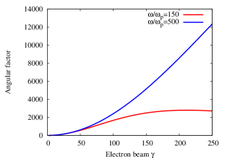
Figure 1: Dependence of the angular factor with the electron beam’s relativistic factor $\gamma$ for two values of $\omega/\omega_{p}$ with $\omega_{p}=38$eV. The lower value $\omega/\omega_{p}$ corresponds to an X-ray energy of 5.7 keV and the higher value to a X-ray energy of 19keV.

The atomic structure function $F(g)$ and consequently the susceptibility are calculated from the expressions

$$F(g) = f_{0}(s)+(f^{{}^{\prime}}+if^{{}^{\prime\prime}}),\;\;\;f_{0}(s)=\sum_{i}a_{i}\exp[-b_{i}s^{2}]+c,\;\;\;\;\;s=4\pi g$$

$$\chi_{0} = -\frac{\lambda^{2}r_{e}N_{C}}{\pi V_{C}}[f^{{}^{\prime}}+if^{{}^{\prime\prime}}],\;\;\;\;\chi_{g}=-\frac{\lambda^{2}r_{e}}{\pi V_{C}}[(f_{0}(s)+f^{{}^{\prime}}-Z)+if^{{}^{\prime\prime}}]S_{hkl}$$ (9)

The coefficients $(a_{i},b_{i},c)$ are the Cromer-Mann coefficients [15] while the frequency dependent form factors $(f^{{}^{\prime}},f^{{}^{\prime\prime}})$ can be obtained from a database maintained by NIST [16]. Here $r_{e}$ is the classical electron radius, $N_{C}$ is the number of atoms in the unit cell, $V_{C}$ is the volume of the unit cell, $Z$ is the atomic number of the crystal and $S_{hkl}$ is the crystal structure factor for the plane with indices $(h,k,l)$. The photon attenuation length at a wavelength $\lambda$ can be found from $L_{a}=\lambda/(2\pi|{\rm Im}(\chi_{0})|)$.

We now discuss the geometric factor $f_{geo}$ in Eq.(4). The unit vectors $\hat{n},\hat{v},\hat{\Omega}$ are defined and shown in Fig.2.

Figure 2: Left: A general crystal geometry for an arbitrary orientation of the reflecting plane. Reciprocal lattice vector ${\bf g}$: normal to the crystal plane, n: normal to the crystal surface. Bragg geometry corresponds to the crystal plane which has ${\bf g}||{\bf n}$, Laue geometry to ${\bf g}\perp{\bf n}$. Right: The different angles between ${\bf g}$, ${\bf n}$, ${\bf v}$: electron velocity vector, and ${\Omega}$: direction of the detector’s central axis

The figure on the left in Figure 2 shows the electron velocity vector v, the normal ${\bf n}$ to the crystal surface, and the normal ${\bf g}$ to the crystal planes. The figure on the right in Figure 2 shows the direction of the detector’s central axis $\bm{\Omega}$, and the angles between the vectors. It is clear that in order for the crystal plane to be a reflecting plane, the angle $\pi/2-\theta_{B}$ between ${\bf g}$ and -v and also the angle $\phi$ between ${\bf g}$ and $\bm{\Omega}$ must satisfy $0\leq(\pi/2-\theta_{B},\phi,\zeta)\leq\pi/2$ where $\zeta$ is the angle between ${\bf g}$and n. Bragg geometry corresponds to $\zeta=0$ while in Laue geometry $\zeta=\pi/2$. If $\theta_{D}$ is the angle of the detector relative to the velocity vector v, then we have

$$\phi=\frac{\pi}{2}-(\theta_{D}-\theta_{B}),\;\;\;\hat{n}\cdot\hat{v}=-\sin(\theta_{B}+\zeta),\;\;\;\;\hat{n}\cdot\hat{\Omega}=\sin(\theta_{D}-\theta_{B}-\zeta)$$

The geometric factor $f_{geo}$ in the intensity expression can then be written as

$$f_{geo}=L_{a}|\frac{\sin(\theta_{D}-\theta_{B}-\zeta)}{\sin(\theta_{B}+\zeta)}|[1-\exp(-\frac{t}{L_{a}|\sin(\theta_{D}-\theta_{B}-\zeta)|})]$$ (10)

Note that if $\theta_{D}=\theta_{B}+\zeta$, the geometric factor $f_{geo}=0$ because the photons travel along the larger transverse dimensions of the crystal and will be mostly absorbed in the crystal.

We mention here that a refinement to the kinematical theory is the dynamical diffraction theory [17, 18, 19] which takes into account the coupling between the photon fields with wave vectors ${\bf k_{i}}$ and ${\bf k_{f}+g}$ via interaction with the crystal. This coupling gives rise to additional PXR photons emitted in the forward direction in close proximity to the electron beam. This forward PXR was observed in experiments at the Mainz laboratory [20] but care was required to extract this PXR emission signal as transition radiation and bremsstrahlung are also emitted in the same direction. We will not discuss this forward PXR emission here as it does not offer the relatively background free property of PXR emission at the Bragg angle.

3 Energy spectrum broadening

The intensity spectrum given by Eq.(7) predicts a delta function spectrum at integer multiples $m\omega_{B}$ of the Bragg frequency. In practice, there are several mechanisms which broaden the frequency of each line in the spectral distribution. We discuss the important sources and present analytical results for their contributions to the energy width and compare them to previous experimental results.

3.1 Geometric effects

Figure 3: Effect of the beam spot size (a) and crystal thickness (b) on the angular photon spread. In (a), the beam spot diameter is represented by $s_{0}$ and $s_{D}$ is its projection on the detector. In (b), the crystal thickness is $t$, the effective thickness traversed by the electrons is $t_{eff}$ and $t_{D}$ the projection on the detector.

From Eq.(3), it follows that the photon energy depends on the angle of the incident electron and the photon direction. The incident angle will have a finite spread due to the beam divergence while the photon angle hitting the detector can have a spread due to several effects including the finite beam spot size on the crystal surface, the detector size and the crystal thickness.

Writing the spread in electron incident angle in the diffraction plane as $\Delta\alpha_{x}$ and the photon angle as $\theta_{D}=2\theta_{B}+\theta_{x}$, we have from Eq.(3) to first order in $\Delta\alpha_{x}$

$$(\frac{\Delta E}{E})_{div}=\frac{1}{2\sin^{2}\theta_{B}}\theta_{x}\Delta\alpha_{x}$$ (11)

We set $\Delta\alpha_{x}=\sigma_{x}^{{}^{\prime}}$ the beam divergence in the diffraction plane and $\theta_{x}=\Delta x_{det}/R$ where $\Delta x_{det}$ is the width of the detector and $R$ is the distance from the crystal to the detector.

Again from Eq.(3), it follows that the energy spread is related to the photon angular spread as

$$(\frac{\Delta E}{E})_{D}=\frac{\Delta\theta_{D}}{\tan\theta_{B}}$$ (12)

The impact of the finite beam size on $\Delta\theta_{D}$ can be seen in Fig.3a. A finite size on the crystal surface projects to a spot size on the reflecting planes from which photons with a spread of angles can reach the detector. Let $s_{0}$ be the beam spot diameter on the crystal and $s_{p}$ its projection on the crystal’s reflecting plane. The angle the velocity vector $\hat{v}$ makes with the crystal surface is $\theta_{B}+\zeta$, hence it follows from the figure that

$$s_{1}=s_{0}\sin(\theta_{B}+\zeta),\;\;\;s_{p}=\frac{s_{1}}{\cos(\pi/2-\theta_{B})},\;\;\;\Rightarrow s_{p}=\frac{\sin(\theta_{B}+\zeta)}{\sin{\theta_{B}}}s_{0}$$

On reflection from the crystal plane, the size $s_{p}$ projects to a size $s_{D}=s_{p}\sin(\theta_{D}-\theta_{B})$. The angular spread in the photon angles resulting from the beam size is

$$(\Delta\theta_{D})_{size}=\frac{s_{D}}{R}=\frac{\sigma_{x}}{R}\frac{\sin{\theta_{B}+\zeta}}{\sin\theta_{B}}\sin(\theta_{D}-\theta_{B})$$ (13)

where we have replaced $s_{0}$ by the rms beam size $\sigma_{x}$.

The impact of the finite crystal thickness is seen in Fig.3b. The effective crystal thickness $t_{eff}$ projects to a length on the detector $t_{D}=t_{eff}\sin\theta_{D}=t\sin\theta_{D}/\sin(\theta_{B}+\zeta)$ where $t$ is the crystal thickness. Hence the angular spread in photon angles due to the crystal thickness is

$$(\Delta\theta_{D})_{crystal}=\frac{t_{D}}{R}=\frac{t}{R}\frac{\sin\theta_{D}}{\sin(\theta_{B}+\zeta)}$$ (14)

Finally the detector size results in an angular spread $(\Delta\theta_{D})_{det}=\Delta x_{det}/R$.

Adding the independent sources of beam angle spread and photon angle spread in quadrature, the energy spread due to these geometric effects is

$$\frac{\Delta E}{E}=\frac{1}{R}\left[(\frac{\Delta x_{det}\sigma_{x}^{{}^{\prime}}}{2\sin^{2}\theta_{B}})^{2}+\cot^{2}\theta_{B}\left\{(\sigma_{x}\sin(\theta_{B}+\zeta))^{2}+(t\frac{\sin 2\theta_{B}}{\sin(\theta_{B}+\zeta)})^{2}+(\Delta x_{det})^{2}\right\}\right]^{1/2}$$ (15)

Here we have set $\theta_{D}=2\theta_{B}$, the direction for specular reflection. For typical beam and crystal parameters, the dominant contributions are from the beam spot size and the detector width while the contributions from the beam divergence and crystal thickness are significantly smaller.

3.2 Multiple Scattering

The contribution of multiple Coulomb scattering can be analytically calculated from the differential angular spectrum. Using Eq.(4), it follows that the differential angular spectrum per unit length is given by

$$\frac{d^{3}N}{dz\;d\theta_{x}\;d\theta_{y}}=\frac{\alpha_{f}}{4\pi c}\frac{\omega_{B}}{\sin^{2}\theta_{B}}\frac{1}{|\hat{n}\cdot\hat{v}|}\exp[-\frac{z}{L_{a}|\hat{n}\cdot\hat{\Omega}}]e^{-M(g)}|\chi_{g}(\omega)|^{2}\frac{\theta_{x}^{2}\cos^{2}2\theta_{B}+\theta_{y}^{2}}{[\theta_{x}^{2}+\theta_{y}^{2}+\theta_{ph}^{2}]^{2}}$$ (16)

The spread in angles $\theta_{x},\theta_{y}$ changes as the electron beam propagates through the crystal due to multiple scattering. Assuming the multiple scattering process to be Gaussian, the angles are sampled from distributions

$$f(\theta_{x})=\frac{1}{\sqrt{2\pi}\sigma_{x}^{{}^{\prime}}}\exp[-\frac{\theta_{x}^{2}}{2\sigma_{x}^{{}^{\prime}2}}]$$

and a similar expression for the distribution in $\theta_{y}$. Here $\sigma_{x}^{{}^{\prime}},\sigma_{y}^{{}^{\prime}}$ are the rms beam divergences which increase with $z$ as the beam propagates through the crystal. Writing the initial beam divergences as $(\sigma_{x,0}^{{}^{\prime}},\sigma_{y,0}^{{}^{\prime}})$, the $z$ dependent divergences are

$$\sigma_{x}^{{}^{\prime}}(z)=[(\sigma_{x,0}^{{}^{\prime}})^{2}+(\sigma_{MS}^{{}^{\prime}}(z))^{2}]^{1/2}$$

and similarly for $\sigma_{y}^{{}^{\prime}}$. Here $\sigma_{x,MS}$ is the rms multiple scattering angle in the $x$ direction. This can be found from the expression [21]

$$\sigma_{MS}^{{}^{\prime}}(z)=\frac{13.6}{E_{e}}\sqrt{\frac{z}{X_{rad}}}[1+0.038\log(\frac{z}{X_{rad}})]$$ (17)

where $z$ is the path length traversed in the crystal,$E_{e}$ is the electron beam energy in MeV and $X_{rad}$ is the radiation length.

The multiple scattering weighted distribution function in $\theta_{x}$ is then

$$(\frac{dN}{d\theta_{x}})_{MS} = \int dz\int d\phi_{x}\int d\theta_{y}f(\phi_{x})\frac{d^{3}N}{dzd\theta_{x}d\theta_{y}}(z,\phi_{x},\theta_{x}\theta_{y})$$ (18)

$$= {\cal A}\int dz\int d\phi_{x}\int d\theta_{y}\frac{1}{E(\theta_{x}+\phi_{x})}\frac{1}{\hat{n}\cdot\hat{v}}\exp[-\frac{z}{L_{a}|\hat{n}\cdot\hat{\Omega}}]$$

$$\frac{1}{\sigma_{x}^{{}^{\prime}}(z)}\exp[-\frac{\phi_{x}^{2}}{2\sigma_{x}^{{}^{\prime}2}}]\frac{\theta_{x}^{2}\cos^{2}2\theta_{B}+\theta_{y}^{2}}{[\theta_{x}^{2}+\theta_{y}^{2}+\theta_{ph}^{2}]^{2}}$$

Here ${\cal A}$ includes all factors which do not depend on $z,\theta_{x},\theta_{y}$. Within the integrand, $E(\theta_{x}+\phi_{x})$ denotes that the photon energy is evaluated at the angle $(\theta_{x}+\phi_{x})$. From this weighted distribution, the average and rms width of the energy spectrum can be found as

$$\langle E\rangle = \frac{\int EdN}{\int dN}=\frac{\int E(dN/d\theta_{x})_{MS}d\theta_{x}}{\int(dN/d\theta_{x})_{MS}d\theta_{x}}$$

$$\sigma_{E,MS}^{2} = \langle E^{2}\rangle-\langle E\rangle^{2}$$ (19)

We will use Eq.(19) to estimate the energy width due to multiple scattering instead of a Monte-Carlo simulation that is often used.

There is another contribution to the linewidth from the photo-absorption in the crystal. Assuming a point source electron beam and no imperfections or multiple scattering, the photon wave train emitted by the beam has an intrinsic energy width given by [22]

$$\Delta E_{Intrinsic}=\hbar\omega\frac{\chi_{0,I}}{2\sin^{2}\theta_{B}}=\frac{\hbar c}{2\sin^{2}\theta_{B}L_{a}}$$ (20)

where $\chi_{0,I}$ is the imaginary part of the mean dielectric susceptibility. The intrinsic width has a minimum value for backward emission when $\theta_{B}=\pi/2$. This contribution is typically orders of magnitude smaller than the other contributions discussed above.

The expressions for the energy width have been checked against measured values from a couple of earlier experiments, one at a low beam energy of 6.8MeV [23] and the other with beam energy of 56 MeV [24], close to the FAST beam energy of 50 MeV. Since multiple scattering is more important at lower energy, comparison with the low energy result are a good check of the width from multiple scattering while the second case will be a good check of the geometrical width. Table 1 shows the results of the comparison.

Crystal	Geometrical	Multiple Scattering	Intrinsic	Theory(total)	Experiment
	[eV]	[eV]	[eV]	[eV]	[eV]
C (111)	35.9	34.8	2.1$\times 10^{-4}$	49.4	51
Si (220)	524.9	61.3	2.8$\times 10^{-4}$	529	540 $\pm$ 120
Si (400)	97.1	9.7	2.1$\times 10^{-3}$	98	134 $\pm$ 56

Table 1: Comparison of theoretical energy widths with experimental values after removing the effects of the detector energy resolution. First row: Experiments with 6.8 MeV electrons and a diamond crystal [23]. Second and third rows: Experiments with 50-60 MeV electrons and silicon crystals [24, 25]. These values are taken from Table 36 in [24]. The theoretical estimates include geometrical, multiple scattering and intrinsic contributions added in quadrature.

The geometrical linewidth was calculated using Eq.(15) and the multiple scattering contribution using Eqs.(18) and (19). The two were then added in quadrature to yield the theoretical value shown in Table 1.

4 Angular spectrum broadening

The measured angular intensity distribution represents a convolution of the intrinsic PXR intensity with the Gaussian response of the detector angular resolution, the beam divergence and multiple scattering. Hence the measured intensity is of the form

$$\frac{d^{2}N}{d\theta_{x}\theta_{y}}_{conv}(\theta_{x},\theta_{y})=\frac{A_{C}}{2\pi\sigma_{x}^{T}\sigma_{y}^{T}}\int\frac{d^{2}N}{d\theta_{x}\theta_{y}}(\theta_{x}-q_{x},\theta_{y}-q_{y})\exp[-(\frac{q_{x}}{\sqrt{2}\sigma_{x}^{T}})^{2}-(\frac{q_{y}}{\sqrt{2}\sigma_{y}^{T}})^{2}]dq_{x}dq_{y}$$ (21)

where $A_{C}$ is a constant to ensure photon number conservation after the convolution, $d^{2}N/d\theta_{x}\theta_{y}$ is the angular distribution without convolution, and the total angular resolutions $\sigma_{x}^{T},\sigma_{y}^{T}$ are given by

$$\sigma_{u}^{T}=\sqrt{(\frac{\sigma_{D,u}}{R})^{2}+(\sigma_{u}^{{}^{\prime}})^{2}+(\sigma_{MS}^{\prime})^{2}}$$ (22)

where $u=(x,y)$, $\sigma_{D,u}$ is the detector resolution, $R$ is the distance of the detector from the crystal, $\sigma_{u}^{{}^{\prime}}$ is the beam divergence at the crystal, $\sigma_{MS}^{{}^{\prime}}$ is the effective multiple scattering angle averaged over the path length $t/\cos\theta_{B}$.

In the absence of the broadening due to the convolution, the intrinsic angular width of he PXR spectral distribution is given by $\Delta\theta_{PXR}\simeq\theta_{ph}$. In crystals with thicknesses comparable to the attenuation length, the broadening due to multiple scattering is significant and the characteristic double peaked angular distribution is replaced by a broadened single peak distribution with the center filled in.

Other sources of angular broadening are the higher order reflections from planes with spacings which are integer sub-multiples of the primary plane. These higher order reflections produce higher photon energies with lower yield leads to a broadened distribution when recorded on a detector which sums over all photon energies.

5 Spectral Brilliance

The spectral brilliance of the photon beam is defined as the number of photons emitted per second per unit area of the photon beam per unit solid angle per unit relative bandwidth

$$B=\frac{d^{4}N}{dtdAd\Omega d\omega/\omega}$$ (23)

Expressed in conventional light source units, the average spectral brilliance can be written in terms of the averaged beam parameters and differential angular intensity spectrum per electron in a 0.1% bandwidth

$$B_{av} = \frac{d^{2}N}{\hbar d\omega d\Omega}\frac{I_{av}}{e}\frac{E_{\gamma}}{(\sigma_{\gamma})^{2}}*10^{-3}$$ (24)

$$= \frac{I_{av}}{e}\frac{1}{\Delta E_{\gamma}/E_{\gamma}}\frac{dN}{d\Omega}\langle\frac{1}{\sigma_{e}^{2}}\rangle\times 10^{-15}\;\;\;{\rm photons/s-(mm-mrad)^{2}-0.1\%BW}$$ (25)

where $I_{av}$ is the average electron beam current, $E_{\gamma}$ is the energy of the X-ray line and $\sigma_{\gamma}$ is the X-ray beam spot size. In the second line $dN/d\Omega$ is the angular yield in units of photons/(el-sr), and we set the photon spot size to the electron beam spot size in the crystal, i.e. $\sigma_{\gamma}=\sigma_{e}$. Here $\Delta E_{\gamma}$ includes only the contributions to the spectral width from the crystal but not that from the detector resolution.

Due to multiple scattering within the crystal, the electron beam divergence, beam size and emittance will grow as the electrons move through the crystal. Writing $\epsilon_{N}$ as the normalized electron emittance, the emittance growth as a function of the distance traversed $z$ is

$$\Delta\epsilon_{N,x}(z)=\gamma\beta_{x}(\sigma_{MS}^{{}^{\prime}}(z))^{2}$$ (26)

where $\beta_{x}$ is the optical beta function at the crystal in the $x$ axis, If the initial beam size at the crystal is $\sigma_{x,0}$ and the normalized emittance at the crystal entrance is $\epsilon_{N,0}$, then $\beta_{x}=\gamma(\sigma_{x,0}^{2}/\epsilon_{N,0}$. The beam divergence grows as $\sigma_{e}^{{}^{\prime}}(z)=\sqrt{(\sigma_{e}^{{}^{\prime}}(0))^{2}+(\sigma_{MS}^{{}^{\prime}}(z))^{2}}$ and the average of the inverse beam size squared follows from

$$\langle\frac{1}{\sigma_{e}^{2}}\rangle\equiv\frac{\gamma}{\beta_{x}}\langle\frac{1}{\epsilon_{N}(z)}\rangle=\frac{\gamma}{\beta_{x}t_{eff}}\int_{0}^{t_{eff}}dz\;\frac{1}{[\epsilon_{N,0}+\gamma\beta_{x}(\sigma_{MS}^{{}^{\prime}}(z))^{2}]}$$ (27)

This averaged expression will be used in Eq.(25) for the average brilliance. If the initial beam divergence and beam emittance are small compared to their increase through the crystal, and neglecting the logarithmic correction to the multiple scattering angle , we have $(\sigma_{e}(z),\sigma_{e}^{{}^{\prime}}(z)\propto\sqrt{z}$ and the emittance grows as $\epsilon_{N}(z)\propto z$.

Since the brilliance scales linearly with the electron current but inversely as the square of the electron spot size, it is advantageous to geneate as small a spot size as feasible even at the cost of reducing the beam current. Since the emittance grows with crystal thickness faster than the yield does, the maximum brilliance will also require the use of thin crystals, as will be shown later with numerical examples.

6 PXR in FAST

Parameter	Value	Units
Beam energy	50	MeV
Bunch charge	20	pC
Length of a macropulse	1	ms
Number of bunches/macropulse	2000	-
Macropulse repetition rate	5	Hz
Bunch frequency	2	MHz
Interval between bunches	0.33	$\mu$s
Bunch length	3	ps
Crystal, thickness	Diamond, 168	$\mu$m

Table 2: Bunch and macropulse parameters in FAST

In the FAST beamline, a goniometer on loan from the HZDR facility, described in [26], is presently available. It has two ports through which radiation can be extracted - one along the beam axis which will be used for channeling radiation and another at 90^∘ to the beam axis which can be used to extract PXR. This determines that with the detector angle at 90 degrees, the Bragg angle must be 45 degrees in order to generate PXR with sufficient intensity.

The goniometer already has a diamond crystal inside with its surface cut parallel to the (1,1,0) plane to generate channeling radiation from this plane. It has a thickness of 168$\mu$m and this will be the assumed value for most calculations reported here. In order to limit heating the crystal by the beam, we will assume low current operation with an average beam current of 200nA and a bunch charge of 20pC. At such charge values, low transverse emittance of the order of 100 nm can be obtained by suitably shaping the laser spot on the cathode [27] or alternatively with field emission cathodes [11]. The main parameters of FAST and the crystal are shown in Table 2. We choose $R=1$ m as the crystal to detector distance and the active size of the detector plate to be 2cm x 2cm.

Table 3 shows the PXR photon energies, the angular yield and the energy width from reflection off three of the possible low order planes with a 50 MeV electron beam. The yields include the effect of attenuation in air from the crystal to the detector. The reciprocal lattice spacing $g$ between adjacent planes with indices $(h,k,l)$ is found from $g=(2\pi/a)\sqrt{h^{2}+k^{2}+l^{2}}$ where $a$ is the length of a unit cell. Consequently both the energy and absolute linewidths increase with increasing order. The yields are higher for the (2,2,0) and the (4,0,0) planes primarily due to the higher susceptibility $\chi_{\bf g}$.

Plane	X-ray energy	$L_{a,C}$	$L_{a,air}$	Attenuation	Yield	$\Delta E$
	[keV]	[cm]	[cm]	in air	[photons/el-sr]	[eV]
(1,1,1)	4.26	0.0097	12.72	3.8$\times 10^{-4}$	3.7$\times 10^{-7}$	59
(2,2,0)	6.95	0.043	57.2	0.17	9.9$\times 10^{-5}$	93
(4,0,0)	9.83	0.120	144.9	0.50	8.8$\times 10^{-5}$	131

Table 3: Photon yields and linewidths at a Bragg angle of 45^∘, observation angle of 90^∘ in FAST from PXR off some planes. Bragg geometry in all cases, crystal thickness = 0.168mm. The relative energy width in all cases is about 1%. The yield value includes the effect of attenuation over a 1m long path in air from the crystal to the detector.

Table 4 shows linewidth contributions from geometric effects and multiple scattering for each of the planes. The two effects are comparable in these cases.

Plane	Geometrical Width (eV)	Multiple-Scattering(eV)	Total (eV)
(111)	42.8	39.3	59.1
(220)	69.5	62.0	93.2
(400)	98.3	86.7	131.1

Table 4: Contributions to the energy width from geometric effects and multiple scattering.

Figure 4 shows the two dimensional contour plots of the angular intensity spectrum projected on the $(\theta_{x},\theta_{y})$ axes without and with convolution. The broadening effects are clearly visible as the two distinct peaks in the left figure merge into a single wider maxima in the right figure.

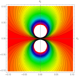
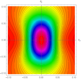
Figure 4: Contour plots of the differential yields as functions of $(\theta_{x},\theta_{y})$ without broadening (left) and with broadening(right). The white areas in the left figure correspond to the highest intensities. The convolution lowers the peak intensities and results in a central broad peak instead of the two peaks without convolution. Both figures are for the (2, 2, 0) plane with a Bragg angle of 45^∘ and a beam divergence of 1mrad. These contour plots correspond to the images that would be observed on a detector plate.

For each primary plane, PXR emission also occurs from higher order planes at higher energies and lower intensities. For the (1,1,1) plane, the next allowed higher order plane is the (3,3,3) plane, since $S(g)=0$ for the (2,2,2) plane. The photon energy from the (3,3,3) plane is 12.8 keV with significantly reduced attenuation in air and resulting in a angular yield at the detector about two orders of magnitude higher than that from the (1,1,1) plane. For the (220) plane, second order reflections from (440) are allowed with photon energy of 13.9keV. The (440) plane has an angular yield about a third smaller than the (220) plane even after including smaller attenuation at the higher energy. For the (400) plane, the second order reflection from the (800) plane produces 19.7keV photons and an angular yield about 10% that of the first order yield. The broadening of the angular distributions from the higher order reflections in these cases is found to be insignificant.

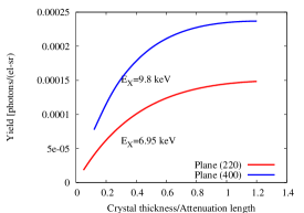
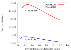
Figure 5: Left: Yield per electron per steradian as a function of the crystal thickness relative to the photon attenuation length in the crystal for two different planes: (220) and (400). Photon attenuation lengths in the crystal are: 431 $\mu$m at 6.9keV, and 1198$\mu$m at 9.8keV. Right: Spectral brilliance as a function of the relative crystal thickness for the two planes.

Figure 5 shows the impact of the crystal thickness on the angular yield and spectral brilliance for two different planes. The thickness is shown relative to the photon attenuation length, this length is larger for the (400) plane because of the higher photon energy. For the same absolute thickness, the angular yield with the (220) plane is larger, as seen in Table 3 for a single thickness but the angular yield for the same relative crystal thickness is higher with the (400) plane because the absolute thickness is larger. In both cases, the angular yield appears to saturate at a thickness of about 1.2$L_{a}$. The spectral brilliance for the same relative crystal thickness is larger with the (2,2,0) plane because the average emittance over the crystal is smaller with a smaller absolute thickness. In both cases, the brilliance reaches a maximum around (0.2 - 0.3)$L_{a}$. These plots show that the optimum crystal thickness depends on whether the photon yield or the spectral brilliance is the object of interest.

6.1 New Goniometer

The initial set of experiments will be conducted with the goniometer described above with the two ports. There is another goniometer under construction which will have a total of five ports through which X-rays could be extracted. A schematic of this new goniometer is shown in Figure 6.

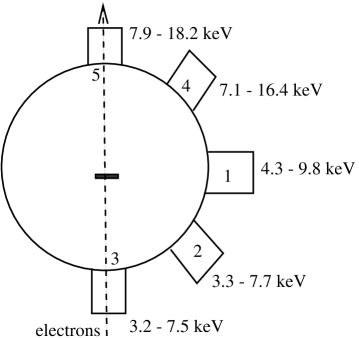
Figure 6: Schematic of the new goniometer with the five labeled ports. The X-ray energies expected from these ports with different planes, see Table 5, are also shown. Note: Ports 3 and 5 are not in the horizontal plane but are 45^∘ to the horizontal. There is an exit port under port 5 and in the horizontal plane but not shown here.

These ports will offer the opportunity of generating PXR at different Bragg angles and hence different energies, yields and spectral brilliance from those considered in the previous subsection.

The angle of the port determines the direction of the photon emission and hence the vector $\vec{\Omega}$. We write the unit vector along the detector axis as $\hat{\Omega}=(\omega_{1},\omega_{2},\omega_{3})/\sqrt{\omega_{1}^{2}+\omega_{2}^{2}+\omega_{3}^{2}}$. If the PXR plane has Miller indices $(h,k,l)$, the unit normal $\hat{g}$ can be one of $\pm(h,k,l)/\sqrt{h^{2}+k^{2}+l^{2}}$. The conditions for reflection require that both $\hat{g}\cdot(-\hat{v})\geq 0$ and $\hat{g}\cdot\hat{\Omega}\geq 0$. The first of these results in choosing the sign of $\hat{g}$ while the second determines if a chosen detector angle is suitable for observing reflected photons. Together the two conditions ensure that the incident beam and the reflected photons are on the same side of the reflecting plane. For a given plane with a normal $\hat{g}$, the Bragg angle is determined from $\theta_{B}=\arcsin[-\hat{v}\cdot\hat{g}]$. For the goniometer ports shown in Figure 6, the angle vectors to the detector locations are

$$\hat{\Omega}_{1} = (1,0,0),\;\;\;\hat{\Omega}_{2}=(\sin(13\pi/18),0,\cos(13\pi/18)),\;\;\;\hat{\Omega}_{3}=(0,\frac{1}{\sqrt{2}},-\frac{1}{\sqrt{2}}),$$

$$\hat{\Omega}_{4} = (\sin(5\pi/18),0,\cos(5\pi/18)),\;\;\;\hat{\Omega}_{5}=(0,\frac{1}{\sqrt{2}},-\frac{1}{\sqrt{2}})$$

Energies and angular yields at the different ports from different PXR planes are shown in Table 5.

Port	Plane 111		Plane 220
	Energy	Ang. Yield	Energy	Ang. Yield
	[keV]	[$\times 10^{-5}$ phot/e--sr ]	[keV]	[$\times 10^{-5}$ phot/e--sr ]
1	4.3	0.037	6.9	9.9
2	3.3	3.4$\times 10^{-5}$	5.4	1.2
3	3.2	1.5$\times 10^{-5}$	5.3	0.096
4	7.1	76.9	11.6	90.5
5	7.9	142	12.8	108.3
Port	Plane 311		Plane 400
	Energy [keV]	Ang. Yield	Energy [keV]	Ang. Yield
	[keV]	[$\times 10^{-5}$ phot/e--sr ]	[keV]	[$\times 10^{-5}$ phot/e--sr ]
1	8.1	5.3	9.8	8.8
2	6.4	1.6	7.7	4.8
3	6.2	1.4	7.5	4.6
4	13.6	26.5	16.4	34.7
5	15.1	41.3	18.2	40.8

Table 5: X-ray energies at the different ports for different PXR reflection planes. Bragg geometry is assumed in all cases.

Port	Plane 111			Plane 220
	Energy	$t/L_{a}$	Sp. Br. [$\times 10^{8}$]	Energy	$t/L_{a}$	Sp. Br. [$\times 10^{8}$]
4	7.1	0.36	5.5	11.6	0.09	2.2
5	7.9	0.26	5.7	12.8	0.07	2.1
Port	Plane 311			Plane 400
	Energy	$t/L_{a}$	Sp. Br. [$\times 10^{8}$]	Energy	$t/L_{a}$	Sp. Br. [$\times 10^{8}$]
4	13.6	0.06	0.59	16.4	0.04	0.59
5	15.1	0.05	0.57	18.2	0.03	0.56

Table 6: PXR photon energy, crystal thickness $t$ relative to attenuation length $L_{a}$, and spectral brilliance (Sp. Br.) in units of photons/s-(mm-mrad)²- 0.1% BW] at ports 4 and 5 for different planes. The crystal thickness was 0.168mm in each case.

Table 6 shows the spectral brilliance expected from ports 4 and 5, the ones corresponding to the smallest Bragg angles and highest yields. With the crystal thickness kept constant at 0.168 mm, the spectral brilliance is highest for the (111) plane at these ports. The X-ray energy is between 7-8 keV and the ratio of the crystal thickness to attenuation length is close to the optimal value of around 0.2, seen in Figure 5. For the higher order planes, the PXR energy increases but the spectral brilliance decreases. Especially for planes (3,1,1) and (4,0,0) the brilliance drops by an order of magnitude compared to the (1,1,1) plane. This is partly due to the small relative thickness and increasing the crystal thickness would also increase the brilliance, but not significantly. The choice of plane would then be determined by whether higher energy or higher brilliance is more desirable. A higher energy beam, e.g. 100MeV, would increase the yield and also the brilliance because the emittance growth due to multiple scattering would also be smaller.

6.2 PXR while channeling

It was pointed out [28] that if a beam is channeled within a crystal and emits channeling radiation, it may also emit PXR emission from reflection off complementary planes which intersect the channeling planes. It has subsequently been observed at the SAGA light source linac with 255 MeV electron beams [29]. Here we consider the prospect of detecting PXR emission under channeling conditions while using the present goniometer. As mentioned previously, this goniometer has a second port at 90^∘ to the beam axis which could be used for detection of PXR. These requirements impose constraints on the possible PXR planes and the orientation of the crystal which we now consider.

Figure 7: Sketch of the (110) channeling plane, the $(1,\bar{1},1)$ plane which is one of the possible PXR planes, the electron beam direction and the direction of the PXR photons from this reflection plane.

Choosing the $(110)$ plane as the channeling plane, the unit normal to this plane is $\hat{m}=(1,1,0)/\sqrt{2}$. This vector must be normal to the velocity vector which could be of the form $\hat{v}=(a,-a,c)/\sqrt{2a^{2}+c^{2}}$ where $(a,c)$ are arbitrary real numbers. We will consider two choices below, one with $(a,c)=(-1,0)$ and another with $(a,c)=(0,1)$. If the PXR plane is $(1\bar{1}1)$, the unit normal to the PXR plane is $\hat{g}=(1,-1,1)/\sqrt{3}$ and the Bragg angle $\theta_{B}$ is determined by the condition $\sin\theta_{B}=|\hat{g}\cdot\hat{v}|=|(2a+c)/(\sqrt{3(2a^{2}+c^{2})})|$. The choice $\hat{v}=(-1,1,0)/\sqrt{2}$ yields $\theta_{B}={\rm arcsin}(\sqrt{2/3})=54.7^{\circ}$ while choosing the vector $\hat{v}=(0,0,1)$ yields $\theta_{B}={\rm arcsin}(\sqrt{1/3})=35.3^{\circ}$. A smaller Bragg angle leads to a higher PXR photon energy, so we choose $\hat{v}=(0,0,1)$. In practice, with a given electron beam direction, these choices will correspond to different orientations of the crystal with respect to the beam velocity. For particles at other angles in the beam distribution, the requirement for channeling is that the velocity vector has an angle smaller than the critical angle $\theta_{C}$, i.e. $\theta={\rm arcsin}(\hat{m}\cdot\hat{v})<\theta_{C}$.

If we assume that the crystal has been cut so that the surface is parallel to the channeling plane, then the unit normal to the surface, defined as $\hat{n}$ (see Fig. 2) is identical to the vector $\hat{m}$ defined above, i.e. $\hat{n}=\hat{m}=(1,1,0)/\sqrt{2}$.

6.2.1 Crystal rotation

If the crystal is aligned with so that the channeling plane is parallel to the velocity vector, then the Bragg angle with a chosen PXR plane may not be appropriate to observe the PXR photons at 90 degrees to the beam. However, a rotation of the crystal about an axis orthogonal to the channeling plane can create the desired Bragg angle while maintaining the channeling condition. If the rotation matrix about the normal to the channeling plane $\hat{m}$ is written as $R(\psi)$ where $\psi$ is the rotation angle, then the rotated normal to the PXR plane is $\hat{g}_{R}=R(\psi)\hat{g}$. The requirement on this angle $\psi$ is that the velocity has the desired Bragg angle with the new normal $g_{R}$, i.e.

$$\sin\theta_{B}=\hat{g}_{R}\cdot(-\hat{v})\equiv R(\psi)\hat{g}\cdot(-\hat{v})$$ (28)

The rotation matrix about an arbitrarily chosen unit vector $\hat{\mu}=(\mu_{x},\mu_{y},\mu_{z})$ is the so-called Rodrigues matrix [30] given by

$$R(\psi)=\left[\begin{array}[]{ccc}\cos\psi+\mu_{x}^{2}S&-\mu_{z}\sin\psi+\mu_{x}\mu_{y}S&\mu_{y}\sin\psi+\mu_{x}\mu_{z}S\\ \mu_{z}\sin\psi+\mu_{x}\mu_{y}S&\cos\psi+\mu_{y}^{2}S&-\mu_{x}\sin\psi+\mu_{y}\mu_{z}S\\ -\mu_{y}\sin\psi+\mu_{x}\mu_{z}S&\mu_{x}\sin\psi+\mu_{y}\mu_{z}S&\cos\psi+\mu_{z}^{2}S\end{array}\right]$$ (29)

where $S=2\sin^{2}(\psi/2)$. When the channeling plane is (110), the rotation axis is $\hat{\mu}=(1,1,0)/\sqrt{2}$. The desired angle of rotation $\psi$ is found from Eq.(28) with $\theta_{B}=\pi/4$.

Applying this to different possible PXR planes will ensure that the rotated light vector lies in the $(x,y)$ plane. A further rotation about the $z$ axis (i.e along the beam direction) may be necessary to direct the light out along the $x$ axis. When the emitted light as viewed at an angle 2$\theta_{B}$ to the beam, the reflected light vector prior to any rotations is $\hat{\Omega}=\hat{v}-2(\hat{g}.\hat{v})\hat{g}$ while that after rotation is $\hat{\Omega}_{R}=\hat{v}-2(\hat{g}_{R}\cdot\hat{v})\hat{g}_{R}$.

As an example, consider the plane $(\bar{1},1,1)$ for PXR production. Choosing the normal to this plane as $\hat{g}=(1,-1,-1)/\sqrt{3}$, we have

$$\hat{g}_{R}\cdot(-\hat{v})=\frac{1}{\sqrt{3}}(\cos\psi+\sqrt{2}\sin\psi)=\frac{1}{\sqrt{2}}\Rightarrow\psi=9.74^{\circ},\hat{\Omega}_{R}=\frac{1}{\sqrt{2}}(1,-1,0)$$

In this case, a rotation by $\psi=9.74^{\circ}$ about the normal to the channeling plane and a further rotation by $\phi=45^{\circ}$ about the beam axis will direct the PXR light out of the port along the positive $x$ axis.

Table 7 shows some of the low order planes, the angles of rotation $\psi$ and $\phi$, and the energies of the emitted X-rays into the detector. This table shows that the $(2,0,\bar{2})$ plane would be the simplest as it does not require any rotation of the crystal while it is oriented for channeling. Another reason for choosing this plane is that with rotation, the path length of the beam while channeling will be different compared to the unrotated case and could affect the channeling yield.

Plane	Angle$\psi$[deg]	Angle $\phi$[deg]	$E_{X}$[keV]
$(\bar{1},1,1)$	9.74	45	4.26
$(1,\bar{1},1)$	-9.74	135	4.26
(2, 0. 2)	0	180	6.95
$(2,0,\bar{2})$	0	0	6.95
$(0,2,\bar{2})$	0	-90	6.95
(0,0,4)	45	135	9.83

Table 7: PXR planes, the angles of rotation $\psi$ about the normal to the channeling plane (1,1,0) and $\phi$, angle of rotation about the beam direction so that the PXR light is directed out of the port along the positive $x$ direction at 90 degrees to the beam axis. The energy of the PXR light is also shown. Other low-order planes not shown are those for which no rotation will direct the X-ray beam in the desired direction.

The angle $\zeta$ between the unit normal $\hat{n}$ to the surface and the unit normal $\hat{g}$ to the channeling plane will change depending on the channeling plane chosen. We assume here as above that the crystal is cut parallel to the channeling plane so that $\hat{n}=(1,1,0)/\sqrt{2}$. The angle between the two is given by $\zeta=\arccos(\hat{n}\cdot\hat{g})$, thus for the $(2,0,\bar{2})$ PXR plane, this angle is 60^∘.

6.2.2 Yield and spectral brilliance

The above analysis has shown that with the crystal oriented for channeling along the (1,1,0) plane, PXR emission from the (2,0,$\bar{2}$) plane can be obtained at 90^∘ to the beam direction without any crystal rotation. In the subsequent discussion, we will primarily consider PXR from this plane.

When beam energies are under 100 MeV, the channeling radiation spectrum consists of a few well defined lines and is best understood as arising from transitions between bound states of the transverse potential. We consider planar channeling and the $x$ direction to be orthogonal to the channeling plane. The quantum mechanical states are then found from solutions of the one dimensional Schrodinger equation,

$$[-\frac{\hbar^{2}}{2m_{e}\gamma}\frac{\partial^{2}}{\partial x^{2}}+V(x)]\psi(x)=E_{\perp}\psi(x)$$ (30)

Here $V(x)$ is the one dimensional continuum potential obtained by averaging the three dimensional atomic potential along the orthogonal directions $(y,z)$.

Parametric X-rays emitted under channeling conditions (PXRC) are considered to be those in which the electrons stay within the same transverse energy band, i.e with only intra-band transitions. PXR emitted while electrons transition between different energy bands is labeled as diffracted channeling radiation (DCR) and has apparently not yet been experimentally observed. We will only consider the yield from PXRC here.

The angular spectrum of PXRC is related to that of PXR by [31]

$$\frac{d^{2}N}{d\theta_{x}\theta_{y}}|_{PXRC}=\frac{d^{2}N}{d\theta_{x}\theta_{y}}|_{PXR}\sum_{n}^{N_{B}}P_{n}|F_{nn}|^{2}$$ (31)

where the sum over the states $n$ ranges over the total number of bound states $N_{B}$. Here we also include the effects of a finite beam divergence, so we define $P_{n}$ the initial probability of occupation of state $n$ by averaging over the beam divergence. It is given by

$$\langle P_{n}\rangle=\frac{1}{\sqrt{2\pi}\sigma_{x}^{{}^{\prime}}}\frac{1}{d_{p}}\langle\int d\phi_{x,0}\exp[-\frac{\phi_{x,0}^{2}}{2(\sigma_{x}^{{}^{\prime}})^{2}}]|\int_{-d_{p}/2}^{d_{p}/2}\exp[-ik\phi_{x,0}x]\psi_{n,K_{C}}(x)dx|^{2}\rangle_{K_{C}}$$ (32)

Here $\sigma_{x}^{{}^{\prime}}$ is the beam divergence in the channeling plane, $d_{p}$ is the inter-planar separation, $k$ is the initial momentum wavenumber of the incident particle, $\phi_{x,0}$ is the angle of incidence with respect to the channeling plane and $\psi_{n,K_{C}}$ is the wave function in the $n$th state with transverse wavenumber $K_{C}$ where $-g/2\leq K_{C}\leq g_{2}$. Since this wave function also depends upon the band wavenumber $K_{C}$ in the Brillouin zone, the average $\langle\rangle_{K_{C}}$ on the right hand side represents an average over the wavenumbers in the Brillouin zone.

The form factor $F_{nn}$ describes the impact of the channeling wave functions on the PXR yield and is defined as [28]

$$F_{nn}=\langle\psi_{n}|\exp[-ik_{x}x]|\psi_{n}\rangle$$

where $k_{x}$ is the transverse component of the photon wave vector. We can therefore define the averaged form factor squared as

$$\langle|F_{nn}(\theta_{x})|^{2}\rangle=\frac{1}{d_{p}^{2}}\langle|\int_{-d_{p}/2}^{d_{p}/2}\psi_{n,K_{C}}^{*}(x)\exp[-i\frac{\omega_{B}\theta_{x}x}{c}]\psi_{n,K_{C}}(x)dx|^{2}\rangle_{K_{C}}$$ (33)

Here $\theta_{x}$ is the angle of photon emission in the horizontal plane with respect to the direction of specular reflection and we average over the Brillouin zone as before.

The quantum mechanical calculations were done with a Mathematica notebook used at the ELBE facility to study channeling [32] and significantly corrected and modified for use at FAST, as described in [3]. The transverse function is expanded in a Fourier series using the lattice periodicity as

$$V(x)=\sum_{n=-\infty}^{\infty}V_{n}\exp[ingx]$$ (34)

The Fourier coefficients $V_{n}$ are obtained from the Doyle-Turner coefficients $(a^{DT},b^{DT})$ [33] as

$$V_{n}=-\frac{2\pi}{V_{c}}a_{0}^{2}(\frac{e^{2}}{a_{0}})e^{-M(\vec{g})}\sum_{j}e^{i\vec{g}\cdot\vec{r}_{j}}\sum_{i=1}^{6}a_{i}^{DT}\exp[-\frac{b_{i}^{DT}}{16\pi^{2}}(ng)^{2}]$$ (35)

Here $V_{c}$ is the volume of the unit cell, $a_{0}$ is the Bohr radius, $\vec{r}_{j}$ are the coordinates of the $j$th atom in the unit cell and $M(\vec{g})=\frac{1}{2}g^{2}\langle u^{2}\rangle$ is the Debye-Waller factor (mentioned earlier with Eq.(7) in Section 2) describing thermal vibrations with mean squared amplitude $\langle u^{2}\rangle$, assumed to be the same for all atoms. The wave functions are found by first expanding them in a series of Bloch functions and then solving the resulting matrix eigenvalue problem, see e.g [34].

The wave functions are then subsequently used in calculating the correction factors defined above. The form factor $\langle|F_{nn}(0)|^{2}\rangle=1$ and we find that in the range $-3/\gamma\leq\theta_{x}\leq 3/\gamma$, $\langle|F_{nn}(\theta_{x})|^{2}\rangle\approx 1$ to within 0.2% in all cases. The significant correction for the PXRC yield is due to the initial probability of occupation $\langle P_{n}\rangle$ which is determined by the beam divergence. This population of the bound states decreases as the beam divergence approaches the critical angle of channeling which at the FAST energy of 50MeV is about 0.98mrad. The correction $\delta$ is defined as the relative difference between the PXR and PXRC yields, hence as $\delta=1-\sum_{n}^{N_{B}}\langle P_{n}\rangle\langle|F_{nn}|^{2}\rangle$. This correction factor increases with beam divergence and has the values 0.02, 0.09 and 0.58 at beam divergences of 0.01mrad, 0.1mrad and 1mrad respectively.

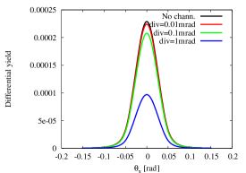
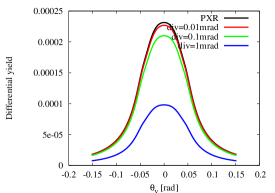
Figure 8: The differential yield as a function of the photon emission angle $\theta_{x}$ (left) and $\theta_{y}$ (right) without channeling and with channeling for three values of the initial beam divergence. The channeling plane was (1,1,0) and the PXR plane was (2,0,$\bar{2}$). Convolution broadening was included in all cases.

Plane	Divergence	$\Delta E$	Yield		Spectral Brilliance
	mrad	eV	$\times 10^{-4}$ photons/(e--sr)		photons/(mm-mrad)2-0.1% BW
			PXR	PXRC	PXR	PXRC
(2,0,$\bar{2}$)	0.01	93	0.40	0.38	35.9	35.1
	0.1	93	0.40	0.35	2.1$\times 10^{5}$	1.9$\times 10^{5}$
	1.0	93	0.40	0.16	6.5$\times 10^{8}$	1.8$\times 10^{8}$
(0,0,4)	0.01	131	0.89	0.85	21.3	20.8
	0.1	131	0.89	0.78	1.27 $\times 10^{5}$	1.14 $\times 10^{5}$
	1.0	131		0.37	4.25 $\times 10^{8}$	1.2$\times 10^{8}$

Table 8: Comparison of angular yields, photon flux and spectral brilliance without and with channeling for three values of the initial beam divergence and for two PXR planes. The channeling plane was fixed at (1,1,0). Angle $\zeta=60^{\circ}$ for the (2,0,$\bar{2}$) plane, and $\zeta=90^{\circ}$ (Laue geometry) for the (0,0,4) plane. The energy width is affected by the PXR plane but not by the initial beam divergence.

Figure 8 shows the angular spectra from PXRC for the three divergences mentioned and compared with the spectrum from PXR without channeling. Table 8 shows that the angular yield decreases with beam divergence, because the fraction of particles in the bound states decreases with increasing divergence. Since the spectral brilliance is inversely proportional to the square of the spot size and assuming the emittance is conserved, a larger beam divergence implies a smaller spot size. The increase in brilliance with the smaller spot size dominates the decrease due to channeling.

6.3 Possible applications of PXR

One of the primary foreseen uses of PXR is in phase contrast imaging (PCI) of low Z materials, specially biological samples. There are many PCI methods, we plan to use the free space propagation method which does not need any additional optical elements. The principle of PCI is that phase shifts undergone by hard X-rays when traversing low Z samples are orders of magnitude larger than absorption effects. The phase shift changes the complex amplitude of the wave field and hence causes intensity modulations when undergoing interference with X-rays that have not passed through the sample. The quality of the image with the free space propagation method depends on the source size, the geometric magnification and the resolution of the detector. Th special feature of FAST that makes it suitable for PCI is the very low emittance of the electron beam, and hence the small X-ray source size after the crystal. With electron emittances around 100nm using a conventional photocathode, beam sizes at the crystal around 1-5 $\mu$m can be achieved [35]. This compares very favorably with recent PCI experiments using PXR [36] which had beam sizes of 0.5 - 2 mm (FWHM) at the target. With the use of field emitter nanotips as the cathode, the beam emittance could be improved another order of magnitude [11] implying a further improvement in image resolution. The use of the new goniometer, discussed in Section 6.1 will enable imaging at multiple X-ray energies.

Finally, we mention a proposal [37] to generate short electron bunches at FAST using a slit mask placed in the middle of the bunch compressor chicane. Sub-picosecond electron bunches could be produced without the need of an undulator or an additional complex laser system. Due to scattering in the mask, the final beam intensity will only be about 10% of the initial intensity. However, starting from initial intensities of 1-3 nC, the final bunch intensities within the bunch train will be low enough (about 20 pC) for PXR generation. The resulting sub-picosecond X-ray pulses will have a higher peak brilliance and could be used for time resolved X-ray studies in materials science, chemistry and biology.

7 Conclusions

In this paper we considered the prospect of generating PXR using diamond crystals with 50 MeV electron beams from the photoinjector at the FAST facility at Fermilab. We revisited calculations of the energy width from both geometric and multiple scattering. Comparisons with earlier experiments were found to yield reasonable agreement The PXR spectrum model calculation was applied to the conditions at FAST. Using the presently available goniometer restricts the Bragg angle to 45^∘ but allows a clear separation from the electron beam. The PXR energies from the planes studied fall in the range 4 - 10 keV with a spectral energy widths of $\sim 1$%. With a diamond crystal thickness of 168$\mu$m, maximum angular yields are about 10^-4 photons/e^--sr, taking into account attenuation in air from the crystal to the detector. Using crystals of different thicknesses, the PXR yield was found to saturate at a thickness of about 1.2$L_{a}$, the photon attenuation length at two different energies. The spectral brilliance on the other hand attained a maximum value at around 0.2$L_{a}$ for these same energies. This is mainly because the emittance growth over larger thicknesses reduces the brilliance more than the yield increases it. Next, PXR emission with a new goniometer with five possible ports was studied. The range of energies now spans 3 - 18 keV. The spectral brilliance, around 10⁸ photons/(mm-mrad)²-0.1% BW, is reached with a fixed crystal thickness which is less than 0.2$L_{a}$ for most energies, so higher brilliance is feasible with thicker crystals. Use of this goniometer would open up the possibility of extracting PXR at multiple energies simultaneously. Finally, PXRC or PXR under channeling conditions was studied and the yield with quantum corrections from channeling was calculated for three beam divergences. While the reduction in PXR yield during channeling was smallest for the lowest divergence, higher brilliance favors the smallest beam spot size or equivalently the largest divergence under conditions of equal emittances. This PXRC emission makes possible simultaneous X-ray emission from channeling and PXR at 90 degrees to each other. The brilliance of PXR appears to be sufficient for phase contrast imaging and the FAST facility with (10 - 100) nm scale electron emittances should enable imaging with very good resolution.

Acknowledgments
We thank the Lee Teng undergraduate internship program at Fermilab which awarded T. Seiss a summer internship in 2014. Fermilab is operated by Fermi Research Alliance under DOE Contract No. DE-AC02-07-CH11359.

References

- [1] E. Harms et al, ICFA Beam Dynamics Newslett. 64, 133 (2014);
- [2] D. Mihalcea et al, Proc. IPAC15 (2015)
- [3] T. Sen and C. Lynn, Int. J. Mod. Phys. A, 29, 1450179 (2014)
- [4] M.L. Ter-Mikaelian, High energy electromagnetic processes in condensed media, Wiley Interscience, New York (1972)
- [5] V.G. Baryshevsky and I.D. Feranchuk, Sov. Phys. JETP, 34, 502 (1972)
- [6] A.N. Didenko et al, Phys. Lett. A, 110, 177 (1985)
- [7] P. Rullhusen et al, Novel Radiation Sources using Relativistic Electrons, World Scientific Publishing Co. (1998)
- [8] V.G. Baryshevsky et al, Parametric X-Ray Radiation in Crystals, Springer (2005)
- [9] W. Scandale et al, Phys. Lett. B, 701, 180 (2011)
- [10] W. Gabella et al, Nucl. Instrum, & Meth. B309, 10 (2013)
- [11] P. Piot et al, Appl. Phys. Lett., 104, 263504 (2014)
- [12] I.D. Feranchuk and I.V. Ivashin, J. Phys (Paris), 46, 1981 (1985)
- [13] H. Nitta, Phys. Lett. A, 158, 270 (1991)
- [14] K. Brenzinger et al, Z. Phys. A,358, 107 (1997)
- [15] D.T. Cromer and J.B. Mann. Act Crys. A24, 321 (1968)
- [16] C.T. Chantler, X-ray form factor, attenuation and scattering tables,J. Phys.Chem.Ref.Data 24,71 (1995); Table at http: physics.nist.gov/PhysRefData/FFast/html/form.html
- [17] V.G. Baryshevsky and I.D. Feranchuk, Sov. Phys. JETP 34, 502 (1972)
- [18] G.M. Garibian and C. Yang, Sov. Phys. JETP, 34, 495 (1972)
- [19] A. Caticha, Phys. Rev. A, 40, 4322 (1989)
- [20] H. Backe et al, Nucl. Instr. & Meth. B, 234, 138 (2005)
- [21] J. Beringer et al (Particle Data Group), Phys. Rev. D,86, 010001 (2012)
- [22] A. Caticha, Phys. Rev. B, 45, 9541 (1992)
- [23] J. Freudenberger et al, Appl. Phys. Lett. 70,267 (1997)
- [24] B Sones PhD thesis, Rensselaer Polytechnic Inst., Troy, NY (2004)
- [25] B. Sones et al, Nucl. Instr & Meth A, 560, 589 (2006)
- [26] W. Wagner et al, Nucl. Instr. & Meth. B266, 327 (2008)
- [27] R.K. Li et al, Phys. Rev. ST-AB, 15, 090702 (2012)
- [28] R. Yabuki et al, Phys. Rev. B, 63, 174112 (2001)
- [29] Y. Takabayashi et al, Nucl. Instr. & Meth. B, 315, 105 (2013)
- [30] O. Rodrigues, J. Math. Pures. Appl. 5, 380 (1840)
- [31] K.B. Korotchenko et al, JETP, 95, 481 (2012)
- [32] B. Azadegan, Comp. Phys. Comm., 184, 1064 (2013)
- [33] R.A. Doyle and P.S. Turner, Acta Crystallogr. A , 24, 390 (1968)
- [34] B. Azadegan et al, Phys. Rev B.,74, 045209 (2006)
- [35] P. Piot et al, AIP Conf. Proc. 1507, 732 (2012)
- [36] Y. Hayakawa et al, J. Inst. 8, C08001 (2013)
- [37] J.C. Thangaraj and P. Piot, arxiv:1310.5389