A MODEL OF LANGUAGE INFLECTION GRAPHS

Abstract

Inflection graphs are highly complex networks representing relationships between inflectional forms of words in human languages. For so-called synthetic languages, such as Latin or Polish, they have particularly interesting structure due to abundance of inflectional forms. We construct the simplest form of inflection graphs, namely a bipartite graph in which one group of vertices corresponds to dictionary headwords and the other group to inflected forms encountered in a given text. We then study projection of this graph on the set of headwords. The projection decomposes into a large number of connected components, to be called word groups. Distribution of sizes of word group exhibits some remarkable properties, resembling cluster distribution in a lattice percolation near the critical point. We propose a simple model which produces graphs of this type, reproducing the desired component distribution and other topological features.

PACS Nos.: 64.60.ah, 05.90.+m, 05.70.Jk, 02.50.-r, 64.60.aq

1 Introduction

Human languages can be studied from many different perspectives. If we think of a foreign language, however, we typically think of words of that language, thus it is quite natural that vocabulary is one of the most extensively studied features of languages. In recent years, the network paradigm has been used to study vocabularies, and within this paradigm, words of the language are viewed as vertices of a large and complex network or graph, with edges representing relationships between words. Many such models emphasizing different relationships between words have been studied in the past decade, including networks of co-occurrences of words in sentences[1], thesaurus graphs[2, 3, 4], WordNet database graphs[5], and many others[6, 7, 8, 9, 10].

It is fair to say that a lot of the aforementioned works concentrated on the English language, which has a very characteristic property of being analytic, that is, exhibiting only a minimal inflection. In analytic languages grammatical relations and categories are handled mostly by the word order, and not by the inflection, thus making them somewhat easier to learn.

In contrast to this, synthetic languages such as Latin, Greek, Polish, or Russian make an extensive use of inflection, and one word in these languages can appear in great many forms, reflecting grammatical categories such as tense, mood, person, number, gender, case, etc. Order of words is less important in synthetic languages. While this is an excellent feature from the point of view of a poet, it presents algorithmic problems in text processing. Let us suppose, for example, that we want to count the number of distinct words in a given work – e.g., for the purpose of comparing two works and deciding which one uses larger vocabulary. How do we do this in a language like Latin, where one dictionary headword can have as many as hundred different forms? To make things even more difficult, in some cases, one inflectional form can correspond to more than one dictionary headword, and one must deduce from the context which one to choose.

In Ref. paper38, one of the authors considered this problem from a practical point of view, and proposed a solution which exploits some features of the so-called inflection graph. Here we will not dwell on this problem, referring an interested reader to Ref. paper38, but we will instead discuss the inflection graph itself. We will first describe some of its topological features, and then propose a model which reproduces these features.

2 Inflection graphs

The inflection graph for a given language can be constructed as follows. First we need to create a list of all words of the language, which, strictly speaking, is an impossible task, as every such list is bound to be incomplete. Nevertheless, one can easily obtain a reasonably adequate list of words using sufficiently large dictionary of the language. The set of all dictionary headwords will be denoted by $H$. For each headword, we generate a list of all possible inflected forms, and the list of all possible inflected forms obtained this way will be denoted by $I$. We then construct a bipartite graph $G=(H,I,E)$, where $E$ is the set of edges such that the edge between $v\in H$ and $u\in I$ exists if and only if $u$ is an inflected form of $v$.

Construction of the inflection graph is obviously possible only if one is able to produce all inflected forms of a given word. For the Latin language, this can be achieved using WORDS, a computerized dictionary of Latin created by William Whitaker[12]. The resulting bipartite graph has $1\,028\,972$ vertices and $1\,077\,806$ edges, and will be denoted by $G_{LA}$.

We were also able to construct inflection graph for Polish language, using lexical grammar developed by the Group of Computer Linguistics of AGH University of Science and Technology in Kraków[13]. The corresponding graph, to be denoted by $G_{PL}$, has $1\,872\,140$ vertices and $802\,911$ edges.

Normally, for most headwords in $H$, there are many corresponding inflected forms in $I$, so an element of $H$ is typically connected to many (sometimes 100 or more) elements of $I$. For example, the Latin word dicunt (they say) and dixit (he said) are both inflected forms of the verb dico, thus we will have a vertex in $H$ corresponding to dico connected to vertices in $I$ corresponding to dicunt and dixit. However, the opposite can also be true: in some instances, a word can be an inflected form of more than one headword, so that vertices of $I$ are sometimes connected to more than one vertex of $H$. As an example, consider the word sublatus, which could be a form of tollo (lift, raise) or suffero (bear, endure), thus a vertex in $I$ corresponding to sublatus will be connected to two vertices in $H$.

The inflection graphs are rather sparse, and they decompose into a large number of connected components of different sizes. From the practical point of view, the size of the component is not as important as the number of distinct headwords in the component, which we will call headword groups. The motivation for this can be explained as follows.

Suppose that one wants to perform a computerized count of the number of different words occurring in a given text. Obviously, one wants to count two different inflection forms of a given word as one and the same word, or, to put this differently, one wants to know how many distinct dictionary headwords appear in the text (in various inflected forms). However, since in languages with a complex inflection system a given inflection form can sometimes belong to two (or more) different dictionary headwords, it is impossible for a computer to decide which one is used in a particular case. To make such a decision, one has to understand the sentence and figure out from the context what is means. In English this problem is quite rare, but still exists. For example, consider the word dove – this could be the singular form of the noun dove (a type of bird), or the simple past tense of the verb to dive. Computer program upon encountering dove in a text will not know whether to count it as occurence of the headword dove or to dive. The simple solution to this problem is to say that dove is an inflected form of a headword from the set (headword group) {dove, to dive}. This means that instead of counting how many distinct headwords are present in the text, we can only count how many distinct headword groups are present. We want to know, however, what are the sizes of the headword groups, as it is, in a sense, a measure of the difficulty of the disambiguation problem. A good way to analyze these sizes is to look at their distribution.

The distribution of headword groups sizes in inflection graphs is quite striking, as can be seen in Figure 1, which shows the distributions for Latin and Polish. The graph for Latin and its analysis have been previously published in Ref. paper38, here we add the same graph for Polish language.

We fitted a straight line in log-log coordinates to data points for which the number of groups exceeds 20, in order to exclude points with small count. The lines of the best fit are shown as dashed lines. There seems to be a power-law trend in both data, more strongly pronounced in the graph for the Latin language. In the remaining part of this paper we will attempt to shed some light on the origin of this phenomenon.

The dashed lines of the best fit shown in Figure 1 represent the power law

$$n_{s}\sim s^{-\tau},$$ (1)

where $\tau\approx-3.1\pm 0.3$ for Latin and $\tau\approx-4.3\pm 0.9$ for Polish. Errors given for $\tau$ signify that decreasing/increasing $\tau$ by the given amount increases the reduced $\chi^{2}$ twice.

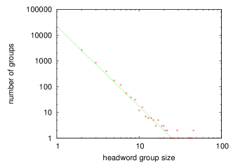
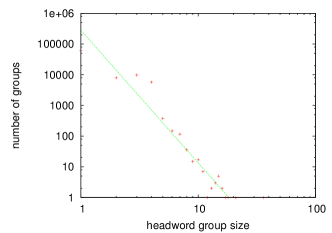
Figure 1: Distribution of headword clusters for Latin (left) and Polish (right). Slope of the fitted line is, correspondingly, $-3.1\pm 0.3$ and $-4.3\pm 0.9$. The figure for Latin previously appeared in Ref. paper38

Anyone who is familiar with the percolation theory[14, 15] can immediately recall that a very similar scaling law for cluster sizes holds for the lattice percolation at the critical point, where $\tau$ is known as the Fisher exponent[14]. This is also the case for the Erdös-Rényi model $G(n,p)$, that is, a graph constructed by connecting $n$ nodes randomly so that each edge is included in the graph with probability $p$ independent from every other edge.

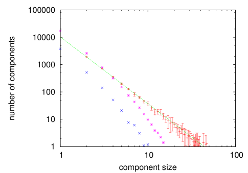
Figure 2: Distribution of component sizes for the random graph averaged over 10 realizations of the graph above ($\times$), below ($\star$), and at the percolation threshold ($+$). The data point corresponding to the giant component above the percolation threshold is not shown. Slope of the fitted line is $-2.44\pm 0.09$. Error bars correspond to standard deviations, and for clarity are shown only for the data at the critical point.

It is well known that at $np=1$ and $n\to\infty$ the model undergoes a structural transition similar to percolation[16]. The distribution of component sizes follows the power law of eq. (1), and the Fisher exponent is known[17] to be $\tau=2.5$. Figure 2 shows component size distributions obtained numerically for $G(n,p)$ with $n=28092$, that is, the same $n$ as the number of headwords in $G_{LA}$. Three values of $np$ were used, $np=0.5$ (below the percolation threshold), $np=2.0$ (above the percolation threshold) and $np=1.0$ (at the percolation threshold). The power law in the form of eq. (1) is evident at the percolation threshold, yet it is clearly not valid away from the threshold. In spite of the fact that the number of vertices is relatively small and that only 10 graphs were generated, the value of the exponent $\tau=2.44\pm 0.09$ obtained from fitting the straight line to data agrees, within error bounds, with the aforementioned value of $\tau=2.5$.

Considering the case of $G(n,p)$, one could suspect that the inflection graphs have a structure somewhat resembling Erdös-Rényi random graphs at the percolation threshold. We will, however, demonstrate that this is somewhat more complicated. To avoid repetitions, from now on we will be using $G_{LA}$ as an example.

3 Structure of the inflection graph for Latin

In order to describe some important features of $G_{LA}$, we will consider its projection on $H$. Given a bipartite graph $G=(H,I,E)$, define its $H$-projection as $G^{\prime}=(H,E^{\prime})$, where $\{u,v\}$ is in $E^{\prime}$ if and only if $u$ and $v$ are both connected to a common vertex in $I$. $H$-projection of $G_{LA}$ has 28092 vertices and 24064 edges. Only 13345 headwords have degree greater than zero in $G_{LA}^{\prime}$. Note that for obvious reasons, distribution of component sizes of $G_{LA}^{\prime}$ is the same as the distribution of group sizes in $G_{LA}$. Could it then be that $G_{LA}^{\prime}$ resembles Erdös-Rényi random graph?

In order to answer this question, we will first consider the degree distribution of $G_{LA}^{\prime}$ shown in Figure 3. Unlike in the case of $G(n,p)$, the degree distribution of $G_{LA}^{\prime}$ is clearly not Poissonian, and for small degree values it seems to follow exponential decay, shown in the figure as a straight line. The mean vertex degree is $1.8$. This already indicates that $G(n,p)$ cannot be a model of $G_{LA}^{\prime}$ – the mean vertex degree of $G(n,p)$ with a power law distribution of components sizes must be equal to 1.0.

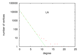
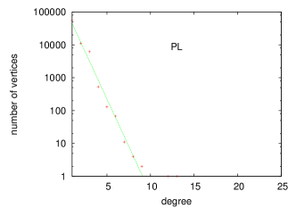
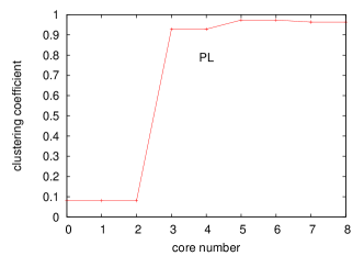
Figure 3: Degree distribution (left) and clustering coefficients of cores (right) of $H$-projection of $G_{LA}$ (top) and $G_{PL}$ (bottom).

We can see the difference between $G(n,p)$ and $G_{LA}^{\prime}$ even better if we use the notion of core clustering spectrum, introduced in Ref. paper37. For a non-negative integer $k$, the $k$-core of a graph is the maximal subgraph such that its vertices have degree greater or equal to $k$. By the “degree” in this definition we mean the degree of the vertex in the subgraph. If $G$ is a given graph, we denote by $G_{\{k\}}$ the $k$-core of $G$. Now let $C(G)$ denote the clustering coefficient of $G$. A set of pairs $(|G_{\{k\}}|,C(G_{\{k\}}))$, where $|G|$ denotes the number of vertices of $G$, will be called core clustering spectrum of $G$. One can visualize the core clustering spectrum by plotting points $(|G_{\{k\}}|,C(G_{\{k\}}))$ on a plane, as it has been done in Ref. paper37. Here we will use slightly different graphs in order to convey a similar information, namely we will plot $C(G_{\{k\}})$ as a function of $k$. We will call it the graph of clustering coefficients of cores. This has the advantage over the plot of core spectrum in having the core number explicitly as one of the variables. The value of $k$ will range from $1$ to $k_{max}$, where $k_{max}$ is the largest $k$ for which $G_{\{k\}}$ is non-empty.

For some graphs, such as the Erdös-Rényi random graphs, most vertices belong to the same $k$-core, as documented in Ref. Alvarez2005. This means that the graph of clustering coefficients of cores for Erdös-Rényi random graphs is very narrow, consisting of only a small number of points. This is not the case for $G_{LA}^{\prime}$, as Figure 3 attests. $G_{LA}^{\prime}$ possesses highly clustered inner core, feature absent in Erdös-Rényi model near the percolation threshold.

Degree distribution of $G_{PL}^{\prime}$ and its graph of clustering coefficients of cores are quite similar to corresponding graphs of $G_{LA}^{\prime}$, as shown in the bottom of Figure 3.

4 Model

In order to construct a model of inflection graphs which exhibits power law scaling resembling Figure 1, as well as having the degree distribution and clustering coefficients of cores of its $H$-projection resembling Figure 3, we need to make a couple of further remarks regarding topological structure of inflection graphs, again using $G_{LA}$ as an example. It is useful to think of $G_{LA}$ as a collection of stars, each centered at a headword and with arms connecting the headword to some inflected forms. These stars are not completely disjoint, however. Sometimes they share one or more vertices in $I$, and this occurs if a given headword shares some of its inflected forms with another headword (or headwords).

Let $n$ be the number of headwords, and $m$ be the number of inflected forms. Construction of the random graph serving as a model of $G_{LA}$ proceeds in two stages. In stage 1, we generate an assembly of stars, each centered at a headword and with arms connecting the headword to some inflected forms. In stage 2, we generate a number of random bridges between these stars. We now describe the two stages in detail.

Algorithm for generating stars

1. Generate the set of vertices $H=\{H_{1},H_{2},\ldots,H_{n}\}$ corresponding to headwords, and another set $I=\{I_{1},I_{2},\ldots,I_{m}\}$ corresponding to inflected forms.

2. For each $i\in\{1,2,\ldots n\}$, draw a random number $x_{i}$ from a distribution $f_{h}$ to be described below, and connect vertex $H_{i}$ to vertices $I_{j+1},I_{j+2},\ldots,$ $I_{j+\lfloor|x_{i}|\rfloor}$, where $j=0$ for $i=1$ and $j=\sum_{p=1}^{i-1}{\lfloor|x_{p}|\rfloor}$ otherwise. If any vertex index in $I_{j+1},I_{j+2},\ldots,$ $I_{j+\lfloor|x_{i}|\rfloor}$ exceeds $m$, it is replaced by its value modulo $m$.

3. If any isolated vertices in $I$ still remain, connect each of them to a randomly selected vertex in $H$. After this is done, relabel the set $I$ so that vertices connected to the same headword are labeled with a block of consecutive integers.

The probability distribution function $f_{h}$ is a weighted sum of three normal distributions,

$$f_{h}(x)=\sum_{i=1}^{3}w_{i}f_{\sigma_{i},\mu_{i}}(x),$$ (2)

where

$$f_{\sigma,\mu}(x)=\frac{1}{\sigma\sqrt{2\pi}}e^{\frac{-(x-\mu)^{2}}{2\sigma^{2}}}.$$ (3)

We used values $(w_{1},w_{2},w_{3})=(0.68,0.28,0.04)$, $(\mu_{1},\mu_{2},\mu_{3})=(8,90,3)$ and $(\sigma_{1},\sigma_{2},\sigma_{3})=(2,10,1)$. These were obtained by fitting the resulting degree distribution to the degree distribution of the actual inflection graph, but their values are not too critical, meaning that small changes in values of these parameters still produce graphs with power-law distribution of headword group sizes.

Note that although the random number $x_{i}$ drawn from the distribution $f_{h}$ in step two may theoretically be zero, yet the probability of such event is extremely small. In our program implementing the algorithm for generating stars, we simply reject $x_{i}=0$ outcome and draw another number if it happens.

The reason for taking $f_{h}$ to be the sum of three normal distributions is the structure of Latin vocabulary. With respect to inflection, one can distinguish three main groups of words: (1) verbs (inflexion by conjugation), (2) nouns and adjectives (inflection by declension) and (3) all other words. We should remark here that this shape of the distribution is suitable for Latin, but for a different language, with a different grammatical structure, it would have to be different – in particular, the number of normal distributions in the sum would likely have to change. Moreover, we used normal distribution for the sake of simplicity, and we do not claim that this reflects the actual distribution of inflection forms very accurately, but it is close enough for our purposes. One should also note that $f_{h}$ may theoretically produce negative numbers (again, with very small probability), and this is why we take the absolute value of $x_{i}$. We also round $x_{i}$ down to the nearest integer. One could use in place of the normal distribution some other distribution with strongly pronounced peak and producing only positive numbers, such as, for example, the log-normal distribution. We found, however, that the detailed shape of the distribution is not too crucial for our goal of reproducing the desired properties of the inflection graph, thus we kept the normal distribution for simplicity.

Once the assembly of stars is created, we add a number of bridges between the stars. The most crucial feature of these bridges comes from the fact that typically two headwords share not one, but many inflected forms with another headword or headwords. This is because there exists a large number of pairs of closely related Latin words, each having a separate entry in the dictionary. For example, the words dico (say), dictum (utterance, remark) and dictus (speech) are all closely related, thus they share many inflected forms. After experimenting with many possible methods for generation of bridges, we came out with a simple algorithm, which basically adds a fixed number of edges at a time.

Let $\lambda$ and $T$ be two positive integers, to be used as parameters in our algorithm.

Algorithm for generating bridges

1. Randomly select two headword vertices $H_{a}$ and $H_{b}$, where by $H_{a}$ we denoted the vertex with the larger degree. Vertex $H_{a}$ is already connected to $k$ inflected forms, let us denote them by $\{I_{r},I_{r+1},\ldots I_{r+k-1}\}.$

2. Add $\lambda$ additional edges by connecting $H_{b}$ with vertices $\{I_{r},I_{r+1},\ldots I_{r+\lambda-1}\}$.

3. Repeat the above two steps $T$ times.

Note that the second step is performed exactly as described even if $\lambda>k$, but in this case some of the inflected forms with which we connect $H_{b}$ will not be inflected forms of $H_{a}$, but inflected forms of some other word(s). Also note that $k$ is always greater than zero, because the algorithm for generating stars ensures that this is the case. This agrees with our interpretation of the meaning of the “inflected form”. We assume that every word has at least one inflected form – if it is an adverb, for example, its sole “inflected form” is identical to itself. This is consistent wit the treatment of other parts of the speech. For instance, for nouns we count nominative singular among inflected forms, even though it is identical to the headword form.

Regarding the value of $\lambda$ and $T$, they must be selected as follows. After completing the algorithm for generating stars, the number of edges in the graph is only slightly larger than $|I|$ (recall that in step 2 we are replacing indices exceeding $m$ with their values modulo $m$, but this happens only rarely for a few values of $i$ close to $n$). Of course it could theoretically happen that the number of vertices will be larger than the desired number of edges (we want to have the same number of edges in the model graph as in the inflection graph being modeled). With the choice of parameters which we have made, the probability of such event is so exceedingly small, that for all practical purposes we can simply ignore such eventuality. Nevertheless, if it indeed happened, one would have to discard the result and run the algorithm for generating stars again.

Having less than the desired number of edges, we must ensure that the product $\lambda T$ is equal to the number of remaining edges which we want to produce. This means that only one of those two parameters can be freely chosen. By experimenting with different values of $\lambda$ in the range from $1$ to $15$, we found that $\lambda=10$ produces the most clearly pronounced power-law distribution of headword sizes in the resulting graph. The typical corresponding value of $T$ in this case is $T=7692$. We say “typical” because, as explained earlier, the exact number of vertices in the graph obtained after applying the algorithm for generating stars will slightly fluctuate for different realizations of the graph, thus the number of “missing vertices”, and consequently the value of $T$, will slightly fluctuate too. The shape of the headword group size distribution graph, however, is only weakly affected by changes of $\lambda$ and $T$ as long as their product remains equal to the number of “missing vertices” and providing that $\lambda>1$. For example, if instead of $\lambda=10$ and $T=7692$ we use $\lambda=5$ and $T=15384$, there is almost no perceptible difference in the shape of the graph.

We generated random graph following the above algorithm using $|H|=28092$ and $|I|=1000880$, that is, the same number of vertices as in the actual inflection graph. This graph will be called $G_{MOD}$. Its distribution of headword group sizes is shown in Figure 4. Agreement with the actual distribution shown in Figure 1 is indeed very good. Even the slope of the fitted line agrees (within the error bound) with the exponent observed in $G_{LA}$, as these are respectively $-3.4\pm 0.5$ and $-3.1\pm 0.3$.

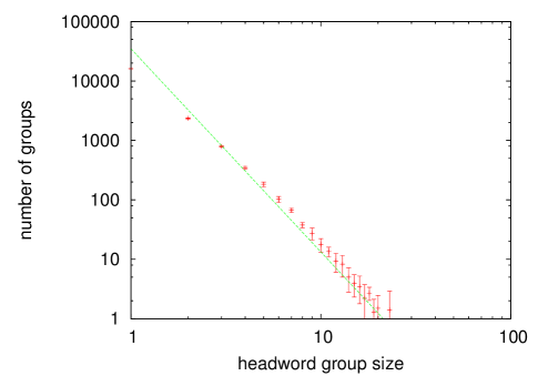
Figure 4: Distribution of headword group sizes for the model graph $G_{MOD}$ averaged over 10 realizations of the graph. Slope of the fitted line is $-3.4\pm 0.5$.

The model also performs well when one considers $H$-projection of $G_{MOD}$. Figure 5 shows both the degree distribution and the graph of clustering coefficients of cores of $G_{MOD}^{\prime}$. Comparing these graphs with Figure 3, we can observe good qualitative agreement.

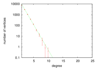
Figure 5: Degree distribution (left) and clustering coefficients of cores (right) of $H$-projection of the model graph, averaged over 10 realizations of the graph. Error bars correspond to standard deviation.

Degree distribution of $G_{MOD}^{\prime}$ is very similar to degree distribution of $G_{LA}^{\prime}$, except that $G_{MOD}^{\prime}$ misses a small number of high-degree vertices, present in $G_{LA}^{\prime}$. Clustering coefficients of cores of both graphs exhibit very similar behavior, that is, the clustering sharply increases with increasing core number, and reaches value close to 1 for the inner core, indicating the presence of cliques in high (innermost) cores.

5 Conclusions

We have discussed selected topological properties of inflection graphs and proposed a random graph model which exhibits the desired properties. In particular, our model possesses nearly identical distribution of headword group sizes, and its $H$-projection exhibits degree distribution and clustering coefficients of cores qualitatively similar to analogous properties of the original inflection graph for the Latin and Polish languages.

A number of unresolved questions remain. First of all, it would be helpful to formally prove that the distribution of headword group sizes in our model follows a power law, as well as to prove that the degree distribution of the $H$-projection decreases exponentially with degree. We feel that further simplification of the model may be needed in order to achieve this goal.

A separate question is the meaning and implications of the observed features of inflection graphs in the linguistic context. It seems plausible, for example, that the structure of the inflection graphs is in some sense optimal. If the number of “bridges”, that is, connections between headword stars was much higher, the whole inflection graph would be connected, and the disambiguation of headwords based on inflected forms would be difficult. On the other hand, if there were no bridges between headword stars at all, then a much larger number of inflected forms would be needed. One can therefore speculate that the actual inflection graph represents some sort of compromise between these two extremes. In order to substantiate this claim one would need to construct a dynamical process producing many possible forms of inflection graphs, and then show that the attractor of this process is the actual inflection graph, just like in the case of self-organized criticality.

It is also possible to draw some further analogy between the percolation process and inflection graphs. One can think of percolation as a process in which one starts with a graph with $n$ vertices and no edges, and then adds random edges one by one. The graph will then undergo a percolation transition, and the power-law distribution of component sizes will be observed at the transition point. Below and above the percolation point, no power law will be observed. In order to mimic this process, we took the graph $G_{LA}$ and started adding random edges to it[20]. As expected, this destroyed the power-law distribution of components sizes of $G^{\prime}_{LA}$, although, obviously, it is very difficult to pinpoint how many edges exactly are needed to destroy the power law – the power law is not exact in the first place. The same phenomenon can be observed when one adds random edges to $G_{MOD}$. One can thus say that inflection graphs as well as the model graph are somewhat “frozen” at the threshold, or slightly below the threshold, of some percolation process. As intriguing as it is, this statement has to be taken very cautiously, because in the actual inflection graph edges cannot be added or removed – the graph is a fixed feature of the language. We plan to probe this issue further in the near future.

Acknowledgments
H.F. and B.F. wish to acknowledge partial financial support from the Natural Sciences and Engineering Research Council of Canada (NSERC) in the form of Discovery Grant. This work was made possible by the facilities of the Shared Hierarchical Academic Research Computing Network (SHARCNET:www.sharcnet.ca) and Compute/Calcul Canada. We also thank Dr. P. Pisarek for supplying the data needed for construction of the Polish inflection graph.

References

- [1] R. Ferrer i Cancho and R. V. Solé, “The small world of human language,” Proc. Roy. Soc. Lond. B 268 (2001) 2261–2265.
- [2] A. E. Motter, A. P. S. de Moura, Y. C. Lai, and P. Dasgupta, “Topology of the conceptual network of language,” Phys. Rev. E 65 (2002).
- [3] O. Kinouchi, A. S. Martinez, G. F. Lima, G. M. Lourenco, and S. Risau-Gusman, “Deterministic walks in random networks: an application to thesaurus graphs,” Physica A 315 (2002) 665–676.
- [4] A. D. Holanda, I. T. Pisa, O. Kinouchi, A. S. Martinez, and E. E. S. Ruiz, “Thesaurus as a complex network,” Physica A-Statistical Mechanics And Its Applications 344 (2004) 530–536.
- [5] M. Sigman and G. A. Cecchi, “Global organization of the wordnet lexicon,” PNAS 99 (February, 2002) 1742–1747.
- [6] J. Y. Ke and Y. Yao, “Analysing language development from a network approach,” Journal Of Quantitative Linguistics 15 (2008) 70–99.
- [7] S. M. G. Caldeira, T. C. P. Lobao, R. F. S. Andrade, A. Neme, and J. G. V. Miranda, “The network of concepts in written texts,” European Physical Journal B 49 (2006) 523–529.
- [8] A. Pomi and E. Mizraji, “Semantic graphs and associative memories,” Physical Review E 70 (2004) 066136.
- [9] R. Ferrer i Cancho, R. V. Solé, and R. Köhler, “Patterns in syntactic dependency networks,” Physical Review E 69 (2004) 051915.
- [10] L. Antiqueira, M. G. V. Nunes, O. N. Oliveira, and L. D. Costa, “Strong correlations between text quality and complex networks features,” Physica A-Statistical Mechanics And Its Applications 373 (2007) 811–820.
- [11] H. Fukś, “Inflection system of a language as a complex network,” in Proceedings of 2009 IEEE Toronto International Conference – Science and Technology for Humanity TIC-STH 2009, pp. 491–496. 2009. arXiv:1007.1025.
- [12] W. Whitaker, “WORDS, Latin-English dictionary.” http://users.erols.com/whitaker/words.htm.
- [13] W. Lubaszewski, H. Wróbel, M. Gajęcki, B. Moskal, A. Orzechowska, P. Pietras, P. Pisarek, and T. Rokicka, “Polish inflection lexicon,” in Słowniki komputerowe i automatyczna ekstrakcja informacji z tekstu, pp. 37–67. AGH Uczelniane Wydawnictwa Naukowo-Dydaktyczne, Kraków, 2009.
- [14] D. Stauffer and A. Aharony, Introduction to Percolation Theory. Taylor and Francis, London, 1994.
- [15] B. Bollobás and O. Riordan, Percolation. Cambridge University Press, Cambridge, 2006.
- [16] B. Bollobás, “Mathematical results on scale-free random graphs,” in Handbook of Graphs and Networks, pp. 1–37. Wiley, 2003.
- [17] F. Mori and T. Odagaki, “Percolation analysis of clusters in random graphs,” J. of the Phys. Soc. of Japan 70 (2001) 2485–2489.
- [18] H. Fukś and M. Krzemiński, “Topological structure of dictionary graphs,” J. Phys. A: Math. Theor. 42 (2009) art. no. 375101.
- [19] J. I. Alvarez-Hamelin, L. Dall’Asta, A. Barrat, and A. Vespignani, “K -core decomposition : a tool for the visualization of large scale networks,” Advances in Neural Information Processing Systems 18 (2006) 41, arXiv:cs.NI/0504107.
- [20] Y. Cao, “Modelling of language inflection graphs,” Tech. Rep. BRMS 110802-1, Brock University, 2011. M.Sc. project report.