High-order compact schemes for parabolic problems with mixed derivatives in multiple space dimensions

Abstract

We present a high-order compact finite difference approach for a class of parabolic partial differential equations with time and space dependent coefficients as well as with mixed second-order derivative terms in $n$ spatial dimensions. Problems of this type arise frequently in computational fluid dynamics and computational finance. We derive general conditions on the coefficients which allow us to obtain a high-order compact scheme which is fourth-order accurate in space and second-order accurate in time. Moreover, we perform a thorough von Neumann stability analysis of the Cauchy problem in two and three spatial dimensions for vanishing mixed derivative terms, and also give partial results for the general case. The results suggest unconditional stability of the scheme. As an application example we consider the pricing of European Power Put Options in the multidimensional Black-Scholes model for two and three underlying assets. Due to the low regularity of typical initial conditions we employ the smoothing operators of Kreiss et al. to ensure high-order convergence of the approximations of the smoothed problem to the true solution.

1 Introduction

In the last decades, starting from early efforts of Gupta et al. [9, 10], high-order compact finite difference schemes were proposed for the numerical approximation of solutions to elliptic [19, 1] and parabolic [20, 12] partial differential equations. These schemes are able to exploit the smoothness of solutions to such problems and allow to achieve high-order numerical convergence rates (typically strictly larger than two in the spatial discretisation parameter) while generally having good stability properties. Compared to finite element approaches the high-order compact schemes are parsimonious and memory-efficient to implement and hence prove to be a viable alternative if the complexity of the computational domain is not an issue. It would be possible to achieve higher-order approximations also by increasing the computational stencil but this leads to increased bandwidth of the discretisation matrices and complicates formulations of boundary conditions. Moreover, such approaches sometimes suffer from restrictive stability conditions and spurious numerical oscillations. These problems do not arise when using a compact stencil.

Although applied successfully to many important applications, e.g. in computational fluid dynamics [18, 16, 15, 8] and computational finance [5, 6, 22, 2, 4], an even wider breakthrough of the high-order compact methodology has been hampered by the algebraic complexity that is inherent to this approach. The derivation of high-order compact schemes is algebraically demanding, hence these schemes are often taylor-made for a specific application or a rather smaller class of problems (with some notable exceptions as, for example Lele’s paper [14]). The algebraic complexity is even higher in the numerical stability analysis of these schemes. Unlike for standard second-order schemes, the established stability notions imply formidable algebraic problems for high-order compact schemes. As a result, there are relatively few stability results for high-order compact schemes in the literature. This is even more pronounced in higher spatial dimension, as most of the existing studies with analytical stability results for high-order compact schemes are limited to a one-dimensional setting.

Most works focus on the isotropic case where the main part of the differential operator is given by the Laplacian. Another layer of complexity is added when the anisotropic case is considered and mixed second-order derivative terms are present in the operator. Few works on high-order compact schemes address this problem, and either study constant coefficient problems [7] or specific equations [2].

Consequently, our aim in the present paper is to establish a high-order compact methodology for a class of parabolic partial differential equations with time and space dependent coefficients and mixed second-order derivative terms in arbitrary spatial dimension. We derive general conditions on the coefficients which allow to obtain a high-order compact scheme which is fourth-order accurate in space and second-order accurate in time. Moreover, we perform a von Neumann stability analysis of the Cauchy problem in two and three spatial dimensions for vanishing mixed derivative terms, and also give partial results for the general case. As an application example we consider the pricing of European Power Put Basket options with two and three underlying assets in the multidimensional Black-Scholes model. The partial differential equation features second-order mixed derivative terms and, as an additional difficulty, is supplemented by an initial condition with low regularity. We use the smoothing operators of Kreiss et al. [13] to restore high-order convergence.

The rest of this paper is organised as follows. In the next section, we state the general parabolic partial differential equation in $n$ spatial dimensions and give the central difference approximation for the associated elliptic problem. We then derive auxiliary relations for the higher-order derivatives appearing in the truncation error of the central difference approximation in Section 3. In Section 4 we give conditions on the coefficients of the partial differential equation under which a high-order compact scheme is obtainable. Semi-discrete high-order compact schemes in $n=2$ and $n=3$ space dimensions are derived in Section 5. Section 6 discusses the time discretisation. A thorough von Neumann stability analysis of the Cauchy problem in $n=2$ and $n=3$ space dimensions is performed in Section 7. In Section 8 we apply the schemes to option pricing problems for European Basket Power Put options and report results of our numerical experiments in Section 9. Section 10 concludes.

2 Parabolic problem and its central difference approximation

We consider the following parabolic partial differential equation with mixed derivative terms in $n$ spatial dimensions for $u=u(x_{1},\dots,x_{n},\tau)$,

$$u_{\tau}+\sum_{i=1}^{n}a_{i}\frac{\partial^{2}u}{\partial x_{i}^{2}}+\sum\limits_{\begin{subarray}{c}i,j=1\\ i<j\end{subarray}}^{n}b_{ij}\frac{\partial^{2}u}{\partial x_{i}\partial x_{j}}+\sum\limits_{i=1}^{n}c_{i}\frac{\partial u}{\partial x_{i}}= g\quad\text{ in }\Omega\times\Omega_{\tau},$$ (1)

with initial condition $u_{0}=u(x_{1},\ldots x_{n},0)$ and suitable boundary conditions, with space- and time-dependent coefficients $a_{i}=a_{i}(x_{1},\ldots x_{n},\tau)<0$, $b_{ij}=b_{ij}(x_{1},\ldots x_{n},\tau)$, $c_{i}=c_{i}(x_{1},\ldots x_{n},\tau)$ and $g=g(x_{1},\ldots x_{n},\tau)$. The spatial domain $\Omega\subset\mathbb{R}^{n}$ is of $n$-dimensional rectangular shape with $\Omega=\Omega_{1}\times\ldots\times\Omega_{n}$ and $x_{i}\in\Omega_{i}=\bigl{[}x_{\min}^{(i)},x_{\max}^{(i)}\bigr{]}$ with $x_{\min}^{(i)}<x_{\max}^{(i)}$ for $i\in\{1,\ldots,n\}$. The temporal domain is given by $\Omega_{\tau}=\left]0,\tau_{\max}\right]$ with $\tau_{\max}>0$. The functions $a(\cdot,\tau)$, $b(\cdot,\tau)$, $c(\cdot,\tau)$ and $g(\cdot,\tau)$ are assumed to be in $C^{2}(\Omega)$ for any $\tau\in\Omega_{\tau}$, $u(\cdot,\tau)\in C^{6}(\Omega)$ and $u$ is assumed to be differentiable with respect to $\tau$. Introducing $f:=-u_{\tau}+g$ we can rewrite (1) as

$$\sum_{i=1}^{n}a_{i}\frac{\partial^{2}u}{\partial x_{i}^{2}}+\sum\limits_{\begin{subarray}{c}i,j=1\\ i<j\end{subarray}}^{n}b_{ij}\frac{\partial^{2}u}{\partial x_{i}\partial x_{j}}+\sum\limits_{i=1}^{n}c_{i}\frac{\partial u}{\partial x_{i}}=f.$$ (2)

We start by defining a grid on $\Omega$,

$$G^{(n)}:= \bigl{\{}\big{(}x^{(1)}_{i_{1}},x^{(2)}_{i_{2}},\ldots,x^{(n)}_{i_{n}}\big{)}\in\Omega\text{ }|\text{ }x^{(k)}_{i_{k}}=x_{\min}^{(k)}+i_{k}\Delta x_{k},0\leq i_{k}\leq N_{k},\,k=1,2,\dots,n\bigr{\}},$$ (3)

where $\Delta x_{k}=\big{(}{x_{\max}^{(k)}-x_{\min}^{(k)}}\big{)}/{N_{k}}>0$ are the step sizes in the $k$-th direction with $N_{k}\in\mathbb{N}$ for $k=1,2,\ldots,n$. We use $\overset{\smash{\raisebox{-0.21529pt}{$\scriptstyle\circ$}}}{G}\rule{0.0pt}{8.61108pt}^{(n)}$ for the interior of $G^{(n)}$. On this grid we denote by $U_{i_{1},\ldots,i_{n}}$ the discrete approximation of the continuous solution $u$ at the point $\big{(}x_{i_{1}}^{(1)},x^{(2)}_{i_{2}},\ldots,x_{i_{n}}^{(n)}\big{)}\in G^{(n)}$ and time $\tau\in\Omega_{\tau}$. Using the central difference operator $D_{k}^{c}$ and the standard second-order central difference operator $D_{k}^{2}$ in $x_{k}$-direction we get

$$\frac{\partial^{2}u}{\partial x_{k}^{2}}= D^{2}_{k}u-\frac{(\Delta x_{k})^{2}}{12}\frac{\partial^{4}u}{\partial x_{k}^{4}}+\mathcal{O}\left((\Delta x_{k})^{4}\right),$$

$$\frac{\partial u}{\partial x_{k}}= D^{c}_{k}u-\frac{(\Delta x_{k})^{2}}{6}\frac{\partial^{3}u}{\partial x_{k}^{3}}+\mathcal{O}\left((\Delta x_{k})^{4}\right),$$ (4)

$$\frac{\partial^{2}u}{\partial x_{k}\partial x_{p}}= D^{c}_{k}D^{c}_{p}u-\frac{(\Delta x_{k})^{2}}{6}\frac{\partial^{4}u}{\partial x_{k}^{3}\partial x_{p}}-\frac{(\Delta x_{p})^{2}}{6}\frac{\partial^{4}u}{\partial x_{k}\partial x_{p}^{3}}+\mathcal{O}\left((\Delta x_{k})^{4}\right)$$

$$+\mathcal{O}\left((\Delta x_{k})^{2}(\Delta x_{p})^{2}\right)+\mathcal{O}\left((\Delta x_{p})^{4}\right)+\mathcal{O}\left(\frac{(\Delta x_{k})^{6}}{\Delta x_{p}}\right),$$

for $k,p\in\{1,2,\ldots,n\}$ and $k\neq p$, evaluated at the grid points $\big{(}x^{(1)}_{i_{1}},x^{(2)}_{i_{2}},\ldots,x^{(n)}_{i_{n}}\big{)}\in\overset{\smash{\raisebox{-0.21529pt}{$\scriptstyle\circ$}}}{G}\rule{0.0pt}{8.61108pt}^{(n)}$. Using the approximations (4) in (2) gives

$$\begin{split}f=&\sum\limits_{i=1}^{n}a_{i}D^{2}_{i}u+\sum\limits_{\begin{subarray}{c}i,j=1\\ i<j\end{subarray}}^{n}b_{ij}D^{c}_{i}D^{c}_{j}u+\sum\limits_{i=1}^{n}c_{i}D^{c}_{i}u-\sum_{i=1}^{n}\frac{a_{i}(\Delta x_{i})^{2}}{12}\frac{\partial^{4}u}{\partial x_{i}^{4}}\\ &-\sum\limits_{\begin{subarray}{c}i,j=1\\ i<j\end{subarray}}^{n}b_{ij}\left[\frac{(\Delta x_{i})^{2}}{6}\frac{\partial^{4}u}{\partial x_{i}^{3}\partial x_{j}}+\frac{(\Delta x_{j})^{2}}{6}\frac{\partial^{4}u}{\partial x_{i}\partial x_{j}^{3}}\right]-\sum\limits_{i=1}^{n}\frac{c_{i}(\Delta x_{i})^{2}}{6}\frac{\partial^{3}u}{\partial x_{i}^{3}}+\varepsilon,\end{split}$$ (5)

where $\varepsilon\in\mathcal{O}\left(h^{4}\right)$ if $\Delta x_{i}\in\mathcal{O}\left(h\right)$ for $i=1,2,\ldots,n$ for a step size $h>0$. If the consistency error is in $\mathcal{O}\left(h^{4}\right)$, we call the scheme high-order. In order to achieve a high-order scheme we need to find second-order approximations of the derivatives $\frac{\partial^{3}u}{\partial x_{i}^{3}}$, $\frac{\partial^{4}u}{\partial x_{i}^{4}}$ and $\frac{\partial^{4}u}{\partial x_{i}^{3}\partial x_{j}}$ for $i,j\in\{1,\ldots,n\}$ with $i\neq j$. We call the scheme high-order compact, if we can achieve this using only points from a compact computational stencil for $x=\big{(}x^{(1)}_{i_{1}},x^{(2)}_{i_{2}},\ldots,x^{(n)}_{i_{n}}\big{)}\in\overset{\smash{\raisebox{-0.21529pt}{$\scriptstyle\circ$}}}{G}\rule{0.0pt}{8.61108pt}^{(n)}$. We have

$$\hat{U}\left(x\right)=\bigl{\{}\big{(}x^{(1)}_{i_{1}+k_{1}},x^{(2)}_{i_{2}+k_{2}}\ldots,x^{(n)}_{i_{n}+k_{n}}\big{)}\in G^{(n)}\text{ }|\text{ }k_{m}\in\{-1,0,1\}\text{ for }m=1,2,\ldots,n\bigr{\}}$$ (6)

for $x=\big{(}x^{(1)}_{i_{1}},x^{(2)}_{i_{2}}\ldots,x^{(n)}_{i_{n}}\big{)}$ as the compact computational stencil and define $U_{i_{1},\ldots,i_{n}}\approx u\big{(}x^{(1)}_{i_{1}},x^{(2)}_{i_{2}}\ldots,x^{(n)}_{i_{n}}\big{)}$.

3 Auxiliary relations for higher derivatives

In this section we calculate auxiliary relations for the higher derivatives appearing in (5). These relations for the higher derivatives can be calculated by differentiating (2). In doing so no additional error is introduced. Differentiating equation (2) with respect to $x_{k}$ and then solving for $\frac{\partial^{3}u}{\partial x_{k}^{3}}$ leads to

$$\frac{\partial^{3}u}{\partial x_{k}^{3}}= -\sum\limits_{\begin{subarray}{c}i=1\\ i\neq k\end{subarray}}^{n}\frac{a_{i}}{a_{k}}\frac{\partial^{3}u}{\partial x_{i}^{2}\partial x_{k}}-\sum\limits_{\begin{subarray}{c}i=1\\ i\neq k\end{subarray}}^{n}\frac{1}{a_{k}}\frac{\partial a_{i}}{\partial x_{k}}\frac{\partial^{2}u}{\partial x_{i}^{2}}-\frac{1}{a_{k}}\frac{\partial a_{k}}{\partial x_{k}}\frac{\partial^{2}u}{\partial x_{k}^{2}}-\sum\limits_{\begin{subarray}{c}i,j=1\\ i<j\end{subarray}}^{n}\frac{b_{ij}}{a_{k}}\frac{\partial^{3}u}{\partial x_{i}\partial x_{j}\partial x_{k}}$$

$$-\sum\limits_{\begin{subarray}{c}i,j=1\\ i<j\end{subarray}}^{n}\frac{1}{a_{k}}\frac{\partial b_{ij}}{\partial x_{k}}\frac{\partial^{2}u}{\partial x_{i}\partial x_{j}}-\sum\limits_{i=1}^{n}\frac{c_{i}}{a_{k}}\frac{\partial^{2}u}{\partial x_{i}\partial x_{k}}-\sum\limits_{i=1}^{n}\frac{1}{a_{k}}\frac{\partial c_{i}}{\partial x_{k}}\frac{\partial u}{\partial x_{i}}+\frac{1}{a_{k}}\frac{\partial f}{\partial x_{k}}=:A_{k}$$ (7)

for $k=1,\ldots,n$. The relation for $A_{k}$ can be approximated with consistency order two on the compact stencil (6) using the central difference operator, as all derivatives of $u$ in the above equation are only differentiated up to twice in each direction.

Differentiating (2) twice with respect to $x_{k}$, and solving the resulting equation for $\frac{\partial^{4}u}{\partial x_{k}^{4}}$, we obtain

$$\frac{\partial^{4}u}{\partial x_{k}^{4}}= -\sum\limits_{\begin{subarray}{c}i=1\\ i\neq k\end{subarray}}^{n}\left[\frac{a_{i}}{a_{k}}\frac{\partial^{4}u}{\partial x_{i}^{2}\partial x_{k}^{2}}+\frac{2}{a_{k}}\frac{\partial a_{i}}{\partial x_{k}}\frac{\partial^{3}u}{\partial x_{i}^{2}\partial x_{k}}+\frac{1}{a_{k}}\frac{\partial^{2}a_{i}}{\partial x_{k}^{2}}\frac{\partial^{2}u}{\partial x_{i}^{2}}\right]-\frac{2}{a_{k}}\frac{\partial a_{k}}{\partial x_{k}}\frac{\partial^{3}u}{\partial x_{k}^{3}}$$

$$-\frac{1}{a_{k}}\frac{\partial^{2}a_{k}}{\partial x_{k}^{2}}\frac{\partial^{2}u}{\partial x_{k}^{2}}-\!\sum\limits_{\begin{subarray}{c}i,j=1\\ i<j\\ i,j\neq k\end{subarray}}^{n}\left[\frac{b_{ij}}{a_{k}}\frac{\partial^{4}u}{\partial x_{i}\partial x_{j}\partial x_{k}^{2}}+\frac{2}{a_{k}}\frac{\partial b_{ij}}{\partial x_{k}}\frac{\partial^{3}u}{\partial x_{i}\partial x_{j}\partial x_{k}}+\frac{1}{a_{k}}\frac{\partial^{2}b_{ij}}{\partial x_{k}^{2}}\frac{\partial^{2}u}{\partial x_{i}\partial x_{j}}\right]$$

$$-\sum\limits_{i=1}^{k-1}\frac{b_{ik}}{a_{k}}\frac{\partial^{4}u}{\partial x_{i}\partial x_{k}^{3}}-\sum\limits_{i=1}^{k-1}\left[\frac{2}{a_{k}}\frac{\partial b_{ik}}{\partial x_{k}}\frac{\partial^{3}u}{\partial x_{i}\partial x_{k}^{2}}+\frac{1}{a_{k}}\frac{\partial^{2}b_{ik}}{\partial x_{k}^{2}}\frac{\partial^{2}u}{\partial x_{i}\partial x_{k}}\right]$$

$$-\sum\limits_{j=k+1}^{n}\frac{b_{kj}}{a_{k}}\frac{\partial^{4}u}{\partial x_{j}\partial x_{k}^{3}}-\sum\limits_{j=k+1}^{n}\left[\frac{2}{a_{k}}\frac{\partial b_{kj}}{\partial x_{k}}\frac{\partial^{3}u}{\partial x_{j}\partial x_{k}^{2}}+\frac{1}{a_{k}}\frac{\partial^{2}b_{kj}}{\partial x_{k}^{2}}\frac{\partial^{2}u}{\partial x_{j}\partial x_{k}}\right]$$ (8)

$$-\sum\limits_{i=1}^{n}\left[\frac{c_{i}}{a_{k}}\frac{\partial^{3}u}{\partial x_{i}\partial x_{k}^{2}}+\frac{2}{a_{k}}\frac{\partial c_{i}}{\partial x_{k}}\frac{\partial^{2}u}{\partial x_{i}\partial x_{k}}+\frac{1}{a_{k}}\frac{\partial^{2}c_{i}}{\partial x_{k}^{2}}\frac{\partial u}{\partial x_{i}}\right]+\frac{1}{a_{k}}\frac{\partial^{2}f}{\partial x_{k}^{2}}$$

$$=: B_{k}-\sum\limits_{i=1}^{k-1}\frac{b_{ik}}{a_{k}}\frac{\partial^{4}u}{\partial x_{i}\partial x_{k}^{3}}-\sum\limits_{j=k+1}^{n}\frac{b_{kj}}{a_{k}}\frac{\partial^{4}u}{\partial x_{j}\partial x_{k}^{3}}.$$

We can approximate $B_{k}$ with second order consistency on the compact stencil (6), when using the central difference operator and the auxiliary relations for $A_{k}$ in (7) for $k=1,\ldots,n$. Differentiating equation (2) once with respect to $x_{k}$ and once with respect to $x_{p}$ leads to

$$a_{k}\frac{\partial^{4}u}{\partial x_{k}^{3}\partial x_{p}}+a_{p}\frac{\partial^{4}u}{\partial x_{k}\partial x_{p}^{3}}$$

$$= -\sum\limits_{\begin{subarray}{c}i=1\\ i\neq k,p\end{subarray}}^{n}\left[a_{i}\frac{\partial^{4}u}{\partial x_{i}^{2}\partial x_{k}\partial x_{p}}+\frac{\partial a_{i}}{\partial x_{k}}\frac{\partial^{3}u}{\partial x_{i}^{2}\partial x_{p}}+\frac{\partial a_{i}}{\partial x_{p}}\frac{\partial^{3}u}{\partial x_{i}^{2}\partial x_{k}}+\frac{\partial^{2}a_{i}}{\partial x_{k}\partial x_{p}}\frac{\partial^{2}u}{\partial x_{i}^{2}}\right]-\frac{\partial a_{p}}{\partial x_{k}}\frac{\partial^{3}u}{\partial x_{p}^{3}}$$

$$-\frac{\partial a_{p}}{\partial x_{p}}\frac{\partial^{3}u}{\partial x_{p}^{2}\partial x_{k}}-\frac{\partial^{2}a_{p}}{\partial x_{k}\partial x_{p}}\frac{\partial^{2}u}{\partial x_{p}^{2}}-\frac{\partial a_{k}}{\partial x_{k}}\frac{\partial^{3}u}{\partial x_{k}^{2}\partial x_{p}}-\frac{\partial a_{k}}{\partial x_{p}}\frac{\partial^{3}u}{\partial x_{k}^{3}}-\frac{\partial^{2}a_{k}}{\partial x_{k}\partial x_{p}}\frac{\partial^{2}u}{\partial x_{k}^{2}}$$

$$-\sum\limits_{\begin{subarray}{c}i,j=1\\ i<j\end{subarray}}^{n}\left[b_{ij}\frac{\partial^{4}u}{\partial x_{i}\partial x_{j}\partial x_{k}\partial x_{p}}+\frac{\partial b_{ij}}{\partial x_{k}}\frac{\partial^{3}u}{\partial x_{i}\partial x_{j}\partial x_{p}}+\frac{\partial b_{ij}}{\partial x_{p}}\frac{\partial^{3}u}{\partial x_{i}\partial x_{j}\partial x_{k}}+\frac{\partial^{2}b_{ij}}{\partial x_{k}\partial x_{p}}\frac{\partial^{2}u}{\partial x_{i}\partial x_{j}}\right]$$

$$-\sum\limits_{i=1}^{n}\left[c_{i}\frac{\partial^{3}u}{\partial x_{i}\partial x_{k}\partial x_{p}}+\frac{\partial c_{i}}{\partial x_{k}}\frac{\partial^{2}u}{\partial x_{i}\partial x_{p}}+\frac{\partial c_{i}}{\partial x_{p}}\frac{\partial^{2}u}{\partial x_{i}\partial x_{k}}+\frac{\partial^{2}c_{i}}{\partial x_{k}\partial x_{p}}\frac{\partial u}{\partial x_{i}}\right]+\frac{\partial^{2}f}{\partial x_{k}\partial x_{p}}=:C_{kp},$$

where $C_{kp}$ can be approximated on the compact stencil (6) using $A_{k}$ and $A_{p}$, as defined in equation (7), and the central difference operator for $k,p=1,\ldots,n$ with $k\neq p$. This can be written as

$$\frac{\partial^{4}u}{\partial x_{k}^{3}\partial x_{p}}=\frac{C_{kp}}{a_{k}}-\frac{a_{p}}{a_{k}}\frac{\partial^{4}u}{\partial x_{k}\partial x_{p}^{3}}.$$ (9)

4 Conditions for obtaining a high-order compact scheme

In this section we derive conditions on the coefficients of the partial differential equation (1) under which it is possible to obtain a high-order compact scheme, i.e. only using points of the $n$-dimensional compact stencil (6) for discretisation and receiving a fourth-order scheme with $\Delta x_{i}\in\mathcal{O}\left(h\right)$ for $j=1,\ldots,n$ for a given step size $h>0$. Using equations (7) and (8) and then (9) in (5) leads to

$$f= \sum\limits_{i=1}^{n}a_{i}D_{i}^{2}u+\sum\limits_{\begin{subarray}{c}i,j=1\\ i<j\end{subarray}}^{n}b_{ij}D^{c}_{i}D^{c}_{j}u+\sum\limits_{i=1}^{n}c_{i}D^{c}_{i}u-\sum\limits_{i=1}^{n}\frac{a_{i}(\Delta x_{i})^{2}B_{i}}{12}+\varepsilon$$

$$-\sum\limits_{\begin{subarray}{c}i,j=1\\ i<j\end{subarray}}^{n}\frac{b_{ij}(\Delta x_{i})^{2}C_{ij}}{12a_{i}}-\sum\limits_{\begin{subarray}{c}i,j=1\\ i<j\end{subarray}}^{n}\frac{b_{ij}}{12}\frac{\partial^{4}u}{\partial x_{i}\partial x_{j}^{3}}\left[(\Delta x_{j})^{2}-\frac{a_{j}(\Delta x_{i})^{2}}{a_{i}}\right]-\sum\limits_{i=1}^{n}\frac{c_{i}(\Delta x_{i})^{2}A_{i}}{6},$$ (10)

where $\varepsilon\in\mathcal{O}\left(h^{4}\right)$, if $\Delta x_{i}\in\mathcal{O}\left(h\right)$ for $i=1,\ldots,n$. The leading error terms are given by $\frac{b_{ij}}{12}\frac{\partial^{4}u}{\partial x_{i}\partial x_{j}^{3}}\left[(\Delta x_{j})^{2}-\frac{a_{j}(\Delta x_{i})^{2}}{a_{i}}\right]$ for $i,j\in\{1,\ldots,n\}$ with $i\neq j$. If the conditions

$$b_{ij}=0\quad\text{or}\quad\frac{(\Delta x_{j})^{2}}{(\Delta x_{i})^{2}}=\frac{a_{j}}{a_{i}}$$ (11)

are fulfilled for all $i,j\in\{1,\ldots,n\}$ with $i\neq j$ these second order terms vanish and the resulting error term is of fourth order. Hence, for any partial differential equation (1) which satisfies (11) we obtain a high-order compact scheme. In the case $b_{i,j}\equiv 0$ for all $i,j\in{1,\ldots,n}$, it is possible to choose $\Delta x_{i}>0$ freely for each spatial direction, whereas in other possible cases there are interdependencies for at least some of the step sizes. For each pair $(i,j)$ with $b_{ij}\neq 0$ the condition $\frac{(\Delta x_{j})^{2}}{(\Delta x_{i})^{2}}=\frac{a_{j}}{a_{i}}$ has to hold for all $x=\big{(}x^{(1)}_{i_{1}},x^{(2)}_{i_{2}},\ldots,x^{(n)}_{i_{n}}\big{)}\in\overset{\smash{\raisebox{-0.21529pt}{$\scriptstyle\circ$}}}{G}\rule{0.0pt}{8.61108pt}^{(n)}$. This means ${a_{j}}/{a_{i}}$ has to be constant as ${(\Delta x_{j})^{2}}/{(\Delta x_{i})^{2}}$ is constant, see (3).

5 Semi-discrete high-order compact schemes

In this section we present the semi-discrete high-order compact schemes in spatial dimensions $n=2,3$. We consider the case where the cross derivatives do not vanish, hence we assume, for simplicity, $a_{i}\equiv a$ in combination with $\Delta x_{i}=h>0$ for $i=1,\ldots n$ to satisfy condition (11). Our aim in this section is to derive a semi-discrete scheme of the form

$$\sum\limits_{\hat{x}\in G^{(n)}}\left[M_{x}(\hat{x},\tau)\partial_{\tau}U_{i_{1},\ldots,i_{n}}(\tau)+K_{x}(\hat{x},\tau)U_{i_{1},\ldots,i_{n}}(\tau)\right]= \tilde{g}(x,\tau)$$ (12)

at each point $x\in\overset{\smash{\raisebox{-0.21529pt}{$\scriptstyle\circ$}}}{G}\rule{0.0pt}{8.61108pt}^{(n)}$ with $\Delta x_{i}=h>0$ for $i=1,\ldots,n$ and time $\tau$, where the function $\tilde{g}:\overset{\smash{\raisebox{-0.21529pt}{$\scriptstyle\circ$}}}{G}\rule{0.0pt}{8.61108pt}^{(n)}\times\Omega_{\tau}\rightarrow\mathbb{R}$ depends on the function $g$ given in (1).

5.1 Semi-discrete two-dimensional scheme

In this section we derive the high-order compact discretisation of (1) in spatial dimension $n=2$. Considering the grid point $\bigl{(}x_{i_{1}}^{(1)},x_{i_{2}}^{(2)}\bigr{)}\in\overset{\smash{\raisebox{-0.21529pt}{$\scriptstyle\circ$}}}{G}\rule{0.0pt}{8.61108pt}^{(2)}$ with $\Delta x_{1}=\Delta x_{2}=h>0$ and time $\tau\in\Omega_{\tau}$ we are able to obtain the coefficients $\hat{K}_{l,m}$ of $U_{l,m}\left(\tau\right)$ for $l\in\{i_{1}-1,i_{1},i_{1}+1\}$ and $m\in\{i_{2}-1,i_{2},i_{2}+1\}$ on the compact stencil by employing the central difference operator in (10). To streamline notation we denote by $[\cdot]_{k}$ the first derivative with respect to $x_{k}$ and by $[\cdot]_{kp}$ the second derivative, once in $x_{k}$- and once in $x_{p}$-direction with $k,p\in\{1,2\}$. Note that in the following the functions $a$, $b_{1,2}$, $c_{1}$, $c_{2}$ and $g$ are evaluated at $\bigl{(}x_{i_{1}}^{(1)},x_{i_{2}}^{(2)}\bigr{)}\in\overset{\smash{\raisebox{-0.21529pt}{$\scriptstyle\circ$}}}{G}\rule{0.0pt}{8.61108pt}^{(2)}$ and $\tau\in\Omega_{\tau}$. We omit these arguments for the sake of readability. The coefficients are given by:

$$\hat{K}_{i_{1},i_{2}}= -{\frac{b_{{12}}[a]_{{{{1}}{{2}}}}}{3a}}-{\frac{b_{{12}}[c_{{2}}]_{{{{1}}}}}{6a}}+{\frac{b_{{12}}[a]_{{{{2}}}}c_{{1}}}{6{a}^{2}}}+{\frac{2b_{{12}}[a]_{{{{1}}}}[a]_{{{{2}}}}}{3{a}^{2}}}-\frac{[a]_{{{{{2}}}{{{2}}}}}}{3}-{\frac{{c^{2}_{{1}}}}{6a}}+{\frac{2{[a]^{2}_{{{{1}}}}}}{3a}}$$

$$-\frac{[a]_{{{{{1}}}{{{1}}}}}}{3}-{\frac{10a}{3{h}^{2}}}-\frac{[c_{{2}}]_{{{{2}}}}}{3}-\frac{[c_{{1}}]_{{{{1}}}}}{3}-{\frac{b_{{12}}[c_{{1}}]_{{{{2}}}}}{6a}}+{\frac{2{[a]^{2}_{{{{2}}}}}}{3a}}-{\frac{{c^{2}_{{2}}}}{6a}}+{\frac{{b^{2}_{{12}}}}{3a{h}^{2}}}+{\frac{b_{{12}}[a]_{{{{1}}}}c_{{2}}}{6{a}^{2}}},$$

$$\hat{K}_{i_{1}\pm 1,i_{2}}= {\frac{c_{{2}}[a]_{{{{2}}}}}{12a}}-{\frac{{b^{2}_{{12}}}}{6a{h}^{2}}}+{\frac{b_{{12}}[a]_{{{{1}}{{2}}}}}{12a}}-{\frac{c_{{1}}[a]_{{{{1}}}}}{12a}}\mp{\frac{hb_{{12}}[a]_{{{{2}}}}[c_{{1}}]_{{{{1}}}}}{24{a}^{2}}}\mp{\frac{hb_{{12}}[a]_{{{{1}}}}[c_{{1}}]_{{{{2}}}}}{24{a}^{2}}}\pm\frac{h[c_{{1}}]_{{{{{1}}}{{{1}}}}}}{24}$$

$$\pm\frac{h[c_{{1}}]_{{{{{2}}}{{{2}}}}}}{24}+{\frac{{c^{2}_{{1}}}}{12a}}\pm{\frac{hc_{{1}}[c_{{1}}]_{{{{1}}}}}{24a}}\mp{\frac{h[a]_{{{{1}}}}[c_{{1}}]_{{{{1}}}}}{12a}}\pm{\frac{hb_{{12}}[c_{{1}}]_{{{{1}}{{2}}}}}{24a}}-{\frac{b_{{12}}[a]_{{{{2}}}}c_{{1}}}{12{a}^{2}}}\pm{\frac{hc_{{2}}[c_{{1}}]_{{{{2}}}}}{24a}}$$

$$\mp{\frac{h[a]_{{{{2}}}}[c_{{1}}]_{{{{2}}}}}{12a}}+\frac{[c_{{1}}]_{{{{1}}}}}{6}-{\frac{{[a]^{2}_{{{{1}}}}}}{6a}}-{\frac{{[a]^{2}_{{{{2}}}}}}{6a}}+\frac{[a]_{{{{{2}}}{{{2}}}}}}{12}+\frac{[a]_{{{{{1}}}{{{1}}}}}}{12}\mp{\frac{c_{{2}}b_{{12}}}{6ah}}\mp{\frac{b_{{12}}[b_{{12}}]_{{{{1}}}}}{12ah}}$$

$$+{\frac{b_{{12}}[c_{{1}}]_{{{{2}}}}}{12a}}+{\frac{2a}{3{h}^{2}}}-{\frac{b_{{12}}[a]_{{{{1}}}}[a]_{{{{2}}}}}{6{a}^{2}}}\pm{\frac{b_{{12}}[a]_{{{{2}}}}}{6ah}}\mp{\frac{[b_{{12}}]_{{{{2}}}}}{6h}}\pm{\frac{{b^{2}_{{12}}}[a]_{{{{1}}}}}{12{a}^{2}h}}\pm{\frac{c_{{1}}}{3h}},$$

$$\hat{K}_{i_{1},i_{2}\pm 1}= -{\frac{c_{{2}}[a]_{{{{2}}}}}{12a}}-{\frac{{b^{2}_{{12}}}}{6a{h}^{2}}}+{\frac{b_{{12}}[c_{{2}}]_{{{{1}}}}}{12a}}+{\frac{b_{{12}}[a]_{{{{1}}{{2}}}}}{12a}}+{\frac{c_{{1}}[a]_{{{{1}}}}}{12a}}\mp{\frac{hb_{{12}}[a]_{{{{2}}}}[c_{{2}}]_{{{{1}}}}}{24{a}^{2}}}+\frac{[c_{{2}}]_{{{{2}}}}}{6}$$

$$\mp{\frac{hb_{{12}}[a]_{{{{1}}}}[c_{{2}}]_{{{{2}}}}}{24{a}^{2}}}-{\frac{{[a]^{2}_{{{{1}}}}}}{6a}}-{\frac{{[a]^{2}_{{{{2}}}}}}{6a}}+{\frac{{c^{2}_{{2}}}}{12a}}+\frac{[a]_{{{{{2}}}{{{2}}}}}}{12}+\frac{[a]_{{{{{1}}}{{{1}}}}}}{12}\mp{\frac{b_{{12}}[b_{{12}}]_{{{{2}}}}}{12ah}}\pm\frac{h[c_{{2}}]_{{{{{2}}}{{{2}}}}}}{24}$$

$$\pm\frac{h[c_{{2}}]_{{{{{1}}}{{{1}}}}}}{24}+{\frac{2a}{3{h}^{2}}}\pm{\frac{hc_{{1}}[c_{{2}}]_{{{{1}}}}}{24a}}\mp{\frac{h[a]_{{{{1}}}}[c_{{2}}]_{{{{1}}}}}{12a}}-{\frac{b_{{12}}[a]_{{{{1}}}}[a]_{{{{2}}}}}{6{a}^{2}}}\pm{\frac{hb_{{12}}[c_{{2}}]_{{{{1}}{{2}}}}}{24a}}\pm{\frac{c_{{2}}}{3h}}$$

$$-{\frac{b_{{12}}[a]_{{{{1}}}}c_{{2}}}{12{a}^{2}}}\mp{\frac{h[a]_{{{{2}}}}[c_{{2}}]_{{{{2}}}}}{12a}}\pm{\frac{hc_{{2}}[c_{{2}}]_{{{{2}}}}}{24a}}\pm{\frac{{b^{2}_{{12}}}[a]_{{{{2}}}}}{12{a}^{2}h}}\pm{\frac{b_{{12}}[a]_{{{{1}}}}}{6ah}}\mp{\frac{c_{{1}}b_{{12}}}{6ah}}\mp{\frac{[b_{{12}}]_{{{{1}}}}}{6h}},$$

$$\hat{K}_{i_{1}\pm 1,i_{2}-1}= {\frac{{b^{2}_{{12}}}}{12a{h}^{2}}}\mp{\frac{c_{{1}}c_{{2}}}{24a}}\pm{\frac{[a]_{{{{2}}}}c_{{1}}}{24a}}\mp{\frac{b_{{12}}[c_{{2}}]_{{{{2}}}}}{48a}}\pm{\frac{[a]_{{{{2}}}}[b_{{12}}]_{{{{2}}}}}{24a}}\pm{\frac{[a]_{{{{1}}}}c_{{2}}}{24a}}\pm{\frac{[a]_{{{{1}}}}[b_{{12}}]_{{{{1}}}}}{24a}}$$

$$\mp{\frac{c_{{1}}[b_{{12}}]_{{{{1}}}}}{48a}}\mp{\frac{b_{{12}}[c_{{1}}]_{{{{1}}}}}{48a}}\mp{\frac{c_{{2}}[b_{{12}}]_{{{{2}}}}}{48a}}\mp{\frac{b_{{12}}[b_{{12}}]_{{{{1}}{{2}}}}}{48a}}\mp\frac{[c_{{1}}]_{{{{2}}}}}{24}\mp\frac{[c_{{2}}]_{{{{1}}}}}{24}\mp\frac{[b_{{12}}]_{{{{{1}}}{{{1}}}}}}{48}$$

$$\mp\frac{[b_{{12}}]_{{{{{2}}}{{{2}}}}}}{48}\mp{\frac{b_{{12}}[b_{{12}}]_{{{{2}}}}}{24ah}}\pm{\frac{c_{{2}}b_{{12}}}{12ah}}\pm{\frac{b_{{12}}[b_{{12}}]_{{{{1}}}}}{24ah}}\pm{\frac{b_{{12}}[a]_{{{{2}}}}[b_{{12}}]_{{{{1}}}}}{48{a}^{2}}}\pm{\frac{b_{{12}}[a]_{{{{1}}}}c_{{1}}}{48{a}^{2}}}+{\frac{a}{6{h}^{2}}}$$

$$+{\frac{{b^{2}_{{12}}}[a]_{{{{2}}}}}{24{a}^{2}h}}\pm{\frac{b_{{12}}[a]_{{{{2}}}}c_{{2}}}{48{a}^{2}}}+{\frac{b_{{12}}[a]_{{{{1}}}}}{12ah}}\mp{\frac{b_{{12}}[a]_{{{{2}}}}}{12ah}}-{\frac{c_{{1}}b_{{12}}}{12ah}}\pm{\frac{b_{{12}}[a]_{{{{1}}}}[b_{{12}}]_{{{{2}}}}}{48{a}^{2}}}-{\frac{[b_{{12}}]_{{{{1}}}}}{12h}}$$

$$\pm{\frac{[b_{{12}}]_{{{{2}}}}}{12h}}\mp{\frac{{b^{2}_{{12}}}[a]_{{{{1}}}}}{24{a}^{2}h}}\mp{\frac{b_{{12}}}{4{h}^{2}}}-{\frac{c_{{2}}}{12h}}\pm{\frac{c_{{1}}}{12h}},$$

$$\hat{K}_{i_{1}\pm 1,i_{2}+1}= {\frac{{b^{2}_{{12}}}}{12a{h}^{2}}}\pm{\frac{c_{{1}}c_{{2}}}{24a}}\mp{\frac{[a]_{{{{2}}}}c_{{1}}}{24a}}\pm{\frac{b_{{12}}[c_{{2}}]_{{{{2}}}}}{48a}}\mp{\frac{[a]_{{{{2}}}}[b_{{12}}]_{{{{2}}}}}{24a}}\mp{\frac{[a]_{{{{1}}}}c_{{2}}}{24a}}\mp{\frac{[a]_{{{{1}}}}[b_{{12}}]_{{{{1}}}}}{24a}}$$

$$\pm{\frac{c_{{1}}[b_{{12}}]_{{{{1}}}}}{48a}}\pm{\frac{b_{{12}}[c_{{1}}]_{{{{1}}}}}{48a}}\pm{\frac{c_{{2}}[b_{{12}}]_{{{{2}}}}}{48a}}\pm{\frac{b_{{12}}[b_{{12}}]_{{{{1}}{{2}}}}}{48a}}\pm\frac{[c_{{1}}]_{{{{2}}}}}{24}\pm\frac{[c_{{2}}]_{{{{1}}}}}{24}\pm\frac{[b_{{12}}]_{{{{{1}}}{{{1}}}}}}{48}$$

$$\pm\frac{[b_{{12}}]_{{{{{2}}}{{{2}}}}}}{48}+{\frac{b_{{12}}[b_{{12}}]_{{{{2}}}}}{24ah}}\pm{\frac{c_{{2}}b_{{12}}}{12ah}}\pm{\frac{b_{{12}}[b_{{12}}]_{{{{1}}}}}{24ah}}\mp{\frac{b_{{12}}[a]_{{{{2}}}}[b_{{12}}]_{{{{1}}}}}{48{a}^{2}}}\mp{\frac{b_{{12}}[a]_{{{{1}}}}c_{{1}}}{48{a}^{2}}}+{\frac{a}{6{h}^{2}}}$$

$$-{\frac{{b^{2}_{{12}}}[a]_{{{{2}}}}}{24{a}^{2}h}}\mp{\frac{b_{{12}}[a]_{{{{2}}}}c_{{2}}}{48{a}^{2}}}-{\frac{b_{{12}}[a]_{{{{1}}}}}{12ah}}\mp{\frac{b_{{12}}[a]_{{{{2}}}}}{12ah}}+{\frac{c_{{1}}b_{{12}}}{12ah}}\mp{\frac{b_{{12}}[a]_{{{{1}}}}[b_{{12}}]_{{{{2}}}}}{48{a}^{2}}}+{\frac{[b_{{12}}]_{{{{1}}}}}{12h}}$$

$$\pm{\frac{[b_{{12}}]_{{{{2}}}}}{12h}}\mp{\frac{{b^{2}_{{12}}}[a]_{{{{1}}}}}{24{a}^{2}h}}\pm{\frac{b_{{12}}}{4{h}^{2}}}+{\frac{c_{{2}}}{12h}}\pm{\frac{c_{{1}}}{12h}}.$$

Analogously, we obtain the coefficients $\hat{M}_{l,m}$ of $\partial_{\tau}U_{l,m}\left(\tau\right)$ for $l\in\{i_{1}-1,i_{1},i_{1}+1\}$ and $m\in\{i_{2}-1,i_{2},i_{2}+1\}$ at each point $\bigl{(}x_{i_{1}}^{(1)},x_{i_{2}}^{(2)}\bigr{)}\in\overset{\smash{\raisebox{-0.21529pt}{$\scriptstyle\circ$}}}{G}\rule{0.0pt}{8.61108pt}^{(2)}$ and time $\tau\in\Omega_{\tau}$,

$$\begin{split}\hat{M}_{i_{1}+1,i_{2}\pm 1}=&\hat{M}_{i_{1}-1,i_{2}\mp 1}=\pm{\frac{b_{{12}}}{48a}},\quad\hat{M}_{i_{1},i_{2}\pm 1}=\frac{1}{12}\mp{\frac{h[a]_{{{{2}}}}}{12a}}\mp{\frac{b_{{12}}h[a]_{{{{1}}}}}{24{a}^{2}}}\pm{\frac{c_{{2}}h}{24a}},\\ \hat{M}_{i_{1}\pm 1,i_{2}}=&\frac{1}{12}\mp{\frac{b_{{12}}h[a]_{{{{2}}}}}{24{a}^{2}}}\pm{\frac{hc_{{1}}}{24a}}\mp{\frac{h[a]_{{{{1}}}}}{12a}},\quad\hat{M}_{i_{1},i_{2}}=\frac{2}{3},\end{split}$$

where $\Delta x_{1}=\Delta x_{2}=h>0$. Additionally, for $x\in\overset{\smash{\raisebox{-0.21529pt}{$\scriptstyle\circ$}}}{G}\rule{0.0pt}{8.61108pt}^{(2)}$, $\tau\in\Omega_{\tau}$,

$$\begin{split}\tilde{g}(x,\tau)=&{\frac{\left({h}^{2}{a}^{2}c_{{1}}-2{h}^{2}{a}^{2}[a]_{{{{1}}}}-b_{{12}}{h}^{2}[a]_{{{{2}}}}a\right)[g]_{{{{1}}}}}{12{a}^{3}}}+\frac{{h}^{2}[g]_{{{{{1}}}{{{1}}}}}}{12}+{\frac{b_{{12}}{h}^{2}[g]_{{{{1}}{{2}}}}}{12a}}\\ &+{\frac{\left({h}^{2}{a}^{2}c_{{2}}-b_{{12}}{h}^{2}[a]_{{{{1}}}}a-2{h}^{2}{a}^{2}[a]_{{{{2}}}}\right)[g]_{{x_{{2}}}}}{12{a}^{3}}}+\frac{{h}^{2}[g]_{{{{{2}}}{{{2}}}}}}{12}+g\end{split}$$

holds, where $\Delta x_{1}=\Delta x_{2}=h>0$ was used. We have $K_{x}(x_{n_{1}}^{(1)},x_{n_{2}}^{(2)},\tau)=\hat{K}_{n_{1},n_{2}}$ and $M_{x}(x_{n_{1}}^{(1)},x_{n_{2}}^{(2)},\tau)=\hat{M}_{n_{1},n_{2}}$ in (12) with $n_{1}\in\{i_{1}-1,i_{1},i_{1}+1\}$ and $n_{2}\in\{i_{2}-1,i_{2},i_{2}+1\}$ for $x=\bigl{(}x_{i_{1}}^{(1)},x_{i_{2}}^{(2)}\bigr{)}\in\overset{\smash{\raisebox{-0.21529pt}{$\scriptstyle\circ$}}}{G}\rule{0.0pt}{8.61108pt}^{(2)}$ and $\tau\in\Omega_{\tau}$. $K_{x}$ and $M_{x}$ are zero otherwise and the approximation only uses points of the compact stencil.

5.2 Semi-discrete three-dimensional scheme

In this section we derive the high-order compact discretisation of (1) in spatial dimension $n=3$. Considering the conditions in (11) we observe that in the three-dimensional case we have three different possibilities to satisfy the conditions and thus obtain a high-order compact scheme. We focus on the case $a=a_{1}\equiv a_{2}\equiv a_{3}$ and set $h=\Delta x_{1}=\Delta x_{2}=\Delta x_{3}.$ Considering an interior grid point $\bigl{(}x_{i_{1}}^{(1)},x_{i_{2}}^{(2)},x_{i_{3}}^{(3)}\bigr{)}\in\overset{\smash{\raisebox{-0.21529pt}{$\scriptstyle\circ$}}}{G}\rule{0.0pt}{8.61108pt}^{(3)}$ and time $\tau\in\Omega_{\tau}$ we are able to produce the coefficients $\hat{K}_{k,l,m}$ of $U_{k,l,m}\left(\tau\right)$ for $k\in\{i_{1}-1,i_{1},i_{1}+1\}$, $l\in\{i_{2}-1,i_{2},i_{2}+1\}$ and $m\in\{i_{3}-1,i_{3},i_{3}+1\}$ by employing the central difference operator in (10). Again, to streamline the notation we denote by $[\cdot]_{k}$ and $[\cdot]_{kp}$ the first and second derivative of the coefficients with respect to $x_{k}$, and with respect to $x_{k}$ and $x_{p}$, respectively. Note again that in the following $a,b_{12},b_{13},b_{23},c_{1},c_{2},c_{3}$ and $g$ are evaluated at $\bigl{(}x_{i_{1}}^{(1)},x_{i_{2}}^{(2)},x_{i_{3}}^{(3)}\bigr{)}\in\overset{\smash{\raisebox{-0.21529pt}{$\scriptstyle\circ$}}}{G}\rule{0.0pt}{8.61108pt}^{(3)}$ and $\tau\in\Omega_{\tau}$, where $\Delta x_{i}=h>0$ for $i=1,2,3$. We omit these arguments for the sake of readability. Due to the length of the coefficient expressions $\hat{K}_{k,l,m}$, they are given in the appendix.

In a similar way we define $\hat{M}_{k,l,m}$ as the coefficient of $\partial_{\tau}U_{k,l,m}\left(\tau\right)$ for
$k\in\{i_{1}-1,i_{1},i_{1}+1\}$, $l\in\{i_{2}-1,i_{2},i_{2}+1\}$ and $m\in\{i_{3}-1,i_{3},i_{3}+1\}$ by

$$\hat{M}_{i_{1}\pm 1,i_{2}-1,i_{3}}= \hat{M}_{i_{1}\mp 1,i_{2}+1,i_{3}}=\mp{\frac{b_{{12}}}{48a}}\text{, }\quad\hat{M}_{i_{1},i_{2},i_{3}}=\frac{1}{2},$$

$$\hat{M}_{i_{1}\pm 1,i_{2},i_{3}-1}= \hat{M}_{i_{1}\mp 1,i_{2},i_{3}+1}=\mp{\frac{b_{{13}}}{48a}},\quad\hat{M}_{i_{1},i_{2}\pm 1,i_{3}-1}=\hat{M}_{i_{1},i_{2}\mp 1,i_{3}+1}=\mp{\frac{b_{{23}}}{48a}},$$

$$\hat{M}_{i_{1}\pm 1,i_{2},i_{3}}= \frac{1}{12}\mp{\frac{hb_{{12}}[a]_{{{{2}}}}}{24{a}^{2}}}\mp{\frac{hb_{{13}}[a]_{{{{3}}}}}{24{a}^{2}}}\pm{\frac{hc_{{1}}}{24a}}\mp{\frac{h[a]_{{{{1}}}}}{12a}},$$

$$\hat{M}_{i_{1},i_{2}\pm 1,i_{3}}= \frac{1}{12}\mp{\frac{hb_{{12}}[a]_{{{{1}}}}}{24{a}^{2}}}\mp{\frac{hb_{{23}}[a]_{{{{3}}}}}{24{a}^{2}}}\pm{\frac{hc_{{2}}}{24a}}\mp{\frac{h[a]_{{{{2}}}}}{12a}},$$

$$\hat{M}_{i_{1},i_{2},i_{3}\pm 1}= \frac{1}{12}\mp{\frac{hb_{{23}}[a]_{{{{2}}}}}{24{a}^{2}}}\mp{\frac{hb_{{13}}[a]_{{{{1}}}}}{24{a}^{2}}}\pm{\frac{hc_{{3}}}{24a}}\mp{\frac{h[a]_{{{{3}}}}}{12a}},$$

$$\hat{M}_{i_{1}\pm 1,i_{2}-1,i_{3}-1}= \hat{M}_{i_{1}\pm 1,i_{2}+1,i_{3}-1}=\hat{M}_{i_{1}\pm 1,i_{2}-1,i_{3}+1}=\hat{M}_{i_{1}\pm 1,i_{2}+1,i_{3}+1}=0.$$

For the right hand side of (12) we have for $x=\bigl{(}x_{i_{1}}^{(1)},x_{i_{2}}^{(2)},x_{i_{3}}^{(3)}\bigr{)}\in\overset{\smash{\raisebox{-0.21529pt}{$\scriptstyle\circ$}}}{G}\rule{0.0pt}{8.61108pt}^{(3)}$, $\tau\in\Omega_{\tau}$,

$$\tilde{g}(x,\tau)= {\frac{\left(c_{{1}}{h}^{2}a-2{h}^{2}[a]_{{{{1}}}}a-b_{{12}}{h}^{2}[a]_{{{{2}}}}-b_{{13}}{h}^{2}[a]_{{{{3}}}}\right)[g]_{{{{1}}}}}{12{a}^{2}}}+{\frac{b_{{13}}{h}^{2}[g]_{{{{1}}{{3}}}}}{12a}}$$

$$+{\frac{\left(c_{{2}}{h}^{2}a-2{h}^{2}[a]_{{{{2}}}}a-b_{{12}}{h}^{2}[a]_{{{{1}}}}-b_{{23}}{h}^{2}[a]_{{{{3}}}}\right)[g]_{{{{2}}}}}{12{a}^{2}}}+{\frac{b_{{23}}{h}^{2}[g]_{{{{2}}{{3}}}}}{12a}}$$

$$+{\frac{\left(c_{{3}}{h}^{2}a-2{h}^{2}[a]_{{{{3}}}}a-b_{{13}}{h}^{2}[a]_{{{{1}}}}-b_{{23}}{h}^{2}[a]_{{{{2}}}}\right)[g]_{{{{3}}}}}{12{a}^{2}}}+\frac{{h}^{2}[g]_{{{{{1}}}{{{1}}}}}}{12}$$

$$+{\frac{b_{{12}}{h}^{2}[g]_{{{{1}}{{2}}}}}{12a}}+\frac{{h}^{2}[g]_{{{{{3}}}{{{3}}}}}}{12}+\frac{{h}^{2}[g]_{{{{{2}}}{{{2}}}}}}{12}+g.$$

We define $K_{x}(x_{n_{1}}^{(1)},x_{n_{2}}^{(2)},x_{n_{3}}^{(3)},\tau)=\hat{K}_{n_{1},n_{2},n_{3}}$ and $M_{x}(x_{n_{1}}^{(1)},x_{n_{2}}^{(2)},x_{n_{3}}^{(3)},\tau)=\hat{M}_{n_{1},n_{2},n_{3}}$ for each point $x=\bigl{(}x_{i_{1}}^{(1)},x_{i_{2}}^{(2)},x_{i_{3}}^{(3)}\bigr{)}\in\overset{\smash{\raisebox{-0.21529pt}{$\scriptstyle\circ$}}}{G}\rule{0.0pt}{8.61108pt}^{(3)}$ and $\tau\in\Omega_{\tau}$, where $n_{j}\in\{i_{j}-1,i_{j},i_{j}+1\}$ with $j=1,2,3$. $K_{x}$ and $M_{x}$ are zero otherwise. Hence, the approximation only uses points of the compact stencil (6).

6 Fully discrete scheme

The semi-discrete scheme presented in the previous sections can be extended to a fully discrete scheme for the parabolic problem (1) by additionally discretising in time. Any time integrator can be implemented to solve the problem as in [20]. Here we consider a Crank-Nicolson type time-discretisation with constant time step $\Delta\tau$ to obtain a fully discrete scheme. Let

$$A_{x}(\hat{x},\tau_{k+1})=\hat{M}_{x}\left(\hat{x},\tau_{k}\right)+\frac{\Delta\tau}{2}K_{x}\left(\hat{x},\tau_{k+1}\right),\;B_{x}(\hat{x},\tau_{k})=\hat{M}_{x}\left(\hat{x},\tau_{k}\right)-\frac{\Delta\tau}{2}K_{x}\left(\hat{x},\tau_{k}\right),$$

where $\hat{M}_{x}\left(\hat{x},\tau_{k}\right)=\left(M_{x}\left(\hat{x},\tau_{k}\right)+M_{x}\left(\hat{x},\tau_{k+1}\right)\right)/2$. $K_{x}\left(\hat{x},\tau\right)$ and $M_{x}\left(\hat{x},\tau\right)$ are defined through a semi-discrete finite difference scheme with fourth-order consistency using only points of the compact stencil (6). Then, a fully discrete high-order compact finite difference scheme for (1) with $n\in\mathbb{N}$ on the time grid $\tau_{k}=k\Delta_{\tau}$ for $k=0,\ldots,N_{\tau}$ and $\Delta x_{i}=h$ for all $i$ is given at each point $x=\bigl{(}x_{i_{1}}^{(1)},\ldots,x_{i_{n}}^{(n)}\bigr{)}\in\overset{\smash{\raisebox{-0.21529pt}{$\scriptstyle\circ$}}}{G}\rule{0.0pt}{8.61108pt}^{(n)}$ by

$$\sum\limits_{\hat{x}\in\hat{U}\left(x\right)}A_{x}\left(\hat{x},\tau_{k+1}\right)U_{l_{1},\ldots,l_{n}}^{k+1}= \sum\limits_{\hat{x}\in\hat{U}\left(x\right)}B_{x}\left(\hat{x},\tau_{k}\right)U_{l_{1},\ldots,l_{n}}^{k}+\frac{\Delta\tau}{2}\hat{g}\left(x,\tau_{k},\tau_{k+1}\right),$$ (13)

where $\hat{g}\left(x,\tau_{k},\tau_{k+1}\right)=\tilde{g}\left(x,\tau_{k}\right)+\tilde{g}\left(x,\tau_{k+1}\right)$ and $\hat{x}=\bigl{(}x_{l_{1}}^{(1)},\ldots,x_{l_{n}}^{(n)}\bigr{)}\in\hat{U}\left(x\right)$. This scheme is second-order consistent in time and fourth-order consistent in space. We have fourth-order consistency in terms of $h$ for $\Delta\tau\in\mathcal{O}(h^{2})$ while only using the compact stencil. Note that up to this point only the spatial interior is discussed. The applied boundary conditions may still have an effect the above numerical scheme.

7 Stability analysis for the Cauchy problem in dimensions $\bf{n=2,3}$

In this section we consider the stability analysis of the high-order compact scheme for the Cauchy problem associated with (1) in the case $n=2,3$. The coefficients of the semi-discrete scheme are given in Section 5.1 for two spatial dimensions and in Section 5.2, when three spatial dimensions occur. Those coefficients are non-constant, as the coefficients of the parabolic partial differential equation (1) are non-constant.

We consider a von Neumann stability analysis. Other approaches which take into account boundary conditions like normal mode analysis [11] are beyond the scope of the present paper. For both $n=2$ and $n=3$, we give a proof of stability in the case of vanishing cross derivative terms and frozen coefficients in time and space, which means that all possible values for the coefficients are considered, but as constants, hence the derivatives of the coefficients of the partial differential equation appearing in the discrete schemes are set to zero. This approach has been used as well in [11, 21] and gives a necessary stability condition, whereas slightly stronger conditions are sufficient to ensure overall stability [17]. This approach is extensively used in the literature and yields good criteria on the robustness of the scheme. In (13) we use

$$U_{j_{1},\ldots,j_{n}}^{k}=g^{k}e^{IS_{n}}\quad\text{with}\quad S_{n}=\sum\limits_{m=1}^{n}j_{m}z_{m}$$

for $j_{m}\in\{i_{m}-1,i_{m},i_{m}+1\}$, where $I$ is the imaginary unit, $g^{k}$ is the amplitude at time level $k$ and $z_{m}=2\pi h/\lambda_{m}$ for the wavelength $\lambda_{m}\in[0,2\pi[$ for $m=1,\ldots,n$. Then the fully discrete scheme satisfies the necessary von Neumann stability condition for all $z_{1},z_{2}$, when the amplification factor $G=g^{k+1}/g^{k}$ satisfies

$$|G|^{2}-1\leq 0.$$ (14)

7.1 Stability analysis for the two-dimensional case

In this section we perform the von Neumann stability analysis for the two-dimensional high-order compact scheme of Section 5.1. The analysis of the case with vanishing cross-derivative and frozen coefficients are carried out in detail. In the case of non-vanishing mixed derivatives partial results are given for frozen coefficients.

Theorem 1.

For $a=a_{1}=a_{2}<0$, $b_{1,2}=0$ and $\Delta x_{1}=\Delta x_{2}=h>0$, the fully discrete high-order compact finite difference scheme given in (13) with $n=2$, with coefficients defined in Section 5.1, satisfies (for frozen coefficients) the necessary stability condition (14).

Proof.

Let $\xi_{1}=\cos({z_{1}/2})$, $\xi_{2}=\cos({z_{2}/2})$, $\eta_{1}=\sin(z_{1}/2)$ and $\eta_{2}=\sin({z_{2}/2}).$ The stability condition (14) for the fully discrete scheme (13) using the coefficients defined in Section 5.1 yields $|G|^{2}-1={N_{G}}/{D_{G}}$ (explicit expressions for $N_{G}$, $D_{G}$ are given below). We discuss the numerator $N_{G}$ and the denominator $D_{G}$ separately in the following.

The numerator can be written as $N_{G}=8ka\left(n_{4}h^{4}+n_{2}h^{2}\right)$ where the polynomials

$$n_{2}= 8a^{2}f_{1}\left(\xi_{1},\xi_{2}\right)f_{2}\left(\xi_{1},\xi_{2}\right)\quad\text{and}\quad n_{4}=f_{3}\left(\xi_{1}\right)f_{4}\left(\xi_{1},\xi_{2}\right)c_{1}^{2}+f_{3}\left(\xi_{2}\right)f_{4}\left(\xi_{2},\xi_{1}\right)c_{2}^{2}$$

are non-negative, since

$$f_{1}\left(x,y\right)= x^{2}+y^{2}+1\geq 0, f_{2}\left(x,y\right)= 2-x\Bigl{(}y^{2}+\frac{1}{2}\Bigr{)}-\frac{y^{2}}{2}\geq 0,$$

$$f_{3}\left(x\right)= x^{2}-1\leq 0, f_{4}\left(x,y\right)= 2x^{2}y^{2}-x^{2}-1\leq 0,$$

for $x,y\in[-1,1]$. Hence, we observe that $N_{G}\leq 0$ holds, as $\xi_{1},\xi_{2}\in\left[-1,1\right]$.

Now we consider the denominator $D_{G}$, which can be written as

$$D_{G}=d_{6}h^{6}+\left(d_{4,2}k^{2}+d_{4,1}k+d_{4,0}\right)h^{4}+(d_{2,2}k^{2}+d_{2,1}k)h^{2}+d_{0},$$

where

$$d_{0}= 16a^{4}k^{2}\left(2\xi_{1}^{2}\xi_{2}^{2}+\xi_{1}^{2}+\xi_{2}^{2}-4\right)^{2}\geq 0,\quad d_{2,1}=16a^{3}f_{1}\left(\xi_{1},\xi_{2}\right)f_{5}\left(\xi_{1},\xi_{2}\right)\geq 0,$$

$$d_{2,2}= 4a^{2}\left[9\left(\xi_{1}\eta_{1}c_{1}+\xi_{2}\eta_{2}c_{2}\right)^{2}+2f_{3}\left(\xi_{1}\right)f_{6}\left(\xi_{1},\xi_{2}\right)c_{1}^{2}+2f_{3}\left(\xi_{2}\right)f_{6}\left(\xi_{2},\xi_{1}\right)c_{2}^{2}\right],$$

$$d_{4,0}= 4a^{2}f_{1}\left(\xi_{1},\xi_{2}\right)^{2}\geq 0,\quad d_{4,1}=-4an_{4}\geq 0,$$

$$d_{4,2}= \left[f_{3}(\xi_{1})c_{1}^{2}-2\eta_{1}\eta_{2}\xi_{1}\xi_{2}c_{1}c_{2}+f_{3}(\xi_{2})c_{2}^{2}\right]^{2}\geq 0,\quad d_{6}=\left(\xi_{1}\eta_{1}c_{1}+\xi_{2}\eta_{2}c_{2}\right)^{2}\geq 0,$$

because $a<0$ and where

$$f_{5}\left(x,y\right)= 2x^{2}y^{2}+x^{2}+y^{2}-4\leq 0,\quad f_{6}\left(x,y\right)=2x^{2}y^{4}-5x^{2}-y^{2}+4$$

with $x,y\in[-1,1]$. We observe that $f_{6}\left(x,y\right)$ changes sign, as, for example $f_{6}\left(0,0\right)=4$ and $f_{6}\left(1,0\right)=-1$. Hence, we cannot determine the sign of $d_{2,2}$ directly.

If $c_{1}=c_{2}=0$, we have $d_{2,2}=0$ and hence $D_{G}\geq 0$. Since $d_{2,2}$ is symmetric, we can say without loss of generality that $c_{1}\neq 0$ in the following. Furthermore, as both $c_{1}$ and $c_{2}$ are frozen coefficients, we set $m={c_{2}}/{c_{1}}$, which leads to

$$d_{2,2}= 4a^{2}c_{1}^{2}[9(\xi_{1}\eta_{1}+\xi_{2}\eta_{2}m)^{2}+2f_{3}(\xi_{1})f_{6}(\xi_{1},\xi_{2})+2f_{3}(\xi_{2})f_{6}(\xi_{2},\xi_{1})m^{2}]=:4a^{2}c_{1}^{2}g(m).$$

The function $g\left(m\right)$ can be rewritten as

$$g\left(m\right)= \eta_{1}^{2}f_{7}\left(\xi_{1},\xi_{2}\right)m^{2}+18\xi_{1}\xi_{2}\eta_{1}\eta_{2}m+\eta_{2}^{2}f_{7}\left(\xi_{2},\xi_{1}\right)$$

with $f_{7}\left(x,y\right)=4x^{4}y^{2}-2x^{2}-y^{2}+8\geq-2x^{2}-y^{2}+8\geq 5.$ In the case $\eta_{1}=0$ we have $g(m)=\eta_{2}^{2}f_{7}\left(\xi_{2},\xi_{1}\right)\geq 0$ and thus $d_{2,2}\geq 0$ and $D_{G}\geq 0$. In the case $\eta_{1}\neq 0$ we have $\eta_{1}^{2}f_{7}(\xi_{1},\xi_{2})>0$, hence the function $g\left(m\right)$ has a global minimum. This minimum is located at

$$\hat{m}= \frac{-9\xi_{1}\xi_{2}\eta_{2}}{\eta_{1}f_{7}\left(\xi_{1},\xi_{2}\right)},\quad\text{which leads to }\quad g\left(\hat{m}\right)=\frac{2\eta_{1}^{2}f_{5}\left(\xi_{1},\xi_{2}\right)f_{8}}{f_{7}\left(\xi_{1},\xi_{2}\right)},$$

where $f_{8}=6\xi_{1}^{2}\xi_{2}^{2}+\xi_{1}^{2}+\xi_{2}^{2}-2\xi_{1}^{4}\xi_{2}^{2}\eta_{2}^{2}-2\xi_{1}^{2}\eta_{1}^{2}\xi_{2}^{4}-8\leq 0.$ Since $f_{5}\left(\xi_{1},\xi_{2}\right)\leq 0$ we have $g(m)\geq 0\text{ for all }m\in\mathbb{R},$ and thus we have $D_{G}\geq 0$ for all cases as $a<0$.
We still need to show that $D_{G}>0$ for all $\xi_{1},\xi_{2}\in[-1,1]$. It holds $d_{0}>0$ for all $(\xi_{1},\xi_{2})\in[-1,1]^{2}\setminus\{-1,1\}^{2}$ as $a<0$ and $k>0$. This leads to $D_{G}>0$ in these cases. For the case $(\xi_{1},\xi_{2})\in\{-1,1\}^{2}$ it holds $f_{1}\left(\xi_{1},\xi_{2}\right)=3$, which leads to $d_{4,0}=36a^{2}>0$ and $D_{G}>0$. Therefore, we have $D_{G}>0$ for all $(\xi_{1},\xi_{2})\in[-1,1]^{2}$ and condition (14) is satisfied.  ∎

For $b_{1,2}\neq 0$ the situation becomes much more involved. Many additional terms appear in the expression for the amplification factor $G$ and we face an additional degree of freedom through $b_{1,2}$. Since we have proven condition (14) holds for $b_{1,2}=0$ it seems reasonable to assume it also holds at least for values of $b_{1,2}$ close to zero. In von Neumann stability analysis it is often most difficult to guarantee that stability condition (14) holds for extreme values of $\eta_{1}$, $\eta_{2}$, $\xi_{1}$ and $\xi_{2}$. We have the following partial result which holds in the case of frozen coefficients and non-vanishing coefficient of the mixed derivative, i.e. $b_{1,2}\neq 0$.

Lemma 2.

For $a=a_{1}=a_{2}<0$, arbitrary $b_{1,2}$ and $\Delta x_{1}=\Delta x_{2}=h>0$, the high-order compact scheme (13) with the coefficients for the two-dimensional case defined in Section 5.1 satisfies (for frozen coefficients) the stability condition (14) at the corner points $\xi_{1}=\pm 1$ and $\xi_{2}=\pm 1$.

Proof.

Using $\eta_{1}=\sin\left({z_{1}}/{2}\right)=\sqrt{1-\xi_{1}^{2}}=0$ for $\xi_{1}=\pm 1$ and $\eta_{2}=\sin\left({z_{2}}/{2}\right)=\sqrt{1-\xi_{2}^{2}}=0$ for $\xi_{2}=\pm 1$, straight-forward computation shows that on each corner point $|G|^{2}-1=0$. Hence, condition (14) holds.  ∎

It is worth mentioning that in a comparable situation in [3] (where a specific partial differential equation of type (1) is considered) an additional numerical evaluation of condition (14) revealed it to hold also for non-vanishing mixed derivatives with $\left(\xi_{1}^{2},\xi_{2}^{2}\right)\neq\left(1,1\right)$. However, the left hand side of (14) was very close to zero, and although the inequality was always satisfied, this left little room for analytical estimates. This leads to the conjecture that the stability condition in that case was satisfied also for general parameters, although it would be hard to prove analytically. Lemma 2 above suggests the present case is similar. We remark that in our numerical experiments we observe a stable behaviour throughout, also for general choice of parameters.

7.2 Stability analysis for the three-dimensional case

In this section we analyse the stability of the high-order compact scheme with coefficients given in Section 5.2 in three space dimensions. We first perform a thorough von Neumann stability analysis in the case of vanishing cross derivative terms for frozen coefficients. We observe no additional stability condition in this case. Then we give partial results in the case of non-vanishing cross-derivative terms for frozen coefficients.

Theorem 3.

For $a_{i}=a<0$, $b_{i,j}=0$ and $\Delta x_{i}=h>0$ for $i,j\in\{1,2,3\}$, $i\neq j$, the fully discrete high-order compact scheme given in (13) with $n=3$, with coefficients given in Section 5.2, satisfies (for frozen coefficients) the necessary stability condition (14).

Proof.

Let $\xi_{i}=\cos({z_{i}/2})$ and $\eta_{i}=\sin(z_{i}/2)$ for $i=1,2,3$. The stability condition (14) yields $|G|^{2}-1={N_{G}}/{D_{G}}$ (explicit expressions for $N_{G}$, $D_{G}$ are given below).

For the numerator we have $N_{G}=-8ak\left(n_{4}h^{4}+n_{2}h^{2}\right)\leq 0,$ since $a<0$ and the polynomials

$$n_{2}= 4a^{2}f_{1}\left(\xi_{1},\xi_{2},\xi_{3}\right)\left[f_{2}\left(\xi_{1},\xi_{2}\right)+f_{2}\left(\xi_{3},\xi_{1}\right)+f_{2}\left(\xi_{2},\xi_{3}\right)\right]\leq 0,$$

$$n_{4}= \left[f_{3}\left(\xi_{1},\xi_{2}\right)+f_{3}\left(\xi_{1},\xi_{3}\right)\right]c_{1}^{2}+\left[f_{3}\left(\xi_{2},\xi_{1}\right)+f_{3}\left(\xi_{2},\xi_{3}\right)\right]c_{2}^{2}+\left[f_{3}\left(\xi_{3},\xi_{1}\right)+f_{3}\left(\xi_{3},\xi_{2}\right)\right]c_{3}^{2}$$

$$-\eta_{3}^{2}\left(\xi_{1}\eta_{1}c_{1}+\xi_{2}\eta_{2}c_{2}\right)^{2}-\eta_{2}^{2}\left(\xi_{1}\eta_{1}c_{1}+\xi_{3}\eta_{3}c_{3}\right)^{2}-\eta_{1}^{2}\left(\xi_{2}\eta_{2}c_{2}+\xi_{3}\eta_{3}c_{3}\right)^{2}\leq 0,$$

are non-negative since

$$f_{1}\left(x,y\right)= x^{2}+y^{2}+z^{2}\geq 0,\qquad f_{2}\left(x,y\right)=2x^{2}y^{2}-x^{2}-1\leq 0,$$

$$f_{3}\left(x,y\right)= x^{2}y^{2}\left(1-x^{2}\right)+y^{2}\left(x^{2}-1\right)\leq y^{2}\left(1-x^{2}\right)+y^{2}\left(x^{2}-1\right)=0,$$

for $x,y,z\in\left[-1,1\right]$.

The denominator $D_{G}$ can be written as

$$D_{G}=d_{6}h^{6}+\left(d_{4,2}k^{2}+d_{4,1}k+d_{4,0}\right)h^{4}+\left(d_{2,2}k^{2}+d_{2,1}k\right)h^{2}+d_{0},$$

where

$$d_{0}= 16a^{4}k^{2}\left[m_{1}(\xi_{1},\xi_{2})+m_{1}(\xi_{3},\xi_{1})+m_{1}(\xi_{2},\xi_{3})\right]^{2}\geq 0,\quad d_{2,1}=4an_{2}\geq 0,$$

$$d_{2,2}= 4a^{2}\left[m_{6}\left(\xi_{1},\eta_{1},\xi_{2}\right)c_{1}^{2}+2m_{7}\left(\xi_{3}\right)\xi_{1}\xi_{2}\eta_{1}\eta_{2}c_{1}c_{2}+m_{6}\left(\xi_{2},\eta_{2},\xi_{1}\right)c_{2}^{2}\right.$$

$$+m_{6}\left(\xi_{1},\eta_{1},\xi_{3}\right)c_{1}^{2}+2m_{7}\left(\xi_{2}\right)\xi_{1}\xi_{3}\eta_{1}\eta_{3}c_{1}c_{3}+m_{6}\left(\xi_{3},\eta_{3},\xi_{1}\right)c_{3}^{2}$$

$$+m_{6}\left(\xi_{2},\eta_{2},\xi_{3}\right)c_{2}^{2}+2m_{7}\left(\xi_{1}\right)\xi_{2}\xi_{3}\eta_{2}\eta_{3}c_{2}c_{3}+m_{6}\left(\xi_{3},\eta_{3},\xi_{2}\right)c_{3}^{2}$$

$$\left.+m_{5}\left(\eta_{1},\xi_{2},\xi_{3}\right)c_{1}^{2}+m_{5}\left(\eta_{2},\xi_{1},\xi_{3}\right)c_{2}^{2}+m_{5}\left(\eta_{3},\xi_{1},\xi_{2}\right)c_{3}^{2}\right]$$

$$d_{4,0}= 4a^{2}m_{2}\left(\xi_{1},\xi_{2},\xi_{3}\right)^{2}\geq 0,\;d_{4,1}=4an_{4}\geq 0,\;d_{6}=\left[\xi_{1}\eta_{1}c_{1}+\xi_{2}\eta_{2}c_{2}+\xi_{3}\eta_{3}c_{3}\right]^{2}\geq 0,$$

$$d_{4,2}= \left[\eta_{1}^{2}c_{1}^{2}+\eta_{2}^{2}c_{2}^{2}+\eta_{3}^{2}c_{3}^{2}+2\xi_{1}\eta_{1}\xi_{2}\eta_{2}c_{1}c_{2}+2\xi_{1}\eta_{1}\xi_{3}\eta_{3}c_{1}c_{3}+2\xi_{2}\eta_{2}\xi_{3}\eta_{3}c_{2}c_{3}\right]^{2}\geq 0,$$

since $a<0$ and

$$m_{1}\left(x,y\right)= 2x^{2}y^{2}-x^{2}-1\leq x^{2}-1\leq 0,\quad m_{2}\left(x,y,z\right)=x^{2}+y^{2}+z^{2}\geq 0,$$

$$m_{3}\left(x,y\right)= x^{2}y^{2}\left(1-x^{2}\right)+y^{2}\left(x^{2}-1\right)\leq y^{2}\left(1-x^{2}\right)+y^{2}\left(x^{2}-1\right)=0,$$

$$m_{4}\left(x,y\right)= (1-x^{2})[x^{2}(y^{2}-1)+y^{2}(x^{2}-1)]\leq 0,$$

$$m_{5}\left(x,y,z\right)= -8x^{4}y^{2}z^{2}+4x^{2}y^{2}z^{2}+4x^{2}\geq-8x^{2}y^{2}z^{2}+4x^{2}y^{2}z^{2}+4x^{2}$$

$$= -4x^{2}y^{2}z^{2}+4x^{2}\geq-4x^{2}+4x^{2}=0,$$

$$m_{6}\left(x_{1},x_{2},y\right)= 4x_{2}^{2}x_{1}^{2}y^{4}+(-8x_{2}^{2}x_{1}^{2}+2x_{2}^{2})y^{2}+x_{2}^{2}+\frac{3}{2}x_{1}^{2}x_{2}^{2}\in[0,3],$$

$$m_{7}\left(x\right)= 2x^{2}(x^{2}-(1-x^{2}))+7\geq 0,$$

for $x,y,z\in[-1,1]$. We still need to show $d_{2,2}\geq 0$. Since we cannot determine the sign of $d_{2,2}$ directly, we consider three different cases.

Having $\xi_{2}^{2}=\xi_{3}^{2}=1$ leads to

$$d_{2,2}= 4a^{2}\left[2\bigl{(}-2.5\xi_{1}^{2}\eta_{1}^{2}+3\eta_{1}^{2}\bigr{)}c_{1}^{2}+\left(-8\eta_{1}^{4}+8\eta_{1}^{2}\right)c_{1}^{2}\right]\geq 0$$

as $\xi_{1}^{2}\leq 1$ and $\eta_{1}^{2}\leq 1$.
Secondly, we consider $c_{1}=c_{2}=c_{3}=0$. This leads directly to $d_{2,2}=0$.
From now on we have $\left(c_{1},c_{2},c_{3}\right)\neq\left(0,0,0\right)$. Since $d_{2,2}$ is symmetric with respect to $c_{1},c_{2},c_{3}$, we assume without loss of generality $c_{1}\neq 0$. Additionally, we have $\left(\xi_{2}^{2},\xi_{3}^{2}\right)\neq\big{(}1,1\big{)}$. Setting $p_{2}:=c_{2}/c_{1}$ and $p_{3}:=c_{3}/c_{1}$ gives

$$d_{2,2}= 4a^{2}c_{1}^{2}\left[m_{6}\left(\xi_{1},\eta_{1},\xi_{2}\right)+2m_{7}\left(\xi_{3}\right)\xi_{1}\xi_{2}\eta_{1}\eta_{2}p_{2}+m_{6}\left(\xi_{2},\eta_{2},\xi_{1}\right)p_{2}^{2}\right.$$

$$+m_{6}\left(\xi_{1},\eta_{1},\xi_{3}\right)+2m_{7}\left(\xi_{2}\right)\xi_{1}\xi_{3}\eta_{1}\eta_{3}p_{3}+m_{6}\left(\xi_{3},\eta_{3},\xi_{1}\right)p_{3}^{2}$$

$$+m_{6}\left(\xi_{2},\eta_{2},\xi_{3}\right)p_{2}^{2}+2m_{7}\left(\xi_{1}\right)\xi_{2}\xi_{3}\eta_{2}\eta_{3}p_{2}p_{3}+m_{6}\left(\xi_{3},\eta_{3},\xi_{2}\right)p_{3}^{2}$$

$$\left.+m_{5}\left(\eta_{1},\xi_{2},\xi_{3}\right)+m_{5}\left(\eta_{2},\xi_{1},\xi_{3}\right)p_{2}^{2}+m_{5}\left(\eta_{3},\xi_{1},\xi_{2}\right)p_{3}^{2}\right]$$

$$=: 4a^{2}c_{1}^{2}\left[k_{11}p_{2}^{2}+k_{22}p_{3}^{2}+k_{12}p_{2}p_{3}+k_{1}p_{2}+k_{2}p_{3}+k_{0}\right]=:4a^{2}c_{1}^{2}g\left(p_{2},p_{3}\right).$$

To calculate the extremum of $g\left(p_{2},p_{3}\right)$,

$$\nabla g\left(\hat{p}_{2},\hat{p}_{3}\right)= \begin{pmatrix}2k_{11}\hat{p}_{2}+k_{12}\hat{p}_{3}+k_{1}\\ k_{12}\hat{p}_{2}+2k_{22}\hat{p}_{3}+k_{2}\end{pmatrix}=\begin{pmatrix}0\\ 0\end{pmatrix}$$

is necessary, which leads to

$$\hat{p}_{2}= \frac{2k_{1}k_{22}-k_{2}k_{12}}{k_{12}^{2}-4k_{11}^{2}k_{22}^{2}},\quad\hat{p}_{3}=\frac{2k_{2}k_{11}-k_{1}k_{12}}{k_{12}^{2}-4k_{11}^{2}k_{22}^{2}},\quad\text{where }k_{12}^{2}-4k_{11}^{2}k_{22}^{2}=q_{1}q_{2}q_{3}$$

with

$$q_{1}= {{\eta_{2}}}^{2}{{\eta_{3}}}^{2},\quad q_{2}=-2\,{{\xi_{1}}}^{2}{{\xi_{2}}}^{2}-2\,{{\xi_{1}}}^{2}{{\xi_{3}}}^{2}-2\,{{\xi_{2}}}^{2}{{\xi_{3}}}^{2}+{{\xi_{1}}}^{2}+{{\xi_{2}}}^{2}+{{\xi_{3}}}^{2}+3\in[0,4],$$

$$q_{3}= 8\,{{\xi_{1}}}^{4}{{\xi_{2}}}^{2}{{\xi_{3}}}^{2}+4\,{{\xi_{1}}}^{2}{{\xi_{2}}}^{4}{{\xi_{3}}}^{2}+4\,{{\xi_{1}}}^{2}{{\xi_{2}}}^{2}{{\xi_{3}}}^{4}+4\,{{\xi_{2}}}^{4}{{\xi_{3}}}^{4}-4\,{{\xi_{1}}}^{4}{{\xi_{2}}}^{2}$$

$$-4\,{{\xi_{1}}}^{4}{{\xi_{3}}}^{2}-22\,{{\xi_{1}}}^{2}{{\xi_{2}}}^{2}{{\xi_{3}}}^{2}-6\,{{\xi_{2}}}^{4}{{\xi_{3}}}^{2}-6\,{{\xi_{2}}}^{2}{{\xi_{3}}}^{4}+8\,{{\xi_{1}}}^{2}{{\xi_{2}}}^{2}$$

$$+8\,{{\xi_{1}}}^{2}{{\xi_{3}}}^{2}+20\,{{\xi_{2}}}^{2}{{\xi_{3}}}^{2}-2\,{{\xi_{1}}}^{2}-3\,{{\xi_{2}}}^{2}-3\,{{\xi_{3}}}^{2}-6\in[-9,0].$$

It holds $q_{1}q_{2}q_{3}\neq 0$ for $\left(\xi_{2}^{2},\xi_{3}^{2}\right)\neq(1,1)$. Since this is the unique root of $\nabla g$, as $k_{11},k_{22}\geq 0$, we have a minimum at $(p_{2},p_{3})=(\hat{p}_{2},\hat{p}_{3})$. We obtain $g\left(\hat{p}_{2},\hat{p}_{3}\right)={q_{4}q_{5}}/{q_{6}},$ where

$$q_{4}= 2\eta_{1}^{2}\left(2\xi_{1}^{2}\xi_{2}^{2}+2\xi_{1}^{2}\xi_{3}^{2}+2\xi_{2}^{2}\xi_{3}^{2}-\xi_{1}^{2}-\xi_{2}^{2}-\xi_{3}^{2}-3\right)\leq 2\eta_{1}^{2}\left(\xi_{1}^{2}+\xi_{2}^{2}+\xi_{3}^{2}-3\right)\leq 0$$

$$q_{5}= 8\xi_{1}^{4}\xi_{2}^{4}\xi_{3}^{2}+8\xi_{1}^{4}\xi_{2}^{2}\xi_{3}^{4}+8\xi_{1}^{2}\xi_{2}^{4}\xi_{3}^{4}-4\xi_{1}^{4}\xi_{2}^{4}-20\xi_{1}^{4}\xi_{2}^{2}\xi_{3}^{2}-4\xi_{1}^{4}\xi_{3}^{4}-20\xi_{1}^{2}\xi_{2}^{4}\xi_{3}^{2}-20\xi_{1}^{2}\xi_{2}^{2}\xi_{3}^{4}$$

$$-4\xi_{2}^{4}\xi_{3}^{4}+6\xi_{2}^{2}\xi_{1}^{4}+6\xi_{1}^{4}\xi_{3}^{2}+6\xi_{1}^{2}\xi_{2}^{4}+57\xi_{1}^{2}\xi_{2}^{2}\xi_{3}^{2}+6\xi_{1}^{2}\xi_{3}^{4}+6\xi_{2}^{4}\xi_{3}^{2}+6\xi_{2}^{2}\xi_{3}^{4}$$

$$-20\xi_{2}^{2}\xi_{1}^{2}-20\xi_{1}^{2}\xi_{3}^{2}-20\xi_{2}^{2}\xi_{3}^{2}+3\xi_{1}^{2}+3\xi_{2}^{2}+3\xi_{3}^{2}+6\in\left[0,9\right],$$

$$q_{6}= 8\xi_{1}^{4}\xi_{2}^{2}\xi_{3}^{2}+4\xi_{1}^{2}\xi_{2}^{4}\xi_{3}^{2}+4\xi_{1}^{2}\xi_{2}^{2}\xi_{3}^{4}+4\xi_{2}^{4}\xi_{3}^{4}-4\xi_{2}^{2}\xi_{1}^{4}-4\xi_{1}^{4}\xi_{3}^{2}-22\xi_{1}^{2}\xi_{2}^{2}\xi_{3}^{2}$$

$$-6\xi_{2}^{4}\xi_{3}^{2}-6\xi_{2}^{2}\xi_{3}^{4}+8\xi_{2}^{2}\xi_{1}^{2}+8\xi_{1}^{2}\xi_{3}^{2}+20\xi_{2}^{2}\xi_{3}^{2}-2\xi_{1}^{2}-3\xi_{2}^{2}-3\xi_{3}^{2}-6\in\left[-9,0\right],$$

with $q_{6}\neq 0$ for $\left(\xi_{2}^{2},\xi_{3}^{2}\right)\neq(1,1)$. Hence, in all three cases we conclude $d_{2,2}\geq 0$, and $D_{G}\geq 0$ holds.

We still need to show that $D_{G}>0$ for all $\xi_{1},\xi_{2},\xi_{3}\in[-1,1]$. It holds $d_{0}>0$ for all $(\xi_{1},\xi_{2},\xi_{3})\in[-1,1]^{3}\setminus\{-1,1\}^{3}$ as $a<0$ and $k>0$. This leads to $D_{G}>0$ in these cases. For the case $(\xi_{1},\xi_{2},\xi_{3})\in\{-1,1\}^{3}$ we have $m_{2}\left(\xi_{1},\xi_{2},\xi_{3}\right)=3$, which leads to $d_{4,0}=36a^{2}>0$ and $D_{G}>0$. Therefore, $D_{G}>0$ holds for all $(\xi_{1},\xi_{2},\xi_{3})\in[-1,1]^{3}$ and condition (14) is satisfied. ∎

For the more general case with non-vanishing cross-derivatives we have the following result. The comments made in the previous section also apply here.

Lemma 4.

For $a_{i}=a<0$, $\Delta x_{i}=h>0$ for $i=1,2,3$ and arbitrary $b_{1,2}$, $b_{1,3}$ and $b_{2,3}$, the high-order compact scheme (13) with the coefficients for the three-dimensional case defined in Section 5.2 satisfies (for frozen coefficients) the stability condition (14) at the corner points $\xi_{1}=\pm 1$, $\xi_{2}=\pm 1$ and $\xi_{3}=\pm 1$.

Proof.

Using $\sin\left(z_{1}/2\right)=\sqrt{1-\xi_{1}^{2}}=0$ for $\xi_{1}=\pm 1$, $\sin\left(z_{2}/2\right)=\sqrt{1-\xi_{2}^{2}}=0$ for $\xi_{2}=\pm 1$ and $\sin\left(z_{3}/2\right)=\sqrt{1-\xi_{3}^{2}}=0$ for $\xi_{3}=\pm 1$, straight-forward computation yields just as in the two-dimensional spatial setting to $|G|^{2}-1=0$ for all corner points. Hence, condition (14) is satisfied. ∎

8 Application to Black-Scholes Basket options

To illustrate the practicality of the proposed scheme we now consider the $n$-dimensional Black-Scholes option pricing PDE (see, e.g. [23]). In the option pricing problem mixed derivatives appear naturally from correlation of the underlying assets. After transformations, the conditions (11) are satisfied, and we give the coefficients of the resulting scheme. Then we discuss the boundary conditions as well as the time discretisation.

8.1 Transformation of the $n$-dimensional Black-Scholes equation

In the multidimensional Black Scholes model the asset prices follow a geometric Brownian motion,

$$dS_{i}(t)=(\mu_{i}-\delta_{i})S_{i}(t)dt+\sigma_{i}S_{i}(t)dW_{i}(t),$$ (15)

where $S_{i}$ is the $i$-th underlying asset which has an expected return of $\mu_{i}$, a continuous dividend of $\delta_{i}$, and the volatility $\sigma_{i}$ for $i=1,\ldots,n$ and $n\in\mathbb{N}$. The Wiener processes are correlated with $\langle{\it d}W_{i},{\it d}W_{j}\rangle=:\rho_{i,j}dt$ for $i,j=1,\ldots,n$ with $i\neq j$. Application of It$\hat{\text{o}}$’s lemma and standard arbitrage arguments show that any option price $V(S,\sigma,t)$ solves the $n$-dimensional Black-Scholes partial differential equation,

$$\frac{\partial V}{\partial t}+\frac{1}{2}\sum\limits_{i=1}^{n}\sigma_{i}^{2}S_{i}^{2}\frac{\partial^{2}V}{\partial S_{i}^{2}}+\sum\limits_{\begin{subarray}{c}i,j=1\\ i<j\end{subarray}}^{n}\rho_{ij}\sigma_{i}\sigma_{j}S_{i}S_{j}\frac{\partial^{2}V}{\partial S_{i}\partial S_{j}}+\sum\limits_{i=1}^{n}\eta_{i}S_{i}\frac{\partial V}{\partial S_{i}}-rV= 0,$$ (16)

where $\eta_{i}=r-\delta_{i}.$ The transformations

$$x_{i}= {\gamma}\text{ln}\left({S_{i}}/{K}\right)/{\sigma_{i}},\quad\tau=T-t\quad\text{ and }\quad u=e^{r\tau}{V}/{K},$$ (17)

for $i=1,\ldots,n$, where $\gamma$ is a constant scaling parameter to assure that the resulting computational domain does not get too large, leads to

$$u_{\tau}-\frac{\gamma^{2}}{2}\sum\limits_{i=1}^{n}\frac{\partial^{2}u}{\partial x_{i}^{2}}-\gamma^{2}\sum\limits_{\begin{subarray}{c}i,j=1\\ i<j\end{subarray}}^{n}\rho_{ij}\frac{\partial^{2}u}{\partial x_{i}\partial x_{j}}+\gamma\sum\limits_{i=1}^{n}\varsigma_{i}\frac{\partial u}{\partial x_{i}}= 0,$$ (18)

where $\varsigma_{i}={\sigma_{i}}/{2}-\eta_{i}/{\sigma_{i}}.$ Comparing this equation with (1), we identify

$$a_{i}=-\frac{\gamma^{2}}{2},\quad b_{ij}=-\gamma^{2}\rho_{ij},\quad c_{i}=\gamma\varsigma_{i},\quad g=0,$$ (19)

for $i,j=1,\ldots,n$ and $i<j$. We find that the transformed partial differential equation (18) with these coefficients satisfies the conditions given by (11), if $\Delta x_{i}=h$ for a step size $h>0$ is used. Hence, we are able to obtain a high-order compact scheme in any spatial dimension $n\in\mathbb{N}$.

We consider a European Power-Put Basket option, thus the final condition for (16) is given by

$$V(S_{1},\ldots,S_{n},T)= \max\biggl{(}K-\sum\limits_{i=1}^{n}\omega_{i}S_{i},0\biggr{)}^{p},$$

where $p$ is an integer and the asset weights satisfy $\sum\limits_{i=1}^{n}\omega_{i}=1$. Applying the transformations (17) leads to the initial condition

$$u(x_{1},\ldots,x_{n},0)= K^{p-1}\max\biggl{(}1-\sum\limits_{i=1}^{n}\omega_{i}e^{\frac{\sigma_{i}x_{i}}{\gamma}},0\biggr{)}^{p}.$$ (20)

8.2 Semi-discrete two-dimensional Black-Scholes equation

In this section we apply our general two-dimensional semi-discrete scheme, see Section 5.1, to the two-dimensional Black-Scholes model. To obtain the semi-discrete scheme (12) we have to apply (19) with $n=2$ to the coefficients in Section 5.1, which gives

$$\hat{K}_{i_{1},i_{2}}= {\frac{{\gamma}^{2}(5-2{\rho^{2}_{{12}}})}{3{h}^{2}}}+\frac{\varsigma_{1}^{2}+\varsigma_{2}^{2}}{3},\;\hat{K}_{i_{1}\pm 1,i_{2}}={\frac{{\gamma}^{2}{\rho^{2}_{{12}}}}{3{h}^{2}}}\pm\frac{\gamma\varsigma_{1}}{3h}\mp\frac{\gamma\varsigma_{2}\rho_{{12}}}{3h}-\frac{\varsigma_{1}^{2}}{6}-{\frac{{\gamma}^{2}}{3{h}^{2}}},$$

$$\hat{K}_{i_{1},i_{2}\pm 1}= {\frac{{\gamma}^{2}{\rho^{2}_{{12}}}}{3{h}^{2}}}\pm\frac{\gamma\varsigma_{2}}{3h}\mp\frac{\gamma\varsigma_{1}\rho_{{12}}}{3h}-\frac{\varsigma_{2}^{2}}{6}-\,{\frac{{\gamma}^{2}}{3{h}^{2}}},$$

$$\hat{K}_{i_{1}\pm 1,i_{2}-1}= \pm\frac{\varsigma_{2}\varsigma_{1}}{12}-\frac{\gamma\varsigma_{2}}{12h}\pm\frac{\gamma\varsigma_{1}}{12h}-\frac{\gamma\varsigma_{1}\rho_{{12}}}{6h}\pm\frac{\gamma\varsigma_{2}\rho_{{12}}}{6h}-{\frac{{\gamma}^{2}}{12{h}^{2}}}\pm{\frac{{\gamma}^{2}\rho_{{12}}}{4{h}^{2}}}-{\frac{{\gamma}^{2}{\rho^{2}_{{12}}}}{6{h}^{2}}},$$

$$\hat{K}_{i_{1}\pm 1,i_{2}+1}= \frac{\gamma\varsigma_{2}}{12h}\mp\frac{\varsigma_{2}\varsigma_{1}}{12}\pm\frac{\gamma\varsigma_{1}}{12h}+\frac{\gamma\rho_{{12}}\varsigma_{1}}{6h}\pm\frac{\gamma\varsigma_{2}\rho_{{12}}}{6h}-{\frac{{\gamma}^{2}}{12{h}^{2}}}\mp{\frac{{\gamma}^{2}\rho_{{12}}}{4{h}^{2}}}-{\frac{{\gamma}^{2}{\rho^{2}_{{12}}}}{6{h}^{2}}},$$

where $\hat{K}_{l,m}$ is the coefficient of $U_{l,m}\left(\tau\right)$ for $l\in\{i_{1}-1,i_{1},i_{1}+1\}$ and $m\in\{i_{2}-1,i_{2},i_{2}+1\}$. The coefficients of $\partial_{\tau}U_{l,m}\left(\tau\right)$ are given by

$$M_{i_{1},i_{2}}= \frac{2}{3}, M_{i_{1}+1,i_{2}\pm 1}= M_{i_{1}-1,i_{2}\mp 1}=\pm\frac{\rho_{{12}}}{24},$$

$$M_{i_{1}\pm 1,i_{2}}= \frac{1}{12}\mp\frac{h\varsigma_{1}}{12\gamma}, M_{i_{1},i_{2}\pm 1}= \frac{1}{12}\mp\frac{h\varsigma_{2}}{12\gamma}.$$

Additionally, it holds $\tilde{g}(x,\tau)=0$. This gives a semi-discrete scheme of the form (12), where $K_{x}$ and $M_{x}$ are time-independent. As in 6 we apply Crank-Nicolson type time discretisation and obtain the fully discrete scheme for the spatial interior.

8.3 Semi-discrete three-dimensional Black-Scholes equation

In this section we give the semi-discrete scheme (12) for the three-dimensional Black-Scholes Basket option. Using (19) with $n=3$ in Section 5.1 and the appendix we obtain the coefficients $\hat{K}_{k,l,m}$ of $U_{k,l,m}\left(\tau\right)$ for $k\in\{i_{1}-1,i_{1},i_{1}+1\}$, $l\in\{i_{2}-1,i_{2},i_{2}+1\}$ and $m\in\{i_{3}-1,i_{3},i_{3}+1\}$, which are

$$\hat{K}_{i_{1},i_{2},i_{3}}= \frac{\varsigma_{1}^{2}}{3}+\frac{\varsigma_{2}^{2}}{3}+\frac{\varsigma_{3}^{2}}{3}-{\frac{2{\gamma}^{2}{\rho^{2}_{{12}}}}{3{h}^{2}}}-{\frac{2{\gamma}^{2}{\rho^{2}_{{13}}}}{3{h}^{2}}}-{\frac{2{\gamma}^{2}{\rho^{2}_{{23}}}}{3{h}^{2}}}+{\frac{2{\gamma}^{2}}{{h}^{2}}},$$

$$\hat{K}_{i_{1}\pm 1,i_{2},i_{3}}= \pm\frac{\gamma\varsigma_{1}}{6h}-\frac{\varsigma_{1}^{2}}{6}\mp\frac{\gamma\rho_{{12}}\varsigma_{2}}{3h}+{\frac{{\gamma}^{2}{\rho^{2}_{{12}}}}{3{h}^{2}}}-{\frac{{\gamma}^{2}}{6{h}^{2}}}\mp\frac{\gamma\rho_{{13}}\varsigma_{3}}{3h}+{\frac{{\gamma}^{2}{\rho^{2}_{{13}}}}{3{h}^{2}}},$$

$$\hat{K}_{i_{1},i_{2}\pm 1,i_{3}}= \pm\frac{\gamma\varsigma_{2}}{6h}-\frac{\varsigma_{2}^{2}}{6}\mp\frac{\gamma\varsigma_{1}}{3h}+{\frac{{\gamma}^{2}{\rho^{2}_{{12}}}}{3{h}^{2}}}-{\frac{{\gamma}^{2}}{6{h}^{2}}}\mp\frac{\gamma\rho_{{23}}\varsigma_{3}}{3h}+{\frac{{\gamma}^{2}{\rho^{2}_{{23}}}}{3{h}^{2}}},$$

$$\hat{K}_{i_{1},i_{2},i_{3}\pm 1}= \pm\frac{\gamma\varsigma_{3}}{6h}-\frac{\varsigma_{3}^{2}}{6}\mp\frac{\gamma\rho_{{13}}}{3h}+{\frac{{\gamma}^{2}{\rho^{2}_{{13}}}}{3{h}^{2}}}-{\frac{{\gamma}^{2}}{6{h}^{2}}}\mp\frac{\gamma\rho_{{23}}\varsigma_{2}}{3h}+{\frac{{\gamma}^{2}{\rho^{2}_{{23}}}}{3{h}^{2}}},$$

$$\hat{K}_{i_{1}\pm 1,i_{2}-1,i_{3}}= -\gamma\frac{\varsigma_{2}\mp\varsigma_{1}}{12h}\pm\frac{\varsigma_{1}\varsigma_{2}}{12}-{\frac{{\gamma}^{2}}{12{h}^{2}}}-\gamma\rho_{{12}}\frac{\varsigma_{1}\mp\varsigma_{2}}{6h}-{\gamma}^{2}{\frac{{\rho^{2}_{{12}}}\mp\rho_{{12}}\pm\rho_{{13}}\rho_{{23}}}{6{h}^{2}}},$$

$$\hat{K}_{i_{1}\pm 1,i_{2}+1,i_{3}}= \gamma\frac{\varsigma_{2}\pm\varsigma_{1}}{12h}\mp\frac{\varsigma_{1}\varsigma_{2}}{12}-{\frac{{\gamma}^{2}}{12{h}^{2}}}+\gamma\rho_{{12}}\frac{\varsigma_{1}\pm\varsigma_{2}}{6h}-{\gamma}^{2}{\frac{{\rho^{2}_{{12}}}\pm\rho_{{12}}\mp\rho_{{13}}\rho_{{23}}}{6{h}^{2}}},$$

$$\hat{K}_{i_{1}\pm 1,i_{2},i_{3}-1}= -\gamma\frac{\varsigma_{3}\mp\varsigma_{1}}{12h}\pm\frac{\varsigma_{1}\varsigma_{3}}{12}-{\frac{{\gamma}^{2}}{12{h}^{2}}}-\gamma\rho_{{13}}\frac{\varsigma_{1}\mp\varsigma_{3}}{6h}-{\gamma}^{2}{\frac{{\rho^{2}_{{13}}}\mp\rho_{{13}}\pm\rho_{{12}}\rho_{{23}}}{6{h}^{2}}},$$

$$\hat{K}_{i_{1}\pm 1,i_{2},i_{3}+1}= \gamma\frac{\varsigma_{3}\pm\varsigma_{1}}{12h}\mp\frac{\varsigma_{1}\varsigma_{3}}{12}-{\frac{{\gamma}^{2}}{12{h}^{2}}}+\gamma\rho_{{13}}\frac{\varsigma_{1}\pm\varsigma_{3}}{6h}-{\gamma}^{2}{\frac{{\rho^{2}_{{13}}}\pm\rho_{{13}}\mp\rho_{{12}}\rho_{{23}}}{6{h}^{2}}},$$

$$\hat{K}_{i_{1},i_{2}\pm 1,i_{3}-1}= -\gamma\frac{\varsigma_{3}\mp\varsigma_{2}}{12h}\pm\frac{\varsigma_{2}\varsigma_{3}}{12}-{\frac{{\gamma}^{2}}{12{h}^{2}}}-\gamma\rho_{{23}}\frac{\varsigma_{2}\mp\varsigma_{3}}{6h}-{\gamma}^{2}{\frac{{\rho^{2}_{{23}}}\mp\rho_{{23}}\pm\rho_{{12}}\rho_{{13}}}{6{h}^{2}}},$$

$$\hat{K}_{i_{1},i_{2}\pm 1,i_{3}+1}= \gamma\frac{\varsigma_{3}\pm\varsigma_{2}}{12h}\mp\frac{\varsigma_{2}\varsigma_{3}}{12}-{\frac{{\gamma}^{2}}{12{h}^{2}}}+\gamma\rho_{{23}}\frac{\varsigma_{2}\pm\varsigma_{3}}{6h}-{\gamma}^{2}{\frac{{\rho^{2}_{{23}}}\pm\rho_{{23}}\mp\rho_{{12}}\rho_{{13}}}{6{h}^{2}}},$$

$$\hat{K}_{i_{1}\pm 1,i_{2}-1,i_{3}-1}= \pm\gamma\frac{\rho_{{23}}\varsigma_{1}+\rho_{{13}}\varsigma_{2}+\rho_{{12}}\varsigma_{3}}{24h}-{\gamma}^{2}{\frac{\rho_{{23}}\mp\rho_{{12}}\mp\rho_{{13}}}{24{h}^{2}}}-{\gamma}^{2}{\frac{\rho_{{12}}\rho_{{13}}\mp\rho_{{12}}\rho_{{23}}\mp\rho_{{13}}\rho_{{23}}}{12{h}^{2}}},$$

$$\hat{K}_{i_{1}\pm 1,i_{2}+1,i_{3}-1}= \mp\gamma\frac{\rho_{{23}}\varsigma_{1}+\rho_{{13}}\varsigma_{2}+\rho_{{12}}\varsigma_{3}}{24h}+{\gamma}^{2}{\frac{\rho_{{23}}\mp\rho_{{12}}\pm\rho_{{13}}}{24{h}^{2}}}+{\gamma}^{2}{\frac{\rho_{{12}}\rho_{{13}}\pm\rho_{{12}}\rho_{{23}}\mp\rho_{{13}}\rho_{{23}}}{12{h}^{2}}},$$

$$\hat{K}_{i_{1}\pm 1,i_{2}-1,i_{3}+1}= \mp\gamma\frac{\rho_{{23}}\varsigma_{1}+\rho_{{13}}\varsigma_{2}+\rho_{{12}}\varsigma_{3}}{24h}+{\gamma}^{2}{\frac{\rho_{{23}}\pm\rho_{{12}}\mp\rho_{{13}}}{24{h}^{2}}}+{\gamma}^{2}{\frac{\rho_{{13}}\rho_{{23}}\mp\rho_{{12}}\rho_{{23}}\pm\rho_{{12}}\rho_{{13}}}{12{h}^{2}}},$$

$$\hat{K}_{i_{1}\pm 1,i_{2}+1,i_{3}+1}= \pm\gamma\frac{\rho_{{23}}\varsigma_{1}+\rho_{{13}}\varsigma_{2}+\rho_{{12}}\varsigma_{3}}{24h}-{\gamma}^{2}{\frac{\rho_{{23}}\pm\rho_{{12}}\pm\rho_{{13}}}{24{h}^{2}}}-{\gamma}^{2}{\frac{\rho_{{12}}\rho_{{23}}\pm\rho_{{12}}\rho_{{13}}\pm\rho_{{13}}\rho_{{23}}}{12{h}^{2}}}.$$

Similarly, we get the coefficients $\hat{M}_{k,l,m}$ of $\partial_{\tau}U_{k,l,m}\left(\tau\right)$, given by

$$\hat{M}_{i\pm 1,j,m-1}= \hat{M}_{i\mp 1,j,m+1}=\mp\frac{\rho_{{13}}}{24}, \hat{M}_{i,j\pm 1,m-1}= \hat{M}_{i,j\mp 1,m+1}=\mp\frac{\rho_{{23}}}{24},$$

$$\hat{M}_{i\pm 1,j-1,m}= \hat{M}_{i\mp 1,j+1,m}=\mp\frac{\rho_{{12}}}{24}, \hat{M}_{i\pm 1,j,m}= \frac{1}{12}\mp\frac{h\varsigma_{1}}{12\gamma},$$

$$\hat{M}_{i,j\pm 1,m}= \frac{1}{12}\mp\frac{h\varsigma_{2}}{12\gamma}, \hat{M}_{i,j,m\pm 1}= \frac{1}{12}\mp\frac{h\varsigma_{3}}{12\gamma},\quad\hat{M}_{i,j,m}=\frac{1}{2},$$

$$\hat{M}_{i\pm 1,j-1,m+1}= \hat{M}_{i\pm 1,j+1,m+1}=0 \hat{M}_{i\pm 1,j-1,m-1}= \hat{M}_{i\pm 1,j+1,m-1}=0.$$

Additionally, we have $\tilde{g}(x,\tau)=0$. We obtain a semi-discrete scheme of the form (12), where $K_{x}$ and $M_{x}$ are time-independent. As in 6 we apply Crank-Nicolson type time discretisation and obtain the fully discrete scheme for the spatial interior.

8.4 Treatment of the boundary conditions

After deriving a high-order compact scheme for the spatial interior we now discuss the boundary conditions.

8.4.1 Lower boundaries

The first boundary we discuss is $S_{i}=0$ for some $i\in I\subset\{1,\ldots n\}$ at time $t\in[0,T[$. Once the value of the asset is zero, it stays constant over time, see (15). Hence, using $S_{i}=0$ for $i\in I$ in (16) and applying the transformation (17) leads to

$$-\frac{\gamma^{2}}{2}\sum\limits_{\begin{subarray}{c}i=1\\ i\notin I\end{subarray}}^{n}\frac{\partial^{2}u}{\partial x_{i}^{2}}-\gamma^{2}\sum\limits_{\begin{subarray}{c}i,j=1\\ i,j\notin I\\ i<j\end{subarray}}^{n}\rho_{ij}\frac{\partial^{2}u}{\partial x_{i}\partial x_{j}}+\gamma\sum\limits_{\begin{subarray}{c}i=1\\ i\notin I\end{subarray}}^{n}\varsigma_{i}\frac{\partial u}{\partial x_{i}}= f,$$

with $f=-u_{\tau}.$ Hence, at these boundaries we are able to obtain high-order compact schemes in the same manner as shown for the spatial interior with then $n-|I|$ spatial dimensions, as the coefficients of the partial differential equations of these boundaries satisfy condition (11). The case $I=\left\{1,\ldots,n\right\}$, i.e. $|I|=n$, leads to the Dirichlet boundary condition $u(x_{\min}^{(1)},\ldots,x_{\min}^{(n)},\tau)=u(x_{\min}^{(1)},\ldots,x_{\min}^{(n)},0)$ at time $\tau\in]0,\tau_{\max}]$, since in that case $u_{\tau}=0$.

8.4.2 Upper boundaries

Upper boundaries are boundaries with $S_{i}=S_{i}^{\max}$ for some $i\in J\subset\left\{1,\ldots,n\right\}$ at time $t\in[0,T[$. For a sufficiently large $S_{i}^{\max}$ for $i\in J$, we set

$$\left.\frac{\partial V\left(S_{1},\ldots,S_{n},t\right)}{\partial S_{i}}\right|_{S_{i}=S_{i}^{\max}}\equiv 0,$$

with $S_{k}\in\left[S_{k}^{\min},S_{k}^{\max}\right]$ for $k=\{1,\ldots,n\}\setminus\{i\}$ for a European Power Put Basket option. Employing this in (16) and using the transformations (17), yields

$$-\frac{\gamma^{2}}{2}\sum\limits_{\begin{subarray}{c}i=1\\ i\notin J\end{subarray}}^{n}\frac{\partial^{2}u}{\partial x_{i}^{2}}-\gamma^{2}\sum\limits_{\begin{subarray}{c}i,j=1\\ i,j\notin J\\ i<j\end{subarray}}^{n}\rho_{ij}\frac{\partial^{2}u}{\partial x_{i}\partial x_{j}}+\gamma\sum\limits_{\begin{subarray}{c}i=1\\ i\notin J\end{subarray}}^{n}\varsigma_{i}\frac{\partial u}{\partial x_{i}}= f,$$ (21)

with $f=-u_{\tau}$. Hence the upper boundaries show the same behaviour as the lower boundaries for a European Power Put Basket. Analogously, we have the Dirichlet boundary condition $u(x_{\max}^{(1)},\ldots,x_{\max}^{(n)},\tau)=u(x_{\max}^{(1)},\ldots,x_{\max}^{(n)},0)$ for $\tau\in]0,\tau_{\max}]$ if $J=\{1,\ldots,n\}$.

8.5 Combination of upper and lower boundaries

A combination of upper and lower boundaries thus behaves in the same manner and the resulting partial differential equations with $n-|I|-|J|$ spatial dimensions satisfy condition (11) as well. For the corner points of $\Omega$ we have $|I|+|J|=n$ and thus again $u=u_{0}$.

9 Numerical experiments for Black-Scholes Basket options

In this section we discuss the numerical experiments for the Black-Scholes Basket Power Puts in spatial dimensions $n=2,3$. The equation systems which have to be solved over time have been derived in Section 8. According to [13], we cannot expect fourth-order convergence if the initial condition is not sufficiently smooth. Hence, we have to smooth the initial condition for Power Puts with $p=1,2$. In [13] suitable smoothing operators are identified in Fourier space. Since the order of convergence of our high-order compact scheme is four, we use the smoothing operator $\Phi_{4}$, given by its Fourier transform

$$\hat{\Phi}_{4}(\omega)=\biggl{(}\frac{\sin({\omega}/{2})}{{\omega}/{2}}\biggr{)}^{4}\left[1+\frac{2}{3}\sin^{2}({\omega}/{2})\right].$$

This leads to the smoothed initial condition

$$\tilde{u}_{0}\left(x_{1},x_{2}\right)=\frac{1}{h^{2}}\int\limits_{-3h}^{3h}\int\limits_{-3h}^{3h}\Phi_{4}\left(\frac{x}{h}\right)\Phi_{4}\left(\frac{y}{h}\right)u_{0}\left(x_{1}-x,x_{2}-y\right)\text{d}x\,\text{d}y,$$

in the case $n=2$ for any step size $h>0$, where $u_{0}$ is the original initial condition and $\Phi_{4}(x)$ denotes the Fourier inverse of $\hat{\Phi}_{4}(\omega)$, see [13]. If $u_{0}$ is smooth enough in the integrated region around $\left(x_{1},\ldots,x_{n}\right)$, we have $\tilde{u}_{0}\left(x_{1},\ldots,x_{n}\right)=u_{0}\left(x_{1},\ldots,x_{n}\right)$. That means that it is possible to identify the points where smoothing is necessary.

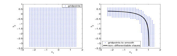
Figure 1: Example of grid points selected for the smoothing procedure in two space dimensions. We employ the smoothing operators of Kreiss et al. [13] to ensure high-order convergence of the approximations of the smoothed problem to the true solution of (18).

Figure 1 shows an example of a two-dimensional grid on the left side and on the right side a graph of the non-differentiable points of the initial condition given in (20) together with the identified grid points, where smoothing is necessary. The points are chosen in such a way that we ensure that the non-differentiable points have no influence on $\tilde{u}_{0}\left(x_{1},x_{2}\right)$ for those points, which are not shown in Figure 1 on the right hand side. This approach reduces the necessary calculations significantly. As $h\rightarrow 0$, the smooth initial condition $\tilde{u}_{0}$ converges towards the original initial condition $u_{0}$ given in (20). The results in [13] guarantee high-order convergence of the approximation of the smoothed problem to the true solution of (18).

We use the relative $l^{2}$-error $\|U_{\text{ref}}-U\|_{l^{2}}/\|U_{\text{ref}}\|_{l^{2}},$ as well as the $l^{\infty}$-error $\|U_{\text{ref}}-U\|_{l^{\infty}}$ to examine the numerical convergence rate, where $U_{\text{ref}}$ denotes a reference solution on a fine grid and $U$ is the approximation. When identifying the convergence order of the schemes, we determine it as the slope of the linear least square fit of the individual error points in the loglog-plots of error versus number of grid points per spatial direction.

9.1 Numerical example with two underlying assets

In this section we report the numerical results for a two-dimensional Black-Scholes Basket Power Put. We compare the high-order compact scheme (‘HOC’) with the standard scheme (‘2nd order’), which is obtained by using the central difference operator directly in (18) for $n=2$ with no further action and thus leads to a classical second-order scheme. We consider plain European Puts ($p=1$) and use the smoothing procedure outlined above for the initial condition (20). The parameter values

$$\sigma_{1}=0.25,\quad\sigma_{2}=0.35,\quad\gamma=0.25,\quad r=\text{ln}(1.05),\quad\omega_{1}=0.35=1-\omega_{2},\quad K=10,$$

and $\delta_{1}=\delta_{2}=0$ are used, unless stated otherwise. The parabolic mesh ratio is fixed to $\Delta\tau/h^{2}=0.4$, although we point out that neither the von Neumann stability analysis nor our numerical experiments revealed any practical restrictions on its choice.

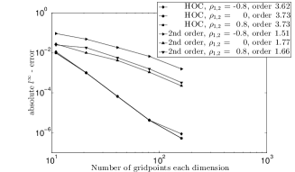
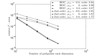
Figure 2: $l^{\infty}$- (left) and relative $l^{2}$-error (right) for two-dimensional Black-Scholes Basket Put and smoothed initial condition.

Figure 2 shows convergence plots for the $l^{\infty}$-error (left) and for the relative $l^{2}$-error (right) for a European Put, respectively. The initial condition is smoothed using the procedure outlined above. For both types of errors we observe that the numerical convergence rates agree very well with the theoretical orders of the schemes. The high-order compact scheme yields numerical convergence orders close to four and strongly outperforms the standard second-order scheme. The choice of the correlation parameter $\rho_{12}=-0.8$, $\rho_{12}=0$ and $\rho_{12}=0.8$ has very little influence.

9.2 Numerical example with three assets

In this section we report on numerical experiments with three underlying assets. We choose the parameters

$$\delta_{i}=0.01,\quad\sigma_{i}=0.3,\quad\omega_{i}=1/3,\quad r=\text{ln}(1.05),\quad\gamma=0.3,\quad T=0.25,\quad K=10.$$

Due to the computational intensity of the three-dimensional problem the number of grid points per spatial dimension is smaller compared to the results in two dimensions reported above. To ensure that at the same time there is a sufficiently large number of grid points in time, we fix the parabolic mesh ratio to $\Delta\tau/h^{2}=0.1$ (not for stability reasons). We perform two types of experiments: without any correlation between the assets (labeled by ‘nc’ in the plots), and with correlation (labeled by ‘c’ in the plots) using the parameter values $\rho_{1,2}=-0.4$, $\rho_{1,3}=-0.1$, $\rho_{2,3}=-0.2.$

We compare the standard approximation to our high-order compact scheme for European Power Put options with $p=3,4$. For the European Power Puts with $p=1,2$ one would smooth the initial condition, similar as above, to ensure high-order convergence.

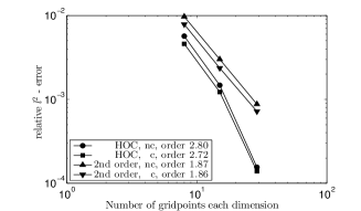
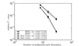
Figure 3: Relative $l^{2}$-error for three-dimensional Black-Scholes Basket Power Put, with $p=3$ (left) and $p=4$ (right)

Figure  3 shows the convergence of the relative $l^{2}$-error for a European Power Put with $p=3$ and $p=4$. We use the original initial conditions, no smoothing is applied here. The numerical convergence rates of the high-order compact scheme are slightly reduced to about three and three and a half, respectively. Additional smoothing, which we omitted here due to limit the computational load, would result in even better results. Still, in the high-order compact scheme outperforms the standard second-order scheme significantly in all cases.

9.3 Numerical example with space-dependent coefficients

In this section we will apply numerical examples for (16), where the continuous dividends are dependent on the underlying asset price. For both asset prices $S_{i}$ with $i=1,2$ we consider the following example, where the continuous dividends are zero for small asset prices and then smoothly increase around an asset price $S_{i}^{\star}>0$ towards a given parameter $\delta_{i}^{\star}\geq 0$,

$$\delta_{i}=\delta_{i}(S_{i})=\frac{\delta_{i}^{\star}\left[\tanh\left(\zeta_{i}(S_{i}-S_{i}^{\star})\right)-\tanh\left(-\zeta_{i}S_{i}^{\star}\right)\right]}{2}.$$

Financially, the interpretation could be as follows: if the asset is a dividend-paying stock, low stock prices may mean that the company may not be in the financial position to pay dividends. A low value of $\zeta_{i}>0$ leads to slow transition from $0$ to $\delta_{i}^{\star}$. We can apply the transformations given in (17) and hence use the coefficients

$$a_{i}=-\frac{\gamma^{2}}{2},\quad b_{ij}=-\gamma^{2}\rho_{ij},\quad c_{i}=\gamma\left(\frac{\sigma_{i}}{2}-\frac{r-\delta_{i}(Ke^{\frac{x_{i}\sigma_{i}}{\gamma}})}{\sigma_{i}}\right),\quad g=0,$$ (22)

for $i=1,2$ to obtain the coefficients of the numerical scheme, see Section 5.1. The boundary conditions of Section 8.4 are employed and the parameter values of Section 9.1 as well as

$$\delta_{1}^{\star}=0.02,\quad\delta_{2}^{\star}=0.01,\quad\zeta_{1}=0.35,\quad\zeta_{2}=0.5,\quad S_{i}^{\star}={0.9K}/{\omega_{i}},$$

for $i=1,2$ are used in the numerical experiments.

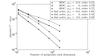
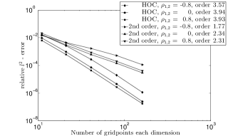
Figure 4: $l^{\infty}$- (left) and relative $l^{2}$-error (right) for two-dimensional Black-Scholes Basket Put with space-dependent dividend and smoothed initial condition.

Figure 4 shows numerical convergence plots for a European Put with space-dependent continuous dividend. Again, smoothing of the initial condition is employed. For the $l^{\infty}$-error as well as the $l^{2}$-error the high-order compact scheme has convergence rates close to four for $\rho_{1,2}=0,$ and $\rho_{1,2}=0.8$. The convergence rate for the case $\rho_{1,2}=-0.8$ is $3.22$ in the $l^{\infty}$-error, which is mainly due to the two approximations with eleven and 21 grid-points per spatial direction, and $3.57$ in the $l^{2}$-error. The convergence orders of the standard scheme are for $\rho_{1,2}=0,0.8$ are slightly above two for both types of errors. For $\rho_{1,2}=-0.8$ the convergence orders are noticeable lower as well. In all cases of correlation the high-order compact scheme outperforms the standard second-order scheme significantly.

10 Conclusion

We presented a new high-order compact scheme for a class of parabolic partial differential equations with time and space dependent coefficients, including mixed second-order derivative terms in $n$ spatial dimensions. The resulting schemes are fourth-order accurate in space and second-order accurate in time. In a thorough von Neumann stability analysis, where we focussed on the case of vanishing mixed derivative terms, we showed that a necessary stability condition holds for frozen coefficients without further conditions in two and three space dimensions. For non-vanishing mixed derivative terms we were able to give partial results. The results suggest unconditional stability of the scheme. As an application example we considered the pricing of European Power Put options in the multidimensional Black-Scholes model. The typical initial conditions of this problem lack sufficient regularity, therefore a suitable smoothing procedure was employed to ensure high-order convergence. In all numerical experiments performed a comparative standard second-order scheme is significantly outperformed.

Although we derived the scheme in arbitrary space dimension, it was not our aim in this paper to attack the so-called curse of dimensionality. The issue of exponentially increasing number of unknowns with growing spatial dimension on full grids is of course alleviated to some degree by a high-order scheme. To obtain a similar accuracy as a second-order scheme which uses $\mathcal{O}(N^{d})$ unknowns on a full grid, our high-order compact approach will ‘only’ require $\mathcal{O}(N^{d/2})$ unknowns. To really attack very high-dimensional problems one would need to combine our approach with hierarchical approaches, e.g. using sparse grids (typically requiring $\mathcal{O}(N\text{ln}(N)^{d-1})$ unknowns), which is beyond the scope of the present paper.

Appendix A Coefficients for semi-discrete scheme in three dimensions

Considering an interior grid point $\bigl{(}x_{i_{1}}^{(1)},x_{i_{2}}^{(2)},x_{i_{3}}^{(3)}\bigr{)}\in\overset{\smash{\raisebox{-0.21529pt}{$\scriptstyle\circ$}}}{G}\rule{0.0pt}{8.61108pt}_{h}^{(3)}$ and time $\tau\in\Omega_{\tau}$, the coefficients $\hat{K}_{k,l,m}$ of $U_{k,l,m}\left(\tau\right)$ for $k\in\{i_{1}-1,i_{1},i_{1}+1\}$, $l\in\{i_{2}-1,i_{2},i_{2}+1\}$ and $m\in\{i_{3}-1,i_{3},i_{3}+1\}$ of the three-dimensional semi-discrete scheme in Section 5.2 are given by:

$$\hat{K}_{i_{1},i_{2},i_{3}}= {\frac{b_{{23}}[a]_{{{{2}}}}c_{{3}}}{6{a}^{2}}}+{\frac{b_{{13}}[a]_{{{{1}}}}c_{{3}}}{6{a}^{2}}}-\frac{[c_{{3}}]_{{{{3}}}}}{3}-{\frac{{c^{2}_{{1}}}}{6a}}-{\frac{{c^{2}_{{3}}}}{6a}}-\frac{[a]_{{{11}}}}{2}-\frac{[a]_{{{22}}}}{2}-\frac{[a]_{{{33}}}}{2}+{\frac{b_{{13}}[a]_{{{{3}}}}c_{{1}}}{6{a}^{2}}}$$

$$+{\frac{b_{{12}}[a]_{{{{2}}}}c_{{1}}}{6{a}^{2}}}-{\frac{4a}{{h}^{2}}}+{\frac{b_{{13}}[a]_{{{{3}}}}[a]_{{{{1}}}}}{{a}^{2}}}+{\frac{b_{{23}}[a]_{{{{3}}}}[a]_{{{{2}}}}}{{a}^{2}}}+{\frac{b_{{23}}[a]_{{{{3}}}}c_{{2}}}{6{a}^{2}}}+{\frac{b_{{12}}[a]_{{{{1}}}}[a]_{{{{2}}}}}{{a}^{2}}}$$

$$+{\frac{b_{{12}}[a]_{{{{1}}}}c_{{2}}}{6{a}^{2}}}-{\frac{b_{{13}}[c_{{3}}]_{{{{1}}}}}{6a}}-{\frac{c_{{1}}[a]_{{{{1}}}}}{6a}}+{\frac{{b^{2}_{{23}}}}{3a{h}^{2}}}-{\frac{b_{{12}}[a]_{{{{1}}{{2}}}}}{2a}}-{\frac{c_{{2}}[a]_{{{{2}}}}}{6a}}+{\frac{{b^{2}_{{13}}}}{3a{h}^{2}}}+{\frac{{b^{2}_{{12}}}}{3a{h}^{2}}}$$

$$-{\frac{c_{{3}}[a]_{{{{3}}}}}{6a}}-{\frac{b_{{13}}[a]_{{{{1}}{{2}}}}}{2a}}-{\frac{b_{{23}}[c_{{2}}]_{{{{3}}}}}{6a}}-{\frac{b_{{12}}[c_{{2}}]_{{{{1}}}}}{6a}}-{\frac{b_{{23}}[a]_{{{{2}}{{3}}}}}{2a}}-{\frac{b_{{13}}[c_{{1}}]_{{{{3}}}}}{6a}}-{\frac{b_{{23}}[c_{{3}}]_{{{{2}}}}}{6a}}$$

$$-{\frac{b_{{12}}[c_{{1}}]_{{{{2}}}}}{6a}}-{\frac{{c^{2}_{{2}}}}{6a}}+{\frac{{[a]^{2}_{{{{1}}}}}}{a}}+{\frac{{[a]^{2}_{{{{3}}}}}}{a}}+{\frac{{[a]^{2}_{{{{2}}}}}}{a}}-\frac{[c_{{2}}]_{{{{2}}}}}{3}-\frac{[c_{{1}}]_{{{{1}}}}}{3},$$

$$\hat{K}_{i_{1}\pm 1,i_{2}-1,i_{3}}= {\frac{b_{{13}}[a]_{{{{3}}}}b_{{12}}}{24{a}^{2}h}}\mp{\frac{b_{{23}}[a]_{{{{3}}}}b_{{12}}}{24{a}^{2}h}}\mp\frac{[b_{{12}}]_{{{11}}}}{48}\mp\frac{[b_{{12}}]_{{{22}}}}{48}\mp\frac{[b_{{12}}]_{{{33}}}}{48}+{\frac{b_{{12}}[a]_{{{{1}}}}}{12ah}}-{\frac{b_{{12}}c_{{1}}}{12ah}}\pm{\frac{b_{{12}}c_{{2}}}{12ah}}$$

$$\pm{\frac{b_{{12}}[a]_{{{{1}}}}c_{{1}}}{48{a}^{2}}}\pm{\frac{b_{{12}}[a]_{{{{1}}}}[b_{{12}}]_{{{{2}}}}}{48{a}^{2}}}\mp{\frac{{b^{2}_{{12}}}[a]_{{{{1}}}}}{24{a}^{2}h}}\mp{\frac{b_{{12}}[a]_{{{{2}}}}}{12ah}}\pm{\frac{b_{{23}}[a]_{{{{2}}}}[b_{{12}}]_{{{{3}}}}}{48{a}^{2}}}\pm{\frac{b_{{13}}[a]_{{{{1}}}}[b_{{12}}]_{{{{3}}}}}{48{a}^{2}}}$$

$$\pm{\frac{b_{{12}}[a]_{{{{2}}}}[b_{{12}}]_{{{{1}}}}}{48{a}^{2}}}\pm{\frac{b_{{12}}[a]_{{{{2}}}}c_{{2}}}{48{a}^{2}}}\pm{\frac{b_{{23}}[a]_{{{{3}}}}c_{{1}}}{48{a}^{2}}}\pm{\frac{b_{{23}}[a]_{{{{3}}}}[b_{{12}}]_{{{{2}}}}}{48{a}^{2}}}-{\frac{b_{{12}}[b_{{12}}]_{{{{2}}}}}{24ah}}\pm{\frac{b_{{13}}[a]_{{{{3}}}}[b_{{12}}]_{{{{1}}}}}{48{a}^{2}}}$$

$$\pm{\frac{b_{{13}}[a]_{{{{3}}}}c_{{2}}}{48{a}^{2}}}\pm{\frac{b_{{12}}[b_{{12}}]_{{{{1}}}}}{24ah}}\pm{\frac{b_{{23}}[b_{{12}}]_{{{{3}}}}}{24ah}}-{\frac{b_{{13}}[b_{{12}}]_{{{{3}}}}}{24ah}}\pm{\frac{b_{{13}}b_{{23}}}{12a{h}^{2}}}+{\frac{[a]_{{{{2}}}}{b^{2}_{{12}}}}{24{a}^{2}h}}-{\frac{c_{{2}}}{12h}}\mp{\frac{b_{{12}}}{6{h}^{2}}}$$

$$\pm{\frac{c_{{1}}}{12h}}+{\frac{a}{6{h}^{2}}}-{\frac{[b_{{12}}]_{{{{1}}}}}{12h}}\pm{\frac{[b_{{12}}]_{{{{2}}}}}{12h}}\mp{\frac{b_{{23}}[b_{{12}}]_{{{{2}}{{3}}}}}{48a}}\mp{\frac{b_{{13}}[c_{{2}}]_{{{{3}}}}}{48a}}\mp{\frac{b_{{12}}[b_{{12}}]_{{{{1}}{{2}}}}}{48a}}\mp{\frac{b_{{23}}[c_{{1}}]_{{{{3}}}}}{48a}}$$

$$\mp{\frac{b_{{12}}[c_{{1}}]_{{{{1}}}}}{48a}}\pm{\frac{[a]_{{{{1}}}}c_{{2}}}{24a}}\mp{\frac{c_{{2}}[b_{{12}}]_{{{{2}}}}}{48a}}+{\frac{{b^{2}_{{12}}}}{12a{h}^{2}}}\mp{\frac{b_{{13}}[b_{{12}}]_{{{{1}}{{2}}}}}{48a}}\mp{\frac{c_{{1}}[b_{{12}}]_{{{{1}}}}}{48a}}\pm{\frac{[a]_{{{{3}}}}[b_{{12}}]_{{{{3}}}}}{24a}}$$

$$\mp{\frac{c_{{3}}[b_{{12}}]_{{{{3}}}}}{48a}}\pm{\frac{[a]_{{{{2}}}}c_{{1}}}{24a}}\mp{\frac{b_{{12}}[c_{{2}}]_{{{{2}}}}}{48a}}\pm{\frac{[a]_{{{{1}}}}[b_{{12}}]_{{{{1}}}}}{24a}}\pm{\frac{[a]_{{{{2}}}}[b_{{12}}]_{{{{2}}}}}{24a}}\mp{\frac{c_{{1}}c_{{2}}}{24a}}\mp\frac{[c_{{1}}]_{{{{2}}}}}{24}\mp\frac{[c_{{2}}]_{{{{1}}}}}{24},$$

$$\hat{K}_{i\pm 1,j,m}= \pm{\frac{b_{{23}}[a]_{{{{3}}}}b_{{12}}}{12{a}^{2}h}}\pm{\frac{b_{{23}}[a]_{{{{2}}}}b_{{13}}}{12{a}^{2}h}}\mp{\frac{hb_{{12}}[a]_{{{{1}}}}[c_{{1}}]_{{{{2}}}}}{24{a}^{2}}}\mp{\frac{hb_{{23}}[a]_{{{{2}}}}[c_{{1}}]_{{{{3}}}}}{24{a}^{2}}}\mp{\frac{hb_{{13}}[a]_{{{{1}}}}[c_{{1}}]_{{{{3}}}}}{24{a}^{2}}}$$

$$+{\frac{{c^{2}_{{1}}}}{12a}}\mp{\frac{hb_{{13}}[a]_{{{{3}}}}[c_{{1}}]_{{{{1}}}}}{24{a}^{2}}}\mp{\frac{hb_{{23}}[a]_{{{{3}}}}[c_{{1}}]_{{{{2}}}}}{24{a}^{2}}}\pm\frac{h[c_{{1}}]_{{{33}}}}{24}\pm\frac{h[c_{{1}}]_{{{22}}}}{24}\pm\frac{h[c_{{1}}]_{{{11}}}}{24}$$

$$+\frac{[a]_{{{11}}}}{12}+\frac{[a]_{{{22}}}}{12}+\frac{[a]_{{{33}}}}{12}-{\frac{b_{{13}}[a]_{{{{3}}}}c_{{1}}}{12{a}^{2}}}\mp{\frac{b_{{13}}[b_{{13}}]_{{{{1}}}}}{12ah}}\pm{\frac{hc_{{1}}[c_{{1}}]_{{{{1}}}}}{24a}}\pm{\frac{hc_{{2}}[c_{{1}}]_{{{{2}}}}}{24a}}$$

$$\mp{\frac{hb_{{12}}[a]_{{{{2}}}}[c_{{1}}]_{{{{1}}}}}{24{a}^{2}}}\mp{\frac{b_{{23}}[b_{{13}}]_{{{{2}}}}}{12ah}}\pm{\frac{{b^{2}_{{13}}}[a]_{{{{1}}}}}{12{a}^{2}h}}\mp{\frac{c_{{3}}b_{{13}}}{6ah}}\pm{\frac{hb_{{23}}[c_{{1}}]_{{{{2}}{{3}}}}}{24a}}\pm{\frac{hb_{{13}}[c_{{1}}]_{{{{1}}{{2}}}}}{24a}}$$

$$\pm{\frac{hb_{{12}}[c_{{1}}]_{{{{1}}{{2}}}}}{24a}}\pm{\frac{b_{{13}}[a]_{{{{3}}}}}{6ah}}-{\frac{b_{{12}}[a]_{{{{2}}}}c_{{1}}}{12{a}^{2}}}\pm{\frac{hc_{{3}}[c_{{1}}]_{{{{3}}}}}{24a}}\mp{\frac{h[a]_{{{{1}}}}[c_{{1}}]_{{{{1}}}}}{12a}}\mp{\frac{h[a]_{{{{3}}}}[c_{{1}}]_{{{{3}}}}}{12a}}$$

$$\mp{\frac{b_{{12}}c_{{2}}}{6ah}}\pm{\frac{{b^{2}_{{12}}}[a]_{{{{1}}}}}{12{a}^{2}h}}\pm{\frac{b_{{12}}[a]_{{{{2}}}}}{6ah}}\mp{\frac{b_{{12}}[b_{{12}}]_{{{{1}}}}}{12ah}}\mp{\frac{b_{{23}}[b_{{12}}]_{{{{3}}}}}{12ah}}\pm{\frac{c_{{1}}}{6h}}+{\frac{a}{3{h}^{2}}}\mp{\frac{[b_{{12}}]_{{{{2}}}}}{6h}}$$

$$-{\frac{b_{{13}}[a]_{{{{3}}}}[a]_{{{{1}}}}}{6{a}^{2}}}-{\frac{b_{{23}}[a]_{{{{3}}}}[a]_{{{{2}}}}}{6{a}^{2}}}\mp{\frac{[b_{{13}}]_{{{{3}}}}}{6h}}-{\frac{b_{{12}}[a]_{{{{1}}}}[a]_{{{{2}}}}}{6{a}^{2}}}-{\frac{c_{{1}}[a]_{{{{1}}}}}{12a}}+{\frac{b_{{12}}[a]_{{{{1}}{{2}}}}}{12a}}$$

$$+{\frac{c_{{2}}[a]_{{{{2}}}}}{12a}}-{\frac{{b^{2}_{{13}}}}{6a{h}^{2}}}-{\frac{{b^{2}_{{12}}}}{6a{h}^{2}}}+{\frac{c_{{3}}[a]_{{{{3}}}}}{12a}}+{\frac{b_{{13}}[a]_{{{{1}}{{2}}}}}{12a}}+{\frac{b_{{23}}[a]_{{{{2}}{{3}}}}}{12a}}+{\frac{b_{{13}}[c_{{1}}]_{{{{3}}}}}{12a}}$$

$$+{\frac{b_{{12}}[c_{{1}}]_{{{{2}}}}}{12a}}-{\frac{{[a]^{2}_{{{{1}}}}}}{6a}}-{\frac{{[a]^{2}_{{{{3}}}}}}{6a}}-{\frac{{[a]^{2}_{{{{2}}}}}}{6a}}+\frac{[c_{{1}}]_{{{{1}}}}}{6}\mp{\frac{h[a]_{{{{2}}}}[c_{{1}}]_{{{{2}}}}}{12a}},$$

$$\hat{K}_{i,j\pm 1,m}= \pm{\frac{b_{{13}}[a]_{{{{3}}}}b_{{12}}}{12{a}^{2}h}}\mp{\frac{hb_{{13}}[a]_{{{{1}}}}[c_{{2}}]_{{{{3}}}}}{24{a}^{2}}}\mp{\frac{hb_{{12}}[a]_{{{{1}}}}[c_{{2}}]_{{{{2}}}}}{24{a}^{2}}}\pm{\frac{b_{{13}}[a]_{{{{1}}}}b_{{23}}}{12{a}^{2}h}}\mp{\frac{hb_{{13}}[a]_{{{{3}}}}[c_{{2}}]_{{{{1}}}}}{24{a}^{2}}}$$

$$\pm{\frac{c_{{2}}}{6h}}\mp{\frac{hb_{{23}}[a]_{{{{3}}}}[c_{{2}}]_{{{{2}}}}}{24{a}^{2}}}\mp{\frac{hb_{{12}}[a]_{{{{2}}}}[c_{{2}}]_{{{{1}}}}}{24{a}^{2}}}\mp{\frac{hb_{{23}}[a]_{{{{2}}}}[c_{{2}}]_{{{{3}}}}}{24{a}^{2}}}+\frac{[a]_{{{11}}}}{12}+\frac{[a]_{{{22}}}}{12}$$

$$+\frac{[a]_{{{33}}}}{12}\pm{\frac{b_{{12}}[a]_{{{{1}}}}}{6ah}}\mp{\frac{b_{{12}}c_{{1}}}{6ah}}\mp{\frac{b_{{12}}[b_{{12}}]_{{{{2}}}}}{12ah}}\mp{\frac{b_{{13}}[b_{{12}}]_{{{{3}}}}}{12ah}}\pm{\frac{[a]_{{{{2}}}}{b^{2}_{{12}}}}{12{a}^{2}h}}+{\frac{a}{3{h}^{2}}}$$

$$\mp{\frac{[b_{{12}}]_{{{{1}}}}}{6h}}\mp{\frac{b_{{23}}c_{{3}}}{6ah}}\pm{\frac{hb_{{12}}[c_{{2}}]_{{{{1}}{{2}}}}}{24a}}\pm{\frac{hb_{{23}}[c_{{2}}]_{{{{2}}{{3}}}}}{24a}}\pm{\frac{hb_{{13}}[c_{{2}}]_{{{{1}}{{2}}}}}{24a}}-{\frac{b_{{13}}[a]_{{{{3}}}}[a]_{{{{1}}}}}{6{a}^{2}}}$$

$$\pm{\frac{hc_{{2}}[c_{{2}}]_{{{{2}}}}}{24a}}\pm{\frac{b_{{23}}[a]_{{{{3}}}}}{6ah}}-{\frac{b_{{23}}[a]_{{{{3}}}}c_{{2}}}{12{a}^{2}}}\mp{\frac{b_{{13}}[b_{{23}}]_{{{{1}}}}}{12ah}}\mp{\frac{b_{{23}}[b_{{23}}]_{{{{2}}}}}{12ah}}\mp{\frac{h[a]_{{{{2}}}}[c_{{2}}]_{{{{2}}}}}{12a}}$$

$$\pm{\frac{hc_{{3}}[c_{{2}}]_{{{{3}}}}}{24a}}\mp{\frac{h[a]_{{{{1}}}}[c_{{2}}]_{{{{1}}}}}{12a}}\mp{\frac{h[a]_{{{{3}}}}[c_{{2}}]_{{{{3}}}}}{12a}}\pm{\frac{hc_{{1}}[c_{{2}}]_{{{{1}}}}}{24a}}\pm{\frac{[a]_{{{{2}}}}{b^{2}_{{23}}}}{12{a}^{2}h}}-{\frac{b_{{12}}[a]_{{{{1}}}}[a]_{{{{2}}}}}{6{a}^{2}}}$$

$$-{\frac{b_{{12}}[a]_{{{{1}}}}c_{{2}}}{12{a}^{2}}}+{\frac{c_{{1}}[a]_{{{{1}}}}}{12a}}-{\frac{{b^{2}_{{23}}}}{6a{h}^{2}}}+{\frac{b_{{12}}[a]_{{{{1}}{{2}}}}}{12a}}-{\frac{c_{{2}}[a]_{{{{2}}}}}{12a}}-{\frac{{b^{2}_{{12}}}}{6a{h}^{2}}}+{\frac{c_{{3}}[a]_{{{{3}}}}}{12a}}$$

$$+{\frac{b_{{13}}[a]_{{{{1}}{{2}}}}}{12a}}+{\frac{b_{{23}}[c_{{2}}]_{{{{3}}}}}{12a}}+{\frac{b_{{12}}[c_{{2}}]_{{{{1}}}}}{12a}}+{\frac{b_{{23}}[a]_{{{{2}}{{3}}}}}{12a}}\pm\frac{h[c_{{2}}]_{{{22}}}}{24}\pm\frac{h[c_{{2}}]_{{{33}}}}{24}$$

$$\pm\frac{h[c_{{2}}]_{{{11}}}}{24}+{\frac{{c^{2}_{{2}}}}{12a}}-{\frac{{[a]^{2}_{{{{1}}}}}}{6a}}-{\frac{{[a]^{2}_{{{{3}}}}}}{6a}}\mp{\frac{[b_{{23}}]_{{{{3}}}}}{6h}}-{\frac{{[a]^{2}_{{{{2}}}}}}{6a}}-{\frac{b_{{23}}[a]_{{{{3}}}}[a]_{{{{2}}}}}{6{a}^{2}}}+\frac{[c_{{2}}]_{{{{2}}}}}{6},$$

$$\hat{K}_{i\pm 1,j+1,m}= -{\frac{b_{{13}}[a]_{{{{3}}}}b_{{12}}}{24{a}^{2}h}}\mp{\frac{b_{{23}}[a]_{{{{3}}}}b_{{12}}}{24{a}^{2}h}}\pm\frac{[b_{{12}}]_{{{11}}}}{48}\pm\frac{[b_{{12}}]_{{{22}}}}{48}\pm\frac{[b_{{12}}]_{{{33}}}}{48}-{\frac{b_{{12}}[a]_{{{{1}}}}}{12ah}}+{\frac{b_{{12}}c_{{1}}}{12ah}}$$

$$\pm{\frac{b_{{12}}c_{{2}}}{12ah}}\mp{\frac{b_{{12}}[a]_{{{{1}}}}c_{{1}}}{48{a}^{2}}}\mp{\frac{b_{{12}}[a]_{{{{1}}}}[b_{{12}}]_{{{{2}}}}}{48{a}^{2}}}\mp{\frac{{b^{2}_{{12}}}[a]_{{{{1}}}}}{24{a}^{2}h}}\mp{\frac{b_{{12}}[a]_{{{{2}}}}}{12ah}}\mp{\frac{b_{{23}}[a]_{{{{2}}}}[b_{{12}}]_{{{{3}}}}}{48{a}^{2}}}$$

$$\mp{\frac{b_{{13}}[a]_{{{{1}}}}[b_{{12}}]_{{{{3}}}}}{48{a}^{2}}}\mp{\frac{b_{{12}}[a]_{{{{2}}}}[b_{{12}}]_{{{{1}}}}}{48{a}^{2}}}\mp{\frac{b_{{12}}[a]_{{{{2}}}}c_{{2}}}{48{a}^{2}}}\mp{\frac{b_{{23}}[a]_{{{{3}}}}c_{{1}}}{48{a}^{2}}}\mp{\frac{b_{{23}}[a]_{{{{3}}}}[b_{{12}}]_{{{{2}}}}}{48{a}^{2}}}$$

$$+{\frac{b_{{12}}[b_{{12}}]_{{{{2}}}}}{24ah}}\mp{\frac{b_{{13}}[a]_{{{{3}}}}[b_{{12}}]_{{{{1}}}}}{48{a}^{2}}}\mp{\frac{b_{{13}}[a]_{{{{3}}}}c_{{2}}}{48{a}^{2}}}\pm{\frac{b_{{12}}[b_{{12}}]_{{{{1}}}}}{24ah}}\pm{\frac{b_{{23}}[b_{{12}}]_{{{{3}}}}}{24ah}}+{\frac{b_{{13}}[b_{{12}}]_{{{{3}}}}}{24ah}}$$

$$\mp{\frac{b_{{13}}b_{{23}}}{12a{h}^{2}}}-{\frac{[a]_{{{{2}}}}{b^{2}_{{12}}}}{24{a}^{2}h}}+{\frac{c_{{2}}}{12h}}\pm{\frac{b_{{12}}}{6{h}^{2}}}\pm{\frac{c_{{1}}}{12h}}+{\frac{a}{6{h}^{2}}}+{\frac{[b_{{12}}]_{{{{1}}}}}{12h}}\pm{\frac{[b_{{12}}]_{{{{2}}}}}{12h}}\pm{\frac{b_{{23}}[b_{{12}}]_{{{{2}}{{3}}}}}{48a}}$$

$$\pm{\frac{b_{{13}}[c_{{2}}]_{{{{3}}}}}{48a}}\pm{\frac{b_{{12}}[b_{{12}}]_{{{{1}}{{2}}}}}{48a}}\pm{\frac{b_{{23}}[c_{{1}}]_{{{{3}}}}}{48a}}\pm{\frac{b_{{12}}[c_{{1}}]_{{{{1}}}}}{48a}}\mp{\frac{[a]_{{{{1}}}}c_{{2}}}{24a}}\pm{\frac{c_{{2}}[b_{{12}}]_{{{{2}}}}}{48a}}+{\frac{{b^{2}_{{12}}}}{12a{h}^{2}}}$$

$$\pm{\frac{b_{{13}}[b_{{12}}]_{{{{1}}{{2}}}}}{48a}}\pm{\frac{c_{{1}}[b_{{12}}]_{{{{1}}}}}{48a}}\mp{\frac{[a]_{{{{3}}}}[b_{{12}}]_{{{{3}}}}}{24a}}\pm{\frac{c_{{3}}[b_{{12}}]_{{{{3}}}}}{48a}}\mp{\frac{[a]_{{{{2}}}}c_{{1}}}{24a}}\pm{\frac{b_{{12}}[c_{{2}}]_{{{{2}}}}}{48a}}$$

$$\mp{\frac{[a]_{{{{1}}}}[b_{{12}}]_{{{{1}}}}}{24a}}\mp{\frac{[a]_{{{{2}}}}[b_{{12}}]_{{{{2}}}}}{24a}}\pm{\frac{c_{{1}}c_{{2}}}{24a}}\pm\frac{[c_{{1}}]_{{{{2}}}}}{24}\pm\frac{[c_{{2}}]_{{{{1}}}}}{24},$$

$$\hat{K}_{i\pm 1,j-1,m-1}= \pm{\frac{[b_{{13}}]_{{{{2}}}}}{48h}}\mp{\frac{b_{{13}}}{24{h}^{2}}}\pm{\frac{[b_{{12}}]_{{{{3}}}}}{48h}}\pm{\frac{[b_{{23}}]_{{{{1}}}}}{48h}}\pm{\frac{b_{{12}}[b_{{13}}]_{{{{1}}}}}{96ah}}\pm{\frac{b_{{13}}[b_{{12}}]_{{{{1}}}}}{96ah}}\pm{\frac{b_{{23}}[b_{{13}}]_{{{{3}}}}}{96ah}}$$

$$\mp{\frac{b_{{23}}b_{{12}}}{24a{h}^{2}}}\mp{\frac{b_{{13}}[a]_{{{{3}}}}b_{{23}}}{48{a}^{2}h}}\mp{\frac{b_{{12}}[a]_{{{{2}}}}b_{{23}}}{48{a}^{2}h}}+{\frac{b_{{23}}}{24{h}^{2}}}\pm{\frac{b_{{13}}[b_{{23}}]_{{{{3}}}}}{96ah}}\pm{\frac{b_{{23}}c_{{1}}}{48ah}}+{\frac{b_{{12}}b_{{13}}}{24a{h}^{2}}}$$

$$\mp{\frac{b_{{12}}}{24{h}^{2}}}\mp{\frac{[a]_{{{{2}}}}b_{{13}}}{48ah}}\mp{\frac{[a]_{{{{3}}}}b_{{12}}}{48ah}}\mp{\frac{b_{{13}}[a]_{{{{1}}}}b_{{12}}}{48{a}^{2}h}}\mp{\frac{[a]_{{{{1}}}}b_{{23}}}{48ah}}\pm{\frac{b_{{12}}[b_{{23}}]_{{{{2}}}}}{96ah}}$$

$$\pm{\frac{b_{{23}}[b_{{12}}]_{{{{2}}}}}{96ah}}\pm{\frac{c_{{3}}b_{{12}}}{48ah}}\pm{\frac{b_{{13}}c_{{2}}}{48ah}}\mp{\frac{b_{{13}}b_{{23}}}{24a{h}^{2}}},$$

$$\hat{K}_{i\pm 1,j+1,m+1}= \pm{\frac{[b_{{13}}]_{{{{2}}}}}{48h}}\pm{\frac{b_{{13}}}{24{h}^{2}}}\pm{\frac{[b_{{12}}]_{{{{3}}}}}{48h}}\pm{\frac{[b_{{23}}]_{{{{1}}}}}{48h}}\pm{\frac{b_{{12}}[b_{{13}}]_{{{{1}}}}}{96ah}}\pm{\frac{b_{{13}}[b_{{12}}]_{{{{1}}}}}{96ah}}\pm{\frac{b_{{23}}[b_{{13}}]_{{{{3}}}}}{96ah}}$$

$$\pm{\frac{b_{{23}}b_{{12}}}{24a{h}^{2}}}\mp{\frac{b_{{13}}[a]_{{{{3}}}}b_{{23}}}{48{a}^{2}h}}\mp{\frac{b_{{12}}[a]_{{{{2}}}}b_{{23}}}{48{a}^{2}h}}+{\frac{b_{{23}}}{24{h}^{2}}}\pm{\frac{b_{{13}}[b_{{23}}]_{{{{3}}}}}{96ah}}\pm{\frac{b_{{23}}c_{{1}}}{48ah}}+{\frac{b_{{12}}b_{{13}}}{24a{h}^{2}}}$$

$$\pm{\frac{b_{{12}}}{24{h}^{2}}}\mp{\frac{[a]_{{{{2}}}}b_{{13}}}{48ah}}\mp{\frac{[a]_{{{{3}}}}b_{{12}}}{48ah}}\mp{\frac{b_{{13}}[a]_{{{{1}}}}b_{{12}}}{48{a}^{2}h}}\mp{\frac{[a]_{{{{1}}}}b_{{23}}}{48ah}}\pm{\frac{b_{{12}}[b_{{23}}]_{{{{2}}}}}{96ah}}$$

$$\pm{\frac{b_{{23}}[b_{{12}}]_{{{{2}}}}}{96ah}}\pm{\frac{c_{{3}}b_{{12}}}{48ah}}\pm{\frac{b_{{13}}c_{{2}}}{48ah}}\pm{\frac{b_{{13}}b_{{23}}}{24a{h}^{2}}},$$

$$\hat{K}_{i\pm 1,j,m-1}= \mp\frac{[c_{{3}}]_{{{{1}}}}}{24}\mp{\frac{b_{{13}}}{6{h}^{2}}}-{\frac{c_{{3}}}{12h}}-{\frac{[b_{{13}}]_{{{{1}}}}}{12h}}\mp{\frac{b_{{23}}[a]_{{{{2}}}}b_{{13}}}{24{a}^{2}h}}\mp\frac{[b_{{13}}]_{{{11}}}}{48}\mp\frac{[b_{{13}}]_{{{22}}}}{48}\mp\frac{[b_{{13}}]_{{{33}}}}{48}$$

$$\pm{\frac{[b_{{13}}]_{{{{3}}}}}{12h}}\pm{\frac{[a]_{{{{3}}}}[b_{{13}}]_{{{{3}}}}}{24a}}\mp{\frac{b_{{12}}[c_{{3}}]_{{{{2}}}}}{48a}}\mp{\frac{b_{{13}}[c_{{3}}]_{{{{3}}}}}{48a}}\pm{\frac{[a]_{{{{1}}}}[b_{{13}}]_{{{{1}}}}}{24a}}\mp{\frac{c_{{2}}[b_{{13}}]_{{{{2}}}}}{48a}}+{\frac{a}{6{h}^{2}}}$$

$$\pm{\frac{[a]_{{{{3}}}}c_{{1}}}{24a}}\mp{\frac{b_{{13}}[c_{{1}}]_{{{{1}}}}}{48a}}\mp{\frac{c_{{1}}[b_{{13}}]_{{{{1}}}}}{48a}}\mp{\frac{b_{{23}}[b_{{13}}]_{{{{2}}{{3}}}}}{48a}}\pm{\frac{[a]_{{{{1}}}}c_{{3}}}{24a}}\mp{\frac{c_{{1}}c_{{3}}}{24a}}\pm{\frac{[a]_{{{{2}}}}[b_{{13}}]_{{{{2}}}}}{24a}}$$

$$\mp{\frac{c_{{3}}[b_{{13}}]_{{{{3}}}}}{48a}}\mp{\frac{b_{{12}}[b_{{13}}]_{{{{1}}{{2}}}}}{48a}}\pm{\frac{b_{{13}}[b_{{13}}]_{{{{1}}}}}{24ah}}\pm{\frac{b_{{23}}[b_{{13}}]_{{{{2}}}}}{24ah}}\mp{\frac{{b^{2}_{{13}}}[a]_{{{{1}}}}}{24{a}^{2}h}}\pm{\frac{c_{{3}}b_{{13}}}{12ah}}\mp{\frac{b_{{13}}[a]_{{{{3}}}}}{12ah}}$$

$$+{\frac{b_{{12}}[a]_{{{{2}}}}b_{{13}}}{24{a}^{2}h}}\pm{\frac{c_{{1}}}{12h}}+{\frac{{b^{2}_{{13}}}}{12a{h}^{2}}}\mp{\frac{b_{{13}}[b_{{13}}]_{{{{1}}{{2}}}}}{48a}}\mp{\frac{b_{{23}}[c_{{1}}]_{{{{2}}}}}{48a}}\pm{\frac{b_{{23}}b_{{12}}}{12a{h}^{2}}}+{\frac{[a]_{{{{3}}}}{b^{2}_{{13}}}}{24{a}^{2}h}}$$

$$\pm{\frac{b_{{13}}[a]_{{{{1}}}}c_{{1}}}{48{a}^{2}}}\pm{\frac{b_{{12}}[a]_{{{{1}}}}[b_{{13}}]_{{{{2}}}}}{48{a}^{2}}}\pm{\frac{b_{{23}}[a]_{{{{2}}}}c_{{1}}}{48{a}^{2}}}\pm{\frac{b_{{13}}[a]_{{{{1}}}}[b_{{13}}]_{{{{3}}}}}{48{a}^{2}}}\pm{\frac{b_{{23}}[a]_{{{{3}}}}[b_{{13}}]_{{{{2}}}}}{48{a}^{2}}}$$

$$\pm{\frac{b_{{13}}[a]_{{{{3}}}}[b_{{13}}]_{{{{1}}}}}{48{a}^{2}}}\pm{\frac{b_{{23}}[a]_{{{{2}}}}[b_{{13}}]_{{{{3}}}}}{48{a}^{2}}}\mp\frac{[c_{{1}}]_{{{{3}}}}}{24}\pm{\frac{b_{{12}}[a]_{{{{2}}}}[b_{{13}}]_{{{{1}}}}}{48{a}^{2}}}+{\frac{b_{{13}}[a]_{{{{1}}}}}{12ah}}-{\frac{c_{{1}}b_{{13}}}{12ah}}$$

$$\pm{\frac{b_{{12}}[a]_{{{{2}}}}c_{{3}}}{48{a}^{2}}}-{\frac{b_{{13}}[b_{{13}}]_{{{{3}}}}}{24ah}}\pm{\frac{b_{{13}}[a]_{{{{3}}}}c_{{3}}}{48{a}^{2}}}-{\frac{b_{{12}}[b_{{13}}]_{{{{2}}}}}{24ah}},$$

$$\hat{K}_{i,j\pm 1,m-1}= \mp\frac{[c_{{3}}]_{{{{2}}}}}{24}\mp{\frac{b_{{23}}}{6{h}^{2}}}-{\frac{[b_{{23}}]_{{{{2}}}}}{12h}}-{\frac{c_{{3}}}{12h}}\mp{\frac{b_{{13}}[a]_{{{{1}}}}b_{{23}}}{24{a}^{2}h}}\mp\frac{[b_{{23}}]_{{{11}}}}{48}\mp\frac{[b_{{23}}]_{{{22}}}}{48}\mp\frac{[b_{{23}}]_{{{33}}}}{48}$$

$$\mp{\frac{b_{{12}}[c_{{3}}]_{{{{1}}}}}{48a}}\pm{\frac{[a]_{{{{3}}}}[b_{{23}}]_{{{{3}}}}}{24a}}\mp{\frac{b_{{23}}[c_{{2}}]_{{{{2}}}}}{48a}}\mp{\frac{b_{{23}}[c_{{3}}]_{{{{3}}}}}{48a}}\pm{\frac{[a]_{{{{2}}}}c_{{3}}}{24a}}\pm{\frac{[a]_{{{{1}}}}[b_{{23}}]_{{{{1}}}}}{24a}}\mp{\frac{c_{{2}}c_{{3}}}{24a}}$$

$$\mp{\frac{c_{{3}}[b_{{23}}]_{{{{3}}}}}{48a}}\mp{\frac{b_{{12}}[b_{{23}}]_{{{{1}}{{2}}}}}{48a}}\mp{\frac{b_{{13}}[c_{{2}}]_{{{{1}}}}}{48a}}\mp{\frac{b_{{13}}[b_{{23}}]_{{{{1}}{{2}}}}}{48a}}\pm{\frac{[a]_{{{{2}}}}[b_{{23}}]_{{{{2}}}}}{24a}}\pm{\frac{[a]_{{{{3}}}}c_{{2}}}{24a}}$$

$$+{\frac{b_{{12}}[a]_{{{{1}}}}b_{{23}}}{24{a}^{2}h}}\pm{\frac{c_{{2}}}{12h}}+{\frac{a}{6{h}^{2}}}\pm{\frac{b_{{23}}c_{{3}}}{12ah}}\mp{\frac{b_{{23}}[a]_{{{{3}}}}}{12ah}}\pm{\frac{b_{{13}}[b_{{23}}]_{{{{1}}}}}{24ah}}\pm{\frac{b_{{23}}[b_{{23}}]_{{{{2}}}}}{24ah}}+{\frac{{b^{2}_{{23}}}}{12a{h}^{2}}}$$

$$\mp{\frac{[a]_{{{{2}}}}{b^{2}_{{23}}}}{24{a}^{2}h}}\mp{\frac{b_{{23}}[b_{{23}}]_{{{{2}}{{3}}}}}{48a}}\mp{\frac{c_{{2}}[b_{{23}}]_{{{{2}}}}}{48a}}\mp{\frac{c_{{1}}[b_{{23}}]_{{{{1}}}}}{48a}}\pm{\frac{b_{{12}}b_{{13}}}{12a{h}^{2}}}-{\frac{c_{{2}}b_{{23}}}{12ah}}\pm{\frac{b_{{23}}[a]_{{{{3}}}}c_{{3}}}{48{a}^{2}}}$$

$$\pm{\frac{b_{{23}}[a]_{{{{3}}}}[b_{{23}}]_{{{{2}}}}}{48{a}^{2}}}+{\frac{b_{{23}}[a]_{{{{2}}}}}{12ah}}\pm{\frac{b_{{12}}[a]_{{{{1}}}}c_{{3}}}{48{a}^{2}}}\pm{\frac{b_{{13}}[a]_{{{{1}}}}[b_{{23}}]_{{{{3}}}}}{48{a}^{2}}}\pm{\frac{b_{{23}}[a]_{{{{2}}}}[b_{{23}}]_{{{{3}}}}}{48{a}^{2}}}$$

$$\pm{\frac{b_{{23}}[a]_{{{{2}}}}c_{{2}}}{48{a}^{2}}}\pm{\frac{b_{{12}}[a]_{{{{1}}}}[b_{{23}}]_{{{{2}}}}}{48{a}^{2}}}\pm{\frac{b_{{13}}[a]_{{{{1}}}}c_{{2}}}{48{a}^{2}}}\pm{\frac{b_{{13}}[a]_{{{{3}}}}[b_{{23}}]_{{{{1}}}}}{48{a}^{2}}}\pm{\frac{b_{{12}}[a]_{{{{2}}}}[b_{{23}}]_{{{{1}}}}}{48{a}^{2}}}$$

$$-{\frac{b_{{23}}[b_{{23}}]_{{{{3}}}}}{24ah}}-{\frac{b_{{12}}[b_{{23}}]_{{{{1}}}}}{24ah}}+{\frac{{b^{2}_{{23}}}[a]_{{{{3}}}}}{24{a}^{2}h}}\pm{\frac{[b_{{23}}]_{{{{3}}}}}{12h}}\mp\frac{[c_{{2}}]_{{{{3}}}}}{24},$$

$$\hat{K}_{i\pm 1,j+1,m-1}= \mp{\frac{[b_{{13}}]_{{{{2}}}}}{48h}}\mp{\frac{b_{{13}}}{24{h}^{2}}}\mp{\frac{[b_{{12}}]_{{{{3}}}}}{48h}}\mp{\frac{[b_{{23}}]_{{{{1}}}}}{48h}}\mp{\frac{b_{{12}}[b_{{13}}]_{{{{1}}}}}{96ah}}\mp{\frac{b_{{13}}[b_{{12}}]_{{{{1}}}}}{96ah}}\mp{\frac{b_{{23}}[b_{{13}}]_{{{{3}}}}}{96ah}}$$

$$\mp{\frac{b_{{23}}b_{{12}}}{24a{h}^{2}}}\pm{\frac{b_{{13}}[a]_{{{{3}}}}b_{{23}}}{48{a}^{2}h}}\pm{\frac{b_{{12}}[a]_{{{{2}}}}b_{{23}}}{48{a}^{2}h}}-{\frac{b_{{23}}}{24{h}^{2}}}\mp{\frac{b_{{13}}[b_{{23}}]_{{{{3}}}}}{96ah}}\mp{\frac{b_{{23}}c_{{1}}}{48ah}}-{\frac{b_{{12}}b_{{13}}}{24a{h}^{2}}}$$

$$\pm{\frac{b_{{12}}}{24{h}^{2}}}\pm{\frac{[a]_{{{{2}}}}b_{{13}}}{48ah}}\pm{\frac{[a]_{{{{3}}}}b_{{12}}}{48ah}}\pm{\frac{b_{{13}}[a]_{{{{1}}}}b_{{12}}}{48{a}^{2}h}}\pm{\frac{[a]_{{{{1}}}}b_{{23}}}{48ah}}\mp{\frac{b_{{12}}[b_{{23}}]_{{{{2}}}}}{96ah}}$$

$$\mp{\frac{b_{{23}}[b_{{12}}]_{{{{2}}}}}{96ah}}\mp{\frac{c_{{3}}b_{{12}}}{48ah}}\mp{\frac{b_{{13}}c_{{2}}}{48ah}}\pm{\frac{b_{{13}}b_{{23}}}{24a{h}^{2}}},$$

$$\hat{K}_{i\pm 1,j-1,m+1}= \mp{\frac{[b_{{13}}]_{{{{2}}}}}{48h}}\pm{\frac{b_{{13}}}{24{h}^{2}}}\mp{\frac{[b_{{12}}]_{{{{3}}}}}{48h}}\mp{\frac{[b_{{23}}]_{{{{1}}}}}{48h}}\mp{\frac{b_{{12}}[b_{{13}}]_{{{{1}}}}}{96ah}}\mp{\frac{b_{{13}}[b_{{12}}]_{{{{1}}}}}{96ah}}\mp{\frac{b_{{23}}[b_{{13}}]_{{{{3}}}}}{96ah}}$$

$$\pm{\frac{b_{{23}}b_{{12}}}{24a{h}^{2}}}\pm{\frac{b_{{13}}[a]_{{{{3}}}}b_{{23}}}{48{a}^{2}h}}\pm{\frac{b_{{12}}[a]_{{{{2}}}}b_{{23}}}{48{a}^{2}h}}-{\frac{b_{{23}}}{24{h}^{2}}}\mp{\frac{b_{{13}}[b_{{23}}]_{{{{3}}}}}{96ah}}\mp{\frac{b_{{23}}c_{{1}}}{48ah}}-{\frac{b_{{12}}b_{{13}}}{24a{h}^{2}}}$$

$$\mp{\frac{b_{{12}}}{24{h}^{2}}}\pm{\frac{[a]_{{{{2}}}}b_{{13}}}{48ah}}\pm{\frac{[a]_{{{{3}}}}b_{{12}}}{48ah}}\pm{\frac{b_{{13}}[a]_{{{{1}}}}b_{{12}}}{48{a}^{2}h}}\pm{\frac{[a]_{{{{1}}}}b_{{23}}}{48ah}}\mp{\frac{b_{{12}}[b_{{23}}]_{{{{2}}}}}{96ah}}$$

$$\mp{\frac{b_{{23}}[b_{{12}}]_{{{{2}}}}}{96ah}}\mp{\frac{c_{{3}}b_{{12}}}{48ah}}\mp{\frac{b_{{13}}c_{{2}}}{48ah}}\mp{\frac{b_{{13}}b_{{23}}}{24a{h}^{2}}},$$

$$\hat{K}_{i\pm 1,j,m+1}= \pm\frac{[c_{{3}}]_{{{{1}}}}}{24}\pm{\frac{b_{{13}}}{6{h}^{2}}}+{\frac{c_{{3}}}{12h}}+{\frac{[b_{{13}}]_{{{{1}}}}}{12h}}-\mp{\frac{b_{{23}}[a]_{{{{2}}}}b_{{13}}}{24{a}^{2}h}}\pm\frac{[b_{{13}}]_{{{11}}}}{48}\pm\frac{[b_{{13}}]_{{{22}}}}{48}\pm\frac{[b_{{13}}]_{{{33}}}}{48}$$

$$\pm{\frac{[b_{{13}}]_{{{{3}}}}}{12h}}\mp{\frac{[a]_{{{{3}}}}[b_{{13}}]_{{{{3}}}}}{24a}}\pm{\frac{b_{{12}}[c_{{3}}]_{{{{2}}}}}{48a}}\pm{\frac{b_{{13}}[c_{{3}}]_{{{{3}}}}}{48a}}\mp{\frac{[a]_{{{{1}}}}[b_{{13}}]_{{{{1}}}}}{24a}}\pm{\frac{c_{{2}}[b_{{13}}]_{{{{2}}}}}{48a}}+{\frac{a}{6{h}^{2}}}$$

$$\mp{\frac{[a]_{{{{3}}}}c_{{1}}}{24a}}\pm{\frac{b_{{13}}[c_{{1}}]_{{{{1}}}}}{48a}}\pm{\frac{c_{{1}}[b_{{13}}]_{{{{1}}}}}{48a}}\pm{\frac{b_{{23}}[b_{{13}}]_{{{{2}}{{3}}}}}{48a}}\mp{\frac{[a]_{{{{1}}}}c_{{3}}}{24a}}\pm{\frac{c_{{1}}c_{{3}}}{24a}}\mp{\frac{[a]_{{{{2}}}}[b_{{13}}]_{{{{2}}}}}{24a}}$$

$$\pm{\frac{c_{{3}}[b_{{13}}]_{{{{3}}}}}{48a}}\pm{\frac{b_{{12}}[b_{{13}}]_{{{{1}}{{2}}}}}{48a}}\pm{\frac{b_{{13}}[b_{{13}}]_{{{{1}}}}}{24ah}}\pm{\frac{b_{{23}}[b_{{13}}]_{{{{2}}}}}{24ah}}\mp{\frac{{b^{2}_{{13}}}[a]_{{{{1}}}}}{24{a}^{2}h}}\pm{\frac{c_{{3}}b_{{13}}}{12ah}}\mp{\frac{b_{{13}}[a]_{{{{3}}}}}{12ah}}$$

$$-{\frac{b_{{12}}[a]_{{{{2}}}}b_{{13}}}{24{a}^{2}h}}\pm{\frac{c_{{1}}}{12h}}+{\frac{{b^{2}_{{13}}}}{12a{h}^{2}}}\pm{\frac{b_{{13}}[b_{{13}}]_{{{{1}}{{2}}}}}{48a}}\pm{\frac{b_{{23}}[c_{{1}}]_{{{{2}}}}}{48a}}\mp{\frac{b_{{23}}b_{{12}}}{12a{h}^{2}}}-{\frac{[a]_{{{{3}}}}{b^{2}_{{13}}}}{24{a}^{2}h}}$$

$$\mp{\frac{b_{{13}}[a]_{{{{1}}}}c_{{1}}}{48{a}^{2}}}\mp{\frac{b_{{12}}[a]_{{{{1}}}}[b_{{13}}]_{{{{2}}}}}{48{a}^{2}}}\mp{\frac{b_{{23}}[a]_{{{{2}}}}c_{{1}}}{48{a}^{2}}}\mp{\frac{b_{{13}}[a]_{{{{1}}}}[b_{{13}}]_{{{{3}}}}}{48{a}^{2}}}\mp{\frac{b_{{23}}[a]_{{{{3}}}}[b_{{13}}]_{{{{2}}}}}{48{a}^{2}}}$$

$$\pm\frac{[c_{{1}}]_{{{{3}}}}}{24}\mp{\frac{b_{{13}}[a]_{{{{3}}}}[b_{{13}}]_{{{{1}}}}}{48{a}^{2}}}\mp{\frac{b_{{23}}[a]_{{{{2}}}}[b_{{13}}]_{{{{3}}}}}{48{a}^{2}}}\mp{\frac{b_{{12}}[a]_{{{{2}}}}[b_{{13}}]_{{{{1}}}}}{48{a}^{2}}}-{\frac{b_{{13}}[a]_{{{{1}}}}}{12ah}}$$

$$\mp{\frac{b_{{12}}[a]_{{{{2}}}}c_{{3}}}{48{a}^{2}}}+{\frac{b_{{13}}[b_{{13}}]_{{{{3}}}}}{24ah}}\mp{\frac{b_{{13}}[a]_{{{{3}}}}c_{{3}}}{48{a}^{2}}}+{\frac{b_{{12}}[b_{{13}}]_{{{{2}}}}}{24ah}}+{\frac{c_{{1}}b_{{13}}}{12ah}},$$

$$\hat{K}_{i,j,m\pm 1}= -{\frac{b_{{23}}[a]_{{{{2}}}}c_{{3}}}{12{a}^{2}}}-{\frac{b_{{13}}[a]_{{{{1}}}}c_{{3}}}{12{a}^{2}}}+\frac{[c_{{3}}]_{{{{3}}}}}{6}\mp{\frac{[b_{{23}}]_{{{{2}}}}}{6h}}\pm{\frac{c_{{3}}}{6h}}\mp{\frac{[b_{{13}}]_{{{{1}}}}}{6h}}\pm\frac{h[c_{{3}}]_{{{11}}}}{24}\pm\frac{h[c_{{3}}]_{{{33}}}}{24}$$

$$\pm\frac{h[c_{{3}}]_{{{22}}}}{24}+{\frac{{c^{2}_{{3}}}}{12a}}+\frac{[a]_{{{11}}}}{12}+\frac{[a]_{{{22}}}}{12}+\frac{[a]_{{{33}}}}{12}\pm{\frac{b_{{12}}[a]_{{{{1}}}}b_{{23}}}{12{a}^{2}h}}\pm{\frac{b_{{12}}[a]_{{{{2}}}}b_{{13}}}{12{a}^{2}h}}$$

$$\mp{\frac{hb_{{13}}[a]_{{{{1}}}}[c_{{3}}]_{{{{3}}}}}{24{a}^{2}}}\mp{\frac{hb_{{12}}[a]_{{{{1}}}}[c_{{3}}]_{{{{2}}}}}{24{a}^{2}}}\mp{\frac{hb_{{23}}[a]_{{{{2}}}}[c_{{3}}]_{{{{3}}}}}{24{a}^{2}}}\mp{\frac{hb_{{23}}[a]_{{{{3}}}}[c_{{3}}]_{{{{2}}}}}{24{a}^{2}}}-{\frac{b_{{13}}[a]_{{{{3}}}}[a]_{{{{1}}}}}{6{a}^{2}}}$$

$$\mp{\frac{hb_{{13}}[a]_{{{{3}}}}[c_{{3}}]_{{{{1}}}}}{24{a}^{2}}}\mp{\frac{hb_{{12}}[a]_{{{{2}}}}[c_{{3}}]_{{{{1}}}}}{24{a}^{2}}}+{\frac{a}{3{h}^{2}}}-{\frac{b_{{23}}[a]_{{{{3}}}}[a]_{{{{2}}}}}{6{a}^{2}}}-{\frac{b_{{12}}[a]_{{{{1}}}}[a]_{{{{2}}}}}{6{a}^{2}}}+{\frac{b_{{13}}[c_{{3}}]_{{{{1}}}}}{12a}}$$

$$+{\frac{c_{{1}}[a]_{{{{1}}}}}{12a}}-{\frac{{b^{2}_{{23}}}}{6a{h}^{2}}}+{\frac{b_{{12}}[a]_{{{{1}}{{2}}}}}{12a}}+{\frac{c_{{2}}[a]_{{{{2}}}}}{12a}}-{\frac{{b^{2}_{{13}}}}{6a{h}^{2}}}-{\frac{c_{{3}}[a]_{{{{3}}}}}{12a}}+{\frac{b_{{13}}[a]_{{{{1}}{{2}}}}}{12a}}\pm{\frac{hc_{{2}}[c_{{3}}]_{{{{2}}}}}{24a}}$$

$$+{\frac{b_{{23}}[a]_{{{{2}}{{3}}}}}{12a}}+{\frac{b_{{23}}[c_{{3}}]_{{{{2}}}}}{12a}}\mp{\frac{c_{{2}}b_{{23}}}{6ah}}\pm{\frac{b_{{23}}[a]_{{{{2}}}}}{6ah}}\mp{\frac{b_{{23}}[b_{{23}}]_{{{{3}}}}}{12ah}}\mp{\frac{b_{{12}}[b_{{23}}]_{{{{1}}}}}{12ah}}\pm{\frac{{b^{2}_{{23}}}[a]_{{{{3}}}}}{12{a}^{2}h}}$$

$$\pm{\frac{[a]_{{{{3}}}}{b^{2}_{{13}}}}{12{a}^{2}h}}\pm{\frac{b_{{13}}[a]_{{{{1}}}}}{6ah}}\mp{\frac{b_{{13}}[b_{{13}}]_{{{{3}}}}}{12ah}}\mp{\frac{b_{{12}}[b_{{13}}]_{{{{2}}}}}{12ah}}\mp{\frac{c_{{1}}b_{{13}}}{6ah}}\pm{\frac{hb_{{13}}[c_{{3}}]_{{{{1}}{{2}}}}}{24a}}\pm{\frac{hc_{{1}}[c_{{3}}]_{{{{1}}}}}{24a}}$$

$$\pm{\frac{hb_{{12}}[c_{{3}}]_{{{{1}}{{2}}}}}{24a}}\pm{\frac{hb_{{23}}[c_{{3}}]_{{{{2}}{{3}}}}}{24a}}\mp{\frac{h[a]_{{{{1}}}}[c_{{3}}]_{{{{1}}}}}{12a}}\mp{\frac{h[a]_{{{{2}}}}[c_{{3}}]_{{{{2}}}}}{12a}}\mp{\frac{h[a]_{{{{3}}}}[c_{{3}}]_{{{{3}}}}}{12a}}$$

$$\pm{\frac{hc_{{3}}[c_{{3}}]_{{{{3}}}}}{24a}}-{\frac{{[a]^{2}_{{{{1}}}}}}{6a}}-{\frac{{[a]^{2}_{{{{3}}}}}}{6a}}-{\frac{{[a]^{2}_{{{{2}}}}}}{6a}},$$

$$\hat{K}_{i,j\pm 1,m+1}= \pm\frac{[c_{{3}}]_{{{{2}}}}}{24}\pm{\frac{b_{{23}}}{6{h}^{2}}}+{\frac{[b_{{23}}]_{{{{2}}}}}{12h}}+{\frac{c_{{3}}}{12h}}\mp{\frac{b_{{13}}[a]_{{{{1}}}}b_{{23}}}{24{a}^{2}h}}\pm\frac{[b_{{23}}]_{{{11}}}}{48}\pm\frac{[b_{{23}}]_{{{22}}}}{48}\pm\frac{[b_{{23}}]_{{{33}}}}{48}$$

$$\pm{\frac{b_{{12}}[c_{{3}}]_{{{{1}}}}}{48a}}\mp{\frac{[a]_{{{{3}}}}[b_{{23}}]_{{{{3}}}}}{24a}}\pm{\frac{b_{{23}}[c_{{2}}]_{{{{2}}}}}{48a}}\pm{\frac{b_{{23}}[c_{{3}}]_{{{{3}}}}}{48a}}\mp{\frac{[a]_{{{{2}}}}c_{{3}}}{24a}}\mp{\frac{[a]_{{{{1}}}}[b_{{23}}]_{{{{1}}}}}{24a}}\pm{\frac{c_{{2}}c_{{3}}}{24a}}$$

$$\pm{\frac{c_{{3}}[b_{{23}}]_{{{{3}}}}}{48a}}\pm{\frac{b_{{12}}[b_{{23}}]_{{{{1}}{{2}}}}}{48a}}\pm{\frac{b_{{13}}[c_{{2}}]_{{{{1}}}}}{48a}}\pm{\frac{b_{{13}}[b_{{23}}]_{{{{1}}{{2}}}}}{48a}}\mp{\frac{[a]_{{{{2}}}}[b_{{23}}]_{{{{2}}}}}{24a}}\mp{\frac{[a]_{{{{3}}}}c_{{2}}}{24a}}$$

$$-{\frac{b_{{12}}[a]_{{{{1}}}}b_{{23}}}{24{a}^{2}h}}\pm{\frac{c_{{2}}}{12h}}+{\frac{a}{6{h}^{2}}}\pm{\frac{b_{{23}}c_{{3}}}{12ah}}\mp{\frac{b_{{23}}[a]_{{{{3}}}}}{12ah}}\pm{\frac{b_{{13}}[b_{{23}}]_{{{{1}}}}}{24ah}}\pm{\frac{b_{{23}}[b_{{23}}]_{{{{2}}}}}{24ah}}+{\frac{c_{{2}}b_{{23}}}{12ah}}$$

$$\mp{\frac{[a]_{{{{2}}}}{b^{2}_{{23}}}}{24{a}^{2}h}}+{\frac{{b^{2}_{{23}}}}{12a{h}^{2}}}\pm{\frac{b_{{23}}[b_{{23}}]_{{{{2}}{{3}}}}}{48a}}\pm{\frac{c_{{2}}[b_{{23}}]_{{{{2}}}}}{48a}}\pm{\frac{c_{{1}}[b_{{23}}]_{{{{1}}}}}{48a}}\mp{\frac{b_{{12}}b_{{13}}}{12a{h}^{2}}}-{\frac{b_{{23}}[a]_{{{{2}}}}}{12ah}}$$

$$\mp{\frac{b_{{23}}[a]_{{{{3}}}}[b_{{23}}]_{{{{2}}}}}{48{a}^{2}}}\mp{\frac{b_{{23}}[a]_{{{{3}}}}c_{{3}}}{48{a}^{2}}}\mp{\frac{b_{{12}}[a]_{{{{1}}}}c_{{3}}}{48{a}^{2}}}\mp{\frac{b_{{13}}[a]_{{{{1}}}}[b_{{23}}]_{{{{3}}}}}{48{a}^{2}}}\mp{\frac{b_{{23}}[a]_{{{{2}}}}[b_{{23}}]_{{{{3}}}}}{48{a}^{2}}}$$

$$\mp{\frac{b_{{23}}[a]_{{{{2}}}}c_{{2}}}{48{a}^{2}}}\mp{\frac{b_{{12}}[a]_{{{{1}}}}[b_{{23}}]_{{{{2}}}}}{48{a}^{2}}}\mp{\frac{b_{{13}}[a]_{{{{1}}}}c_{{2}}}{48{a}^{2}}}\mp{\frac{b_{{13}}[a]_{{{{3}}}}[b_{{23}}]_{{{{1}}}}}{48{a}^{2}}}\mp{\frac{b_{{12}}[a]_{{{{2}}}}[b_{{23}}]_{{{{1}}}}}{48{a}^{2}}}$$

$$+{\frac{b_{{23}}[b_{{23}}]_{{{{3}}}}}{24ah}}+{\frac{b_{{12}}[b_{{23}}]_{{{{1}}}}}{24ah}}-{\frac{{b^{2}_{{23}}}[a]_{{{{3}}}}}{24{a}^{2}h}}\pm{\frac{[b_{{23}}]_{{{{3}}}}}{12h}}\pm\frac{[c_{{2}}]_{{{{3}}}}}{24}.$$

Note that in the above $a,b_{12},b_{13},b_{23},c_{1},c_{2},c_{3}$ and $g$ are evaluated at $\bigl{(}x_{i_{1}}^{(1)},x_{i_{2}}^{(2)},x_{i_{3}}^{(3)}\bigr{)}\in\overset{\smash{\raisebox{-0.21529pt}{$\scriptstyle\circ$}}}{G}\rule{0.0pt}{8.61108pt}_{h}^{(3)}$ and $\tau\in\Omega_{\tau}$. To streamline the notation we used $[\cdot]_{k}$ and $[\cdot]_{kp}$ to denote the first and second derivative of the coefficients with respect to $x_{k}$, and with respect to $x_{k}$ and $x_{p}$, respectively.

References

- [1] G. Berikelashvili, M.M. Gupta, and M. Mirianashvili, Convergence of fourth order compact difference schemes for three-dimensional convection-diffusion equations, SIAM J. Numer. Anal., 45 (2007), pp. 443–455.
- [2] B. Düring and M. Fournié, High-order compact finite difference scheme for option pricing in stochastic volatility models, J. Comput. Appl. Math., 236 (2012), pp. 4462–4473.
- [3] , On the stability of a compact finite difference scheme for option pricing, in Progress in Industrial Mathematics at ECMI 2010, M. Günther and et al., eds., Berlin, Heidelberg, 2012, Springer, pp. 215–221.
- [4] B. Düring, M. Fournié, and C. Heuer, High-order compact finite difference schemes for option pricing in stochastic volatility models on non-uniform grids, J. Comput. Appl. Math., 271 (2014), pp. 247–266.
- [5] B. Düring, M. Fournié, and A. Jüngel, High-order compact finite difference schemes for a nonlinear Black-Scholes equation, Intern. J. Theor. Appl. Finance, 6 (2003), pp. 767–789.
- [6] , Convergence of a high-order compact finite difference scheme for a nonlinear Black-Scholes equation, Math. Mod. Num. Anal., 38 (2004), pp. 359–369.
- [7] M. Fournié and S. Karaa, Iterative methods and high-order difference schemes for 2D elliptic problems with mixed derivative., J. Appl. Math. Comput., 22 (2006), pp. 349–363.
- [8] M. Fournié and A. Rigal, High order compact schemes in projection methods for incompressible viscous flows, Commun. Comput. Phys., 9 (2011), pp. 994–1019.
- [9] M.M. Gupta, R.P. Manohar, and J.W. Stephenson, A single cell high order scheme for the convection-diffusion equation with variable coefficients., Int. J. Numer. Methods Fluids, 4 (1984), pp. 641–651.
- [10] , High-order difference schemes for two-dimensional elliptic equations., Numer. Methods Partial Differ. Equations, 1 (1985), pp. 71–80.
- [11] B. Gustafsson, H.-O. Kreiss, and J. Oliger, Time Dependent Problems and Difference Methods, John Wiley & Sons, New York, 2013.
- [12] S. Karaa and J. Zhang, Convergence and performance of iterative methods for solving variable coefficient convection-diffusion equation with a fourth-order compact difference scheme., Comput. Math. Appl., 44 (2002), pp. 457–479.
- [13] H.O. Kreiss, V. Thomee, and O. Widlund, Smoothing of initial data and rates of convergence for parabolic difference equations., Commun. Pure Appl. Math., 23 (1970), pp. 241–259.
- [14] S.K. Lele, Compact finite difference schemes with spectral-like resolution., J. Comput. Phys., 103 (1992), pp. 16–42.
- [15] M. Li and T. Tang, A compact fourth-order finite difference scheme for unsteady viscous incompressible flows., J. Sci. Comput., 16 (2001), pp. 29–45.
- [16] M. Li, T. Tang, and B. Fornberg, A compact fourth-order finite difference scheme for the steady incompressible Navier-Stokes equations., Int. J. Numer. Methods Fluids, 20 (1995), pp. 1137–1151.
- [17] R.D. Richtmayer and K.W. Morton, Difference Methods for Initial Value Problems, Interscience, New York, 1967.
- [18] W.F. Spotz and G.F. Carey, High-order compact scheme for the steady stream-function vorticity equations., Int. J. Numer. Methods Eng., 38 (1995), pp. 3497–3512.
- [19] , A high-order compact formulation for the 3D Poisson equation., Numer. Methods Partial Differ. Equations, 12 (1996), pp. 235–243.
- [20] , Extension of high-order compact schemes to time-dependent problems., Numer. Methods Partial Differ. Equations, 17 (2001), pp. 657–672.
- [21] J.C. Strickwerda, Finite Difference Schemes and Partial Differential Equations, SIAM, Philadelphia, 2004.
- [22] D.Y. Tangman, A. Gopaul, and M. Bhuruth, Numerical pricing of options using high-order compact finite difference schemes, J. Comp. Appl. Math., 218 (2008), pp. 270–280.
- [23] P. Wilmott, Derivatives. The theory and practice of financial engineering, John Wiley & Sons Ltd., Chichester, UK, 1998.