Non-Normal Mixtures of Experts

Abstract

Mixture of Experts (MoE) is a popular framework for modeling heterogeneity in data for regression, classification and clustering. For continuous data which we consider here in the context of regression and cluster analysis, MoE usually use normal experts, that is, expert components following the Gaussian distribution. However, for a set of data containing a group or groups of observations with asymmetric behavior, heavy tails or atypical observations, the use of normal experts may be unsuitable and can unduly affect the fit of the MoE model. In this paper, we introduce new non-normal mixture of experts (NNMoE) which can deal with these issues regarding possibly skewed, heavy-tailed data and with outliers. The proposed models are the skew-normal MoE and the robust $t$ MoE and skew $t$ MoE, respectively named SNMoE, TMoE and STMoE. We develop dedicated expectation-maximization (EM) and expectation conditional maximization (ECM) algorithms to estimate the parameters of the proposed models by monotonically maximizing the observed data log-likelihood. We describe how the presented models can be used in prediction and in model-based clustering of regression data. Numerical experiments carried out on simulated data show the effectiveness and the robustness of the proposed models in terms modeling non-linear regression functions as well as in model-based clustering. Then, to show their usefulness for practical applications, the proposed models are applied to the real-world data of tone perception for musical data analysis, and the one of temperature anomalies for the analysis of climate change data.

keywords: mixture of experts, skew normal distribution, $t$ distribution, skew $t$ distribution, EM algorithm, ECM algorithm, non-linear regression, model-based clustering

1 Introduction

Mixture of experts (MoE) introduced by (Jacobs et al., 1991) are widely studied in statistics and machine learning. They consist in a fully conditional mixture model where both the mixing proportions, known as the gating functions, and the component densities, known as the experts, are conditional on some input covariates. MoE have been investigated, in their simple form, as well as in their hierarchical form Jordan and Jacobs (1994) (e.g Section 5.12 of McLachlan and Peel. (2000)) for regression and model-based cluster and discriminant analyses and in different application domains. A complete review of the MoE models can be found in Yuksel et al. (2012). For continuous data, which we consider here in the context of non-linear regression and model-based cluster analysis, MoE usually use normal experts, that is, expert components following the Gaussian distribution. Along this paper, We will call it the normal mixture of experts, abbreviated as NMoE. However, it is well-known that the normal distribution is sensitive to outliers. Moreover, for a set of data containing a group or groups of observations with heavy tails or asymmetric behavior, the use of normal experts may be unsuitable and can unduly affect the fit of the MoE model. In this paper, we attempt to overcome these limitations in MoE by proposing more adapted and robust mixture of experts models which can deal with possibly skewed, heavy-tailed and atypical data.

Recently, the problem of sensitivity of NMoE to outliers have been considered by Nguyen and McLachlan (2014) where the authors proposed a Laplace mixture of linear experts (LMoLE) for a robust modeling of non-linear regression data. The model parameters are estimated by maximizing the observed-data likelihood via a minorization-maximization (MM) algorithm. Here, we propose alternative MoE models, by relaying on other non-normal distributions that generalize the normal distribution, that is, the skew-normal, $t$, and the skew-$t$ distributions. We call these proposed NNMoE models, respectively, the skew-normal MoE (SNMoE), the $t$ MoE (TMoE), and the skew-$t$ MoE (STMoE). Indeed, in these last years, the use of the skew normal distribution, firstly proposed by Azzalini (1985, 1986), has been shown beneficial in dealing with asymmetric data in various theoretic and applied problems. This has been studied in the finite mixture literature by namely Lin et al. (2007b) for modeling asymmetric univariate data with the univariate skew-normal mixture. On the other hand, the $t$ distribution provides a natural robust extension of the normal distribution to model data with possible outliers. This has been integrated to develop the $t$ mixture model proposed by Mclachlan and Peel (1998) for robust cluster analysis of multivariate data. Recently, Bai et al. (2012) proposed a robust mixture modeling in the regression context on univariate data, by using a univariate $t$-mixture model. Moreover, in many practical problems, the robustness of $t$ mixtures may however be not sufficient in the presence of asymmetric observations. To deal with this issue, Lin et al. (2007a) proposed the univariate skew-$t$ mixture model which allows for accommodation of both skewness and thick tails in the data, by relying on the skew-$t$ distribution, introduced by Azzalini and Capitanio (2003). For the general multivariate case using $t$, skew-normal and skew-$t$ mixtures, one can refer to Mclachlan and Peel (1998); Peel and Mclachlan (2000), Pyne et al. (2009), (Lin, 2010), Lee and McLachlan (2013b), Lee and McLachlan (2013a), Lee and McLachlan (2014), and recently, the unifying framework for previous restricted and unrestricted skew-$t$ mixtures, using the CFUST distribution Lee and McLachlan (2015). The inference in the previously described approaches is performed by maximum likelihood estimation via expectation-maximization (EM) or extensions (Dempster et al., 1977; McLachlan and Krishnan, 2008), in particular the expectation conditional maximization (ECM) algorithm (Meng and Rubin, 1993). For the Bayesian framework, Frühwirth-Schnatter and Pyne (2010) have considered the Bayesian inference for both the univariate and the multivariate skew-normal and skew-$t$ mixtures. For the regression context, the robust modeling of regression data has been studied namely by Wei (2012) who considered a $t$-mixture model for regression analysis of univariate data, as well as by Bai et al. (2012) who relied on the M-estimate in mixture of linear regressions. In the same context of regression, Song et al. (2014) proposed the mixture of Laplace regressions, which has been then extended by Nguyen and McLachlan (2014) to the case of mixture of experts, by introducing the Laplace mixture of linear experts (LMoLE). Recently, Zeller et al. (2015) introduced the scale mixtures of skew-normal distributions for robust mixture regressions. However, unlike our proposed NNMoE models, the regression mixture models of Wei (2012), Bai et al. (2012), Song et al. (2014), Zeller et al. (2015) do not consider conditional mixing proportions, that is, mixing proportions depending on some input variables, as in the case of mixture of experts, which we investigate here. In addition, the approaches of Wei (2012), Bai et al. (2012) and Song et al. (2014) do not consider both the problem of robustness to outliers and the one to deal with possibly asymmetric data. Indeed, here we consider the mixture of experts framework for non-linear regression problems and model-based clustering of regression data, and we attempt to overcome the limitations of the NMoE model for dealing with asymmetric, heavy-tailed data and which may contain outliers. We investigate the use of the skew-normal, $t$ and skew $t$ distributions for the experts, rather than the commonly used normal distribution. First, the skew-normal mixture of experts (SNMoE) is proposed to accommodate data with possible asymmetric behavior. For heavy tailed or possibly noisy data, that is, data with atypical observations, we first propose the $t$-mixture of experts model (TMoE) to handle the issues regarding namely the sensitivity of the NMoE to outliers. Finally, we propose the skew-$t$ mixture of experts model (STMoE) which allows for accommodation of both skewness and heavy tails in the data and which is also robust to outliers. These models correspond to extensions of the unconditional mixture of skew-normal (Lin et al., 2007b), $t$ (Mclachlan and Peel, 1998; Wei, 2012), and skew $t$ (Lin et al., 2007a) models, to the mixture of experts (MoE) framework, where the mixture means are regression functions and the mixing proportions are covariate-varying. For the models inference, we develop dedicated expectation-maximization (EM) and expectation conditional maximization (ECM) algorithms to estimate the parameters of the proposed models by monotonically maximizing the observed data log-likelihood. The EM algorithms are indeed very popular and successful estimation algorithms for mixture models in general and for mixture of experts in particular. Moreover, the EM algorithm for MoE has been shown by Ng and McLachlan (2004) to be monotonically maximizing the MoE likelihood. The authors have showed that the EM (with IRLS in this case) algorithm has stable convergence and the log-likelihood is monotonically increasing when a learning rate smaller than one is adopted for the IRLS procedure within the M-step of the EM algorithm. They have further proposed an expectation conditional maximization (ECM) algorithm to train MoE, which also has desirable numerical properties. The MoE has also been considered in the Bayesian framework, for example one can cite the Bayesian MoE Waterhouse et al. (1996); Waterhouse (1997) and the Bayesian hierarchical MoE Bishop and Svensén (2003). Beyond the Bayesian parametric framework, the MoE models have also been investigated within the Bayesian non-parametric framework. We cite for example the Bayesian non-parametric MoE model (Rasmussen and Ghahramani, 2001) and the Bayesian non-parametric hierarchical MoE approach of J. Q. Shi and Titterington (2005) using Gaussian Processes experts for regression. For further models on mixture of experts for regression, the reader can be referred to for example the book of Shi and Choi (2011). In this paper, we investigate semi-parametric models under the maximum likelihood estimation framework.

The remainder of this paper is organized as follows. In Section 2 we briefly recall the MoE framework, the NMoE model and its maximum-likelihood estimation via EM. In Section 3, we present the SNMoE model and in Section 4 we present its inference technique using the ECM algorithm. Then, in Section 5 we present the TMoE model and derive its parameter estimation technique using the EM algorithm in Section 6. Then, in Section 7, we present the STMoE model and in Section 8 the parameter estimation technique using the ECM algorithm. In Section 11, we also show how the model selection can be performed for these NNMoE models. We then investigate in Section 9 the use of the proposed models for fitting non-linear regression functions as well for prediction on future data. We also show in Section 10 how the models can be used in a model-based clustering prospective. In Section 12, we perform experiments to assess the proposed models. Finally, in Section 13, conclusions are drawn and a future work

2 Mixture of experts for continuous data

Mixture of experts (Jacobs et al., 1991; Jordan and Jacobs, 1994) are used in a variety of contexts including regression, classification and clustering. Here we consider the MoE framework for fitting (non-linear) regression functions and clustering of univariate continuous data . The aim of regression is to explore the relationship of an observed random variable $Y$ given a covariate vector $\boldsymbol{X}\in\mathbb{R}^{p}$ via conditional density functions for $Y|\boldsymbol{X}=\boldsymbol{x}$ of the form $f(y|\boldsymbol{x})$, rather than only exploring the unconditional distribution of $Y$. For their reach modeling flexibility, mixture models (McLachlan and Peel., 2000) has took much attention for non-linear regression problems and we distinguish in particular mixture of regressions and mixture of experts for regression analysis. The univariate mixture of regressions model assumes that the observed pairs of data $(\boldsymbol{x},y)$ where $y\in\mathbb{R}$ is the response for some covariate $\boldsymbol{x}\in\mathbb{R}^{p}$, are generated from $K$ regression functions and are governed by a hidden categorical random variable $Z$ indicating from which component each observation is generated. Thus, the mixture of regressions model decomposes the nonlinear regression model density $f(y|\boldsymbol{x})$ into a convex weighted sum of $K$ regression component models $f_{k}(y|\boldsymbol{x})$ and can be defined as follows:

$$f(y|\boldsymbol{x};\boldsymbol{\varPsi}) = \sum_{k=1}^{K}\pi_{k}f_{k}(y|\boldsymbol{x};\boldsymbol{\varPsi}_{k})$$ (1)

where the $\pi_{k}$’s are defined by $\pi_{k}=\mathbb{P}(Z=k)$ and represent the non-negative mixing proportions that sum to 1. The model parameter vector is given by $\boldsymbol{\varPsi}=(\pi_{1},\ldots,\pi_{K-1},\boldsymbol{\varPsi}^{T}_{1},\ldots,\boldsymbol{\varPsi}^{T}_{K})^{T}$, $\boldsymbol{\varPsi}_{k}$ being the parameter vector of the $k$th component density.

Although similar, the mixture of experts (Jacobs et al., 1991) differ from regression mixture models in many aspects. One of the main differences is that the MoE model consists in a fully conditional mixture while in the regression mixture, only the component densities are conditional. Indeed, the mixing proportions are constant for the regression mixture, while in the MoE, they are modeled as a function of the inputs, generally modeled by logistic or a softmax function.

2.1 The mixture of experts (MoE) model

Mixture of experts (MoE) for regression analysis (Jacobs et al., 1991; Jordan and Jacobs, 1994) extend the model (1) by modeling the mixing proportions as function of some covariates $\boldsymbol{r}\in\mathbb{R}^{q}$. The mixing proportions, known as the gating functions in the context of MoE, are modeled by the multinomial logistic model and are defined by:

$$\mathbb{P}(Z=k|\boldsymbol{r};\boldsymbol{\alpha}) = \frac{\exp{(\boldsymbol{\alpha}_{k}^{T}\boldsymbol{r})}}{\sum_{\ell=1}^{K}\exp{(\boldsymbol{\alpha}_{\ell}^{T}\boldsymbol{r})}}$$ (2)

$$= \pi_{k}(\boldsymbol{r};\boldsymbol{\alpha})$$

where $\boldsymbol{r}\in\mathbb{R}^{q}$ is a covariate vector, $\boldsymbol{\alpha}_{k}$ is the $q$-dimensional coefficients vector associated with $\boldsymbol{r}$ and $\boldsymbol{\alpha}=(\boldsymbol{\alpha}^{T}_{1},\ldots,\boldsymbol{\alpha}^{T}_{K-1})^{T}$ is the parameter vector of the logistic model, with $\boldsymbol{\alpha}_{K}$ being the null vector. Thus, the MoE model consists in a fully conditional mixture model where both the mixing proportions (the gating functions) and the component densities (the experts) are conditional on some covariate variables (respectively $\boldsymbol{r}$ and $\boldsymbol{x}$). The use of mixtures with mixing proportions defined through a logistic regression model has also been studied by Huang et al. (2015) for penalized model-based clustering of spatial data by using a mixture of offset-normal shape factor analyzers (MOSFA).

2.2 The normal mixture of experts (NMoE) model and its maximum likelihood estimation

In the case of mixture of experts for regression, it is usually assumed that the experts are normal, that is, follow a normal distribution. A $K$-component normal mixture of experts (NMoE) ($K>1$) has the following formulation:

$$f(y|\boldsymbol{r},\boldsymbol{x};\boldsymbol{\varPsi}) = \sum_{k=1}^{K}\pi_{k}(\boldsymbol{r};\boldsymbol{\alpha})\text{N}\left(y;\mu(\boldsymbol{x};\boldsymbol{\beta}_{k}),\sigma_{k}^{2}\right)$$ (3)

which involves, in the semi-parametric case, component means defined as parametric (non-)linear regression functions $\mu(\boldsymbol{x};\boldsymbol{\beta}_{k})$.

The NMoE model parameters are estimated by maximizing the observed data log-likelihood by using the EM algorithm (Dempster et al., 1977; Jacobs et al., 1991; Jordan and Jacobs, 1994; Jordan and Xu, 1995; Ng and McLachlan, 2004; McLachlan and Krishnan, 2008). Suppose we observe an i.i.d sample of $n$ observations $(y_{1},\ldots,y_{n})$ with their respective associated covariates $(\boldsymbol{x}_{1},\ldots,\boldsymbol{x}_{n})$ and $(\boldsymbol{r}_{1},\ldots,\boldsymbol{x}_{r})$. Then under the MoE model, the observed data log-likelihood for the parameter vector $\boldsymbol{\varPsi}$ is given by:

$$\log L(\boldsymbol{\varPsi})=\sum_{i=1}^{n}\log\sum_{k=1}^{K}\pi_{k}(\boldsymbol{r}_{i};\boldsymbol{\alpha})\text{N}\left(y_{i};\mu(\boldsymbol{x};\boldsymbol{\beta}_{k}),\sigma_{k}^{2}\right).$$ (4)

The E-Step at the $m$th iteration of the EM algorithm for the NMoE model requires the calculation of the following posterior probability that the observation $(y_{i},\boldsymbol{x}_{i},\boldsymbol{r}_{i})$ belongs to expert $k$, given a parameter estimation $\boldsymbol{\varPsi}^{(m)}$:

$$\tau_{ik}^{(m)}=\mathbb{P}(Z_{i}=k|y_{i},\boldsymbol{x}_{i},\boldsymbol{r}_{i};\boldsymbol{\varPsi}^{(m)})=\frac{\pi_{k}(\boldsymbol{r};\boldsymbol{\alpha}^{(m)})\text{N}\left(y_{i};\mu_{k}(\boldsymbol{x}_{i};\beta^{(m)}_{k}),{\sigma^{2}_{k}}^{(m)}\right)}{f(y_{i};\boldsymbol{\varPsi}^{(m)})}.$$ (5)

Then, the M-step calculates the parameter update $\boldsymbol{\varPsi}^{(m+1)}$ by maximizing the well-known $Q$-function, that is the expected complete-data log-likelihood:

$$\boldsymbol{\varPsi}^{(m+1)}=\arg\max_{\boldsymbol{\varPsi}\in\boldsymbol{\Omega}}Q(\boldsymbol{\varPsi};\boldsymbol{\varPsi}^{(m)})$$ (6)

where $\boldsymbol{\Omega}$ is the parameter space. For example, in the case of normal mixture of linear experts (NMoLE) where each expert’s mean has the flowing linear form:

$$\mu(\boldsymbol{x};\boldsymbol{\beta}_{k})=\boldsymbol{\beta}_{k}^{T}\boldsymbol{x},$$ (7)

where $\boldsymbol{\beta}_{k}\in\mathbb{R}^{p}$ is the vector of regression coefficients of component $k$, the updates for each of the expert component parameters consist in analytically solving a weighted Gaussian linear regression problem and are given by:

$$\boldsymbol{\beta}_{k}^{(m+1)} = \Big{[}\sum_{i=1}^{n}\tau^{(m)}_{ik}\boldsymbol{x}_{i}\boldsymbol{x}^{T}_{i}\Big{]}^{-1}\sum_{i=1}^{n}\tau^{(q)}_{ik}y_{i}\boldsymbol{x}_{i},$$ (8)

$${\sigma^{2}_{k}}^{(m+1)} = \frac{\sum_{i=1}^{n}\tau_{ik}^{(m)}\left(y_{i}-{\boldsymbol{\beta}^{T}_{k}}^{(m+1)}\boldsymbol{x}_{i}\right)^{2}}{\sum_{i=1}^{n}\tau_{ik}^{(m)}}\cdot$$ (9)

For the mixing proportions, the parameter update $\boldsymbol{\alpha}^{(m+1)}$ cannot however be obtained in a closed form. It is calculated by Iteratively Reweighted Least Squares (IRLS) (Jacobs et al., 1991; Jordan and Jacobs, 1994; Chen et al., 1999; Green, 1984; Chamroukhi et al., 2009a; Chamroukhi, 2010).

However, the normal distribution is not adapted to deal with asymmetric and heavy tailed data. It is also known that the normal distribution is sensitive to outliers. In the proposal, we first propose to address the issue regarding the skewness, by proposing the skew-normal mixture of experts (SNMoE). Then, we propose a robust fitting of the MoE, which is adapted to heavy-tailed data, by using the $t$ distribution, that is, the $t$ mixture of experts (TMoE). Finally, the proposed skew-$t$ mixture of experts (STMoE) allows for simultaneously accommodating asymmetry and heavy tails in the data and is also robust to outliers.

3 The skew-normal mixture of experts (SNMoE) model

The skew-normal mixture of experts (SNMoE) model uses the skew-normal distribution as density for the expert components. We first recal the skew-normal distribution and describe its stochastic and hierarchical presentation, to then integrate them into the proposed SNMoE model.

3.1 The skew-normal distribution

As introduced by (Azzalini, 1985, 1986), a random variable $Y$ follows a univariate skew-normal distribution with location parameter $\mu\in\mathbb{R}$, scale parameter $\sigma^{2}\in(0,\infty)$ and skewness parameter $\lambda\in\mathbb{R}$ if it has the density

$$f(y;\mu,\sigma^{2},\lambda) = \frac{2}{\sigma}\phi(\frac{y-\mu}{\sigma})\Phi\left(\lambda(\frac{y-\mu}{\sigma})\right)$$ (10)

where $\phi(.)$ and $\Phi(.)$ denote, respectively, the probability density function (pdf) and the cumulative distribution function (cdf) of the standard normal distribution. It can be seen from (10) that when $\lambda=0$, the skew-normal reduces to the normal distribution. As presented by Azzalini (1986); Henze (1986), if

$$Y=\mu+\delta|U|+\sqrt{1-\delta^{2}}E$$ (11)

where $\delta=\frac{\lambda}{\sqrt{1+\lambda^{2}}}$, $U$ and $E$ are independent random variables following the normal distribution $\text{N}(0,\sigma^{2})$, then $Y$ follows the skew-normal distribution with pdf $\text{SN}(\mu,\sigma^{2},\lambda)$ given by (10). In the above, $|U|$ denotes the magnitude of $U$. This stochastic representation of the skew-normal distribution leads to the following hierarchical representation in an incomplete data framework, as presented in Lin et al. (2007b):

$$Y|u$$

.

(12)

This hierarchical representation greatly facilitates the inference for the model, namely in the skew-normal mixture model. Introduced by Lin et al. (2007b), a $K$-component skew-normal mixture model is given by:

$$f(y;\boldsymbol{\varPsi}) = \sum_{k=1}^{K}\pi_{k}\leavevmode\nobreak\ \text{SN}(y;\mu_{k},\sigma_{k}^{2},\lambda_{k})$$ (13)

where the mixture components have a skew-normal density $\text{SN}(.;.,.,.)$ given by (10). For the skew-normal mixture, the mixing proportions and the means of the mixture components are assumed to be constant.

In the following section, we present the skew-normal mixture of experts (SNMoE) which extends the skew-normal mixture model to the case of mixture of experts framework, by considering conditional distributions for both the mixing proportions and the means of the mixture components.

3.2 The skew-normal mixture of experts (SNMoE)

The proposed skew-normal MoE (SNMoE) is a $K$-component MoE model with skew-normal experts. It is defined as follows. Let $\text{SN}(\mu,\sigma^{2},\lambda)$ denotes a skew-normal distribution with location parameter $\mu$, scale parameter $\sigma$ and skewness parameter $\lambda$. A $K$-component SNMoE is then defined by:

$$f(y|\boldsymbol{r},\boldsymbol{x};\boldsymbol{\varPsi}) = \sum_{k=1}^{K}\pi_{k}(\boldsymbol{r};\boldsymbol{\alpha})\text{SN}\!\left(y;\mu(\boldsymbol{x};\boldsymbol{\beta}_{k}),\sigma_{k}^{2},\lambda_{k}\right).$$ (14)

In the SNMoE model, each expert component $k$ has indeed a skew-normal distribution, whose density is defined by (10). The parameter vector of the model is $\boldsymbol{\varPsi}=(\boldsymbol{\alpha}^{T}_{1},\ldots,\boldsymbol{\alpha}^{T}_{K-1},\boldsymbol{\varPsi}^{T}_{1},\ldots,\boldsymbol{\varPsi}^{T}_{K})^{T}$ with $\boldsymbol{\varPsi}_{k}=(\boldsymbol{\beta}^{T}_{k},\sigma^{2}_{k},\lambda_{k})^{T}$ the parameter vector for the $k$th skewed-normal expert component. It is obvious to see that if the skewness parameter $\lambda_{k}=0$ for each $k$, the SNMoE model (14) reduces to the NMoE model (3). Before going on the model inference, we first present its stochastic and hierarchical representations, which will serve to derive the ECM algorithm for maximum likelihood parameter estimation. The SNMoE model is characterized as follows.

3.2.1 Stochastic representation of the SNMoE

By using the stochastic representation (11) of the skew-normal distribution, the stochastic representation for the skew-normal mixture of experts (SNMoE) is as follows. Let $U$ and $E$ be independent univariate random variables following the standard normal distribution $\text{N}(0,1)$ with pdf $\phi(.)$. Given some covariates $\boldsymbol{x}_{i}$ and $\boldsymbol{r}_{i}$, a random variable $Y_{i}$ is said to follow the SNMoE model (14) if it has the following representation:

$$Y_{i}=\mu(\boldsymbol{x}_{i};\boldsymbol{\beta}_{z_{i}})+\delta_{z_{i}}\sigma_{z_{i}}|U_{i}|+\sqrt{1-\delta_{z_{i}}^{2}}\,\sigma_{z_{i}}E_{i}.$$ (15)

In (15), we have $\delta_{z_{i}}=\frac{\lambda_{z_{i}}}{\sqrt{1+\lambda_{z_{i}}^{2}}}$ where $z_{i}\in\{1,\ldots,K\}$ is a realization of the categorical variable $Z_{i}$ which follows the multinomial distribution, that is:

$$Z_{i}|\boldsymbol{r}_{i}\sim\text{Mult}\!\left(1;\pi_{1}(\boldsymbol{r}_{i};\boldsymbol{\alpha}),\ldots,\pi_{K}(\boldsymbol{r}_{i};\boldsymbol{\alpha})\right)$$ (16)

where each of the probabilities $\pi_{z_{i}}(\boldsymbol{r}_{i};\boldsymbol{\alpha})=\mathbb{P}(Z_{i}=z_{i}|\boldsymbol{r}_{i})$ is given by the logistic function (2). In this incomplete data framework, $z_{i}$ represents the hidden label of the component generating the $i$th observation.

The stochastic representation (15) of the SNMoE leads to the following hierarchical representation, which, as it will be presented in Section 4, greatly facilitates the model inference.

3.2.2 Hierarchical representation of the SNMoE

By introducing the binary latent component-indicators $Z_{ik}$ such that $Z_{ik}=1$ iff $Z_{i}=k$, $Z_{i}$ being the hidden class label of the $i$th observation, a hierarchical model for the SNMoE model can be derived from its stochastic representation (15) and is as follows

$$Y_{i}|u_{i},Z_{ik}=1,\boldsymbol{x}_{i} \sim \text{N}\Big{(}\mu(\boldsymbol{x}_{i};\boldsymbol{\beta}_{k})+\delta_{k}|u_{i}|,(1-\delta^{2}_{k})\sigma^{2}_{k}\Big{)},$$

$$U_{i}|Z_{ik}=1 \sim \text{N}(0,\sigma^{2}_{k}),$$ (17)

$$\boldsymbol{Z}_{i}|\boldsymbol{r}_{i} \sim \text{Mult}\left(1;\pi_{1}(\boldsymbol{r}_{i};\boldsymbol{\alpha}),\ldots,\pi_{K}(\boldsymbol{r}_{i};\boldsymbol{\alpha})\right)$$

where $\boldsymbol{Z}_{i}=(Z_{i1},\ldots,Z_{iK})$ and $\delta_{k}=\frac{\lambda_{k}}{\sqrt{1+\lambda^{2}_{k}}}$.

4 Maximum likelihood estimation of the SNMoE model

The unknown parameter vector $\boldsymbol{\varPsi}$ of the SNMoE model can be estimated by maximizing the observed-data log-likelihood. Given an observed i.i.d sample of $n$ observations $(y_{1},\ldots,y_{n})$ with their respective associated covariates $(\boldsymbol{x}_{1},\ldots,\boldsymbol{x}_{n})$ and $(\boldsymbol{r}_{1},\ldots,\boldsymbol{x}_{r})$, under the SNMoE model (14), the observed data log-likelihood for the parameter vector $\boldsymbol{\varPsi}$ is given by:

$$\log L(\boldsymbol{\varPsi})=\sum_{i=1}^{n}\log\sum_{k=1}^{K}\pi_{k}(\boldsymbol{r}_{i};\boldsymbol{\alpha})\text{SN}\left(y;\mu(\boldsymbol{x};\boldsymbol{\beta}_{k}),\sigma_{k}^{2},\lambda_{k}\right).$$ (18)

The maximization of this log-likelihood can not be performed in a closed form. However, in this latent data framework, the maximization can be performed via expectation-maximization (EM)-type algorithms (McLachlan and Krishnan, 2008). More specifically, we propose a dedicated Expectation Conditional Maximization (ECM) algorithm to monotonically maximize (18). The ECM algorithm (Meng and Rubin, 1993) is an EM variant that mainly aims at addressing the optimization problem in the M-step of the EM algorithm. In ECM, the M-step is performed by several conditional maximization (CM) steps by dividing the parameter space into sub-spaces. The parameter vector updates are then performed sequentially, one coordinate block after another in each sub-space.

4.1 ECM-algorithm for the SNMoE model

Deriving the ECM algorithm requires the definition of the complete-data log-likelihood. From the hierarchical representation (17) of the SNMoE, the complete-data log-likelihood $\boldsymbol{\varPsi}$, where the complete-data are $\{y_{i},z_{i},u_{i},\boldsymbol{x}_{i},\boldsymbol{r}_{i}\}_{i=1}^{n}$, is given by:

$$\log L_{c}(\boldsymbol{\varPsi}) \!\!=\!\! \sum_{i=1}^{n}\sum_{k=1}^{K}Z_{ik}\big{[}\log\left(\mathbb{P}\left(Z_{i}=k|\boldsymbol{r}_{i}\right)\right)+\log\left(f\left(u_{i}|Z_{ik}=1\right)\right)+\log\left(f\left(y_{i}|u_{i},Z_{ik}=1,\boldsymbol{x}_{i}\right)\right)\big{]}$$ (19)

$$= \log L_{c}(\boldsymbol{\alpha})+\sum_{k=1}^{K}\log L_{c}(\boldsymbol{\varPsi}_{k}),$$

with

$$\log L_{c}(\boldsymbol{\alpha}) \!\!=\!\! \sum_{i=1}^{n}\sum_{k=1}^{K}Z_{ik}\log\pi_{k}(\boldsymbol{r}_{i};\boldsymbol{\alpha}),$$

$$\log L_{c}(\boldsymbol{\varPsi}_{k}) \!\!=\!\! \sum_{i=1}^{n}Z_{ik}\Big{[}-\log(2\pi)-\log(\sigma^{2}_{k})-\frac{1}{2}\log(1-\delta^{2}_{k})-\frac{d^{2}_{ik}}{2(1-\delta^{2}_{k})}+\frac{\delta_{k}\leavevmode\nobreak\ d_{ik}\leavevmode\nobreak\ u_{i}}{(1-\delta^{2}_{k})\sigma_{k}}-\frac{u_{i}^{2}}{2(1-\delta^{2}_{k})\sigma^{2}_{k}}\Big{]},$$

where $d_{ik}=\frac{y_{i}-\mu(\boldsymbol{x}_{i};\boldsymbol{\beta}_{k})}{\sigma_{k}}$ denotes the Mahalanobis distance between $y_{i}$ and the $k$th expert’s mean (with $\sigma_{k}$ as the standard deviation). Then, the proposed ECM algorithm for the SNMoE model performs as follows. It starts with an initial parameter vector $\boldsymbol{\varPsi}^{(0)}$ and alternates between the E- and CM- steps until a convergence criterion is satisfied.

4.1.1 E-Step

The E-Step of the ECM algorithm for the SNMoE calculates the $Q$-function, that is the conditional expectation of the complete-data log-likelihood (19), given the observed data $\{(y_{i},\boldsymbol{x}_{i},\boldsymbol{r}_{i})\}_{i=1}^{n}$ and a current parameter estimation $\boldsymbol{\varPsi}^{(m)}$, $m$ being the current iteration:

$$Q(\boldsymbol{\varPsi};\boldsymbol{\varPsi}^{(m)}) = \mathbb{E}\big{[}\log L_{c}(\boldsymbol{\varPsi})|\{y_{i},\boldsymbol{x}_{i},\boldsymbol{r}_{i}\}_{i=1}^{n};\boldsymbol{\varPsi}^{(m)}\big{]}.$$ (20)

From (19), it follows that the $Q$-function is given by:

$$Q(\boldsymbol{\varPsi};\boldsymbol{\varPsi}^{(m)})=Q_{1}(\boldsymbol{\alpha};\boldsymbol{\varPsi}^{(m)})+\sum_{k=1}^{K}Q_{2}(\boldsymbol{\varPsi}_{k};\boldsymbol{\varPsi}^{(m)}),$$ (21)

with

$$Q_{1}(\boldsymbol{\alpha};\boldsymbol{\varPsi}^{(m)}) = \sum_{i=1}^{n}\sum_{k=1}^{K}\tau^{(m)}_{ik}\log\pi_{k}(\boldsymbol{r}_{i};\boldsymbol{\alpha}),$$ (22)

$$Q_{2}(\boldsymbol{\varPsi}_{k};\boldsymbol{\varPsi}^{(m)}) = \sum_{i=1}^{n}\tau^{(m)}_{ik}\Bigg{[}-\log(2\pi)-\log(\sigma^{2}_{k})-\frac{1}{2}\log(1-\delta^{2}_{k})$$ (23)

$$+\frac{\delta_{k}\leavevmode\nobreak\ d_{ik}\leavevmode\nobreak\ e_{1,ik}^{(m)}}{(1-\delta^{2}_{k})\sigma_{k}}-\frac{e_{2,ik}^{(m)}}{2(1-\delta^{2}_{k})\sigma^{2}_{k}}-\frac{d^{2}_{ik}}{2(1-\delta^{2}_{k})}\Bigg{]}$$

for $k=1,\ldots,K$, where the required conditional expectations are given by:

$$\tau_{ik}^{(m)} = \mathbb{E}_{{\boldsymbol{\varPsi}^{(m)}}}\left[Z_{ik}|y_{i},\boldsymbol{x}_{i},\boldsymbol{r}_{i}\right],$$

$$e_{1,ik}^{(m)} = \mathbb{E}_{{\boldsymbol{\varPsi}^{(m)}}}\left[U_{i}|Z_{ik}=1,y_{i},\boldsymbol{x}_{i},\boldsymbol{r}_{i}\right],$$

$$e_{2,ik}^{(m)} = \mathbb{E}_{{\boldsymbol{\varPsi}^{(m)}}}\left[U^{2}_{i}|Z_{ik}=1,y_{i},\boldsymbol{x}_{i},\boldsymbol{r}_{i}\right].$$

The $\tau_{ik}^{(m)}$’s represent the posterior distribution of the hidden class labels $Z_{i}$ and correspond to the posterior memberships of the observed data. They are given by:

$$\tau_{ik}^{(m)} = \frac{\pi_{k}(\boldsymbol{r};\boldsymbol{\alpha}^{(m)})\text{SN}\left(y_{i};\mu(\boldsymbol{x}_{i};\boldsymbol{\beta}_{k}^{(m)}),{\sigma^{2}_{k}}^{(m)},\lambda^{(m)}_{k}\right)}{f(y_{i};\boldsymbol{\varPsi}^{(m)})}\cdot$$ (24)

The conditional expectations $e_{1,ik}^{(m)}$ and $e_{2,ik}^{(m)}$ correspond to the posterior distribution of the hidden variables $U_{i}$ and $U_{i}^{2}$, respectively. From the hierarchical representation (17), as shown by Lin et al. (2007b) in the case of the skew-normal mixture model, by Bayes’ theorem, the posterior distribution of $U_{i}$ is the following half normal:

$$U_{i}|Z_{ik}=1,y_{i},\boldsymbol{x}_{i},\boldsymbol{r}_{i}\sim HN_{[0,\infty)}\left(\mu_{u_{ik}},\sigma^{2}_{u_{k}}\right)$$

where the posterior mean and variance in this case of SNMoE are respectively given by:

$$\mu_{u_{ik}}=\delta_{k}(y_{i}-\mu(\boldsymbol{x}_{i};\boldsymbol{\beta}_{k}))\quad\text{and}\leavevmode\nobreak\ \sigma^{2}_{u_{k}}=(1-\delta^{2}_{k})\sigma^{2}_{k}.$$

Then the two conditional expectations of $U_{i}$ and $U_{i}^{2}$ are respectively given by:

$$e_{1,ik}^{(m)} = {\mu_{u_{ik}}}^{(m)}+{\sigma_{u_{k}}}^{(m)}\frac{\phi\left(\lambda^{(m)}_{k}{d_{ik}}^{(m)}\right)}{\Phi\left(\lambda^{(m)}_{k}{d_{ik}}^{(m)}\right)},$$ (25)

$$e_{2,ik}^{(m)} = {\mu^{2}_{u_{ik}}}^{(m)}+{\sigma^{2}_{u_{k}}}^{(m)}+{\mu_{u_{ik}}}^{(m)}{\sigma_{u_{k}}}^{(m)}\frac{\phi\left(\lambda^{(m)}_{k}{d_{ik}}^{(m)}\right)}{\Phi\left(\lambda^{(m)}_{k}{d_{ik}}^{(m)}\right)}\cdot$$ (26)

From (21), (22), and (23), it can be seen that the $Q$-function is calculated by analytically calculating the conditional expectations (24), (25) and (26).

4.1.2 M-Step

Then, the M-step calculates the parameter vector $\boldsymbol{\varPsi}^{(m+1)}$ as in (6), that is by maximizing the $Q$-function (21) with respect to $\boldsymbol{\varPsi}$. This can be performed by separately maximizing $Q_{1}(\boldsymbol{\alpha};\boldsymbol{\varPsi}^{(m)})$ with respect to $\boldsymbol{\alpha}$ and, for each component $k$ $(k=1,\ldots,K)$, the function $Q(\boldsymbol{\varPsi}_{k};\boldsymbol{\varPsi}^{(m)})$ with respect to $\boldsymbol{\varPsi}_{k}$ where $\boldsymbol{\varPsi}_{k}=(\boldsymbol{\beta}^{T}_{k},\sigma^{2}_{k},\lambda_{k})^{T}$. We adopt the ECM extension of the EM algorithm. The M-step in this case consists of four conditional- maximization (CM)-steps, corresponding to the decomposition of the parameter vector $\boldsymbol{\varPsi}$ into four sub-vectors $\boldsymbol{\varPsi}=(\boldsymbol{\alpha},\boldsymbol{\beta},\boldsymbol{\sigma},\boldsymbol{\lambda})^{T}$. Thus, this leads to the following CM steps.

CM-Step 1

Calculate $\boldsymbol{\alpha}^{(m+1)}$ by maximizing $Q_{1}(\boldsymbol{\alpha};\boldsymbol{\varPsi}^{(m)})$:

$$\boldsymbol{\alpha}^{(m+1)}=\arg\max_{\boldsymbol{\alpha}}Q_{1}(\boldsymbol{\alpha};\boldsymbol{\varPsi}^{(m)}).$$ (27)

Contrarily to the case of the standard skew-normal mixture model and skew-normal regression mixture model, this maximization in the case of the proposed SNMoE does not exist in closed form. It is performed iteratively by Iteratively Reweighted Least Squares (IRLS).

The Iteratively Reweighted Least Squares (IRLS) algorithm:

The IRLS algorithm is used to maximize $Q_{1}(\boldsymbol{\alpha},\boldsymbol{\varPsi}^{(m)})$ given by (22) with respect to the parameter $\boldsymbol{\alpha}$ in the M step at each iteration $m$ of the ECM algorithm. The IRLS is a Newton-Raphson algorithm, which consists in starting with a vector $\boldsymbol{\alpha}^{(0)}$, and, at the $l+1$ iteration, updating the estimation of $\boldsymbol{\alpha}$ as follows:

$$\boldsymbol{\alpha}^{(l+1)}=\boldsymbol{\alpha}^{(l)}-\Big{[}\frac{\partial^{2}Q_{1}(\boldsymbol{\alpha},\boldsymbol{\varPsi}^{(m)})}{\partial\boldsymbol{\alpha}\partial\boldsymbol{\alpha}^{T}}\Big{]}^{-1}_{\boldsymbol{\alpha}=\boldsymbol{\alpha}^{(l)}}\frac{\partial Q_{1}(\boldsymbol{\alpha},\boldsymbol{\varPsi}^{(m)})}{\partial\boldsymbol{\alpha}}\Big{|}_{\boldsymbol{\alpha}=\boldsymbol{\alpha}^{(l)}}$$ (28)

where $\frac{\partial^{2}Q_{1}(\boldsymbol{\alpha},\boldsymbol{\varPsi}^{(m)})}{\partial\boldsymbol{\alpha}\partial\boldsymbol{\alpha}^{T}}$ and $\frac{\partial Q_{1}(\boldsymbol{\alpha},\boldsymbol{\varPsi}^{(m)})}{\partial\boldsymbol{\alpha}}$ are respectively the Hessian matrix and the gradient vector of $Q_{1}(\boldsymbol{\alpha},\boldsymbol{\Psi}^{(m)})$. At each IRLS iteration the Hessian and the gradient are evaluated at $\boldsymbol{\alpha}=\boldsymbol{\alpha}^{(l)}$ and are computed similarly as in Chamroukhi et al. (2010)Chamroukhi et al. (2009b). The parameter update $\boldsymbol{\alpha}^{(m+1)}$ is taken at convergence of the IRLS algorithm (28). Then, for $k=1\ldots,K$,

CM-Step 2

Calculate $\boldsymbol{\beta}_{k}^{(m+1)}$ by maximizing $Q_{2}(\boldsymbol{\varPsi}_{k};\boldsymbol{\varPsi}^{(m)})$ given by (23) w.r.t $\boldsymbol{\beta}_{k}$. Here we focus on the common linear case for the experts where each expert-component mean function is the one of a linear regression model and has the form (7). It can be easily shown that the maximization problem for the resulting skew-normal mixture of linear of experts (SNMoLE) can be solved analytically and has the following solution:

$$\boldsymbol{\beta}_{k}^{(m+1)} = \Big{[}\sum_{i=1}^{n}\tau^{(m)}_{ik}\boldsymbol{x}_{i}\boldsymbol{x}^{T}_{i}\Big{]}^{-1}\sum_{i=1}^{n}\tau^{(q)}_{ik}\left(y_{i}-\delta_{k}^{(m)}e^{(m)}_{1,ik}\right)\boldsymbol{x}_{i}.$$ (29)

CM-Step 3:

Calculate ${\sigma^{2}_{k}}^{(m+1)}$ by maximizing $Q_{2}(\boldsymbol{\varPsi}_{k};\boldsymbol{\varPsi}^{(m)})$ given by (23) w.r.t $\sigma^{2}_{k}$. Similarly to the update of $\boldsymbol{\beta}_{k}$, the analytic solution of this problem is given by:

$${\sigma^{2}_{k}}^{(m+1)} \!\!\!\!=\!\!\!\! \frac{\sum_{i=1}^{n}\tau_{ik}^{(m)}\left[\left(y_{i}-{\boldsymbol{\beta}^{T}_{k}}^{(m+1)}\boldsymbol{x}_{i}\right)^{2}-2\delta_{k}^{(m+1)}e^{(m)}_{1,ik}(y_{i}-{\boldsymbol{\beta}^{T}_{k}}^{(m+1)}\boldsymbol{x}_{i})+e^{(m)}_{2,ik}\right]}{2\left(1-{\delta^{2}_{k}}^{(m)}\right)\sum_{i=1}^{n}\tau_{ik}^{(m)}}\cdot$$ (30)

CM-Step 4

Calculate $\lambda_{k}^{(m+1)}$ by maximizing $Q_{2}(\boldsymbol{\varPsi}_{k};\boldsymbol{\varPsi}^{(m)})$ given by (23) w.r.t $\lambda_{k}$, with $\boldsymbol{\beta}_{k}$ and $\sigma^{2}_{k}$ fixed at $\boldsymbol{\beta}_{k}^{(m+1)}$ and ${\sigma^{2}_{k}}^{(m+1)}$, respectively. This consists in solving the following equation for $\delta_{k}$ to obtain $\delta_{k}^{(m+1)}$ $(k=1,\ldots,K)$ as the solution of:

$${\sigma^{2}_{k}}^{(m+1)}\delta_{k}(1-\delta^{2}_{k})\sum_{i=1}^{n}\tau_{ik}^{(m)}+(1+\delta^{2}_{k})\sum_{i=1}^{n}\tau_{ik}^{(m)}(y_{i}-{\boldsymbol{\beta}^{T}_{k}}^{(m+1)}\boldsymbol{x}_{i})\leavevmode\nobreak\ e^{(m)}_{1,ik}$$

$$-\delta_{k}\sum_{i=1}^{n}\tau_{ik}^{(m)}\Big{[}e^{(m)}_{2,ik}+\left(y_{i}-{\boldsymbol{\beta}^{T}_{k}}^{(m+1)}\boldsymbol{x}_{i}\right)^{2}\Big{]}=0\cdot$$ (31)

Then, given the update $\delta^{(m+1)}_{k}$, the update of the skewness parameter $\lambda_{k}$ is calculated as $\lambda^{(m+1)}_{k}=\frac{\delta^{(m+1)}_{k}}{\sqrt{1-{\delta^{2}_{k}}^{(m+1)}}}$.

It is obvious to see that when the skewness parameter $\lambda_{k}=\delta_{k}=0$ for all $k$, the parameter updates for the SNMoE corresponds to those of the NMoE. Hence, compared to the standard NMoE, the SNMoE model is characterized by an additional flexibility feature, that is the one to be handle possibly skewed data. However, while the SNMoE model is tailored to model the skewness in the data, it may be not adapted to handle data containing groups or a group with heavy-tailed distribution. The NMoE and the SNMoE may thus be affected by outliers. In the next section, we address the problem of sensitivity of normal mixture of experts to outliers and heavy tails. We first propose a robust mixture of experts modeling by using the $t$ distribution.

5 The $t$ mixture of experts (TMoE) model

The proposed $t$ mixture of experts (TMoE) model is based on the $t$ distribution, which is known as a robust generalization of the normal distribution. The $t$ distribution is recalled in the following section. We also described its stochastic and hierarchical representations, which will be used to derive those of the TMoE model.

5.1 The $t$ distribution

The use of the $t$ distribution for mixture components has been shown to be more robust than the normal distribution to handle outliers in the data and accommodate data with heavy tailed distribution. This has been shown in terms of density modeling and cluster analysis for multivariate data (Mclachlan and Peel, 1998; Peel and Mclachlan, 2000) as well as for univariate data (Lin et al., 2007a). The $t$-distribution with location parameter $\mu\in\mathbb{R}$, scale parameter $\sigma^{2}\in(0,\infty)$ and degrees of freedom $\nu\in(0,\infty)$ has the probability density function

$$f(y;\mu,\sigma^{2},\nu)=\frac{\Gamma(\frac{\nu+1}{2})}{\sqrt{\nu\pi}\,\Gamma(\frac{\nu}{2})}\left(1+\frac{d_{y}^{2}}{\nu}\right)^{-\frac{\nu+1}{2}},\!$$ (32)

where $d_{y}=\frac{y-\mu}{\sigma}$ denotes the Mahalanobis distance between $y$ and $\mu$ ($\sigma$ being the scale parameter), and $\Gamma$ is the gamma function given by $\Gamma(x)=\int_{0}^{\infty}x^{t-1}e^{-x}\,dx$. The $t$ distribution can be characterized as follows. Let $E$ be an univariate random variable with a standard normal distribution with pdf given by $\phi(.)$. Then, let $W$ be a random variable independent of $E$ and following the gamma distribution, that is $W\sim\text{gamma}(\frac{\nu}{2},\frac{\nu}{2})$ where the density function of the gamma distribution is given by $f(x;a,b)=\{b^{a}x^{a-1}/\Gamma(a)\}\exp(-bx)\mathds{1}_{(0,\infty)}(x);\quad(a,b)>0$ and the indicator function $\mathds{1}_{(0,\infty)}(x)=1$ for $x>0$ and is zero elsewhere. Then, a random variable $Y$ having the following representation:

$$Y=\mu+\sigma\frac{E}{\sqrt{W}}$$ (33)

follows the $t$ distribution $t_{\nu}(\mu,\sigma^{2},\nu)$ with pdf given by (32). As given in Liu and Rubin (1995) for the multivariate case, a hierarchical representation of the $t$ distribution in this univariate case can be expressed from the stochastic representation (33) as:

$$Y_{i}|w_{i}$$

.

(34)

5.2 The $t$ mixture of experts (TMoE) model

The proposed $t$ mixture of experts (TMoE) model extends the $t$ mixture model to the MoE framework. The mixture of $t$ distributions have been first proposed by Mclachlan and Peel (1998); Peel and Mclachlan (2000) for multivariate data. For the univariate case, a $K$-component $t$ mixture model takes the following form

$$f(y;\boldsymbol{\varPsi}) = \sum_{k=1}^{K}\pi_{k}\leavevmode\nobreak\ t_{\nu_{k}}(y;\mu_{k},\sigma_{k}^{2},\nu_{k})$$ (35)

where each of the mixture components has a $t$ density given by (32). Wei (2012) considered the $t$-mixture model for the regression context on univariate data where the means $\mu_{k}$ in (35) are (linear) regression functions of the form $\mu(\boldsymbol{x};\boldsymbol{\beta}_{k})$. However, this model do not explicitly model the mixing proportions as function the inputs; they are assumed to be constant.

The proposed $t$ mixture of experts (TMoE) is MoE model with $t$-distributed experts and is defined as follows. Let $t_{\nu}(\mu,\sigma^{2},\nu)$ denotes a $t$ distribution with location parameter $\mu$, scale parameter $\sigma$ and degrees of freedom $\nu$, whose density is given by (32). A $K$-component TMoE model is then defined by:

$$f(y|\boldsymbol{r},\boldsymbol{x};\boldsymbol{\varPsi}) = \sum_{k=1}^{K}\pi_{k}(\boldsymbol{r};\boldsymbol{\alpha})\leavevmode\nobreak\ t_{\nu_{k}}\left(y;\mu(\boldsymbol{x};\boldsymbol{\beta}_{k}),\sigma_{k}^{2},\nu_{k}\right).$$ (36)

The parameter vector of the TMoE model is given by $\boldsymbol{\varPsi}=(\boldsymbol{\alpha}^{T}_{1},\ldots,\boldsymbol{\alpha}^{T}_{K-1},\boldsymbol{\varPsi}^{T}_{1},\ldots,\boldsymbol{\varPsi}^{T}_{K})^{T}$ where $\boldsymbol{\varPsi}_{k}=(\boldsymbol{\beta}^{T}_{k},\sigma^{2}_{k},\nu_{k})^{T}$ is the parameter vector for the $k$th $t$ expert component which has a $t$ distribution. One can see that when the robustness parameter $\nu_{k}\rightarrow\infty$ for each $k$, the TMoE model (36) approaches the NMoE model (3).

In the following section, we present the stochastic and hierarchical characterizations of the proposed TMoE model and then derive the model maximum likelihood inference procedure.

5.2.1 Stochastic representation of the TMoE

By using the stochastic representation (33) of the $t$ distribution, the stochastic representation for the $t$ mixture of experts (TMoE) is as follows. Let $E$ be a univariate random variable following the standard normal distribution $E\sim\phi(.)$. Suppose that, conditional on the hidden variable $Z_{i}=z_{i}$, a random variable $W_{i}$ is distributed as $\text{gamma}(\frac{\nu_{z_{i}}}{2},\frac{\nu_{z_{i}}}{2})$. Then, given the covariates $(\boldsymbol{x}_{i},\boldsymbol{r}_{i})$, a random variable $Y_{i}$ is said to follow the TMoE model (36) if it has the following representation:

$$Y_{i}=\mu(\boldsymbol{x}_{i};\boldsymbol{\beta}_{z_{i}})+\sigma_{z_{i}}\frac{E_{i}}{\sqrt{W_{z_{i}}}},$$ (37)

where the categorical variable $Z_{i}$ conditional on the covariate $\boldsymbol{r}_{i}$ follows the multinomial distribution as in (16).
Similarly to the case of the previously presented SNMoE model, the stochastic representation (37) leads to the following hierarchical representation of the TMoE, which facilitates the model inference as it will be presented in Section 6.

5.2.2 Hierarchical representation of the TMoE

From (33) and (37), following the hierarchical representation of the mixture of multivariate $t$-distributions (see for example Mclachlan and Peel (1998)), the hierarchical representation of the TMoE model is written as:

$$Y_{i}|w_{i},Z_{ik}=1,\boldsymbol{x}_{i} \sim \text{N}\left(\mu(\boldsymbol{x}_{i};\boldsymbol{\beta}_{k}),\frac{\sigma^{2}_{k}}{w_{i}}\right),$$

$$W_{i}|Z_{ik}=1 \sim \text{gamma}\left(\frac{\nu_{k}}{2},\frac{\nu_{k}}{2}\right)$$ (38)

$$\boldsymbol{Z}_{i}|\boldsymbol{r}_{i} \sim \text{Mult}\left(1;\pi_{1}(\boldsymbol{r}_{i};\boldsymbol{\alpha}),\ldots,\pi_{K}(\boldsymbol{r}_{i};\boldsymbol{\alpha})\right).$$

6 Maximum likelihood estimation of the TMoE model

Given an i.i.d sample of $n$ observations, the unknown parameter vector $\boldsymbol{\varPsi}$ can be estimated by maximizing the observed-data log-likelihood, which, under the TMoE model, is given by:

$$\log L(\boldsymbol{\varPsi})=\sum_{i=1}^{n}\log\sum_{k=1}^{K}\pi_{k}(\boldsymbol{r}_{i};\boldsymbol{\alpha})t{\nu_{k}}\left(y;\mu(\boldsymbol{x};\boldsymbol{\beta}_{k}),\sigma_{k}^{2},\nu_{k}\right).$$ (39)

To perform this maximization, we first use the EM algorithm and then described an ECM extension (Meng and Rubin, 1993) as in Liu and Rubin (1995) for a single $t$ distribution and as in Mclachlan and Peel (1998); Peel and Mclachlan (2000) for mixture of $t$-distributions.

6.1 The EM algorithm for the TMoE model

To maximize the log-likelihood function (39), the EM algorithm for the TMoE model starts with an initial parameter vector $\boldsymbol{\varPsi}^{(0)}$ and alternates between the E- and M- steps until convergence. The E-step computes the expected completed data log-likelihood (the $Q$-function) and the M-Step maximize it. From the hierarchical representation of the TMoE (5.2.2), the complete data consist of the responses $(y_{1},\ldots,y_{n})$ and their corresponding covariates $(\boldsymbol{x}_{1},\ldots,\boldsymbol{x}_{n})$ and $(\boldsymbol{r}_{1},\ldots,\boldsymbol{r}_{n})$, as well as the latent variables $(w_{1},\ldots,w_{n})$ and the latent labels $(z_{1},\ldots,z_{n})$. Thus, the complete-data log-likelihood of $\boldsymbol{\varPsi}$ is given by:

$$\log L_{c}(\boldsymbol{\varPsi}) = \sum_{i=1}^{n}\sum_{k=1}^{K}Z_{ik}\big{[}\log\left(\mathbb{P}\left(Z_{i}=k|\boldsymbol{r}_{i}\right)\right)+\log\left(f\left(w_{i}|Z_{ik}=1\right)\right)+\log\left(f\left(y_{i}|u_{i},Z_{ik}=1,\boldsymbol{x}_{i}\right)\right)\big{]}$$ (40)

$$= \log L_{1c}(\boldsymbol{\alpha})+\sum_{k=1}^{K}\big{[}\log L_{2c}(\boldsymbol{\varPsi}_{k})+\log L_{3c}(\nu_{k})\big{]},$$

where

$$\log L_{1c}(\boldsymbol{\alpha}) = \sum_{i=1}^{n}\sum_{k=1}^{K}Z_{ik}\log\pi_{k}(\boldsymbol{r}_{i};\boldsymbol{\alpha}),$$ (41)

$$\log L_{1c}(\boldsymbol{\varPsi}_{k}) = \sum_{i=1}^{n}Z_{ik}\Big{[}-\frac{1}{2}\log(2\pi)-\frac{1}{2}\log(\sigma^{2}_{k})-\frac{1}{2}w_{i}d^{2}_{ik}\Big{]},$$ (42)

$$\log L_{3c}(\nu_{k}) = \sum_{i=1}^{n}Z_{ik}\Big{[}-\log\Gamma\left(\frac{\nu_{k}}{2}\right)+\left(\frac{\nu_{k}}{2}\right)\log\left(\frac{\nu_{k}}{2}\right)+\left(\frac{\nu_{k}}{2}-1\right)\log(w_{i})-\left(\frac{\nu_{k}}{2}\right)w_{i}\Big{]}.$$ (43)

6.2 E-Step

The E-Step of the EM algorithm for the TMoE calculates the $Q$-function, that is the conditional expectation of the complete-data log-likelihood (60), given the observed data and a current parameter estimation $\boldsymbol{\varPsi}^{(m)}$, $m$ being the current iteration. It can be seen from (41), (42) and (43) that computing the $Q$-function requires the following conditional expectations:

$$\tau_{ik}^{(m)} = \mathbb{E}_{{\boldsymbol{\varPsi}^{(m)}}}\left[Z_{ik}|y_{i},\boldsymbol{x}_{i},\boldsymbol{r}_{i}\right],$$

$$w_{ik}^{(m)} = \mathbb{E}_{{\boldsymbol{\varPsi}^{(m)}}}\left[W_{i}|y_{i},Z_{ik}=1,\boldsymbol{x}_{i},\boldsymbol{r}_{i}\right],$$

$$e_{1,ik}^{(m)} = \mathbb{E}_{{\boldsymbol{\varPsi}^{(m)}}}\left[\log(W_{i})|y_{i},Z_{ik}=1,\boldsymbol{x}_{i},\boldsymbol{r}_{i}\right]\cdot$$

It follows that the $Q$-function is given by

$$Q(\boldsymbol{\varPsi};\boldsymbol{\varPsi}^{(m)})=Q_{1}(\boldsymbol{\alpha};\boldsymbol{\varPsi}^{(m)})+\sum_{k=1}^{K}\left[Q_{2}(\boldsymbol{\varPsi}_{k},\boldsymbol{\varPsi}^{(m)})+Q_{3}(\nu_{k},\boldsymbol{\varPsi}^{(m)})\right],$$ (44)

where

$$Q_{1}(\boldsymbol{\alpha};\boldsymbol{\varPsi}^{(m)}) = \sum_{i=1}^{n}\sum_{k=1}^{K}\tau^{(m)}_{ik}\log\pi_{k}(\boldsymbol{r}_{i};\boldsymbol{\alpha}),$$

$$Q_{2}(\boldsymbol{\varPsi}_{k};\boldsymbol{\varPsi}^{(m)}) = \sum_{i=1}^{n}\tau^{(m)}_{ik}\Big{[}-\frac{1}{2}\log(2\pi)-\frac{1}{2}\log(\sigma^{2}_{k})-\frac{1}{2}\leavevmode\nobreak\ w^{(m)}_{ik}d^{2}_{ik}\Big{]}.$$

$$Q_{3}(\nu_{k};\boldsymbol{\varPsi}^{(m)}) = \sum_{i=1}^{n}\tau^{(m)}_{ik}\left[-\log\Gamma\left(\frac{\nu_{k}}{2}\right)+\left(\frac{\nu_{k}}{2}\right)\log\left(\frac{\nu_{k}}{2}\right)-\left(\frac{\nu_{k}}{2}\right)\leavevmode\nobreak\ w^{(m)}_{ik}+\left(\frac{\nu_{k}}{2}-1\right)e^{(m)}_{1,ik}\right].$$

The required conditional expectations are given as follows. First, the conditional expectation (6.2) corresponds the posterior membership probabilities and is given by:

$$\tau_{ik}^{(m)} = \frac{\pi_{k}(\boldsymbol{r};\boldsymbol{\alpha}^{(m)})t_{\nu_{k}}(y_{i};\mu(\boldsymbol{x}_{i};\boldsymbol{\beta}_{k}^{(m)}),{\sigma^{2}_{k}}^{(m)},\nu^{(m)}_{k})}{f(y_{i};\boldsymbol{\varPsi}^{(m)})}\cdot$$ (45)

Then, it can be easily shown (see for example Mclachlan and Peel (1998) and Peel and Mclachlan (2000) Liu and Rubin (1995) for details) that:

$$\!\!\!\!\!\!\!\!\!\!\mathbb{E}_{{\boldsymbol{\varPsi}^{(m)}}}\left[W_{i}|y_{i},Z_{ik}=1,\boldsymbol{x}_{i},\boldsymbol{r}_{i}\right] \!\!\!\!=\!\!\!\! \frac{\nu^{(m)}_{k}+1}{\nu^{(m)}_{k}+{d^{2}_{ik}}^{(m)}}=w^{(m)}_{ik},$$ (46)

$$\!\!\!\!\!\!\!\!\!\!\mathbb{E}_{{\boldsymbol{\varPsi}^{(m)}}}\left[\log(W_{i})|y_{i},Z_{ik}=1,\boldsymbol{x}_{i},\boldsymbol{r}_{i}\right] \!\!\!\!=\!\!\!\! \log\left(w^{(m)}_{ik}\right)+\left\{\psi\left(\frac{\nu^{(m)}_{k}+1}{2}\right)-\log\left(\frac{\nu^{(m)}_{k}+1}{2}\right)\right\}=e^{(m)}_{1,ik},$$ (47)

where $\psi(x)=\left\{\partial\Gamma(x)/\partial x\right\}/\Gamma(x)$ is the Digamma function.

6.3 M-Step

In the M-step, as it can be seen from (44), the $Q$-function can be maximized by independently maximizing $Q_{1}(\boldsymbol{\alpha};\boldsymbol{\varPsi}^{(m)})$, and, for each $k$, $Q_{2}(\boldsymbol{\Psi}_{k};\boldsymbol{\varPsi}^{(m)})$, $Q_{3}(\nu_{k};\boldsymbol{\varPsi}^{(m)})$, with respect to $\boldsymbol{\alpha}$, $\boldsymbol{\Psi}_{k}$ and $\nu_{k}$, respectively. Thus, on the $(m+1)$th iteration of the M-step, the model parameters are updated as follows.

M-Step 1

Calculate $\boldsymbol{\alpha}^{(m+1)}$ by maximizing $Q_{1}(\boldsymbol{\alpha};\boldsymbol{\varPsi}^{(m)})$ w.r.t $\boldsymbol{\alpha}$. This can be performed iteratively via IRLS (28) as for the mixture of SNMoE.

M-Step 2

Calculate $\boldsymbol{\Psi}_{k}^{(m+1)}$ by maximizing $Q_{3}(\boldsymbol{\varPsi}_{k};\boldsymbol{\varPsi}^{(m)})$ w.r.t $\boldsymbol{\Psi}_{k}=(\boldsymbol{\beta}^{T}_{k},\sigma^{2}_{k})^{T}$. This is achieved by first maximizing $Q_{3}(\boldsymbol{\varPsi}_{k};\boldsymbol{\varPsi}^{(m)})$ with respect to $\boldsymbol{\beta}_{k}$ and then with respect to $\sigma^{2}_{k}$. For the $t$ mixture of linear experts (TMoLE) case where the expert means are of the form (7), this maximization can be performed analytically and provides the following updates:

$$\boldsymbol{\beta}_{k}^{(m+1)} = \Big{[}\sum_{i=1}^{n}\tau^{(m)}_{ik}w_{ik}^{(m)}\boldsymbol{x}_{i}\boldsymbol{x}^{T}_{i}\Big{]}^{-1}\sum_{i=1}^{n}\tau^{(q)}_{ik}w_{ik}^{(m)}y_{i}\boldsymbol{x}_{i},$$ (48)

$${\sigma^{2}_{k}}^{(m+1)} = \frac{1}{\sum_{i=1}^{n}\tau_{ik}^{(m)}}\sum_{i=1}^{n}\tau_{ik}^{(m)}w_{ik}^{(m)}\left(y_{i}-{\boldsymbol{\beta}^{T}_{k}}^{(m+1)}\boldsymbol{x}_{i}\right)^{2}.$$ (49)

Here, we note that, following Kent et al. (1994) in the case of ML estimation for single component $t$ distribution and Mclachlan and Peel (1998); Peel and Mclachlan (2000) for mixture of multivariate $t$ distributions, the EM algorithm can be modified slightly by replacing the divisor $\sum_{i=1}^{n}\tau_{ik}^{(m)}$ in (49) by $\sum_{i=1}^{n}\tau_{ik}^{(m)}w_{ik}^{(m)}$. The modified algorithm may converge faster than the conventional EM algorithm.

M-Step 3

Calculate $\nu_{k}^{(m+1)}$ by maximizing $Q_{3}(\nu_{k};\boldsymbol{\varPsi}^{(m)})$ w.r.t $\nu_{k}$. The degrees of freedom update $\nu^{(m+1)}_{k}$ is therefore obtained by iteratively solving the following equation for $\nu_{k}$:

$$-\psi\left(\frac{\nu_{k}}{2}\right)+\log\left(\frac{\nu_{k}}{2}\right)+1+\frac{1}{\sum_{i=1}^{n}\tau_{ik}^{(m)}}\sum_{i=1}^{n}\tau_{ik}^{(m)}\left(\log(w^{(m)}_{ik})-w^{(m)}_{ik}\right)$$

$$+\psi\left(\frac{\nu^{(m)}_{k}+1}{2}\right)-\log\left(\frac{\nu^{(m)}_{k}+1}{2}\right)=0.$$ (50)

This scalar non-linear equation can be solved with a root finding algorithm, such as Brent’s method (Brent, 1973).

It is obvious to see that, as mentioned previously, if the number of degrees of freedom $\nu_{k}$ is fixed at $\infty$ for all $k$, then the parameter updates for the TMoE model are exactly those of the NMoE model (since $w_{ik}$ tends to $1$ in this case). The TMoE model constitutes therefore a robust generalization of the NMoE model that is able to model data with density heaving longer tails than those of the NMoE model.

After deriving the EM algorithm for the TMoE parameter estimation, now we described and ECM extension.

6.4 The ECM algorithm for the TMoE model

Following the ECM extension of the EM algorithm for a single $t$ distribution proposed by Liu and Rubin (1995) and the one of the EM algorithm for the $t$-mixture model (Mclachlan and Peel, 1998; Peel and Mclachlan, 2000), the EM algorithm for the TMoE model can also be modified to give an ECM version by adding an additional E-Step between the two M-steps 2 and 3. This additional E-step consists in taking the parameter vector $\boldsymbol{\varPsi}$ with $\boldsymbol{\varPsi}_{k}=\boldsymbol{\varPsi}_{k}^{(m+1)}$ instead of $\boldsymbol{\varPsi}_{k}^{(m)}$, that is

$$Q_{2}(\nu_{k};\boldsymbol{\varPsi}^{(m)})=Q_{2}(\nu_{k};\boldsymbol{\alpha}^{(m)},\boldsymbol{\varPsi}_{k}^{(m+1)},\nu_{k}^{(m)}).$$

Thus, the M-Step 3 in the above is replaced by a Conditional-Maximization (CM)-Step in which the degrees of freedom update (50) is calculated with the conditional expectation (46) and (47) computed with the updated parameters $\boldsymbol{\beta}_{k}^{(m+1)}$ and ${\sigma^{2}_{k}}^{(m+1)}$ respectively given by (48) and (49).

The SNMoE presented before allows to deal with asymmetric data. The TMoE handles the problem of heavy tailed data possibly affected by outliers. Now, we propose the skew $t$ mixture of experts (STMoE) model which attempts to simultaneously accommodate heavy tailed data with possible outliers and with asymmetric distribution.

7 The skew $t$ mixture of experts (STMoE) model

The proposed skew $t$ mixture of experts (STMoE) model is a MoE model in which the expert components have a skew-$t$ density, rather than the standard normal one as in the NMoE model, or the previously presented skew-normal and $t$ ones as the SNMoE and the TMoE, respectively. The skew-$t$ distribution as well as its stochastic and hierarchical representations are recalled in the following section.

7.1 The skew $t$ distribution

Let us denote by $t_{\nu}(.)$ and $T_{\nu}(.)$ respectively the probability density function (pdf) and the cumulative distribution function (cdf) of the $t$ distribution with degrees of freedom $\nu$. The skew $t$ distribution, introduced by Azzalini and Capitanio (2003), can be characterized as follows. Let $U$ be an univariate random variable with a standard skew normal distribution $U\sim\text{SN}(0,1,\lambda)$ (which can be shortened as $U\sim\text{SN}(\lambda)$) with pdf given by (10). Then, let $W$ be an univariate random variable independent of $U$ and following the gamma distribution, that is, $W\sim\text{gamma}(\frac{\nu}{2},\frac{\nu}{2})$. A random variable $Y$ having the following representation:

$$Y=\mu+\sigma\frac{U}{\sqrt{W}}$$ (51)

follows the skew $t$ distribution $\text{ST}(\mu,\sigma^{2},\lambda,\nu)$ with location parameter $\mu$, scale parameter $\sigma$, skewness parameter $\lambda$ and degrees of freedom $\nu$, whose density is defined by:

$$f(y;\mu,\sigma^{2},\lambda,\nu)=\frac{2}{\sigma}\leavevmode\nobreak\ t_{\nu}(d_{y})\leavevmode\nobreak\ T_{\nu+1}\left(\lambda\leavevmode\nobreak\ d_{y}\sqrt{\frac{\nu+1}{\nu+d^{2}_{y}}}\right)$$ (52)

where $d_{y}=\frac{y-\mu}{\sigma}$. From the hierarchical distribution of the skew-normal (12), a further hierarchical representation of the stochastic representation (51) of the skew $t$ distribution is given by:

$$Y_{i}|u_{i},w_{i} \sim \text{N}\left(\mu+\delta|u_{i}|,\frac{1-\delta^{2}}{w_{i}}\sigma^{2}\right),$$

$$U_{i}|w_{i} \sim \text{N}(0,\frac{\sigma^{2}}{w_{i}}),$$ (53)

$$W_{i} \sim \text{gamma}\left(\frac{\nu}{2},\frac{\nu}{2}\right).$$

7.2 The skew $t$ mixture of experts (STMoE) model

The skew proposed $t$ mixture of experts (STMoE) model extends the skew $t$ mixture model, which was first introduced by Lin et al. (2007a), to the MoE framework. A $K$-component skew $t$ mixture model is given by

$$f(y;\boldsymbol{\varPsi}) = \sum_{k=1}^{K}\pi_{k}\leavevmode\nobreak\ f(y;\mu_{k},\sigma_{k}^{2},\lambda_{k},\nu_{k})$$ (54)

where each of the mixture components is a skew $t$ density given by (56). In the skew-$t$ mixture model (54), the mixing proportions and the expert means are constant, that is, they are not function of the inputs. In the proposed STMoE, we consider skew-$t$ expert components with regression mean functions, and covariate varying mixing proportions. A $K$-component mixture of skew $t$ experts (STMoE) is therefore defined by:

$$f(y|\boldsymbol{r},\boldsymbol{x};\boldsymbol{\varPsi}) = \sum_{k=1}^{K}\pi_{k}(\boldsymbol{r};\boldsymbol{\alpha})\,\text{ST}(y;\mu(\boldsymbol{x};\boldsymbol{\beta}_{k}),\sigma_{k}^{2},\lambda_{k},\nu_{k})\cdot$$ (55)

The parameter vector of the STMoE model is $\boldsymbol{\varPsi}=(\boldsymbol{\alpha}^{T}_{1},\ldots,\boldsymbol{\alpha}^{T}_{K-1},\boldsymbol{\varPsi}^{T}_{1},\ldots,\boldsymbol{\varPsi}^{T}_{K})^{T}$ where $\boldsymbol{\varPsi}_{k}=(\boldsymbol{\beta}^{T}_{k},\sigma^{2}_{k},\lambda_{k},\nu_{k})^{T}$ is the parameter vector for the $k$th skew $t$ expert component whose density is defined by

$$f\big{(}y|\boldsymbol{x};\mu(\boldsymbol{x};\boldsymbol{\beta}_{k}),\sigma^{2},\lambda,\nu\big{)}=\frac{2}{\sigma}\leavevmode\nobreak\ t_{\nu}(d_{y}(\boldsymbol{x}))\leavevmode\nobreak\ T_{\nu+1}\left(\lambda\leavevmode\nobreak\ d_{y}(\boldsymbol{x})\sqrt{\frac{\nu+1}{\nu+d^{2}_{y}(\boldsymbol{x})}}\right)$$ (56)

where $d_{y}(\boldsymbol{x})=\frac{y-\mu(\boldsymbol{x};\boldsymbol{\beta}_{k})}{\sigma}$ represents the Mahalanobis distance between $y$ and $\mu(\boldsymbol{x};\boldsymbol{\beta}_{k})$.

It can be seen that, when the robustness parameter $\nu_{k}\rightarrow\infty$ for each $k$, the STMoE model (55) reduces to the SNMoE model (14). On the other hand, if the skewness parameter $\lambda_{k}=0$ for each $k$, the STMoE model reduces to the TMoE model (36). Moreover, when $\nu_{k}\rightarrow\infty$ and $\lambda_{k}=0$ for each $k$, it approaches the standrad NMoE model (3). This therefore makes the STMoE flexible as it generalizes the previously described models to accommodate situations with asymmetry, heavy tails, and outliers.

7.3 Stochastic representation of the STMoE model

The skew $t$ mixture of experts model is characterized as follows. Suppose that conditional on a categorical variable $z_{i}\in\{1,\ldots,K\}$ representing the hidden label of the component generating the $i$th observation and following the multinomial distribution (16), a random variable has the following representation:

$$Y_{i}=\mu(\boldsymbol{x}_{i};\boldsymbol{\beta}_{z_{i}})+\sigma_{z_{i}}\frac{E_{i}}{\sqrt{W_{i}}}$$ (57)

where $E_{i}$ and $W_{i}$ are independent univariate random variables with, respectively, a standard skew normal distribution $E_{i}\sim\text{SN}(\lambda_{z_{i}})$, and a Gamma distribution $W_{i}\sim\text{gamma}(\frac{\nu_{z_{i}}}{2},\frac{\nu_{z_{i}}}{2})$, and $\boldsymbol{x}_{i}$ and $\boldsymbol{r}_{i}$ are some given covariate variables. Then, the variable $Y_{i}$ is said to follow the skew $t$ mixture of experts (STMoE) defined by (55).

7.4 Hierarchical representation of the STMoE model

From the hierarchical representation (7.1) of the skew $t$ distribution, a hierarchical model for the proposed STMoE model (55) can be derived from its stochastic representation (57) and is as follows:

$$Y_{i}|u_{i},w_{i},Z_{ik}=1,\boldsymbol{x}_{i} \sim \text{N}\left(\mu(\boldsymbol{x}_{i};\boldsymbol{\beta}_{k})+\delta_{k}|u_{i}|,\frac{1-\delta^{2}_{k}}{w_{i}}\sigma^{2}_{k}\right),$$

$$U_{i}|w_{i},Z_{ik}=1 \sim \text{N}\left(0,\frac{\sigma^{2}_{k}}{w_{i}}\right),$$ (58)

$$W_{i}|Z_{ik}=1 \sim \text{gamma}\left(\frac{\nu_{k}}{2},\frac{\nu_{k}}{2}\right)$$

$$\boldsymbol{Z}_{i}|\boldsymbol{r}_{i} \sim \text{Mult}\big{(}1;\pi_{1}(\boldsymbol{r}_{i};\boldsymbol{\alpha}),\ldots,\pi_{K}(\boldsymbol{r}_{i};\boldsymbol{\alpha})\big{)}.$$

This hierarchical representation will be used to derive the maximum likelihood estimation of the STMoE model parameters $\boldsymbol{\varPsi}$ by using the ECM algorithm.

8 Maximum likelihood estimation of the STMoE model

The unknown parameter vector $\boldsymbol{\varPsi}$ of the STMoE model is estimated by maximizing the following observed-data log-likelihood given an observed i.i.d sample of $n$ observations $y_{i}$ and their corresponding covariates $\boldsymbol{x}_{i}$ and $\boldsymbol{r}_{i}$:

$$\log L(\boldsymbol{\varPsi})=\sum_{i=1}^{n}\log\sum_{k=1}^{K}\pi_{k}(\boldsymbol{r}_{i};\boldsymbol{\alpha})\text{ST}(y;\mu(\boldsymbol{x}_{i};\boldsymbol{\beta}_{k}),\sigma_{k}^{2},\lambda_{k},\nu_{k})\cdot$$ (59)

We perform this iteratively by a dedicated ECM algorithm. The complete data consist of the observations $(y_{1},\ldots,y_{n})$, their corresponding covariates $(\boldsymbol{x}_{1},\ldots,\boldsymbol{x}_{n})$ and $(\boldsymbol{r}_{1},\ldots,\boldsymbol{r}_{n})$, as well as the latent variables $(u_{1},\ldots,u_{n})$ and $(w_{1},\ldots,w_{n})$ and the latent labels $(z_{1},\ldots,z_{n})$. Then, from the hierarchical representation of the STMoE (7.4), the complete-data log-likelihood of $\boldsymbol{\varPsi}$ is given by:

$$\log L_{c}(\boldsymbol{\varPsi}) = \sum_{i=1}^{n}\sum_{k=1}^{K}Z_{ik}\Big{[}\log\left(\mathbb{P}\left(Z_{i}=k|\boldsymbol{r}_{i}\right)\right)+\log\left(f\left(w_{i}|Z_{ik}=1\right)\right)+$$ (60)

$$\log\left(f\left(u_{i}|w_{i},Z_{ik}=1\right)\right)+\log\left(f\left(y_{i}|u_{i},Z_{ik}=1,\boldsymbol{x}_{i}\right)\right)\Big{]}$$

$$= \log L_{1c}(\boldsymbol{\alpha})+\sum_{k=1}^{K}\big{[}\log L_{2c}(\boldsymbol{\varPsi}_{k})+\log L_{3c}(\nu_{k})\big{]}$$

where $\boldsymbol{\varPsi}_{k}=(\boldsymbol{\beta}^{T}_{k},\sigma_{k}^{2},\lambda_{k})^{T}$ and

$$\log L_{1c}(\boldsymbol{\alpha}) = \sum_{i=1}^{n}\sum_{k=1}^{K}Z_{ik}\log\pi_{k}(\boldsymbol{r}_{i};\boldsymbol{\alpha}),$$

$$\log L_{2c}(\boldsymbol{\varPsi}_{k}) = \sum_{i=1}^{n}Z_{ik}\Big{[}-\log(2\pi)-\log(\sigma^{2}_{k})-\frac{1}{2}\log(1-\delta^{2}_{k})-\frac{w_{i}\leavevmode\nobreak\ d^{2}_{ik}}{2(1-\delta^{2}_{k})}+\frac{w_{i}\leavevmode\nobreak\ u_{i}\leavevmode\nobreak\ \delta_{k}\leavevmode\nobreak\ d_{ik}}{(1-\delta^{2}_{k})\sigma_{k}}-\frac{w_{i}\leavevmode\nobreak\ u_{i}^{2}}{2(1-\delta^{2}_{k})\sigma^{2}_{k}}\Big{]},$$

$$\log L_{3c}(\nu_{k}) = \sum_{i=1}^{n}Z_{ik}\Big{[}-\log\Gamma\left(\frac{\nu_{k}}{2}\right)+\left(\frac{\nu_{k}}{2}\right)\log\left(\frac{\nu_{k}}{2}\right)+\left(\frac{\nu_{k}}{2}\right)\log(w_{i})-\left(\frac{\nu_{k}}{2}\right)w_{i}\Big{]}.$$

8.1 The ECM algorithm for the STMoE model

The ECM algorithm for the STMoE model starts with an initial parameter vector $\boldsymbol{\varPsi}^{(0)}$ and alternates between the E- and CM- steps until convergence.

8.2 E-Step

The E-Step of the CEM algorithm for the STMoE calculates the $Q$-function, that is the conditional expectation of the complete-data log-likelihood (60), given the observed data $\{y_{i},\boldsymbol{x}_{i},\boldsymbol{r}_{i}\}_{i=1}^{n}$ and a current parameter estimation $\boldsymbol{\varPsi}^{(m)}$, $m$ being the current iteration. From (60), it can be seen that computing the $Q$-function requires the following conditional expectations:

$$\tau_{ik}^{(m)} = \mathbb{E}_{{\boldsymbol{\varPsi}^{(m)}}}\left[Z_{ik}|y_{i},\boldsymbol{x}_{i},\boldsymbol{r}_{i}\right],$$

$$w_{ik}^{(m)} = \mathbb{E}_{{\boldsymbol{\varPsi}^{(m)}}}\left[W_{i}|y_{i},Z_{ik}=1,\boldsymbol{x}_{i},\boldsymbol{r}_{i}\right],$$

$$e_{1,ik}^{(m)} = \mathbb{E}_{{\boldsymbol{\varPsi}^{(m)}}}\left[W_{i}U_{i}|y_{i},Z_{ik}=1,\boldsymbol{x}_{i},\boldsymbol{r}_{i}\right],$$

$$e_{2,ik}^{(m)} = \mathbb{E}_{{\boldsymbol{\varPsi}^{(m)}}}\left[W_{i}U^{2}_{i}|y_{i},Z_{ik}=1,\boldsymbol{x}_{i},\boldsymbol{r}_{i}\right],$$

$$e_{3,ik}^{(m)} = \mathbb{E}_{{\boldsymbol{\varPsi}^{(m)}}}\left[\log(W_{i})|y_{i},Z_{ik}=1,\boldsymbol{x}_{i},\boldsymbol{r}_{i}\right]\cdot$$

The $Q$-function being given by:

$$Q(\boldsymbol{\varPsi};\boldsymbol{\varPsi}^{(m)})=Q_{1}(\boldsymbol{\alpha};\boldsymbol{\varPsi}^{(m)})+\sum_{k=1}^{K}\left[Q_{2}(\boldsymbol{\varPsi}_{k},\boldsymbol{\varPsi}^{(m)})+Q_{3}(\nu_{k},\boldsymbol{\varPsi}^{(m)})\right],$$ (61)

where

$$Q_{1}(\boldsymbol{\alpha};\boldsymbol{\varPsi}^{(m)}) \!\!=\!\! \sum_{i=1}^{n}\sum_{k=1}^{K}\tau^{(m)}_{ik}\log\pi_{k}(\boldsymbol{r}_{i};\boldsymbol{\alpha}),$$

$$Q_{2}(\boldsymbol{\varPsi}_{k};\boldsymbol{\varPsi}^{(m)}) \!\!=\!\! \sum_{i=1}^{n}\tau^{(m)}_{ik}\Bigg{[}-\log(2\pi)-\log(\sigma^{2}_{k})-\frac{1}{2}\log(1-\delta^{2}_{k})-\frac{w^{(m)}_{ik}\leavevmode\nobreak\ d^{2}_{ik}}{2(1-\delta^{2}_{k})}+\frac{\delta_{k}\leavevmode\nobreak\ d_{ik}\leavevmode\nobreak\ e_{1,ik}^{(m)}}{(1-\delta^{2}_{k})\sigma_{k}}-\frac{e_{2,ik}^{(m)}}{2(1-\delta^{2}_{k})\sigma^{2}_{k}}\Bigg{]},$$

$$Q_{3}(\nu_{k};\boldsymbol{\varPsi}^{(m)}) \!\!=\!\! \sum_{i=1}^{n}\tau^{(m)}_{ik}\left[-\log\Gamma\left(\frac{\nu_{k}}{2}\right)+\left(\frac{\nu_{k}}{2}\right)\log\left(\frac{\nu_{k}}{2}\right)-\left(\frac{\nu_{k}}{2}\right)\leavevmode\nobreak\ w^{(m)}_{ik}+\left(\frac{\nu_{k}}{2}\right)e^{(m)}_{3,ik}\right].$$

Following the expressions of these conditional expectations given namely in the case of the standard skew $t$ mixture model (Lin et al., 2007a), the conditional expectations for the case of the proposed STMoE model can be expressed similarly as:

$$\tau_{ik}^{(m)} = \frac{\pi_{k}(\boldsymbol{r};\boldsymbol{\alpha}^{(m)})\leavevmode\nobreak\ \text{ST}\Big{(}y_{i};\mu(\boldsymbol{x}_{i};\boldsymbol{\beta}_{k}^{(m)}),\sigma^{2(m)}_{k},\lambda^{(m)}_{k},\nu^{(m)}_{k}\Big{)}}{f(y_{i};\boldsymbol{\varPsi}^{(m)})},$$ (62)

$$w_{ik}^{(m)} = \left(\frac{\nu^{(m)}_{k}+1}{\nu^{(m)}_{k}+{d^{2}_{ik}}^{(m)}}\right)\times\frac{T_{\nu^{(m)}_{k}+3}\left(M^{(m)}_{ik}\sqrt{\frac{\nu^{(m)}_{k}+3}{\nu^{(m)}_{k}+1}}\right)}{T_{\nu^{(m)}_{k}+1}\left(M^{(m)}_{ik}\right)},$$ (63)

where $M^{(m)}_{ik}=\lambda^{(m)}_{k}\leavevmode\nobreak\ d^{(m)}_{ik}\sqrt{\frac{\nu^{(m)}_{k}+1}{\nu^{(m)}_{k}+{d^{2}_{ik}}^{(m)}}}$,

$$\!\!\!\!e_{1,ik}^{(m)} \!\!\!\!=\!\!\!\! \delta_{k}^{(m)}\left(y_{i}-\mu_{k}(\boldsymbol{x}_{i};\boldsymbol{\beta}^{(m)})\right)w_{ik}^{(m)}+\Bigg{[}\frac{\sqrt{1-{\delta^{2}_{k}}^{(m)}}}{\pi f(y_{i};\boldsymbol{\varPsi}^{(m)})}\left(\frac{{d^{2}_{ik}}^{(m)}}{\nu^{(m)}_{k}(1-{\delta^{2}_{k}}^{(m)})}+1\right)^{-(\frac{\nu^{(m)}_{k}}{2}+1)}\Bigg{]},$$ (64)

$$\!\!\!\!e_{2,ik}^{(m)} \!\!\!\!=\!\!\!\! {\delta^{2}_{k}}^{(m)}\left(y_{i}-\mu_{k}(\boldsymbol{x}_{i};\boldsymbol{\beta}^{(m)})\right)^{2}w_{ik}^{(m)}+\Bigg{[}\left(1-{\delta^{2}_{k}}^{(m)}\right){\sigma^{2}_{k}}^{(m)}$$ (65)

$$+\frac{\delta_{k}^{(m)}\left(y_{i}-\mu_{k}(\boldsymbol{x}_{i};\boldsymbol{\beta}^{(m)})\right)\sqrt{1-{\delta^{2}_{k}}^{(m)}}}{\pi f(y_{i};\boldsymbol{\varPsi}^{(m)})}\times\left(\frac{{d^{2}_{ik}}^{(m)}}{\nu^{(m)}_{k}(1-{\delta^{2}_{k}}^{(m)})}+1\right)^{-(\frac{\nu^{(m)}_{k}}{2}+1)}\Bigg{]},$$

$$\!\!\!\!e_{3,ik}^{(m)} \!\!\!\!=\!\!\!\! w^{(m)}_{ik}-\log\left(\frac{\nu^{(m)}_{k}+{d^{2}_{ik}}^{(m)}}{2}\right)-\left(\frac{\nu^{(m)}_{k}+1}{\nu^{(m)}_{k}+{d^{2}_{ik}}^{(m)}}\right)+\psi\left(\frac{\nu^{(m)}_{k}+1}{2}\right)$$ (66)

$$+\frac{\lambda^{(m)}_{k}d_{ik}^{(m)}\left({d^{2}_{ik}}^{(m)}-1\right)}{\sqrt{\left(\nu^{(m)}_{k}+1\right)\left(\nu^{(m)}_{k}+{d^{2}_{ik}}^{(m)}\right)^{3}}}\times\frac{t_{\nu^{(m)}_{k}+1}\left(M^{(m)}_{ik}\right)}{T_{\nu^{(m)}_{k}+1}\left(M^{(m)}_{ik}\right)}\cdot$$

We note that, for (66), we adopted a one-step-late (OSL) approach to compute the conditional expectation $e_{3,ik}^{(m)}$ as described in Lee and McLachlan (2014), by setting the integral part in the expression of the corresponding conditional expectation given in (Lin et al., 2007a) to zero, rather than using a Monte Carlo approximation. We also mention that, for the multivariate skew $t$ mixture models, recently Lee and McLachlan (2015) presented a series-based truncation approach, which exploits an exact representation of this conditional expectation and which can also be used in place of (66).

8.3 M-Step

The M-step maximizes the $Q$-function (61) with respect to $\boldsymbol{\varPsi}$ and provides the parameter vector update $\boldsymbol{\varPsi}^{(m+1)}$. From (61), it can be seen that the maximization of $Q$ can be performed by separately maximizing $Q_{1}$ with respect to the parameters $\boldsymbol{\alpha}$ of the mixing proportions, and for each expert $k$ $(k=1,\ldots,K)$, $Q_{2}$ with respect to $(\boldsymbol{\beta}^{T}_{k},\sigma^{2}_{k})^{T}$ and $\lambda_{k}$, and $Q_{3}$ with respect to $\nu_{k}$. The maximization of $Q_{2}$ and $Q_{3}$ is carried out by conditional maximization (CM) steps by updating $(\boldsymbol{\beta}_{k},\sigma_{k}^{2})$ and then updating $(\lambda,\nu_{k})$ with the given updated parameters. This leads to the following CM steps. On the $(m+1)$th iteration of the M-step, the STMoE model parameters are updated as follows.

CM-Step 1

Calculate the parameter $\boldsymbol{\alpha}^{(m+1)}$ maximizing the function $Q_{1}(\boldsymbol{\alpha};\boldsymbol{\varPsi}^{(m)})$ given by (6.2) by using IRLS (28). Then, for $k=1\ldots,K$,

CM-Step 2

Calculate $(\boldsymbol{\beta}_{k}^{T(m+1)},{\sigma^{2}_{k}}^{(m+1)})^{T}$ by maximizing $Q_{2}(\boldsymbol{\varPsi}_{k};\boldsymbol{\varPsi}^{(m)})$ w.r.t $(\boldsymbol{\beta}^{T}_{k},\sigma^{2}_{k})^{T}$. For the $t$ mixture of linear experts (TMoLE) case, where the expert means are linear regressors, that is, of the form (7), this maximization can be performed in a closed form and provides the following updates:

$$\!\!\!\!\boldsymbol{\beta}_{k}^{(m+1)} \!\!=\!\! \Big{[}\sum_{i=1}^{n}\tau^{(q)}_{ik}w_{ik}^{(m)}\boldsymbol{x}_{i}\boldsymbol{x}^{T}_{i}\Big{]}^{-1}\sum_{i=1}^{n}\tau^{(q)}_{ik}\left(w_{ik}^{(m)}y_{i}-\boldsymbol{e}^{(m)}_{1,ik}\delta_{k}^{(m+1)}\right)\boldsymbol{x}_{i},$$ (67)

$$\!\!\!\!{\sigma^{2}_{k}}^{(m+1)} \!\!=\!\! \frac{\sum_{i=1}^{n}\tau_{ik}^{(m)}\Big{[}w_{ik}^{(m)}\left(\boldsymbol{y}_{i}-{\boldsymbol{\beta}^{T}_{k}}^{(m+1)}\boldsymbol{x}_{i}\right)^{2}-2\delta_{k}^{(m+1)}\boldsymbol{e}^{(m)}_{1,ik}(y_{i}-{\boldsymbol{\beta}^{T}_{k}}^{(m+1)}\boldsymbol{x}_{i})+\boldsymbol{e}^{(m)}_{2,ik}\Big{]}}{2\left(1-{\delta^{2}_{k}}^{(m)}\right)\sum_{i=1}^{n}\tau_{ik}^{(m)}}\cdot$$ (68)

CM-Step 3

The skewness parameters $\lambda_{k}$ are updated by maximizing $Q_{2}(\boldsymbol{\varPsi}_{k};\boldsymbol{\varPsi}^{(m)})$ w.r.t $\lambda_{k}$, with $\boldsymbol{\beta}_{k}$ and $\sigma^{2}_{k}$ fixed at the update $\boldsymbol{\beta}_{k}^{(m+1)}$ and ${\sigma^{2}_{k}}^{(m+1)}$, respectively. It can be easily shown that the maximization to obtain $\delta_{k}^{(m+1)}$ $(k=1,\ldots,K)$ consists in solving the following equation in $\delta_{k}$:

$$\delta_{k}(1-\delta^{2}_{k})\sum_{i=1}^{n}\tau_{ik}^{(m)}+(1+\delta^{2}_{k})\sum_{i=1}^{n}\tau_{ik}^{(m)}\frac{d^{(m+1)}_{ik}e^{(m)}_{1,ik}}{\sigma_{k}^{(m+1)}}-\delta_{k}\sum_{i=1}^{n}\tau_{ik}^{(m)}\Big{[}w_{ik}^{(m)}{d^{2}_{ik}}^{(m+1)}+\frac{e^{(m)}_{2,ik}}{{\sigma^{2}_{k}}^{(m+1)}}\Big{]}=0\cdot$$ (69)

CM-Step 4

Similarly, the degrees of freedom $\nu_{k}$ are updated by maximizing $Q_{3}(\nu_{k};\boldsymbol{\varPsi}^{(m)})$ w.r.t $\nu_{k}$ with $\boldsymbol{\beta}_{k}$ and $\sigma^{2}_{k}$ fixed at $\boldsymbol{\beta}_{k}^{(m+1)}$ and ${\sigma^{2}_{k}}^{(m+1)}$, respectively. An update $\nu^{(m+1)}_{k}$ is calculated as solution of the following equation in $\nu_{k}$:

$$-\psi\left(\frac{\nu_{k}}{2}\right)+\log\left(\frac{\nu_{k}}{2}\right)+1+\frac{\sum_{i=1}^{n}\tau_{ik}^{(m)}\left(\boldsymbol{e}^{(m)}_{3,ik}-w^{(m)}_{ik}\right)}{\sum_{i=1}^{n}\tau_{ik}^{(m)}}=0.$$ (70)

The two scalar non-linear equations (69) and (70) can be solved similarly as in the TMoE model, that is with a root finding algorithm, such as Brent’s method (Brent, 1973).

As mentioned before, one can see that, when the robustness parameter $\nu_{k}\rightarrow\infty$ for all the components, the parameter updates for the STMoE model correspond to those of the SNMoE model. On the other hand, when the skewness parameters $\lambda_{k}=0$, the STMoE parameter updates correspond to those of the TMoE model. Finally, when both the degrees of freedom $\nu_{k}\rightarrow\infty$ and the skewness $\lambda_{k}=0$, we obtain the parameter updates of the standard NMoE model. The STMoe therefore provides a more general framework for inferring flexible MoE models.

9 Prediction using the NNMoE

The goal in regression is to be able to make predictions for the response variable(s) given some new value of the predictor variable(s) on the basis of a model trained on a set of training data. In regression analysis using mixture of experts, the aim is therefore to predict the response $y$ given new values of the predictors $(\boldsymbol{x},\boldsymbol{r})$, on the basis of a MoE model characterized by a parameter vector $\hat{\boldsymbol{\varPsi}}$ inferred from a set of training data, here, by maximum likelihood via EM. These predictions can be expressed in terms of the predictive distribution of $y$, which is obtained by substituting the maximum likelihood parameter $\hat{\boldsymbol{\varPsi}}$ into (1)-(2) to give:

$$f(y|\boldsymbol{x},\boldsymbol{r};\hat{\boldsymbol{\varPsi}})=\sum_{k=1}^{K}\pi_{k}(\boldsymbol{r};\hat{\boldsymbol{\alpha}})f_{k}(y|\boldsymbol{x};\hat{\boldsymbol{\varPsi}}_{k}).$$

Using $f$, we might then predict $y$ for a given set of $\boldsymbol{x}$’s and $\boldsymbol{r}$’s as the expected value under $f$, that is by calculating the prediction $\hat{y}=\mathbb{E}_{{\it\hat{\boldsymbol{\varPsi}}}}(Y|\boldsymbol{r},\boldsymbol{x})$. We thus need to compute the expectation of the mixture of experts model. It is easy to show (see for example Section 1.2.4 in Frühwirth-Schnatter (2006)) that the mean and the variance of a mixture of experts distribution of the form (9) are respectively given by

$$\mathbb{E}_{{\it\hat{\boldsymbol{\varPsi}}}}(Y|\boldsymbol{r},\boldsymbol{x}) = \sum_{k=1}^{K}\pi_{k}(\boldsymbol{r};\hat{\boldsymbol{\alpha}}_{n})\mathbb{E}_{{\it\hat{\boldsymbol{\varPsi}}}}(Y|Z=k,\boldsymbol{x}),$$ (71)

$$\mathbb{V}_{{\it\hat{\boldsymbol{\varPsi}}}}(Y|\boldsymbol{r},\boldsymbol{x}) = \sum_{k=1}^{K}\pi_{k}(\boldsymbol{r};\hat{\boldsymbol{\alpha}}_{n})\big{[}\left(\mathbb{E}_{{\it\hat{\boldsymbol{\varPsi}}}}(Y|Z=k,\boldsymbol{x})\right)^{2}+\mathbb{V}_{{\it\hat{\boldsymbol{\varPsi}}}}(Y|Z=k,\boldsymbol{x})\big{]}-\big{[}\mathbb{E}_{{\it\hat{\boldsymbol{\varPsi}}}}(Y|\boldsymbol{r},\boldsymbol{x})\big{]}^{2},$$ (72)

where $\mathbb{E}_{{\it\hat{\boldsymbol{\varPsi}}}}(Y|Z=k,\boldsymbol{x})$ and $\mathbb{V}_{{\it\hat{\boldsymbol{\varPsi}}}}(Y|Z=k,\boldsymbol{x})$ are respectively the component-specific (expert) means and variances. The mean and the variance for the MoE models described here are given as follows.

NMoE

For the NMoE model, the normal expert means and variances are respectively given by $\mathbb{E}_{{\it\hat{\boldsymbol{\varPsi}}}}(Y|Z=k,\boldsymbol{x})=\hat{\boldsymbol{\beta}}^{T}_{k}\boldsymbol{x}$ and $\mathbb{V}_{{\it\hat{\boldsymbol{\varPsi}}}}(Y|Z=k,\boldsymbol{x})=\hat{\sigma}^{2}_{k}$. Then, from (71) it follows that the mean of the NMoE is given by

$$\mathbb{E}_{{\it\hat{\boldsymbol{\varPsi}}}}(Y|\boldsymbol{r},\boldsymbol{x}) = \sum_{k=1}^{K}\pi_{k}(\boldsymbol{r};\hat{\boldsymbol{\alpha}}_{n})\hat{\boldsymbol{\beta}}^{T}_{k}\boldsymbol{x}.$$ (73)

Then, the expected value for each of the three proposed MoE models is given as follows.

SNMoE

From the mean and the variance of the skew-normal distribution, which can be calculated as in Genton et al. (2001) (for the multivariate case), and which are given in Lemma 1 in Lin et al. (2007b) for this scalar case, the expert means and variances for the SNMoE model are calculated similarly and respectively given by:

$$\mathbb{E}_{{\it\hat{\boldsymbol{\varPsi}}}}(Y|Z=k,\boldsymbol{x})=\hat{\boldsymbol{\beta}}^{T}_{k}\boldsymbol{x}+\sqrt{\frac{2}{\pi}}\leavevmode\nobreak\ \hat{\delta}_{k}\leavevmode\nobreak\ \hat{\sigma}_{k}$$

and

$$\mathbb{V}_{{\it\hat{\boldsymbol{\varPsi}}}}(Y|Z=k,\boldsymbol{x})=\left(1-\frac{2}{\pi}\hat{\delta}^{2}_{k}\right)\hat{\sigma}^{2}_{k}$$

where $\hat{\delta}_{k}=\frac{\hat{\lambda}_{k}}{\sqrt{1+\hat{\lambda}^{2}_{k}}}$. Then, from (71) it follows that the mean of the SNMoE model is given by:

$$\mathbb{E}_{{\it\hat{\boldsymbol{\varPsi}}}}(Y|\boldsymbol{r},\boldsymbol{x}) = \sum_{k=1}^{K}\pi_{k}(\boldsymbol{r};\hat{\boldsymbol{\alpha}})\Big{(}\hat{\boldsymbol{\beta}}^{T}_{k}\boldsymbol{x}+\sqrt{\frac{2}{\pi}}\hat{\delta}_{k}\hat{\sigma}_{k}\Big{)}\cdot$$ (74)

TMoE

For the TMoE model, by using the expressions of the mean and the variance of the $t$ distribution, it follows that for the TMoE model, for $\hat{\nu}_{k}>1$, the expert means are given by $\mathbb{E}_{{\it\hat{\boldsymbol{\varPsi}}}}(Y|Z=k,\boldsymbol{x})=\hat{\boldsymbol{\beta}}^{T}_{k}\boldsymbol{x}$ and, for $\hat{\nu}_{k}>2$, the expert variances are given by $\mathbb{V}_{{\it\hat{\boldsymbol{\varPsi}}}}(Y|Z=k,\boldsymbol{x})=\frac{\hat{\nu}_{k}}{\hat{\nu}_{k}-2}\leavevmode\nobreak\ \hat{\sigma}^{2}_{k}$. Then, from (71), the mean of the TMoE model is therefore given by:

$$\mathbb{E}_{{\it\hat{\boldsymbol{\varPsi}}}}(Y|\boldsymbol{r},\boldsymbol{x}) = \sum_{k=1}^{K}\pi_{k}(\boldsymbol{r};\hat{\boldsymbol{\alpha}})\hat{\boldsymbol{\beta}}^{T}_{k}\boldsymbol{x}.$$ (75)

STMoE

The mean and the variance for a skew $t$ random variable, for this scalar case, can be easily computed as in Section 4.2 in Azzalini and Capitanio (2003) for a non-zero location parameter. Thus, for the STMoE model, the expert means for $\hat{\nu}_{k}>1$, are given by

$$\mathbb{E}_{{\it\hat{\boldsymbol{\varPsi}}}}(Y|Z=k,\boldsymbol{x})=\hat{\boldsymbol{\beta}}^{T}_{k}\boldsymbol{x}+\hat{\sigma}_{k}\leavevmode\nobreak\ \hat{\delta}_{k}\leavevmode\nobreak\ \xi(\hat{\nu}_{k})$$

and the expert variances for $\hat{\nu}_{k}>2$ are given by

$$\mathbb{V}_{{\it\hat{\boldsymbol{\varPsi}}}}(Y|Z=k,\boldsymbol{x})=\left(\frac{\hat{\nu}_{k}}{\hat{\nu}_{k}-2}-\hat{\delta}^{2}_{k}\leavevmode\nobreak\ \xi^{2}(\hat{\nu}_{k})\right)\hat{\sigma}^{2}_{k},$$

where $\xi(\hat{\nu}_{k})=\sqrt{\frac{\hat{\nu}_{k}}{\pi}}\frac{\Gamma\left(\frac{\hat{\nu}_{k}}{2}-\frac{1}{2}\right)}{\Gamma\left(\frac{\hat{\nu}_{k}}{2}\right)}$. Then, following (71), the mean of the STMoE is thus given by:

$$\mathbb{E}_{{\it\hat{\boldsymbol{\varPsi}}}}(Y|\boldsymbol{r},\boldsymbol{x}) = \sum_{k=1}^{K}\pi_{k}(\boldsymbol{r};\hat{\boldsymbol{\alpha}})\Big{(}\hat{\boldsymbol{\beta}}^{T}_{k}\boldsymbol{x}+\hat{\sigma}_{k}\leavevmode\nobreak\ \hat{\delta}_{k}\leavevmode\nobreak\ \xi(\hat{\nu}_{k})\Big{)}.$$ (76)

Finally, the variance for each MoE model is obtained by using (72) with the specified expert mean and variance calculated in the above.

10 Model-based clustering using the NNMoE

The MoE models can also be used for a model-based clustering perspective to provide a partition of the regression data into $K$ clusters. Model-based clustering using the NNMoE consists in assuming that the observed data $\{\boldsymbol{x}_{i},\boldsymbol{r}_{i},y_{i}\}_{i=1}^{n}$ are generated from a $K$ component mixture of, respectively, skew-normal, $t$ or skew $t$ experts, with parameter vector $\boldsymbol{\varPsi}$. The mixture components can be interpreted as clusters and hence each cluster can be associated with a mixture component. The problem of clustering therefore becomes the one of estimating the MoE parameters $\boldsymbol{\varPsi}$, which is performed here by using dedicated EM algorithms. Once the parameters are estimated, the provided posterior membership probabilities $\tau_{ik}$ represent a fuzzy partition of the data. These posterior memberships are given by, (24), (45), (62), for, respectively the SNMoE, the TMoE, and the STMoE. A hard partition of the data can then be obtained from the posterior memberships by applying the MAP rule, that is, by maximizing the posterior cluster probabilities to assign each observation to a cluster:

$$\hat{z}_{i}=\arg\max_{k=1}^{K}\hat{\tau}_{ik}$$ (77)

where $\hat{z}_{i}$ represents the estimated cluster label for the $i$th observation.

11 Model selection for the NNMoE

One of the issues in mixture model-based clustering is model selection. The problem of model selection for the NNMoE models presented here in their general forms, is equivalent to the one of choosing the optimal number of experts $K$, the degree $p$ of the polynomial regression and the degree $q$ for the logistic regression. The optimal value of $(K,p,q)$ can be computed by using some model selection criteria such as the Akaike Information Criterion (AIC) (Akaike, 1974), the Bayesian Information Criterion (BIC) (Schwarz, 1978) or the Integrated Classification Likelihood criterion (ICL) (Biernacki et al., 2000), etc. The AIC and BIC are are penalized observed data log-likelihood criteria which can be defined as functions to be maximized and are respectively given by:

$$\mbox{AIC}(K,p,q) = \log L(\hat{\boldsymbol{\Psi}})-\frac{\eta_{\boldsymbol{\varPsi}}\log(n)}{2},$$

$$\mbox{BIC}(K,p,q) = \log L(\hat{\boldsymbol{\varPsi}})-\frac{\eta_{\boldsymbol{\varPsi}}\log(n)}{2}.$$

The ICL criterion consists in a penalized complete-data log-likelihood and can be expressed as follows:

$$\text{ICL}(K,p,q)=\log L_{c}(\hat{\boldsymbol{\varPsi}})-\frac{\eta_{\boldsymbol{\varPsi}}\log(n)}{2}.$$

In the above, $\log L(\hat{\boldsymbol{\varPsi}})$ and $\log L_{c}(\hat{\boldsymbol{\varPsi}})$ are respectively the incomplete (observed) data log-likelihood and the complete data log-likelihood, obtained at convergence of the E(C)M algorithm for the corresponding mixture of experts model and $\eta_{\boldsymbol{\varPsi}}$ is the number of free model parameters. The number of free parameters $\eta_{\boldsymbol{\varPsi}}$ is given by $\eta_{\boldsymbol{\varPsi}}=K(p+q+3)-q-1$ for the NMoE model, $\eta_{\boldsymbol{\varPsi}}=K(p+q+4)-q-1$ for both the SNMoE and the TMoE models, and $\eta_{\boldsymbol{\varPsi}}=K(p+q+5)-q-1$ for the STMoE model.

However, note that in MoE it is common to use mixing proportions modeled as logistic transformation of linear functions of the covariates, that is the covariate vector in (2) is given by $\boldsymbol{r}_{i}=(1,r_{i})^{T}$ (corresponding to $q=2$), $r_{i}$ being an univariate covariate variable. This is also adopted in this work. Moreover, for the case of linear experts, that is when the experts are linear regressors with parameter vector $\boldsymbol{\beta}_{k}$ for which the corresponding covariate vector $\boldsymbol{x}_{i}$ in (7) is given by $\boldsymbol{x}_{i}=(1,x_{i})^{T}$ (corresponding to $p=2$), $r_{i}$ being an univariate covariate variable, the model selection reduces to choosing the number of experts $K$. Here we mainly consider this linear case.

12 Experimental study

This section is dedicated to the evaluation of the proposed approach on simulated data and real-world data . We evaluated the performance of proposed EM algorithms for the NNMoE models in terms of modeling, robustness to outliers and clustering. The algorithms have been implemented in Matlab.

12.1 Initialization and stopping rules

The parameters $\boldsymbol{\alpha}_{k}$ ($k=1,\ldots,K-1$) of the mixing proportions are initialized randomly, including an initialization at the null vector for one run (corresponding to equal mixing proportions). Then, the common parameters $(\boldsymbol{\beta}_{k},\sigma^{2}_{k})$ ($k=1,\ldots,K$) are initialized from a random partition of the data into $K$ clusters. This corresponds to fitting a normal mixture of experts where the initial values of the parameters are respectively given by (8) and (9) with the posterior memberships $\tau_{ik}$ replaced by the hard assignments $Z_{ik}$ issued from the random partition. For the TMoE and STMoE models, the robustness parameters $\nu_{k}$ ($k=1,\ldots,K$) can be initialized randomly in the range [1, 200]. For the SNMoE and STMoE, the skewness parameters $\lambda_{k}$ ($k=1,\ldots,K$) can be initialized by randomly initializing the parameter $\delta_{k}$ in $(-1,1)$ from the relation $\lambda_{k}=\frac{\delta_{k}}{\sqrt{1-\delta^{2}_{k}}}$. Then, the proposed E(C)M algorithm for each model is stopped when the relative variation of the observed-data log-likelihood $\frac{\log L(\boldsymbol{\varPsi}^{(m+1)})-\log L(\boldsymbol{\varPsi}^{(m)})}{|\log L(\boldsymbol{\varPsi}^{(m)})|}$ reaches a prefixed threshold (for example $\epsilon=10^{-6}$). For each model, this process is repeated 10 times and and the solution corresponding the highest log-likelihood is finally selected.

12.2 An illustrative example

We first start by an illustrative example by considering a non-linear arbitrary data set which was analyzed by Bishop and Svensén (2003) and elsewhere. This data set consists of $n=250$ values of input variables $x_{i}$ generated uniformly in $(0,1)$ and output variables $y_{i}$ generated as $y_{i}=x_{i}+0.3\sin(2\pi x_{i})+\epsilon_{i}$, with $\epsilon_{i}$ drawn from a zero mean Normal distribution with standard deviation $0.05$. To apply the MoE models, we set the covariate vectors $(\boldsymbol{x}_{i},\boldsymbol{r}_{i})$ to $\boldsymbol{x}_{i}=\boldsymbol{r}_{i}=(1,x_{i})^{T}$. We considered mixture of three linear experts as in Bishop and Svensén (2003).

Figure 1 shows the expert mean functions of each of the fitted MoE models, the corresponding partitions obtained by using the Bayes’ rule, and the mixing proportions as function of the inputs. One can observe that the four models are successfully applied and provide very similar results. The results obtained by the proposed NNMoE models are indeed close to the one obtained by the NMoE.

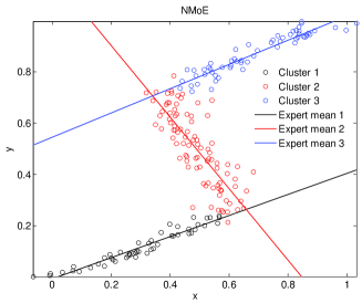
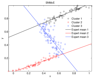
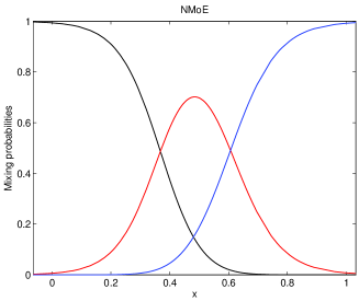
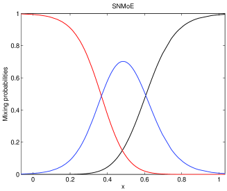
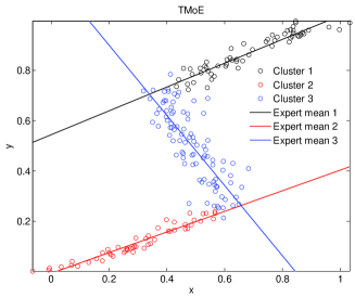
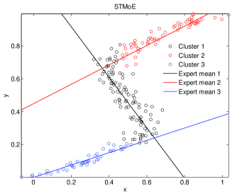
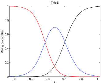
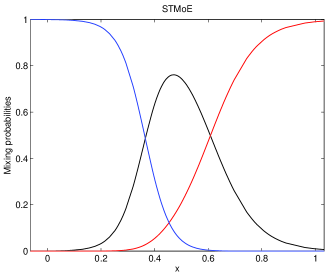
Figure 1: Fitting the NMoE model and the three proposed non-normal mixture of experts models (SNMoE, TNMoE, STMoE) to the toy data set analyzed in Bishop and Svensén (2003).

12.3 Experiments on simulation data sets

In this section we perform an experimental study on simulated data sets to apply and assess the proposed models. Two sets of experiments have been performed. The first experiment aims at observing the effect of the sample size on the estimation quality and the second one aims at observing the impact of the presence of outliers in the data on the estimation quality, that is the robustness of the models.

12.3.1 Experiment 1

For this first experiment on simulated data, each simulated sample consisted of $n$ observations with increasing values of the sample size $n:50,100,200,500,1000$. The simulated data are generated from a two component mixture of linear experts, that is $K=2,p=q=1$. The covariate variables $(\boldsymbol{x}_{i},\boldsymbol{r}_{i})$ are simulated such that $\boldsymbol{x}_{i}=\boldsymbol{r}_{i}=(1,x_{i})^{T}$ where $x_{i}$ is simulated uniformly over the interval $(-1,1)$. We consider each of the four models for data generation (NNMoE, SNMoE, TMoE, STMoE), that is, given the covariates, the response $y_{i}|\{\boldsymbol{x}_{i},\boldsymbol{r}_{i};\boldsymbol{\varPsi}\}$ is simulated according to the generative process of the models (3), (14), (36), and (14). For each generated sample, we fit each of the four models. Thus, the results are reported for all the models with data generated from each of the models. We consider the mean square error (MSE) between each component of the true parameter vector and the estimated one, which is given by $|\!|\boldsymbol{\varPsi}_{j}-\hat{\boldsymbol{\varPsi}}_{j}|\!|^{2}$. The squared errors are averaged on 100 trials. The used simulation parameters $\boldsymbol{\varPsi}$ for each model are given in Table 1.

	parameters
component 1	$\boldsymbol{\alpha}_{1}=(0,10)^{T}$	$\boldsymbol{\beta}_{1}=(0,1)^{T}$	$\sigma_{1}=0.1$	$\lambda_{1}=3$	$\nu_{1}=5$
component 2	$\boldsymbol{\alpha}_{2}=(0,0)^{T}$	$\boldsymbol{\beta}_{2}=(0,-1)^{T}$	$\sigma_{2}=0.1$	$\lambda_{2}=-10$	$\nu_{2}=7$

Table 1: Parameter values used in simulation.

12.3.2 Obtained results

Tables LABEL:tab._MSE_for_the_paramters:_SNMoE->SNMoE, LABEL:tab._MSE_for_the_paramters:_TMoE->TMoE, and LABEL:tab._MSE_for_the_paramters:_STMoE->STMoE show the obtained results in terms of the MSE for respectively the SNMoE, the TMoE, and the STMoE. One can observe that, for the three proposed models, the parameter estimation error is decreasing as $n$ increases, which confirms the convergence property of the maximum likelihood estimator For details on the convergence property of the MLE for mixture of experts, see for example (Jiang and Tanner, 1999). One can also observe that the error decreases significantly for $n\geq 500$, especially for the regression coefficients and the scale parameters.

In addition to the previously showed results, we plotted in Figures 2, 3, 4, and 5 the estimated quantities provided by applying the proposed models and their true counterparts for $n=500$ for the same the data set which was generated according the NMoE model. The upper-left plot of each of these figures shows the estimated mean function, the estimated expert component mean functions, and the corresponding true ones. The upper-right plot shows the estimated mean function and the estimated confidence region computed as plus and minus twice the estimated (pointwise) standard deviation of the model as presented in Section 9, and their true counterparts. The middle-left plot shows the true expert component mean functions and the true partition, and the middle-right plot shows their estimated counterparts. Finally, the bottom-left plot shows the log-likelihood profile during the EM iterations and the bottom-right plot shows the estimated mixing probabilities.

One can clearly see that the estimations provided by each of the proposed models are very close to the true ones which correspond to those of the NMoE model in this case. This provides an additional support to the fact that the proposed algorithms perform well and the corresponding proposed models are good generalizations of the normal mixture of experts (NMoE), as they clearly approach the NMoE as shown in this simulated example.

Figure 6 shows the true and estimated MoE mean functions and expert mean functions by fitting the proposed NNMoE models to a simulated data set of $n=500$ observations. Each model was considered for data generation. The upper plot corresponds to the SNMoE model, the middle plot to the TMoE model and the bottom plot to the STMoE model. Finally, Figure 7 shows the corresponding true and estimated partitions. Again, one can clearly see that both the estimated models are precise. The fitted functions are close to the true ones. In addition, one can also see that the partitions estimated by the NNMoE models are close the actual partitions. The proposed NNMoE models can therefore be used as alternative to the NMoE model for both regression and model-based clustering.

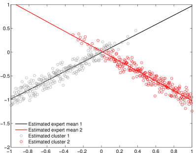
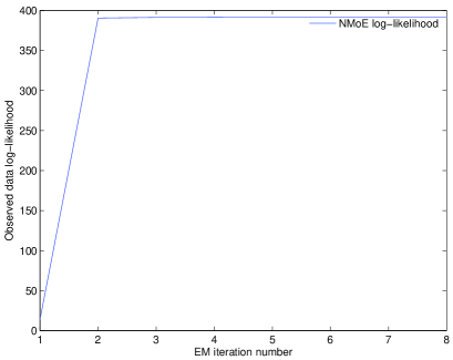
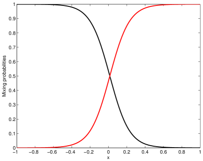
Figure 2: Fitted NMoE model to a data set generated according to the NMoE model.

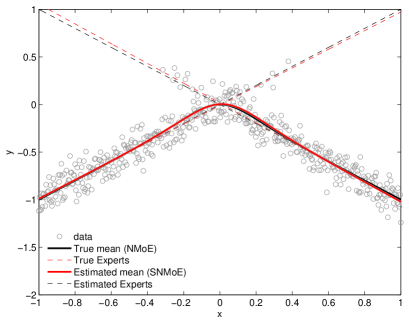
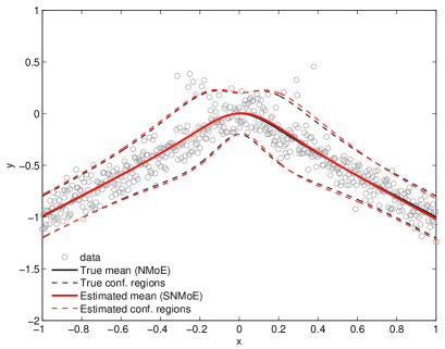
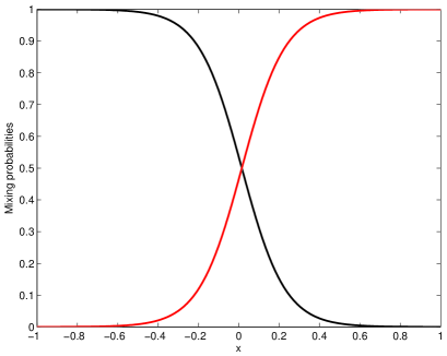
Figure 3: Fitted SNMoE model to a data set generated according to the NMoE model.

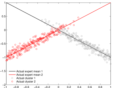
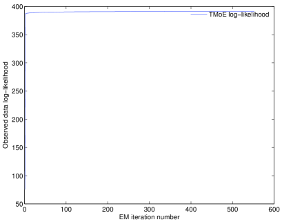
Figure 4: Fitted TMoE model to a data set generated according to the NMoE model.

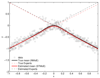
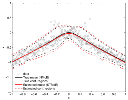
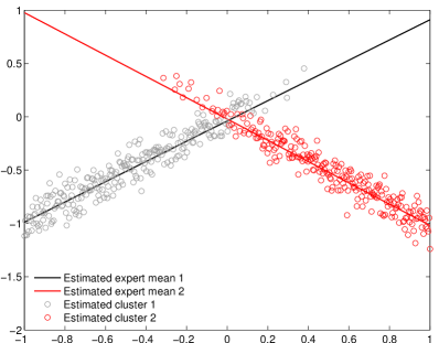
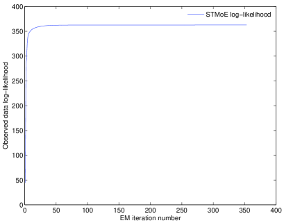
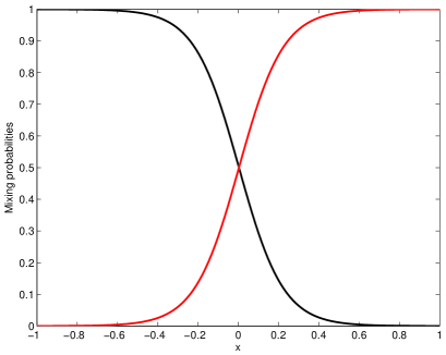
Figure 5: Fitted STMoE model to a data set generated according to the NMoE model.

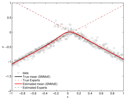
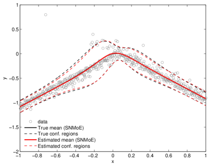
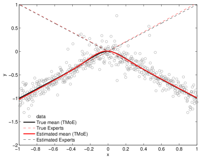
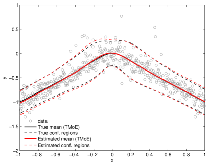
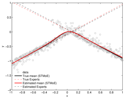
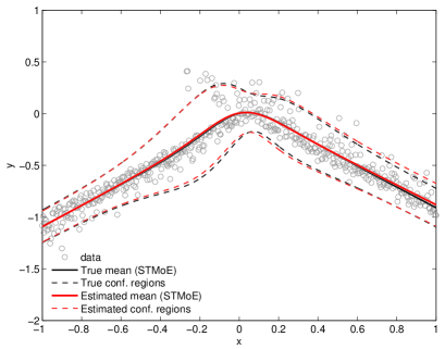
Figure 6: The true and estimated mean function and expert mean functions by fitting the proposed NNMoE models to a simulated data set of $n=500$ observations. Up: the SNMoE model; Middle: the TMoE model; Bottom: the STMoE model.

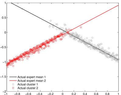
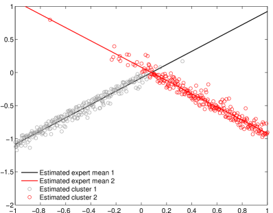
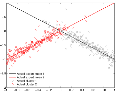
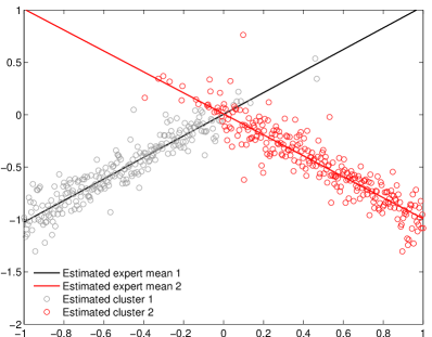
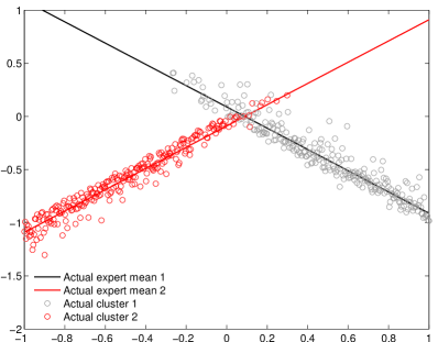
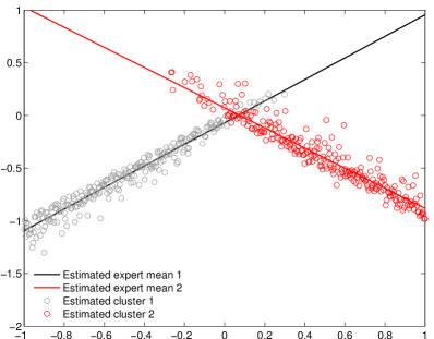
Figure 7: The true and estimated partitions by fitting the proposed NNMoE models to the simulated data set shown in Figure 6. Up: the SNMoE model; Middle: the TMoE model; Bottom: the STMoE model.

12.3.3 Experiment 2

In this experiment we examine the robustness of the proposed models to outliers versus the standard NMoE one. For that, we considered each of the four models (NMoE, SNMoE, TMoE, and STMoE) for data generation. For each generated sample, each of the four models in considered for the inference. The data were generated exactly in the same way as in Experiment 1, except for some observations which were generated with a probability $c$ from a class of outliers. We considered the same class of outliers as in Nguyen and McLachlan (2014), that is the predictor $x$ is generated uniformly over the interval $(-1,1)$ and the response $y$ is set the value $-2$. We apply the MoE models by setting the covariate vectors as before, that is, $\boldsymbol{x}=\boldsymbol{r}=(1,x)^{T}$. We considered varying probability of outliers $c=0\%,1\%,2\%,3\%,4\%,5\%$ and the sample size of the generated data is $n=500$. An example of simulated sample containing $5\%$ outliers is shown in Figure 8. As a criterion of evaluation of the impact of the outliers on the quality of the results, we considered the MSE between the true regression mean function and the estimated one. This MSE is calculated as $\frac{1}{n}\sum_{i=1}^{n}\!|\!|\!\mathbb{E}_{{\it\boldsymbol{\varPsi}}}(Y_{i}|\boldsymbol{r}_{i},\boldsymbol{x}_{i})-\mathbb{E}_{{\it\hat{\boldsymbol{\varPsi}}}}(Y_{i}|\boldsymbol{r}_{i},\boldsymbol{x}_{i})\!|\!|^{2}$ where the expectations are computed as in Section 9.

12.3.4 Obtained results

Table LABEL:tab._MSE_for_the_mean_function_-_Noisy_simulated_data_:_All->all shows, for each of the fours models, the results in terms of mean squared error between the true mean function and the estimated one, for an increasing number of outliers in the data. First, one can see that, when there is no outliers ($c=0\%$), the error of the TMoE is less than those of the other models, for the four situations, that is including the case where the data are not generated according to the TMoE model, which is somewhat surprising. This includes the case where the data aregenrated according to the NMoE model, for which the TMoE error is slightly less than the one of the NMoE model. Then, it can be seen that when there is outliers, the TMoE model outperforms the other models for almost all the situations, except the one in which the data are generated according to the STMoE model. When the data do not contain outliers and are generated from the STMoE, this one indeed outperforms the NMoE and SNMoE models. For the situation when there is no outliers and the data are generated according to the TMoE or the STMoE, these two models may provide quasi-identical results. In the case of presence of outliers in data generated from the STMoE, this one outperforms the NMoE and SNMoE models for all the situations, and outperforms the TMoE for the majority of situations, namely when the number of the outliers is more than $2\%$. One can also see that, for all the situations with outliers, as expected, the TMoE and STMoE models always provide the best results. These two models are indeed much more robust to outliers compared to the normal and skew-normal ones because the expert components in these two models follow a robust distribution, that is the $t$ distribution for the TMoE, and the skew $t$ distribution for the STMoE. The NMoE and SNMoE are sensitive to outliers. When there is outliers, the SNMoE behavior is comparable to the one of the NMoE. However, when the number of outliers is increasing, it can be seen that the increase in the error of the NMoE and SNMoE model is more pronounced compared to the one of the TMoE and STMoE models. The error for both the TMoE and STMoE may indeed slightly increase, remain stable or even decrease in some situations. This supports the expected robustness of the TMoE and STMoE models.

To highlight the robustness to noise of the TMoE and STMoE models, in addition to the previously shown numerical results, figures 8, 9, 10, and 11 show an example of results obtained on the same data set by, respectively, the NMoE, the SNMoE, TMoE, and the STMoE. The data are generated by the NMoE model and contain $c=5\%$ of outliers.

In this example, we clearly see that both the NMoE model and the SNMoE are severely affected by the outliers. They provide a rough fit especially for the second component whose estimation is affected by the outliers. However, one can see that both the TMoE and the STMoE model clearly provide a precise fit; the estimated mean functions and expert components are very close to the true ones. The TMoE and the STMoE are robust to outliers, in terms of estimating the true model as well as in terms of estimating the true partition of the data (as shown in the middle plots of the data). Notice that for the TMoE and the STMoE, the confidence regions are not shown because for this situation the estimated degrees of freedom are less than $2$ ($1.5985$ and $1.5253$ for the TMoE, and $1.6097$ $1.5311$ for the STMoE); Hence the variance for these models in that case is not defined (see Section 9). The TMoE and STMoE models provide indeed components with small degrees of freedom corresponding to highly heavy tails, which allow to handle outliers in this noisy case.

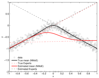
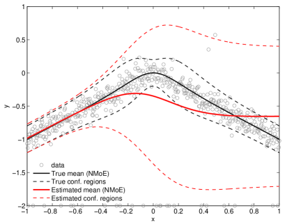
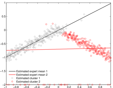
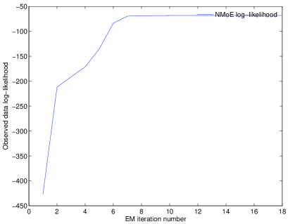
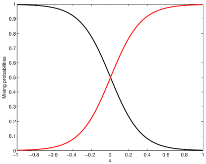
Figure 8: Fitted NMoE model to a data set of $n=500$ observations generated according to the NMoE model and including $5\%$ of outliers.

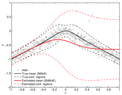
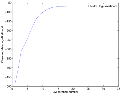
Figure 9: Fitted SNMoE model to a data set of $n=500$ observations generated according to the NMoE model and including $5\%$ of outliers.

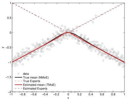
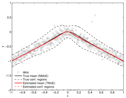
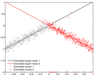
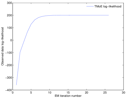
Figure 10: Fitted TMoE model to a data set of $n=500$ observations generated according to the NMoE model and including $5\%$ of outliers.

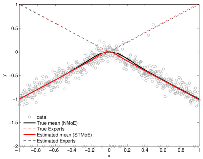
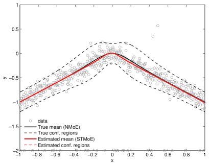
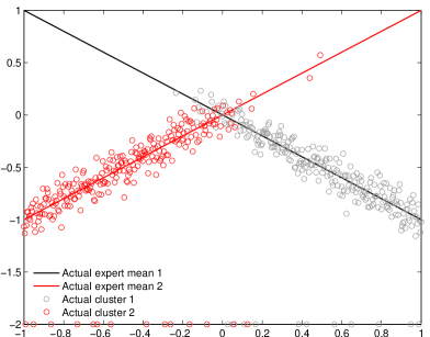
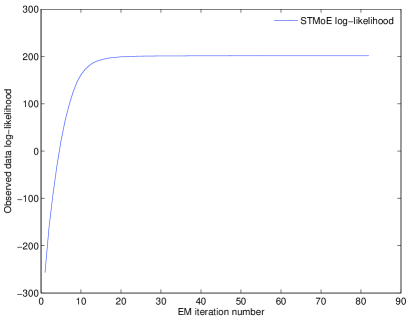
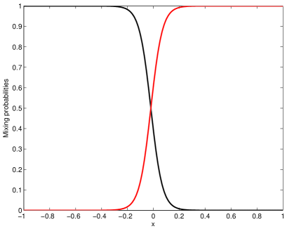
Figure 11: Fitted STMoE model to a data set of $n=500$ observations generated according to the NMoE model and including $5\%$ of outliers.

12.4 Application to two real-world data sets

In this section, we consider an application to two real-world data sets: the tone perception data set and the temperature anomalies data set shown in Figure 12.

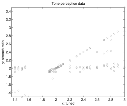
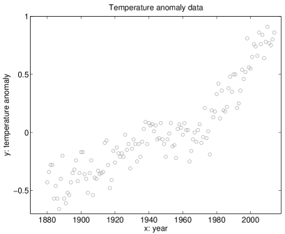
Figure 12: Scatter plots of the tone perception data and the temperature anomalies data.

12.4.1 Tone perception data set

The first analyzed data set is the real tone perception data set which goes back to Cohen (1984). It was recently studied by Bai et al. (2012) and Song et al. (2014) by using robust regression mixture models based on, respectively, the $t$ distribution and the Laplace distribution. In the tone perception experiment, a pure fundamental tone was played to a trained musician. Electronically generated overtones were added, determined by a stretching ratio (“stretch ratio” = 2) which corresponds to the harmonic pattern usually heard in traditional definite pitched instruments. The musician was asked to tune an adjustable tone to the octave above the fundamental tone and a “tuned” measurement gives the ratio of the adjusted tone to the fundamental. The obtained data consists of $n=150$ pairs of “tuned” variables, considered here as predictors ($x$), and their corresponding “strech ratio” variables considered as responses ($y$). To apply the proposed MoE models, we set the response $y_{i}(i=1,\ldots,150)$ as the “strech ratio” variables and the covariates $\boldsymbol{x}_{i}=\boldsymbol{r}_{i}=(1,x_{i})^{T}$ where $x_{i}$ is the “tuned” variable of the $i$th observation. We also follow the study in Bai et al. (2012) and Song et al. (2014) by using two mixture components. Model selection results are given later in Table LABEL:tab._Model_selection_Tone_data.

Figure 13 shows the scatter plots of the tone perception data and the linear expert components of the fitted NMoE model and the proposed SNMoE, TMoE, and STMoE models. One can observe that we obtain a good fit with all the models. The NMoE and SNMoE are quasi-identical, and differ very slightly from those of the TMoE and STMoE, which are very similar. The two regression lines may correspond to correct tuning and tuning to the first overtone, respectively, as analyzed in Bai et al. (2012).

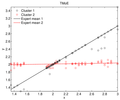
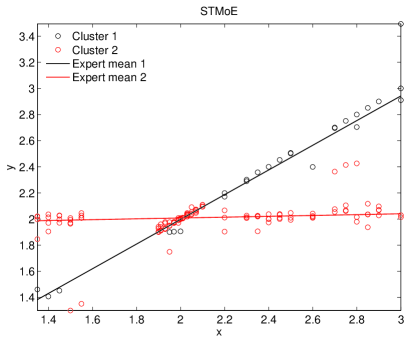
Figure 13: The fitted MoLE to the original tone data set. Upper-left: NMoE model, Upper-right: SNMoE model, Bottom-left: TMoE model, Bottom-right: STMoE model. The predictor $x$ is the actual tone ratio and the response $y$ is the perceived tone ratio.

Figure 14 shows the log-likelihood profiles for each of the four models. It can namely be seen that training the $t$ mixture of experts for this experiment may take more iterations than the normal and the skew-normal MoE models. The STMoE has indeed more parameters to estimate than the other ones. However, in terms of computing time, all the models converge in only few seconds on a personal laptop (withe 2,9 GHz processor and and 8 GB memory).

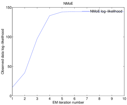
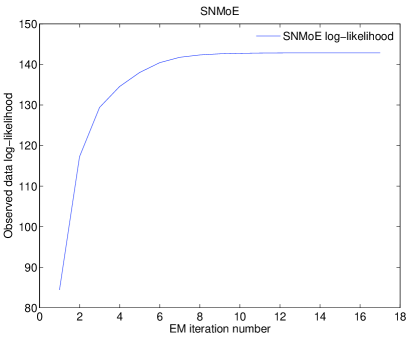
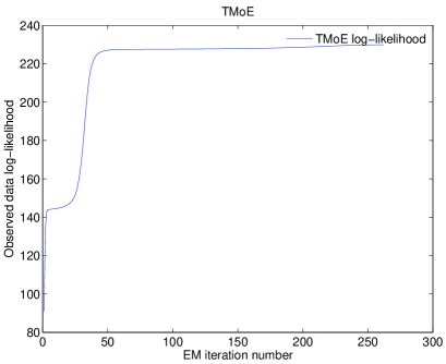
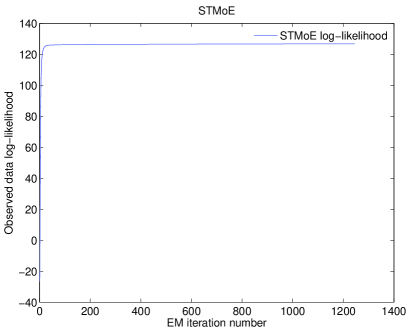
Figure 14: The log-likelihood during the EM iterations when fitting the MoLE models to the original tone data set. Upper-left: NMoE model, Upper-right: SNMoE model, Bottom-left: TMoE model, Bottom-right: STMoE model.

The values of estimated parameters for the tone perception data set are given in Table LABEL:tab._Estimated_parameters_for_the_tone_perception_data_set. One can see that the regression coefficients are very similar for all the models, except for the first component of the TMoE model. This can be observed on the fit in Figure 13 where the first expert component for the TMoE model slightly differ from the one of the other ones. One can also see that the SNMoE model parameters are identical to those of the NMoE, with a skewness close to zero. For the STMoE model, it retrieves a skewed component and with high degrees of freedom compared to the other component. This component may be seen as approaching the one of the SNMoE model, while the second one in approaching a $t$ distribution, that is the one of the TMoE model.

We also performed a model selection procedure on this data set to choose the best number of MoE components for a number of components between 1 and 5. We used BIC, AIC, and ICL. Table LABEL:tab._Model_selection_Tone_data gives the obtained values of the model selection criteria. One can see that for the NMoE model overestimate the number oc components. AIC performs poorly for all the models. BIC provides the correct number of components for the three proposed models. ICL too estimated the correct number of components for both the SNMoE and STMoE models, but hesitates between 2 (the correct number) and 3 components for the TMoE model. One can conclude that the BIC is the criterion to be suggested for the analysis.

Now we examine the sensitivity of the MoE models to outliers based on this real data set. For this, we adopt the same scenario used in Bai et al. (2012) and Song et al. (2014) (the last and more difficult scenario) by adding 10 identical pairs $(0,4)$ to the original data set as outliers in the $y$-direction, considered as high leverage outliers. We apply the MoE models in the same way as before.

The upper plots in Figure 15 show that the normal and the skew-normal mixture of experts provide almost identical fits and are sensitives to outliers. However, in both cases, compared to the normal regression mixture result in Bai et al. (2012), and the Laplace regression mixture and the $t$ regression mixture results in Song et al. (2014), the fitted NMoE and SNMoE model are affected less severely by the outliers This may be attributed to the fact that the mixing proportions here are depending on the predictors, which is not the case in these regression mixture models, namely the ones of Bai et al. (2012), and Song et al. (2014). One can also see that, even the regression mean functions are affected severely by the outliers, the provided partitions are still reasonable and similar to those provided in the previous non-noisy case. Then, the bottom plots in Figure 15 clearly show that the TMoE and the STMoE provide a robust good fit. For the TMoE, the obtained fit is quasi-identical to the first one on the original data without outliers, shown in the bottom-left plot of Figure 13. For the STMoE, even if the results differ very slightly compared to the case with outliers, the obtained fits for both situations (with and without outliers) are very reasonable. Moreover, we notice that, as showed in Song et al. (2014), for this situation with outliers, the $t$ mixture of regressions fails; The fit is affected severely by the outliers. However, for the proposed TMoE and STMoE, the ten high leverage outliers have no significant impact on the fitted experts. This is because here the mixing proportions depend on the inputs, which is not the case for the regression mixture model described in Song et al. (2014).

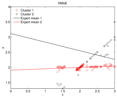
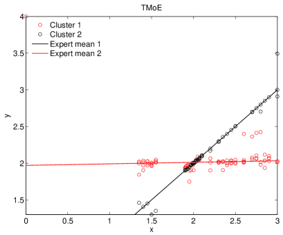
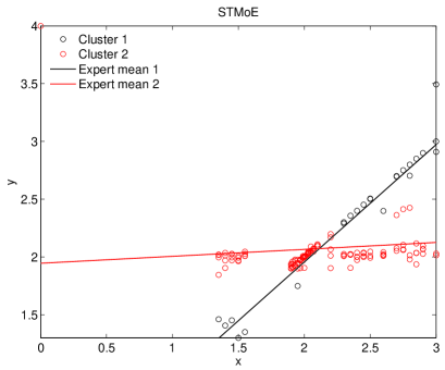
Figure 15: Fitting MoLE to the tone data set with ten added outliers $(0,4)$. Upper-left: NMoE model, Upper-right: SNMoE model, Bottom-left: TMoE model, Bottom-right: STMoE model. The predictor $x$ is the actual tone ratio and the response $y$ is the perceived tone ratio.

Figure 16 shows the log-likelihood profiles for each of the four models, which show a similar behavior than the one in the case without outliers.

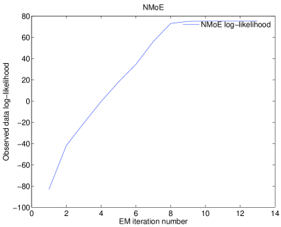
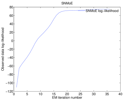
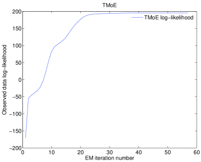
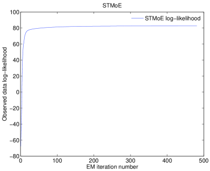
Figure 16: The log-likelihood during the EM iterations when fitting the MoLE models to the tone data set with ten added outliers $(0,4)$. Upper-left: NMoE model, Upper-right: SNMoE model, Bottom-left: TMoE model, Bottom-right: STMoE model.

The values of estimated MoE parameters in this case with outliers are given in Table LABEL:tab._Estimated_parameters_for_the_tone_perception_data_set_with_outliers. One can see that the SNMoE model parameters are identical to those of the NMoE, with a skewness close to zero. The regression coefficients for the second expert component are very similar for all the models. For the first component, the TMoE model is still retrieving a more heavy tailed component. For the STMoE model, it retrieves a skewed normal component while the second component in approaching a $t$ distribution with a small degrees of freedom.

12.4.2 Temperature anomalies data set

In this experiment, we examine another real-world data set related to climate change analysis. The NASA GISS Surface Temperature (GISTEMP) analysis provides a measure of the changing global surface temperature with monthly resolution for the period since 1880, when a reasonably global distribution of meteorological stations was established. The GISS analysis is updated monthly, however the data presented here are updated annually as issued from the Carbon Dioxide Information Analysis Center (CDIAC), which has served as the primary climate-change data and information analysis center of the U.S. Department of Energy since 1982. The data consist of $n=135$ yearly measurements of the global annual temperature anomalies (in degrees C) computed using data from land meteorological stations for the period of $1882-2012$. These data have been analyzed earlier by Hansen et al. (1999, 2001) and recently by Nguyen and McLachlan (2014) by using the Laplace mixture of linear experts (LMoLE).

To apply the proposed non-normal mixture of expert models, we consider mixtures of two experts as in Nguyen and McLachlan (2014). This number of components is also the one provided by the model selection criteria as shown later in Table LABEL:tab._Model_selection_temprature_anomalies_data. Indeed, as mentioned by Nguyen and McLachlan (2014), Hansen et al. (2001) found that the data could be segmented into two periods of global warming (before 1940 and after 1965), separated by a transition period where there was a slight global cooling (i.e. 1940 to 1965). Documentation of the basic analysis method is provided by Hansen et al. (1999, 2001). We set the response $y_{i}(i=1,\ldots,135)$ as the temperature anomalies and the covariates $\boldsymbol{x}_{i}=\boldsymbol{r}_{i}=(1,x_{i})^{T}$ where $x_{i}$ is the year of the $i$th observation.

Figures 17, 18, and 19 respectively show, for each of the MoE models, the two fitted linear expert components, the corresponding means and confidence regions computed as plus and minus twice the estimated (pointwise) standard deviation as presented in Section 9, and the log-likelihood profiles. One can observe that the four models are successfully applied on the data set and provide very similar results. These results are also similar to those found by Nguyen and McLachlan (2014) who used a Laplace mixture of linear experts.

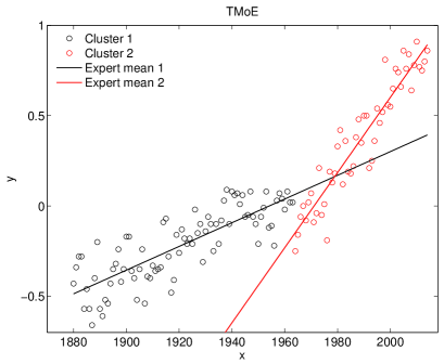
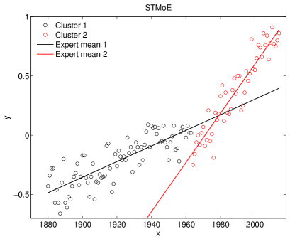
Figure 17: Fitting the MoLE models to the temperature anomalies data set. Upper-left: NMoE model, Upper-right: SNMoE model, Bottom-left: TMoE model, Bottom-right: STMoE model. The predictor $x$ is the year and the response $y$ is the temperature anomaly.

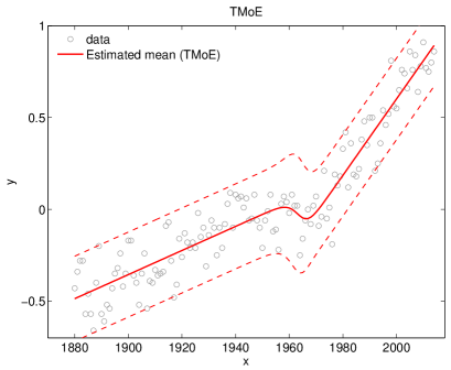
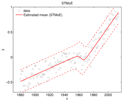
Figure 18: The fitted MoLE models to the temperature anomalies data set. Upper-left: NMoE model, Upper-right: SNMoE model, Bottom-left: TMoE model, Bottom-right: STMoE model. The predictor $x$ is the year and the response $y$ is the temperature anomaly. The shaded region represents plus and minus twice the estimated (pointwise) standard deviation as presented in Section 9.

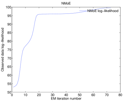
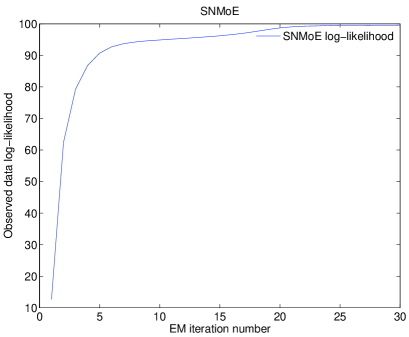
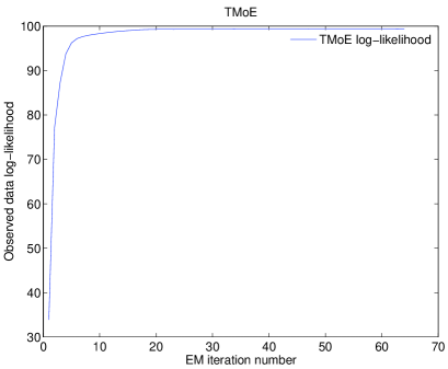
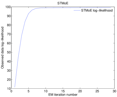
Figure 19: The log-likelihood during the EM iterations when fitting the MoLE models to the temperature anomalies data set. Upper-left: NMoE model, Upper-right: SNMoE model, Bottom-left: TMoE model, Bottom-right: STMoE model.

The values of estimated MoE parameters for the temperature anomalies data set are given in Table LABEL:tab._estimated_parameters_for_the_temperature_anomalies_data_set. One can see that the parameters common for the all models are quasi-identical. It can also be seen that the SNMoE model provides s a fit with a skewness very close to zero. Similarly, the STMoE model provide a solution with a skewness close to zero. This may support the hypothesis of non-asymmetry for this data set. Then, both the TMoE and STMoE fits provide a degrees of freedom more than 17, which tends to approach a normal distribution. On the other hand, the regression coefficients are also similar to those found by Nguyen and McLachlan (2014) who used a Laplace mixture of linear experts.

We performed a model selection procedure on the temperature anomalies data set to choose the best number of MoE components from values between 1 and 5. Table LABEL:tab._Model_selection_temprature_anomalies_data gives the obtained values of the used model selection criteria, that is BIC, AIC, and ICL. One can see that, except the result provided by AIC for the NMoE model which provide a high number of components, all the others results provide evidence for two components in the data.

13 Conclusion and future work

In this paper, we proposed new non-normal MoE models, which generalize the normal MoE. They are based on the skew-normal, $t$ and skew $t$ distribution and are respectively the SNMoE, TMoE, and STMoE. The SNMoE model is suggested for non-symmetric data, the TMoE for data with possibly outliers and heavy tail, and the STMoE is suggested for both possibly non-symmetric, heavy tailed and noisy data. We developed EM-type algorithms to infer each of the proposed models and described the use of the models in non-linear regression and prediction as well as in model-based clustering. The developed models are successfully applied on simulated and real data sets. The results obtained on simulated data confirm the good performance of the models in terms of density estimation, non-linear regression function approximation and clustering. In addition, the simulation results provide evidence of the robustness of the TMoE and STMoE models to outliers, compared to the normal alternative models. The proposed models were also successfully applied to two different real data sets, including a situation with outliers. The model selection using information criteria tends to promote using BIC against in particular AIC which may perform poorly in the analyzed data. The obtained results support the potential benefit of the proposed approaches for practical applications.

In this paper, we only considered the MoE in their standard (non-hierarchical) version. One interesting future direction is therefore to extend the proposed models to the hierarchical mixture of experts framework (Jordan and Jacobs, 1994). Furthermore, a natural future extension of this work is to consider the case of MoE for multiple regression on multivariate data rather than simple regression on univariate data.

References

- Akaike (1974) H. Akaike. A new look at the statistical model identification. IEEE Transactions on Automatic Control, 19(6):716–723, 1974.
- Azzalini (1985) A. Azzalini. A class of distributions which includes the normal ones. Scandinavian Journal of Statistics, pages 171–178, 1985.
- Azzalini (1986) A. Azzalini. Further results on a class of distributions which includes the normal ones. Scandinavian Journal of Statistics, pages 199–208, 1986.
- Azzalini and Capitanio (2003) A. Azzalini and A. Capitanio. Distributions generated by perturbation of symmetry with emphasis on a multivariate skew t distribution. Journal of the Royal Statistical Society, Series B, 65:367–389, 2003.
- Bai et al. (2012) Xiuqin Bai, Weixin Yao, and John E. Boyer. Robust fitting of mixture regression models. Computational Statistics & Data Analysis, 56(7):2347 – 2359, 2012.
- Biernacki et al. (2000) C. Biernacki, G. Celeux, and G Govaert. Assessing a mixture model for clustering with the integrated completed likelihood. IEEE Transactions on Pattern Analysis and Machine Intelligence, 22(7):719–725, 2000.
- Bishop and Svensén (2003) C. Bishop and M. Svensén. Bayesian hierarchical mixtures of experts. In In Uncertainty in Artificial Intelligence, 2003.
- Brent (1973) Richard P. Brent. Algorithms for minimization without derivatives. Prentice-Hall series in automatic computation. Englewood Cliffs, N.J. Prentice-Hall, 1973. ISBN 0-13-022335-2.
- Chamroukhi (2010) F. Chamroukhi. Hidden process regression for curve modeling, classification and tracking. Ph.D. thesis, Université de Technologie de Compiègne, Compiègne, France, 2010.
- Chamroukhi et al. (2009a) F. Chamroukhi, A. Samé, G. Govaert, and P. Aknin. A regression model with a hidden logistic process for feature extraction from time series. In International Joint Conference on Neural Networks (IJCNN), 2009a.
- Chamroukhi et al. (2009b) F. Chamroukhi, A. Samé, G. Govaert, and P. Aknin. Time series modeling by a regression approach based on a latent process. Neural Networks, 22(5-6):593–602, 2009b.
- Chamroukhi et al. (2010) F. Chamroukhi, A. Samé, G. Govaert, and P. Aknin. A hidden process regression model for functional data description. application to curve discrimination. Neurocomputing, 73(7-9):1210–1221, March 2010.
- Chen et al. (1999) K. Chen, L. Xu, and H. Chi. Improved learning algorithms for mixture of experts in multiclass classification. Neural Networks, 12(9):1229–1252, 1999.
- Cohen (1984) Elizabeth A. Cohen. Some effects of inharmonic partials on interval perception. Music Perception, 1, 1984.
- Dempster et al. (1977) A. P. Dempster, N. M. Laird, and D. B. Rubin. Maximum likelihood from incomplete data via the EM algorithm. Journal of The Royal Statistical Society, B, 39(1):1–38, 1977.
- Frühwirth-Schnatter (2006) S. Frühwirth-Schnatter. Finite Mixture and Markov Switching Models (Springer Series in Statistics). Springer Verlag, New York, 2006.
- Frühwirth-Schnatter and Pyne (2010) S. Frühwirth-Schnatter and S. Pyne. Bayesian inference for finite mixtures of univariate and multivariate skew-normal and skew-t distributions. Biostatistics, 11(2):317–336, 2010.
- Genton et al. (2001) Marc G. Genton, Li He, and Xiangwei Liu. Moments of skew-normal random vectors and their quadratic forms. Statistics & Probability Letters, 51:319–325, 2001.
- Green (1984) P. Green. Iteratively reweighted least squares for maximum likelihood estimation, and some robust and resistant alternatives. Journal of The Royal Statistical Society, B, 46(2):149–192, 1984.
- Hansen et al. (1999) J. Hansen, R. Ruedy, J. Glascoe, and M. Sato. Giss analysis of surface temperature change. Journal of Geophysical Research, 104:30997–31022, 1999.
- Hansen et al. (2001) J. Hansen, R. Ruedy, Sato M., M. Imhoff, W. Lawrence, D. Easterling, T. Peterson, and T. Karl. A closer look at united states and global surface temperature change. Journal of Geophysical Research, 106:23947–23963, 2001.
- Henze (1986) Norbert Henze. A probabilistic representation of the skew-normal distribution. Scandinavian Journal of Statistics, pages 271–275, 1986.
- Huang et al. (2015) Chao Huang, Martin Styner, and Hongtu Zhu. Clustering high-dimensional landmark-based two-dimensional shape data. Journal of the American Statistical Association, April 2015. doi: http://dx.doi.org/10.1080/01621459.2015.1034802.
- J. Q. Shi and Titterington (2005) Roderick Murray-Smith J. Q. Shi and D. M. Titterington. Hierarchical gaussian process mixtures for regression. Statistics and Computing, 15(1):31–41, 2005.
- Jacobs et al. (1991) R. A. Jacobs, M. I. Jordan, S. J. Nowlan, and G. E. Hinton. Adaptive mixtures of local experts. Neural Computation, 3(1):79–87, 1991.
- Jiang and Tanner (1999) Wenxin Jiang and M. A. Tanner. On the asymptotic normality of hierarchical mixtures-of-experts for generalized linear models. IEEE Transactions on Information Theory, 46:1005–1013, 1999.
- Jordan and Jacobs (1994) M. I. Jordan and R. A. Jacobs. Hierarchical mixtures of experts and the EM algorithm. Neural Computation, 6:181–214, 1994.
- Jordan and Xu (1995) M. I. Jordan and L. Xu. Convergence results for the EM approach to mixtures of experts architectures. Neural Networks, 8(9):1409–1431, 1995.
- Kent et al. (1994) J.T. Kent, D.E. Tyler, and Y Vardi. A curious likelihood identity for the multivariate t-distribution. Communications in Statistics - Simulation and Computation, 23:441–453, 1994.
- Lee and McLachlan (2013a) Sharon X. Lee and Geoffrey J. McLachlan. On mixtures of skew normal and skew t-distributions. Advances in Data Analysis and Classification, 7(3):241–266, 2013a.
- Lee and McLachlan (2013b) Sharon X. Lee and Geoffrey J. McLachlan. Model-based clustering and classification with non-normal mixture distributions. Statistical Methods and Applications, 22(4):427–454, 2013b.
- Lee and McLachlan (2014) Sharon X. Lee and Geoffrey J. McLachlan. Finite mixtures of multivariate skew t-distributions: some recent and new results. Statistics and Computing, 24(2):181–202, 2014.
- Lee and McLachlan (2015) Sharon X. Lee and Geoffrey J. McLachlan. Finite mixtures of canonical fundamental skew t-distributions. Statistics and Computing (To appear), 2015. doi: 10.1007/s11222-015-9545-x.
- Lin (2010) Tsung I. Lin. Robust mixture modeling using multivariate skew t distributions. Statistics and Computing, 20(3):343–356, 2010.
- Lin et al. (2007a) Tsung I. Lin, Jack C. Lee, and Wan J. Hsieh. Robust mixture modeling using the skew t distribution. Statistics and Computing, 17(2):81–92, 2007a.
- Lin et al. (2007b) Tsung I. Lin, Jack C. Lee, and Shu Y Yen. Finite mixture modelling using the skew normal distribution. Statistica Sinica, 17:909–927, 2007b.
- Liu and Rubin (1995) Chuanhai Liu and Donald B. Rubin. ML estimation of the t distribution using EM and its extensions, ECM and ECME. Statistica Sinica, 5:19–39, 1995.
- McLachlan and Krishnan (2008) G. J. McLachlan and T. Krishnan. The EM algorithm and extensions. New York: Wiley, second edition, 2008.
- McLachlan and Peel. (2000) G. J. McLachlan and D. Peel. Finite mixture models. New York: Wiley, 2000.
- Mclachlan and Peel (1998) Geoffrey J. Mclachlan and David Peel. Robust cluster analysis via mixtures of multivariate t-distributions. In Lecture Notes in Computer Science, pages 658–666. Springer-Verlag, 1998.
- Meng and Rubin (1993) X. L. Meng and D. B. Rubin. Maximum likelihood estimation via the ECM algorithm: A general framework. Biometrika, 80(2):267–278, 1993.
- Ng and McLachlan (2004) Shu-Kay Ng and Geoffrey J. McLachlan. Using the em algorithm to train neural networks: misconceptions and a new algorithm for multiclass classification. IEEE Transactions on Neural Networks, 15(3):738–749, 2004.
- Nguyen and McLachlan (2014) Hien D. Nguyen and Geoffrey J. McLachlan. Laplace mixture of linear experts. Computational Statistics & Data Analysis, (0):–, 2014. ISSN 0167-9473. doi: http://dx.doi.org/10.1016/j.csda.2014.10.016.
- Peel and Mclachlan (2000) D. Peel and G. J. Mclachlan. Robust mixture modelling using the t distribution. Statistics and Computing, 10:339–348, 2000.
- Pyne et al. (2009) S Pyne, X Hu, K Wang, E Rossin, TI Lin, LM Maier, C Baecher-Allan, GJ McLachlan, P Tamayo, DA Hafler, PL De Jager, and JP Mesirow. Automated high-dimensional flow cytometric data analysis. Proceedings of the National Academy of Sciences USA, 2009. doi: 106:8519?8524.
- Rasmussen and Ghahramani (2001) Carl Edward Rasmussen and Zoubin Ghahramani. Infinite mixtures of gaussian process experts. In In Advances in Neural Information Processing Systems 14, pages 881–888. MIT Press, 2001.
- (47) R. Ruedy, M. Sato, and K. Lo. NASA GISS surface temperature (GISTEMP) analysis. DOI: 10.3334/CDIAC/cli.001. Center for Climate Systems Research, NASA Goddard Institute for Space Studies 2880 Broadway, New York, NY 10025 USA.
- Schwarz (1978) G. Schwarz. Estimating the dimension of a model. Annals of Statistics, 6:461–464, 1978.
- Shi and Choi (2011) J. Q. Shi and T. Choi. Gaussian Process Regression Analysis for Functional Data. Chapman & Hall/CRC Press, 2011.
- Song et al. (2014) Weixing Song, Weixin Yao, and Yanru Xing. Robust mixture regression model fitting by laplace distribution. Computational Statistics & Data Analysis, 71(0):128 – 137, 2014.
- Waterhouse (1997) S. R. Waterhouse. Classification and regression using Mixtures of Experts. PhD thesis, Department of Engineering, Cambridge University, 1997.
- Waterhouse et al. (1996) Steve Waterhouse, David Mackay, and Tony Robinson. Bayesian methods for mixtures of experts. In In, pages 351–357. MIT Press, 1996.
- Wei (2012) Y. Wei. Robust mixture regression models using t-distribution. Technical report, Master Report, Department of Statistics, Kansas State University, 2012.
- Yuksel et al. (2012) Seniha Esen Yuksel, Joseph N. Wilson, and Paul D. Gader. Twenty years of mixture of experts. IEEE Trans. Neural Netw. Learning Syst., 23(8):1177–1193, 2012.
- Zeller et al. (2015) C. B. Zeller, V. H. Lachos, and C.R. Cabral. Robust mixture regression modelling based on scale mixtures of skew-normal distributions. Test (revision invited), 2015.