The Condensate from Torus Knots

A. Gorsky^2,3, A. Milekhin^1,2,3,4 and N. Sopenko^1,2 

¹Institute of Theoretical and Experimental Physics, B.Cheryomushkinskaya 25, Moscow 117218, Russia

²Moscow Institute of Physics and Technology, Dolgoprudny 141700, Russia

³ Institute for Information Transmission Problems of Russian Academy of Science, B. Karetnyi 19, Moscow 127051, Russia

⁴ Department of Physics, Princeton University, Princeton, NJ 08544

gorsky@itep.ru, milekhin@itep.ru, niksopenko@gmail.com

Abstract

We discuss recently formulated instanton-torus knot duality in $\Omega$-deformed 5D SQED on $\mathbb{R}^{4}\times S^{1}$ focusing at the microscopic aspects of the condensate formation in the instanton ensemble. Using the chain of dualities and geometric transitions we embed the SQED with a surface defect into the $SU(2)$ SQCD with $N_{f}=4$ and identify the numbers $(n,m)$ of the torus $T_{n,m}$ knot as instanton charge and electric charge. The HOMFLY torus knot invariants in the fundamental representation provide entropic factor in the condensate of the massless flavor counting the degeneracy of the instanton–W-boson web with instanton and electric numbers $(n,m)$ but different spin and flavor content. Using the inverse geometrical transition we explain how our approach is related to the evaluation of the HOMFLY invariants in terms of Wilson loop in 3d CS theory. The reduction to 4D theory is briefly considered and some analogy with baryon vertex is conjectured.

1 Introduction

The clarification of the microscopic mechanism behind the formation of the condensates is the challenging problem in a quantum field theory. Usually this question is substituted by a kind of a mean field analysis. However in some cases it is possible to recognize that particular non-perturbative configuration or ensembles of the non-perturbative configurations are responsible for the condensate formation. The familiar example is evaluation of the gluino condensate in the SYM theory in terms of the gluino zero modes in the instanton background [1]. The issue is quite subtle since for instance in SU(2) SYM theory the instanton configuration saturates only the topological correlator and additional clusterization argument has to be applied to extract the condensate itself. The way out was to consider SQCD,evaluate the exact superpotential and then derive the gluino condensate using the Konishi anomaly. One more approach concerns the compactification of one coordinate, find the BPS configurations with two gluino zero modes and saturate the condensate by zero modes on these configurations [2]. The different ways of evaluation of the gluino condensate differ by the numerical factor which certainly shows that this issue is not understood properly.

The explicit Nekrasov-like evaluation of the instanton sums in the different dimensions [3] allows to attack the issue of the microscopic mechanism for condensate formation in SUSY YM theory with the new tool. The low energy effective action depends on the masses of the matter fields as parameters hence the instanton contribution to condensates can be extracted upon differentiation. On the other hand using the exact results concerning equivariant K-theory of Hilbert scheme of centered points in $\mathbb{C}^{2}$ [4] it was found that the torus knot superpolynomials can be represented along this way [5, 6]. Since K-theory of Hilbert scheme of points in $\mathbb{C}^{2}$ is intimately related to the instantons in 5D SYM theory it is natural to assume that torus knot homologies and invariants are relevant for some physical observable in $\Omega$-deformed 5d gauge theory. In [7] the instanton-torus knot duality was formulated in 5d SQCD based on the observation made in [8]. It turned out that refined torus knot invariants are involved into the formation of the massless flavor condensate.

The essentially new findings in [7] are as follows

• It was shown that the $T_{n,nk+1}$ torus knot superpolynomials are encoded in the UV properties of the condensate of the massless flavor in the 5d SYM theory with one compact dimension and 5d CS term at level k. It was the first explicit example of the evaluation of the refined knot invariant in the dual ” magnetic” approach in the instanton ensemble in the gauge theory.

• In the previous studies the invariants of the particular knots are involved into evaluation of the Wilson loops or partition functions and no any summation over the knot types was needed. In our case due to the instanton-torus knot duality the summation over instantons implies the summation over all types of the torus knots.

• In [7] we travelled across the bridge between the theories with Landau pole at $N_{f}=3$ and the asymptotically free theory at $N_{f}=1$ using the decoupling of heavy degrees of freedom. The heavy flavor in the theory with Landau pole can be substituted by the particular observable which on the other hand can be interpreted as the brane-antibrane pair.

In this paper we shall clarify the origin of the instanton-torus knot duality and the role of the torus knots invariants in the condensate formation. We shall argue that the invariants of the torus knots provide the entropic factor counting the degeneracies of the particular BPS states. Remind that the pattern for the evaluation of the knot invariants as counting of BPS states has been suggested in [9]. The useful tool to recognize the knot invariants in the topological string framework is the geometric transition [10] which occurs when the set of N topological branes wrapped the submanifold in 3 CY M in $T^{*}M$ gets substituted for $M=S^{3}$ by the resolved conifold with the complex Kahler parameter equals to $Ng_{s}$ where $g_{s}$ is the string coupling. To obtain the knot it is necessary [9] to add the Lagrangian brane $L_{K}$ with the geometry of $S^{1}\times R^{2}$ intersecting the $S^{3}$ along the knot K. Upon the geometric transition the Lagrangian brane remains hence we get the open A-model setup with $L_{K}$. It was argued that the HOMFLY polynomials count the BPS particles represented by M2 branes ending on $L_{K}$.More recently the different aspects of the representation of the torus knots in the topological string framework have been discussed in [11, 12, 13].

Our picture is somewhat close to this approach. We shall demonstrate that HOMFLY polynomials of the $T_{n,m}$ torus knots in the fundamental representation count the multiplicity of states in the instanton-W-boson web with the fixed instanton and electric quantum charges $(n,m)$. We consider the 5D SQCD with the matter in fundamental and antifundamental representations and the mass of antifundamental provides the parameter $a=q^{N}$ in the HOMFLY polynomial [7]. In our approach the counting involves the enumeration of differently oriented M2 branes corresponding to $n$ instantons and $m$ W-bosons. Since the rank of the gauge group in CS representation of HOMFLY is represented by mass of the antifundamental we shall make the inverse geometric transition representing the Kahler class of the blow-up point in resolved conifold corresponding to the antifundamental matter [14, 15]. During this inverse geometric transition we substitute the $S^{2}$ by the set of topological branes on $S^{3}$ and the instanton and W-boson M2 branes yield the torus knots in $S^{3}$.

We consider the generic electric and instanton quantum numbers and to make the instanton particles more tractable embed SQED into SU(2) 5d SQCD when the instantons and W-bosons enter the central charge at the equal footing. The generic picture for arbitrary quantum numbers can be also visualized in IIB string theory in terms of the string webs [16, 17, 18] with boundaries at the 5-brane web. The instantons and W-bosons are represented by different strings obeying the particular rules of intersection while the hypers are represented by the combination of the strings and strips. We should count the number of the different webs with the fixed boundary conditions which is equivalent to the counting of the particles with the different spin and flavor content. The 5-brane web itself can be represented by the CY manifold with the degenerated 4-cycle where the edges of the web corresponds to the degeneration loci [19]. The toric diagram behind the SU(2) gauge theory with fundamental matter provides the useful insight at the $n\leftrightarrow m$ duality in the torus knot. Indeed, the diagram is quite symmetric and the W-bosons gets interchanged with the instantons upon the 90 degree rotation of the toric diagram. This rotation has to be supplemented by the change of parameters which has been found in [20]. This picture explains the duality between the electric and instantonic quantum numbers in the knot.

We consider the condensate of the fermions from the massless hypermultiplet in fundamental $\langle\tilde{\psi}\psi\rangle$ in SQED or SQCD. The condensate is electrically neutral but involves the electrically charged degrees of freedom therefore can be represented in terms of the Wilson loops in the first quantized picture. The holomorphy implies that the condensate is evaluated in the instanton ensemble and it is expected to be saturated by the zero modes at the non-perturbative BPS states . Our analysis shows that the treatment of zero modes requires some care and at fixed value of electric and instanton charges there is nontrivial entropic factor counting the states with the different spin and flavor content.

It is worth to clarify the place of our approach in the whole subject of derivation of the knot invariants and homologies within gauge theory. The old derivation of the Jones polynomial of the knot concerns the evaluation of the electric Wilson loop in the non-Abelian 3d CS theory [21]. The knot can be thought of as the trajectory of the particle in some representation $R$ of gauge group $SU(N)$. The HOMFLY polynomials colored by the representation $R$ which are the generating functions for the vev of the Wilson loops can be derived in this way. The HOMFLY polynomials can be generalized to the superpolynomials introduced in [22] which have a clear interpretation as counting the particular BPS states in the context of the topological strings [23].The CS approach has been generalized to the superpolynomials of the torus knots in [24] using the matrix model technique. However the proper field theory yielding the refined CS has not been found yet.

The alternative ”magnetic” S-dual approach has been suggested in [25, 26] where the 4d and 5d SUSY gauge theories provide the playground for the evaluation of the knot invariants and homologies. It was assumed in [25, 26] that the knot invariants count the instantons with the particular weights and the knot itself to some extend corresponds to the magnetic ’t Hooft loop of the particular monopole. The type of the knot is encoded in the boundary conditions at the 3d manifold and the differentials in the Khovanov homologies are related to the multiplicities of the corresponding domain walls. Our approach formulated in [7] belongs to the ”magnetic”-type picture. However our theory was identified as 5D $\mathcal{N}=1$ SQED or SQCD with CS term while the theory in [25, 26] was the topologically twisted $\mathcal{N}=4$ SYM theory.

Let us emphasize that through the paper we shall use the term condensate for the derivative of the instanton partition sum $\frac{dZ}{dm}$ with respect to the mass of the hypermultiplet in the fundamental representation. Since we are working with the IR effective theory, this term should be taken with some care because it yields the fermionic condensate only in UV. We consider the IR physics hence one could have in mind a possible ”contact terms” which could appear when we flow from UV to IR.

Completing the Introduction let us present the simplified physical picture behind our calculations. Although it captures not all ingredients we think that it could be useful for the reader. Consider one-loop effective action in the QED in constant external electric and magnetic fields. It is just the fermionic loop in the external field. In a self-dual background field the effective action can be identified as the topological string at $T^{*}S^{3}$ or equivalently $SU(N)$ CS at $S^{3}$ when the rank of the group appears to be the ratio of the fermionic mass and the external field $N\propto\frac{m^{2}}{eE}$ [27]. This is the toy example of the inverse geometrical transition we shall use later and now we have CS with the mass dependent rank of the group inside CY geometry.

Assume now that we have the second fermionic loop in the same external field probably of the different fermionic flavor. We take the derivative of the second loop with respect to the mass which corresponds just to the insertion of fermionic bilinear(Fig. 1).

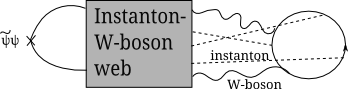
Figure 1: Calculating $\langle\tilde{\psi}\psi\rangle$

At the next step we assume that there is the web of interacting particles of two types between the operator insertion and the first loop which can braid providing the torus knots $T_{n,m}$ if we have $n$ propagating particles of one type and $m$ propagating particles of another type. Since we have prepared CS theory in CY space from the first loop in the external fields the ends of the propagating particles picture the torus knot in $S^{3}$ inside CY. From the viewpoint of the second loop with the operator inserted we evaluate the contribution to the condensate from the ”tadpole” connected to the loop by some web involving particles of two types. The knot invariants count the entropy of the web with fixed two quantum numbers which are attached to the loop in the external field. Equivalently, it can be thought as the particular entropic factor in the condensate of the bilinear operator.

In our case we have the loop of the antifundamental in the external graviphoton field and the loop of the fundamental with the inserted bilinear operator due to the derivative in the same external field. Due to the inverse geometric transition the loop of antifundamental provides the $SU(N)$ CS action in CY when the rank of the group is $n\propto\frac{m_{a}}{\epsilon}$ which is counterpart of the QED case above. The insertion of the fermionic bililear and the loop of antifundamental are connected by the instanton-W-boson web with electric and instanton charges $(n,m)$ which pictures the torus knot at the antifundamental side. From the viewpoint of the fundamental we evaluate the condensate of the bilinear in the external field taking into account the tadpole of the antifundamental connected by the W-boson-instanton web. The configuration of the web has some peculiarities, for instance, one has to have in mind that instantons are almost sitting at the top of each other in $C^{2}$. The multiplicity of the web yields the entropic factor in the condensate.

One more inspiration from the non-SUSY case goes as follows. Remind that the effective action QCD yielding the condensate in the first quantized representation as the weighted sum of the vev of Wilson loops over the arbitrary contours $C$

$$\frac{dS_{eff}}{dm}=\frac{d}{dm}\sum_{\mathcal{C}}e^{-mL(C)}e^{i\Phi(C)}\langle W(\mathcal{C})\rangle=\langle Tr\frac{1}{(D-m)}\rangle$$ (1)

where the electric Wilson loops or the resolvent of the Dirac operator are evaluated in the instanton-anti-instanton ensemble where $L(C)$ is the length of the trajectory and $\Phi(C)$ is the spin factor. When we consider the loop connected by the web with the local operator we can use the first quantized picture for loop hence effectively in this case one evaluates the weighted correlators of the Wilson loops with the local operator averaged over the shape of loop and over the moduli space of the web. In our case we could have in mind similar representation in terms of the sum over the averaged correlators of supersymmetric Wilson loops with local operator. .

The paper is organized as follows. In Section 2 we review the duality between the instantons and the torus knots found in [7] for the superpolynomials for the $T_{n,nk+1}$ series of the torus knots. In Section 3 we summarize the different ways to get the HOMFLY polynomials for the generic $T_{n,m}$ knots. In Section 4 we explain how the knot invariants can be obtained from SU(2) SQCD and clarify the meaning of the $(n,m)$ quantum numbers of the knot as the electric and instanton charges. In Section 5 we argue that the condensate can be obtained from the 5d theory with the fractional coefficient $k=m/n$ in front of the 5d CS term. Different counting problems yielding the knot polynomials are compared in Section 6. Also in this section we will discuss various interpretations of knot polynomials. The findings of this paper and the open questions are presented in the Conclusion.

2 Instanton - torus knot duality

In this Section we summarize the key observations from [7]. Five-dimensional supersymmetric QED consists of vector field $A_{A}$, four-component Dirac spinor $\lambda$ and Higgs field $\phi$, all lying in the adjoint representation of $U(1)$. The Lagrangian reads as follows:

$$\mathcal{L}=-\frac{1}{4g^{2}}F_{AB}F^{AB}+\frac{1}{g^{2}}(\partial_{A}\phi)^{2}+\cfrac{1}{g^{2}}\bar{\lambda}\gamma^{A}\partial_{A}\lambda$$ (2)

$\gamma^{A},A=1,...,5$ are five-dimensional gamma matrices. Since the adjoint action for the $U(1)$ group is trivial, this is a free theory.

To introduce $\Omega$-background one can consider a nontrivial fibration of $\mathbb{R}^{4}$ over a torus $T^{2}$ [3],[28]. The six-dimensional metric is:

$$ds^{2}=2dzd\bar{z}+\left(dx^{m}+\Omega^{m}d\bar{z}+\bar{\Omega}^{m}dz\right)^{2},$$ (3)

where $(z,\bar{z})$ are the complex coordinates on the torus and the four-dimensional vector $\Omega^{m}$ is defined as:

$$\Omega^{m}=\Omega^{mn}x_{n},\qquad\Omega^{mn}=\frac{1}{2\sqrt{2}}\begin{pmatrix}0&i\epsilon_{1}&0&0\\ -i\epsilon_{1}&0&0&0\\ 0&0&0&-i\epsilon_{2}\\ 0&0&i\epsilon_{2}&0\end{pmatrix}.$$ (4)

In general if $\Omega^{mn}$ is not (anti-)self-dual the supersymmetry in the deformed theory is broken. However one can insert R-symmetry Wilson loops to restore some supersymmetry [28]:

$$A^{I}_{J}=-\frac{1}{2}\Omega_{mn}\left(\bar{\sigma}^{mn}\right)^{I}_{J}d\bar{z}-\frac{1}{2}\bar{\Omega}_{mn}\left(\bar{\sigma}^{mn}\right)^{I}_{J}dz.$$ (5)

The most compact way to write down the supersymmetry transformations and the Lagrangian for the $\Omega$-deformed theory is to introduce ’long’ scalars (do not confuse them with $\mathcal{N}=1$ superfields):

$$\Phi=\varphi+i\Omega^{m}D_{m},\qquad\bar{\Phi}=\bar{\varphi}+i\bar{\Omega}^{m}D^{m},$$ (6)

We can couple this theory to fundamental hypermultiplet, which consists of two scalars $Q$, $\tilde{Q}$ and two Weyl fermions $\psi$ and $\tilde{\psi}$ and characterized by two masses: $m$ and $\tilde{m}$, since $\mathcal{N}=2$ hypermultiplet is build from two $\mathcal{N}=1$ hypermultiplets with opposite charges. Now the bosonic part reads as:

$$\begin{split}\mathcal{L}_{m}=-\frac{1}{4g^{2}}F_{mn}F^{mn}+\cfrac{1}{g^{2}}(\partial_{m}\phi+F_{mn}\Omega^{n})(\partial^{m}\phi-F^{mn}\Omega^{n})+\\ \cfrac{1}{2}|D_{m}Q|^{2}+\cfrac{1}{2}|D_{m}\tilde{Q}|^{2}+\cfrac{2}{g^{2}}(i\partial_{m}(\Omega^{m}\bar{\phi}+\Omega^{m}\phi)+g^{2}(\bar{Q}Q-\bar{\tilde{Q}}\tilde{Q}))^{2}+\\ \frac{1}{2}|(\phi-m-i\Omega^{m}D_{m})q|^{2}+\frac{1}{2}|(\phi-\tilde{m}-i\Omega^{m}D_{m})\tilde{q}|^{2}+2g^{2}|\tilde{q}q|^{2}\end{split}$$ (7)

In what follows we will be interested in the condensate of the massless fundamental $<\psi\tilde{\psi}>$ from the 4D viewpoint which depends on the parameters of the model. Upon reduction to the 4d theory we have asymptotically free theory when $N_{F}\leq 2$ for U(1) theory and $N_{f}\leq 4$ for SU(2). We shall consider the different number of flavors which in some case correspond to the theory with Landau pole.

Since we shall count the BPS states it is necessary to remind the spectrum of BPS particles in the theory. The corresponding central charge involves the quantum numbers corresponding to the instantons, W-bosons and fundamentals [29]

$$Z=\frac{1}{g^{2}}n_{I}+n_{e}a+\sum_{i}n_{f_{i}}m_{f_{i}}$$ (8)

The instantons in 5d theory are particles which carry the charge corresponding to the conserved topological current

$$J=*TrF\wedge F$$ (9)

If we add to the action the CS term

$$S_{CS}=k\int A\wedge F\wedge F$$ (10)

it couples the topological charge to the gauge field. In particular, this term implies that the instanton particle with instanton charge $n_{I}$ carries the electric charge $n_{I}k$ hence the central charge can be written as

$$Z=(n_{e}+kn_{I})a+\frac{1}{g^{2}}n_{I}+\sum_{i}n_{f_{i}}m_{f_{i}}$$ (11)

There are also the dyonic instantons carrying the topological and electric charges which are unstable under the blowup into the tubular D2 brane. Generically particle carries quantum numbers $(n_{I},n_{e},n_{f})$.

In [7] the new instanton-torus knot duality has been formulated for the Omega-deformed $\mathcal{N}=1$ 5d SUSY QED on $S^{1}_{\beta}\times\mathbb{R}^{4}_{\Omega}$ with the Chern-Simons term at level $k$. It has been proved that the second derivative of the Nekrasov instanton partition function with respect to the masses of the hypermultiplets is the generating function for the superpolynomials of the torus $T_{n,nk+1}$ knots where $n$ is the instanton charge.

$$\left.\frac{e^{\beta M}}{(1+A)\beta^{2}}\frac{d^{2}Z_{nek}(q,t,m_{f},M,m_{a},Q,k)}{dM\,dm_{f}}\right|_{m_{f}\to 0,M\to\infty}\vskip 6.0pt plus 2.0pt minus 2.0pt\\ =\sum_{n}Q^{n}(tq)^{n/2}P_{n,nk+1}(q,t,A)$$ (12)

where $m_{a},m_{f},M$ are masses of three hypermultiplets in antifundamental ($m_{a}$) and fundamental representations ($m_{f},M$) and Q is the counting parameter for the instantons. The mapping between the parameters at the lhs and rhs goes as follows

$$t=\exp(-\beta\epsilon_{1})$$ (13)

$$q=\exp(-\beta\epsilon_{2})$$ (14)

$$A=-\exp(\beta m_{a})$$ (15)

$$Q=\exp(-\beta/g^{2})$$ (16)

It is worth to think that the information about the knot invariants is encoded in the UV properties of the condensate of the massless flavor since the heavy fundamental sets the UV scale M.

The duality implies that the summation over the instanton charge is translated into summation over the particular series of the torus knots parameterized by the single integer - instanton charge. Certainly one could expect the double sums over generic torus knot $T_{n,m}$ and we shall demonstrate later that the double sum over the torus knots corresponds to the summation over the instanton and electric charges at the gauge theory side. It will be clear that the role of heavy flavor in [7] was to select the particular value of the electric charge and instead of a bit artificial procedure in Abelian theory it is more natural to embed the whole picture in SU(2) SQCD when the instanton and W-bosons enter at the equal footing.

In the unrefined case we expect the representation of the HOMFLY invariants in terms of the vev of electric Wilson loops in 3d CS theory and it is desirable to recognize this viewpoint as well. Saying a bit differently the question can be formulated as ”Where knots are located?”. The answer to this question would explain the CS representation of the HOMFLY invariants. We shall present the arguments that the knots are represented by the intersection of M2 branes representing the BPS states with several quantum numbers with the branes emerging through the inverse geometric transition. Another picture is provided by the string web ending at the 5-brane web. The knot invariants count the spin and flavor content of the instanton-W-boson web. We shall also explain the origin of the AGT type relation between the torus knot invariants and conformal blocks in q-Liouville theory observed in [7].

It is also instructive to recall [7, 8] that the differentiation with respect to the heavy mass can be equally thought of as an insertion of the operator $\exp(-\beta\Phi)$. Operator $\Phi$ is not quite the same as adjoint Higgs field since the later is not annihilated by Omega-deformed supersymmetry:

$$Q_{\Omega}\phi=\Omega^{m}A_{m}$$ (17)

and we require $\Phi$ to be Q-closed: $Q_{\Omega}\Phi=0$. In appendix B we will argue that the proper realization of chiral ring operator in the Omega-deformed theory is a lump of a brane-antibrane system. In what follows we substitute operator $\exp(-\beta\Phi)$ by a Lagrangian brane which will be useful to apply different dualities and geometric transitions.

3 Summary: condensates versus HOMFLY polynomials

In the previous paper [7] we focused at the superpolynomials of the torus knots which measure the response of the condensate of the massless flavor on the UV scale introduced by the particular operator in the theory with $N_{f}=2$ or in the $N_{f}=3$ with one heavy flavor. To some extend this corresponds to the evaluation of instanton contribution to the anomalous dimension of the bilinear operator. However it is interesting to find the interpretation of the condensate itself in terms of the knot invariants. We will consider the degeneration of the superpolynomials to the HOMFLY depending on two generating parameters in the self-dual unrefined case. It turns out that there are several ways to recognize the HOMFLY invariants of the torus knots in the evaluation of the condensates. They are complimentary and can be used to clarify the different aspects of the problem.

Let us summarize the different ways how the uncolored HOMFLY polynomials of the $T_{n,m}$ torus knots in the fundamental representation can be obtained and what is the meaning of the $(n,m)$ quantum numbers.

• We can use the representation of the superpolynomials of $T_{n,nk+1}$ knots in terms of the 5d abelian $N_{f}=3$ gauge theory with the integer CS term [7] and consider the limit of self-dual $\Omega$ background $\epsilon_{1}+\epsilon_{2}=0$ . In this approach we can describe only $T_{n,nk+1}$ series and have one counting parameter $n$ which corresponds to the 4d instanton charge. The second electric charge is chosen to be equal nk+1 by hands.

• Another approach is suggested by the celebrated Jones-Rosso formula [32] for the colored HOMFLY-PT polynomial(see [33] for a nice review). We will argue that this representation corresponds to the $N_{f}=2$ theory without the additional operator insertions but with the fractional CS term. In this representation we shall obtain the $n$-instanton contribution to the condensate itself as the HOMFLY invariant of $T_{n,nk+1}$ knot when the fractional 5d CS term is $l=k+1/n$. Note that the denominator in the CS coupling is equal to the number of instantons. This approach does not allow to get the instanton sums but provide the additional framework for the evaluations of the separate terms in the instanton sum. We will describe this approach in Section 5.

• As we have mentioned above, instead of the insertion of the particular operator in $N_{f}=2$ theory we can consider the $N_{f}=2$ SU(2) theory supplemented by the Lagrangian brane with zero framing with some value of FI parameter $z$. To get the HOMFLY polynomials we make two step procedure. First, we consider the decoupling limit $1/g^{2}\rightarrow\infty$ in SU(2) theory when it effectively decouples into the product of two U(1) theories and pure 4d instantons decouple. However due to the additional Lagrangian brane we have the FI parameter which counts the instantons on the Lagrangian brane. Considering the derivative of the Nekrasov partition function in this case with respect to mass and expanding it into the double series $z^{m}Q^{n}$ we obtain the HOMFLY polynomials of the generic $(n,m)$ knots as the coefficients of the expansion. In this case parameter $z$ counts the 2d instantons while the parameter Q equals to $\exp(\beta a)$ and counts the number of W- bosons in the decoupling perturbative limit of SU(2) theory. In this approach we can say that HOMFLY polynomials provide the entropic factor in the condensate in the sector with the particular defect. We will develop this approach in Section 4.2

• We can embed the abelian theory under consideration into the SU(2) with $N_{f}=4$. Two masses of fundamentals are fixed by parameters of the $\Omega$-deformation one mass tends to zero and one mass is arbitrary. No Lagrangian branes and CS terms are needed in this framework. If we expand the derivative of the partition function into the double series $e^{m\beta a}Q^{n}$ corresponding to the expansion in the electric and 4d instantonic charges we get the HOMFLY polynomial for the generic torus knots. No decoupling of 4d instantons occurs since $Q=\exp(\beta g^{-2})$ is finite. This approach is described in Section 4.5. It is this picture which immediately explains the origin of relation with the q-Liouville conformal blocks via AGT relation observed in [7]

It is worth to make more comments concerning the place of the different knot invariants in the context of the evaluation of the condensates. It is known in QCD that main phenomena behind the chiral condensate formation is the collectivization of the individual fermionic zero modes in the instanton-antiinstanton ensemble. There is no possibility to get the exact answers in QCD case and one has to restrict himself by the effective approaches like the matrix models or low-energy theorems. The localization technique in SUSY QCD provides the tool to describe the collectivization of the zero modes in the holomorphic ensemble of interacting instantons in a rigorous way.

It is clear that the knot invariants provide the entropic factor to the condensate which corresponds to the counting of degeneracy of the instanton–W-boson web with fixed $(n,m)$ quantum numbers. This is the particular realization of the approach to the knot homologies suggested in [34]. The complete set of states with two quantum numbers can be read off from the string web diagram in the IIB approach to the 5d SUSY theory [16].The fixed numbers (n,m) correspond to the numbers of the F1 and D1 strings involved into the particular web. However there are many possibilities to get the BPS states with these quantum numbers due to the number of string junctions involved and the boundaries of the web selected.

This general picture can be also realized in the combinatorial description of the torus knot invariants [5, 35] when the knot invariants including the superpolynomials can be derived from the weighted random walks in the $n\times m$ rectangle above the diagonal. The each random path corresponds to the particular fixed point in the localization integral over the instanton moduli space. The sum over the random paths in the 2d Young diagrams can be mapped into the 3d Young diagrams when each path maps to the particular 3d Young diagram corresponding to the fixed point. It would be very interesting to identify the fixed points with the particular BPS states with three quantum numbers explicitly and we hope to discuss this issue elsewhere.

4 HOMFLY invariants from SU(2) SQCD

4.1 Why SU(2)?

In [7] we have shown that some limits of the torus knot invariants are related to the DOZZ factors in the q-deformed Liouville theory. This implies via the 5d AGT relation that the evaluation of the knot invariants is related to the $\Omega$-deformed 5d SU(2) SQCD. On the other hand the previous analysis was based on the abelian theory hence the relation between the abelian and nonabelian pictures deserves the explanation. This Section is devoted to this issue and we will argue that the derivation of the HOMFLY invariants and condensate of the massless flavor matches in two pictures.

To this aim let us remind the toric diagram (aka web of 5-branes in IIB picture) for the 5d SU(2) SQCD with some number of flavors. We can obtain the field theory either by considering this web of branes or by M-theory compactification on the corresponding Calabi-Yau threefold. These two pictures are related by ”9-11” flip and a chain of T-dualities. The diagram is presented at Fig. 2 and some symmetry corresponding to 90 degree rotation is present supplemented by the particular mapping of parameters. It the base-fiber duality in the geometrical engineering language [34] or the bispectral duality in the language of the integrable systems. It was discussed in the related framework in [20, 36] were the explicit formulae for the relation between the dual representations of the Nekrasov partition function were derived. The two Kahler parameters $\exp(-\beta a)$ and $\exp(-\beta/g^{2})$ get interchanged under the rotation. The partition function can be presented as the double sum in the instanton and electric charge numbers and the sum over instantons gets interchanged with the sum over gauge bosons.

Figure 2: $SU(2)$ theory with light fundamental and heavy antifundamental hypermultiplets and a Lagrangian brane

The Lagrangian brane on the internal horizontal line represents M5 brane wrapped around Lagrangian three-cycle in the Calabi-Yau: if we consider our toric Calabi-Yau as $T^{2}\times\mathbb{R}$ fibration over base $\mathbb{R}^{3}$, then this Lagrangian cycle is extended along $T^{2}$ and a line in the base $\mathbb{R}^{3}$ - see [37, 38, 39] for details. In IIB language it is represented by the semi-infinite D3 brane perpendicular to the brane-web. From the 5d field theory it looks like the 3d surface defect. Upon the reduction to four dimensions it becomes familiar semi-infinite D2 brane representing string (see [40] for a detailed discussion).

The toric diagram for SU(2) suggests two possible decoupling limits when one or another Kähler class vanishes. These limits correspond to $g^{2}\rightarrow 0$ and $a\rightarrow\infty$ respectively. In four dimensions one could say that two limits correspond to the approaching the perturbative regime. However, the picture in five dimensions is more involved. We can cut the horizontal line at the toric diagram (see Fig. 5 where we showed only one half) which corresponds to the decoupling of the 5d instanton particles from the partition sum and the product of two U(1) partition functions remain. Now the Coulomb modulus in SU(2) theory plays the role of the gauge coupling in the abelian theory and the W-bosons in the SU(2) theory play now the role of the abelian instantons. Moreover, the Lagrangian brane is placed on the external leg. On the other hand, it was argued in [40] that such decoupling corresponds to decoupling of 5d degrees of freedom and, therefore, the partition function of the configuration on the Fig. 5 equals to the partition function on the 3d defect represented by the surface defect. Therefore, we arrive at the kind of 3d/5d duality:

5d $\mathcal{N}=1$ Abelian theory with $N_{f}=2$ and Lagrangian brane $\leftrightarrow$ 3d $\mathcal{N}=2$ Abelian theory with $N_{f}=4$

Oppositely one can cut the vertical lines (see Fig 3) and obtain once again the product of two abelian partition functions where the nonabelain instantons get mapped to the abelian ones. Note that the antifundamental matter can be treated as the fundamental one in the abelian case. Therefore in the decoupling limit we find ourself with the product of two abelian theories with some matter content which depends on the matter content in the initial SU(2) theory.

Figure 3: Two $U(1)$ theories as a limit from $SU(2)$ theory

How the decoupling procedure can be applied to the our study? First note that there are two issues which makes our case a bit more involved. There is non-vanishing 5d CS term in our Largangian which makes the toric diagram asymmetric (see Fig. 4) . Therefore there is the possibility to make the naive cut of the horizontal line only which yields the abelian factors with the different CS terms. Secondly when considering the knot invariants we have to consider the abelian theory with three flavors one of which plays the role of the ”regulator” . It can be substituted by the operator $\exp(-\beta\phi)$ with the ”long ” scalar which tells that the decoupling of the heavy flavor is incomplete in the spirit of the example considered in [41].

Figure 4: Pure gauge $SU(2)$ theory with the CS term at level 2

4.2 Back to abelian theory with Lagrangian brane

In terms of the toric diagrams the additional heavy flavor is realized in terms of the Lagrangian brane attached to the vertical line in the toric diagram. The field theory interpretation of this Largangian brane deserves the separate study since its interpretation is different compared to the branes attached to the horizontal or external leg. To some extend it mimics the single excited W-boson in the SU(2) corresponding to the $\exp(-\beta\phi)$ which has such remnant in the U(1) theory. Hence the decoupling in this toric diagram for SU(2) theory supplemented by the Lagrangian brane provides the explanation of the relation between the torus knot invariants and the vev of the particular observable in the q-deforned Liouville theory.

The realization of the knot invariants in terms of the SU(2) SQCD supplemented by defect is useful for the interpretation in terms of the instanton ensemble. In the abelian case the point-like instanton solution is purely defined and need for some regularization via non-commutativity or blow-ups at some points. In SU(2) case it is much simply to think about instantons and the decoupling $a\rightarrow\infty$ limit means that we effectively are in the perturbative regime with instantons and the single electric W-boson excitation. It is this series of terms in the double sum representation of the Nekrasov partition function for SU(2) SQCD with $N_{f}=2$ is intimately related with the torus knot invariants.

Figure 5: $SU(2)$ theory with a Lagrangian brane with zero framing after sending $1/g^{2}\rightarrow\infty$. Dot indicates preferred direction.

Now let us compute the condensate of the massless hypermultiplet in case of perturbative $SU(2)$ theory supplemented with the Lagrangian brane - Fig. 5.

The full partition function reads as:(see A for a very brief introduction to the topological vertex):

$$Z=\sum_{\lambda\mu\nu\alpha}(-Q_{c})^{|\lambda|}(-Q_{a})^{|\alpha|}(-Q_{m})^{|\mu|}C_{\nu\mu\lambda}(t,q)C_{\emptyset\mu^{t}\emptyset}(q,t)C_{\emptyset\alpha\lambda^{t}}(q,t)C_{\emptyset\alpha^{t}\emptyset}(t,q)s_{\nu}(-z\sqrt{q})$$ (18)

It is convenient to normalize the partition function:

$$Z_{inst}=\cfrac{Z}{Z(Q=0)}$$ (19)

Then the condensate has the following expansion:

$$\langle\tilde{\psi}\psi\rangle_{LB}=\cfrac{\partial Z_{inst}}{\partial m_{f}}\biggl{|}_{m_{f}=0}=\sum_{n,m}Q_{c}^{n}z^{m}P_{n,nk+m}(A,q,t)$$ (20)

$$P(A,q,t)_{n,nk+m}=$$ (21)

$${\sum_{\lambda:|\lambda|=n}\cfrac{t^{(k+1)\sum l}q^{(k+1)\sum a}(1-t)\prod^{0,0}(1+Aq^{-a^{\prime}}t^{-l^{\prime}})\prod^{0,0}(1-q^{a^{\prime}}t^{l^{\prime}})}{\prod(q^{a}-t^{l+1})\prod(t^{l}-q^{a+1})}\times}$$

$${Coef_{z^{m}}M(z)}$$

where $M(z)$ is the contribution from the Lagrangian brane with zero framing:

$$M(z)=\prod_{j=1}^{l(\lambda)}\cfrac{1-zt^{j-1}q^{\lambda_{j}}}{1-zt^{j-1}}$$ (22)

This expression has remarkable properties:

• At $m=1$ we recover the previous formula for a superpolynomial for $(n,nk+1)$ torus knot.

• It gives a polynomial in $A,q,t$ with integer positive coefficients if $gcd(n,nk+m)=1$. Unfortunately, we can not prove this statement rigorously.

• At $k=0$, $P_{n,m}=P_{m,n}$.

• At $t=1/q$ it gives correct HOMFLY polynomial for $(n,nk+m)$ torus knot. We will prove this fact in the appendix D

• However, in general, it does not reproduce conventional superpolynomial. Another problem is that the representation in terms of three numbers $n,k,m$ is redundant. Again, for general $\Omega$-deformation we will obtain different answers for the same knot if we choose $n,k$ and $m$ differently. Nonetheless, in the unrefined case the resulting expression does not depend on the choice of $n,k,m$.

Also, let us note that we could have placed the Lagrangian brane on the leg between $Q_{c}$ and $Q_{f}$. In this case we would get $\tilde{M}(z)$ instead of $M(z)$:

$$\tilde{M}(z)=\prod_{i=1}^{l(\lambda^{t})}\cfrac{1-zq^{i-1}t^{\lambda^{t}_{i}}}{1-zq^{i-1}}$$ (23)

It is easy to check that it will again lead to the HOMFLY polynomial, but in different normalization, however.

In fact, explicit formula for the superpolynomial of $(n,m)$ torus knot is known in mathematical literature[6]:

$$P^{(n,m)}=\sum_{|\lambda|=n}\cfrac{q^{2\sum a}t^{2\sum l}\prod^{0,0}(1+Aq^{-a^{\prime}}t^{-l^{\prime}})(1-q^{a^{\prime}}t^{l^{\prime}})}{\prod(q^{a+1}-t^{l})(t^{l+1}-q^{a})}\times$$ (24)

$$\sum^{SYT}_{ofshape\ \lambda}\cfrac{\prod_{i=1}^{n}\chi_{i}^{S_{m/n}(i)}(1-qt\chi_{i})}{\prod_{i=1}^{n-1}(1-\chi_{i})(1-qt\frac{\chi_{2}}{\chi_{1}})...(1-qt\frac{\chi_{n}}{\chi_{n-1}})}\prod_{1\leq i<j\leq n}\cfrac{(\chi_{j}-q\chi_{i})(\chi_{j}-t\chi_{i})}{(\chi_{j}-\chi_{i})(\chi_{j}-qt\chi_{i})}$$

where

$$S_{m/n}(i)=\lfloor\cfrac{im}{n}\rfloor-\lfloor\cfrac{(i-1)m}{n}\rfloor$$ (25)

The second factor is a sum over standard Young tableaux of shape $\lambda$: each tableaux is a Young diagram where each box is assigned a number from $1$ to $n$ in such a way that if we travel upwards or rightwards the numbers decrease. For each $i$ there is a box $\square_{i}$ and $\chi_{i}$ equals to $q^{a^{\prime}}t^{l^{\prime}}$.

We see that this quite complicated factor corresponds to the contribution of the defect responsible for superpolynomial. Unfortunately we can not identify this defect in the refined case precisely however in the self-dual $\Omega$-background it degenerates to the conventional Lagrangian brane.

4.3 Stable limit

Let us consider the limit of large Chern-Simons coupling $k\rightarrow\infty$. In this regime instantons die out and contributions from fundamental and antifundamental matter will factorize.

On the other hand, it was conjectured in [22] that if we consider the so-called stable limit $n\rightarrow\infty$ of the superpolynomial $\mathcal{P}_{n,m}$ we will obtain unknot colored in the symmetric representation $[m]$:

$$\lim_{n\rightarrow\infty}\mathcal{P}_{n,m}=\mathcal{P}_{unknot}^{[m]}$$ (26)

Now we will show that there is an analogue of this relation in our picture . Indeed, if we assume $q,t<1$, only $\lambda=\varnothing$ gives non-zero contribution in eq. (21). Fundamental hypermultiplet produces simple perturbative contribution

$$N_{f}=\prod_{i=1,j=1}^{\infty}(1-\exp(-\beta m_{f})q^{i-1}t^{-j})$$ (27)

which we will discard. Let us look closely at antifundamental hypermultiplet and Lagrangian brane - see Fig. 6. As in the previous sections, we will concentrate on instanton part of the partition function. However, in this case we will divide by $Z(z=0)$.

Figure 6: Stable limit. Dot indicates preferred direction.

This is nothing else than the familiar Ooguri-Vafa geometry which indeed produces colored HOMFLY in the unrefined case[9]: the partition function

$$Z^{unrefined}=\sum_{m}H_{m}(A,q)z^{m}$$ (28)

is the sum of HOMFLY polynomials $H_{m}(A,q)$ for unknot colored in symmetric representation $[m]$. Since we have only one Lagrangian brane we obtain only symmetric representations.

In the refined case the situation is a bit more subtle, since the answer depends on the choice of preferred direction[42]. Moreover, there are certain problems with superpolynomial not in the fundamental representation - see [33] for discussion. Surprisingly, if we carefully trace the contribution of the brane, our choice of preferred direction will rather lead us to superpolynomial in totally antisymmetric representation $1^{m}$  :

$$Z^{refined}=\prod_{i=1}^{\infty}\cfrac{1-zt^{i-1}}{1+Az\sqrt{q}t^{i-1/2}}$$ (29)

Therefore, we can write down a relation similar to the eq.(26):

$$\lim_{k\rightarrow\infty}\cfrac{Z(A,q,t,z,Q)}{Z(A,q,t,z=0,Q)}=\sum_{m}z^{m}P_{unknot}^{1^{m}}(A,q,t)$$ (30)

4.4 Vortex counting and Lagrangian brane

As was shown in [40] a Lagrangian brane corresponds to a surface operator on the gauge theory side and vortex counting in a 3d theory on this defect matches with the topological vertex computation in the Nekrasov-Shatashvili limit $t\to 1$. So it is instructive to find the expressions for torus knot polynomials directly from vortex counting. In our case we have a three-dimensional $\mathcal{N}=2$ abelian Higgs model on $R^{2}\times S^{1}$ with the addition of one fundamental chiral multiplet that corresponds to 5d vector multiplet and two anti-fundamental ones which comes from 5d fundamental and anti-fundamental hypermultiplets. The parameters for the matter multiplets can be read off from the brane construction of a surface operator in 4d :

Figure 7: The brane construction of a surface operator in type IIA string theory.

We also introduce the Omega-background parameter $q=\exp({-\beta\epsilon})$. The result for the vortex partition function is the following:

$$Z(z,q;Q_{c},Q_{m},A)=\sum_{m=0}^{\infty}\frac{\prod_{j=0}^{m-1}(1-Q_{m}q^{j})\prod_{j=0}^{m-1}(1+AQ_{c}q^{j})}{\prod_{j=1}^{m}(1-q^{j})\prod_{j=0}^{m-1}(1-Q_{c}q^{j})}z^{m}$$ (31)

with a shift $Q_{c}\to q^{-1}Q_{c}$. Taking the derivative with respect to $m_{f}$ and the limit $m_{f}\to 0$ we obtain

$$\cfrac{\partial Z}{\partial m_{f}}\biggl{|}_{m_{f}=0}=\sum_{m=0}^{\infty}\frac{\prod_{j=0}^{m-1}(1+AQ_{c}q^{j})}{(1-q^{m})\prod_{j=0}^{m-1}(1-Q_{c}q^{j})}z^{m}=\sum_{m,n}H_{(m,n)}(A,q)z^{m}Q_{c}^{n}$$ (32)

The coefficients $H_{(m,n)}$ can be found easily from the expression above

$$H_{(m,n)}=\frac{1+A}{1-q}\sum_{k}q^{k(k+1)/2}\frac{[m+n-k-1]_{q}!}{[m]_{q}[n]_{q}[k]_{q}![m-k-1]_{q}![n-k-1]_{q}!}A^{k}$$ (33)

where

$$[n]_{q}=\frac{1-q^{n}}{1-q}$$ (34)

It coincides with the result obtained using topological vertex and reproduces the known expressions for HOMFLY polynomials for coprime $(m,n)$. Also note that if $A=0$ then

$$(1-q)H_{(n,n+1)}=\frac{[2n]_{q}!}{[n]_{q}![n+1]_{q}!}$$ (35)

that is a $q$-deformed Catalan number.

Thus we obtain that knot polynomials also appear in the expansion of the condensate in 3d gauge theory. Now the winding numbers of a torus knot corresponds to the vortex parameter $z$ and the flavor parameter $Q$.

4.5 From Lagrangian brane to $SU(2)$ theory with four flavours

According to the AGT conjecture [43] and its 5-dimensional generalization [44, 45, 46, 20], the perturbative part of $SU(2)$ Nekrasov partition function is equal to three-point function in the Liouville theory or its q-deformed analogue. What is more, the insertion of a surface defect corresponds to the insertion of operator $V_{2,1}$ which is degenerate at level 2 . So we conclude that the perturbative partition function with a surface defect should be equal to the full $SU(2)$ partition function but with a very special choice of fundamental masses. Indeed such an equivalence was conjectured and checked in [47] by a virtue of two transformations on topological vertexes. Now we are going to review them.

The first one is usual open-closed duality: we can substitute a Lagrangian brane by a resolved conifold - see Figure 8.

Figure 8: Refind open-closed duality

Actually, if we consider general $Q_{r}$ we will arrive at the following contribution(the second ratio is a normalization by a perturbation contribution):

$$\prod_{i=1}^{l(\lambda)}\prod_{j=1}^{+\infty}\cfrac{(1-zQ_{r}t^{i-3/2}q^{\lambda_{i}-j-1/2})}{(1-zt^{i-1}q^{\lambda_{i}-j})}\cfrac{(1-zt^{i-1}q^{-j})}{(1-zQ_{r}t^{i-3/2}q^{-j-1/2})}$$ (36)

If we take $Q_{r}=q^{3/2}t^{1/2}$ we obtain exactly $M(z)$.

The second transformation is a construction of the projector onto trivial representations: suppose we have a diagram where two external lines intersect. Then we can add additional resolved conifold with a special Kähler class which will project representations on these two lines onto trivial ones - see Figure 9

Figure 9: Projector onto trivial representations

To sum up, we can obtain our ”almost superpolynomial” simply by $SU(2)$ theory with four flavours.

Figure 10: $SU(2)$ theory with four flavours

To obtain a more general picture for SU(2) theory we can consider not a single lagrangian brane, but a stack of $p$ branes. For this case we specialize to the unrefined limit. After doing the same procedure we obtain SU(2) theory [40] with two arbitrary mass parameters $q^{p}$ and $A$ (see fig. 11).

Figure 11: A more general picture in the unrefined limit

Note that we changed the order of matter multiplets on a toric diagram. This change can be considered as a replacement of a Lagrangian brane from a bottom leg to the top leg. It doesn’t affect the quantity we compute. In fact we already did this change when we were considering vortex counting.

Again let us compute the derivative of the free energy with respect to $Q_{m}$. The answer can be expressed in the following way

$$\cfrac{\partial Z(1,A,q^{p},Q_{m};q)}{\partial m}\biggl{|}_{m=0}=\sum_{(m,n)}\,H_{(m,n)}(A,q)H_{(m,n)}(q^{p},q)\,Q_{B}^{m}Q_{F}^{n}$$ (37)

where as above $H_{(m,n)}$ is a HOMFLY polynomial for torus knot. So the stack of branes simply gives another factor in the derivative which is a knot polynomial. This factor is trivial for a single brane.

Figure 12: Resolved conifold with two stacks of lagrangian branes

To relate our approach to the conventional CS representation we make a reversed geometric transition replacing a matter multiplet $A$ by an another stack of branes (see fig. 12)

Thus each stack of branes gives us a HOMFLY, which also has an interpretation as a Wilson loop operator for torus knot in Chern-Simons theory on $S^{3}$ which lives on each stack of branes with the parameters that coincide with the parameters in our case. The explanation of this fact is given in section 6.2.

Let us comment on the inverse geometrical transition. Geometric engineering of the fundamental matter implies $N_{f}$ blow-ups wth the corresponding Kahler moduli fixed by masses of fundamentals and antifundamentals. We aim to get CS Lagangian therefore we perform the inverse geometric transition and trade the Kahler moduli into the number of the topological branes wrapped around $S^{3}$. The relation between parameters goes as follows

$$Ng_{s}=m_{a}$$ (38)

where it is useful to perform the inverse transition with respect to the matter in the antifundamental. Having in mind the relation between the graviphoton field and the string coupling constant we get required parameter $A$ obeying the relation $A=q^{N}$. Note that to some extend similar relation can be seen even in the abelian theory in the external constant self-dual electromagnetic field $F$. The one-loop effective action is related to the large N limit of CS theory as follows

$$S_{eff}=\int_{0}^{\infty}dse^{-sk}\left(\frac{s/2}{sin(s/2)}\right)^{2}=logZ_{CS}(N\rightarrow\infty,k,S^{3})$$ (39)

where $k=\frac{m^{2}}{2eF}$ [27]. We can consider this case as the phenomena of the same nature having in mind the rank-level duality. However it is important to investigate the inverse transition in more detailes. In particular in the context of the knot invariants it is interesting to look at the interference of the inverse transitions performed with the several flavors.

4.6 Reduction to D=4 theory

Let us discuss reduction to the four dimensions in the framework of the $SU(2)$ theory. In D=5 we have the W-boson and instanton particles propagating in the loop. Both of them correspond to M2 branes wrapped around the base or fiber cycles. As was shown in [48] the one-loop contribution amounts to the instanton series in D=4 theory where the double sum in electric and instanton charges in D=5 gets reduced to the single sum in instanton charge in D=4. Since the HOMFLY polynomial measures the degeneracy of the states with $(n_{I},n_{e})$ quantum numbers this reduction implies that the partial resummation of the knot invariants takes place. Indeed, in order to take 4D limit, we send $\beta\rightarrow 0$ and $g\rightarrow 0$, but keeping the Coloumb parameter and masses finite:

$$\frac{\beta}{g^{2}}=\frac{1}{g_{4D}^{2}}=\operatorname{const}$$ (40)

$$a,m_{a},\epsilon=\operatorname{const}$$ (41)

The first equation reflects the fact that instantons propagating along the compact dimension become more familiar point-like instantons in four dimensions. To obtain particular $n-$instanton contribution $c_{n}$ to the condensate:

$$\langle\tilde{\psi}\psi\rangle_{4D}=\sum_{n}e^{-n/g_{4D}^{2}}c_{n}(\epsilon,m,a)$$ (42)

we need to perform the summation over all possible electric charges:

$$c_{n}(a,m_{a},\epsilon)=\lim_{\beta\rightarrow 0}\sum_{m=0}^{\infty}e^{-ma\beta}H_{n,m}(q,A)$$ (43)

As we send $\beta\rightarrow\infty$ terms with large $m$ become more and more relevant until the sum turn into Laplace-like transform. However, this is not exactly Laplace transform since $q=\exp(-\beta\epsilon)$ and $A=-\exp(\beta m_{a})$ depend on $\beta$ and approach 1 and -1 respectively. Because of this, we loose information about finite powers of $q$ and $A$ and the four-dimensional limit is not invertible. Nonetheless, it is natural to ask: is anything left from knot invariant?

The answer is straightforward: it is easy to see from the eq. (43) that the large $m$ behavior(stable limit) of $H_{n,m}$ is encoded into the analytic structure in variable $a$ of 4D instanton contribution $c_{n}$. Each pole at $-\alpha\epsilon$ corresponds to the term $q^{\alpha m}$ in HOMFLY polynomial $H_{n,m}$.

For example, let us consider two instantons. $H_{2,m}$ for $m>0$ reads as:

$$H_{2,m}=\cfrac{q(A+q-q^{-m}(Aq+1))}{q^{2}-1}$$ (44)

On the other hand, taking the 4D limit:

$$\cfrac{m_{a}+\epsilon}{2\epsilon a}+\frac{m_{a}-\epsilon}{2\epsilon(\epsilon-a)}$$ (45)

Two poles at $0$ and $\epsilon$ reflect $q^{0}$ and $q^{-m}$ terms respectively. We see that the four-dimensional limit is sensitive only to the large $m$ growth of the HOMFLY polynomial $H_{n,m}$. It means that the second winding of the knot become condensed. This “mathematical” condensation reflects physical condensation: in four-dimensions the fifth component of the vector potential $A_{5}$ condensates and joins the Higgs scalar.

5 Fractional 5d Chern-Simons term

In this Section we shall focus at the case of the fractional Chern-Simons term. It can be also considered as the fractional framing of the torus knot. Let us emphasize that the fractional CS term provides a bit different picture compared to the previous Sections and the level of the CS term is related in a different way with the type of the knot. The Jones-Rosso formula can be rewritten as (see Appendix C for details):

$$H^{(n,m)}_{\square}(A,q)=(-1)^{n-1}\cfrac{1-q^{n}}{q^{n}}\sum_{|\lambda|=n}{q^{(\frac{m}{n}+1)\sum(l-a)}\cfrac{\prod^{0,0}(1-q^{l^{\prime}-a^{\prime}})\prod^{0,0}(1+Aq^{a^{\prime}-l^{\prime}})}{\prod(q^{-l-1}-q^{a})(q^{-l}-q^{a+1})}}$$ (46)

The later formula strikingly resembles the instanton partition function of 5D $\mathcal{N}=1$ U(1) gauge theory on $\mathbb{R}^{4}_{\Omega}\times S^{1}_{\beta}$ in self-dual Omega deformation $\epsilon_{1}=-\epsilon_{2}$ with antifundamental matter of mass $m_{a}$ and fundamental matter of mass $m_{f}$ and with the CS term $m/n$ :

$$\cfrac{\partial\tilde{Z}^{inst}_{n}}{\partial m_{f}}\biggl{|}_{m_{f}=0}=(1+A)\beta\sum_{|\lambda|=n}{q^{(\frac{m}{n}+1)\sum(l-a)}\cfrac{\prod^{0,0}(1-q^{l^{\prime}-a^{\prime}})\prod^{0,0}(1+Aq^{a^{\prime}-l^{\prime}})}{\prod(q^{-l-1}-q^{a})(q^{-l}-q^{a+1})}}$$ (47)

with

$$q=\exp(-\beta\epsilon_{2}),\ A=\exp(\beta m_{a})$$ (48)

We will denote the partition function of this theory by $\tilde{Z}$. For unknot $(n,1)$ this formula gives the following result:

$$H^{(n,1)}_{\square}=\cfrac{1}{(1-q)q^{(n-1)/2}}$$ (49)

Now let us recall the following expression for the superpolynomial in the fundamental representation of $(n,nk+1)$ torus knot:

$$P(A,q,t)_{nk+1,n}=$$ (50)

$$\sum_{\lambda:|\lambda|=n}\large{\cfrac{t^{(k+1)\sum l}q^{(k+1)\sum a}(1-t)(1-q)\prod^{0,0}(1+Aq^{-a^{\prime}}t^{-l^{\prime}})\prod^{0,0}(1-q^{a^{\prime}}t^{l^{\prime}})(\sum q^{a^{\prime}}t^{l^{\prime}})}{\prod(q^{a}-t^{l+1})\prod(t^{l}-q^{a+1})}}$$

This expression can be obtained as an instanton partition function of 5D $\mathcal{N}=1$ U(1) gauge on $\mathbb{R}^{4}_{\Omega}\times S^{1}_{\beta}$ in general Omega-background, with the CS term k, with 2 fundamental matters and one anti-fundamental matter. Or, equivalently, with fundamental matter, antifundamental matter and chiral observable:

$$P(A,q,t)_{n,nk+1}=t^{-n/2}q^{-n/2}(1-t)(1-q)\cfrac{1}{1+A}\cfrac{\exp(\beta M)}{\beta^{2}}\cfrac{\partial}{\partial m_{f}}\cfrac{\partial}{\partial M}Z^{U(1)}_{n}(m_{f},m_{a},M)\biggl{|}_{m_{f}\rightarrow 0,\ M\rightarrow\infty}$$ (51)

or equivalently:

$$P(A,q,t)_{n,nk+1}=t^{-n/2}q^{-n/2}\cfrac{1}{1+A}\cfrac{\partial}{\partial(\beta m_{f})}\langle\exp(-\beta\phi)\rangle,\ m_{f}=0$$ (52)

We will denote the partition function of this theory by $Z$ without tilde in contrast to the theory with fractional CS term.

In order to obtain the HOMFLY-PT polynomial one need to take $t=1/q$. The relation between these two formulas reads as follows:

$$P_{n,nk+1}(A,q,q^{-1})=(-1)^{n}\cfrac{H^{n,nk+1}_{\square}(A,q)}{H^{n,1}_{\square}(A,q)}=(-1)^{n}(1-q)q^{(n-1)/2}H^{n,nk+1}_{\square}$$ (53)

while

$$H^{n,nk+1}_{\square}=(-1)^{n-1}\cfrac{1-q^{n}}{(1+A)q^{n}}\cfrac{\partial\tilde{Z}_{n}}{\partial(\beta m_{f})}\biggl{|}_{m_{f}\rightarrow 0}$$ (54)

From the above formulas it is possible to obtain various relations between condensates in different theories.

To complete this Section two remarks are in order. First, one could question about the generic instanton contribution when the instanton number does not equal to the denominator of the CS level. This question has been discussed in the math literature in [49]. It turns out that the generic situation is quite complicated and the instanton contributions can be expressed in terms of the superpositions of the colored HOMFLY polynomials. The second point to be mentioned concerns some analogy with the FQHE which can be described in two ways. One involves the fractional 3d CS term while in the second approach when the composite fermions are introduced the system of new effective degrees of freedom is described by the integer CS term. It seems that the discussion in this Section has some common features with that case.

Let us remind that the HOMFLY invariants can be obtained from the viewpoint of the instanton quantum mechanics. This representation corresponds just to the fractional CS approach. As we have discussed in [7] the 5d CS term induces the interaction between the instantons.The interaction is attractive and its strength is fixed by the coefficient in front of the CS term $k=m/n$ . In this approach the number of instantons is strictly correlated with the CS term and is equal to $n$. Since the interaction is attractive the falling to the center takes place and we have to investigate the fine structure of the $n$-instantons sitting at one point. The HOMFLY polynomials correspond to the counting of the $E=0$ states in the Calogero Hamiltonian [50, 51]. The special property of the rational CS term is that the corresponding Cherednik algebra has the finite-dimensional representation and the Calogero Hamiltonian is expressed in terms of the Dunkl operators $D_{i}$ which are generators of the Cherednik algebra. The HOMFLY polynomials can be considered as the special twisted character of the finite-dimensional representation which on the other hand is the twisted Willen-like index in the Calogero model counting the $E=0$ states with the proper weights.

6 Comments on the counting problems

In our paper we have argued that the HOMFLY polynomials of the torus knots count the multiplicities of the states with the fixed instanton and electric charges. Let us make a few remarks concerning its relation to another counting problems and possible applications.

6.1 Standard picture

According to [9] to get the HOMFLY polynomials from the type A topological strings one starts with the $T^{*}S^{3}$ geometry with N branes wrapped $S^{3}$. and add the Lagrangian brane wrapped the Lagrangian manifold $L_{K}$ intersecting $S^{3}$ along the knot K. The torus knot is the intersection of the singular surface

$$x^{n}=y^{m}$$ (55)

with the $S^{3}$. The Lagrangian brane has the topology $S^{1}\times R^{2}$ in CY manifold and is identified as the total space to the co-normal bundle to the knot K. Upon the geometric transition the N branes disappear and the resolved conifold supplemented the Lagrangian brane emerges. The Lagrangian brane lies in the fiber of the resolved conifold.

The HOMFLY polynomial corresponds to the counting of open M2 branes which end at the $L_{K}$ and have the topology of disc in the target and can be wrapped around the $P^{1}$ base. Two generating parameters count the spin of the open M2 brane and its momentum in the 11-th direction. Due to the singular fiber in the case of the torus knot contrary to the unknot calculation in [9] the counting of M2 branes is nontrivial due to the presence of the singularity and to some extend the single M2 brane acquires multiplicity. It was shown in [52] that this brane picture reproduces the approach in [35]. From the M-theory viewpoint the HOMFLY polynomial counts the M2 states ending on the M5 brane with geometry $R^{2,1}\times L_{K}$ where $R^{2,1}\in R^{4,1}$. Let us emphasize that in this conventional approach the knot K is fixed by the Lagrangian M5 brane added by hands.

6.2 Knots as boundaries of holomorphic instantons

In our picture the whole geometry contains the information about all torus knots and each knot corresponds to a particular sector of BPS spectrum. The knot is selected not by the additional $L_{K}$ brane but by BPS state itself. As we have discussed above the key point is the inverse geometric transition when we substitute the blow-up $S^{2}$ whose Kähler modulus is fixed by the mass of the antifundamental by the set of topological branes wrapped $S^{3}$ whose number is fixed by the mass. After all we count the multiplicities of M2 branes corresponding to the torus knot ending at the stack of topological branes. The representation of coloring of the knot corresponds to the way how the M2 brane ends at the stack. Note that we try to decouple the antifundamental and send its mass to infinity the rank of the gauge group tends to infinity as well. Hence even upon the naive decoupling of the heavy flavor we keep the information about the knot invariants. Note some similarity with the bootstrapping of the heavy flavor in [41] when the non-Abelian string was the remnant after the decoupling of the heavy flavor.

So it is tempting to relate each knot with the geometry of holomorphic instantons in the corresponding sector. As in [9] knots are seen in the picture where all branes are involved. So let’s consider a resolved conifold with two stacks of branes (see fig. 12). The contribution of holomorphic instantons into the partition function according to [9] is

$$Z_{inst}=\biggl{\langle}\exp\biggl{(}\sum_{\beta,s,R_{1},R_{2}}\sum_{n=1}^{\infty}\mathcal{N}^{\beta}_{s,R_{1},R_{2}}\frac{q^{ns}}{n(1-q^{n})}Q_{\beta}^{n}\,Tr_{R_{1}}U^{n}Tr_{R_{2}}V^{n}\biggr{)}\biggr{\rangle}_{CS_{1},CS_{2}}$$ (56)

where $U$ and $V$ are the holonomies of a gauge fields in the representations $R_{1}$ and $R_{2}$ on two different stacks of branes over the boundaries of instantons and $Q_{\beta}$ is the Kahler parameter of a cycle $\beta$. $\mathcal{N}^{\beta}_{s,R_{1},R_{2}}$ are integer coefficients that counts the degeneracies of BPS states with a given spin $s$ and which transform in the representations $R_{1}$ and $R_{2}$ under a $U(p)_{i}$ symmetries on the branes. Now consider an instanton that warps $m$ times around $Q_{B}$ cycle and $n$ times around $Q_{F}$ cycle. It also warps $(m,n)$ cycle on a torus in the fiber of the toric diagram. So it’s boundary also warps $(m,n)$ cycle on a torus on a Lagrangian branes. In this way we have a knot on $S^{3}$ and the contribution of this holomorphic instantons into our Chern-Simons theory appears with observables associated with a corresponding torus knots. Now if we take the derivative with respect to the mass, take the limit $m\to 0$ and expand the result over $Q_{B}$ and $Q_{F}$ then the coefficient in front of $Q_{B}^{m}Q_{F}^{n}$ for coprime $(m,n)$ can be expressed in the following way:

$$\frac{1}{1-q}\sum_{k,s,R_{1},R_{2}}^{\infty}k\,\mathcal{N}^{m,n,k}_{s,R_{1},R_{2}}q^{s}\,\langle Tr_{R_{1}}U^{n}\rangle\langle Tr_{R_{2}}V^{n}\rangle$$ (57)

The exponent disappeared since the partition function becomes trivial in the limit $m\to 0$. The form of this expression explains why do we obtain knot polynomials in the expansion. However it does not explain why in the case at hand only the fundamental representations contribute and does not give us the coefficient in front of the polynomials. For that we have to know the BPS states degeneracies $\mathcal{N}^{\beta}_{s,R_{1},R_{2}}$ explicitly.

After doing a geometric transition back to the $SU(2)$ picture we can express the coefficients of torus knot polynomials in terms of closed BPS states degeneracies. Indeed, the closed topological string free energy can be expressed as [10]

$$F=\sum_{m,n,p,l,r,s}\sum_{j_{L}}\sum_{k=1}^{\infty}\frac{(-1)^{2j_{L}}\mathcal{N}_{m,n,p,l,r,s}^{j_{L}}(q^{-2kj_{L}}+...+q^{2kj_{L}})}{k(q^{k/2}-q^{-k/2})^{2}}Q_{B}^{km}Q_{F}^{kn}Q_{m1}^{kp}Q_{m2}^{kl}Q_{m3}^{kr}Q_{m4}^{ks}$$ (58)

In the case of mass parameters $1$, $q$, $-A$, $Q_{m}$ the quantity we compute is just the derivative of it with respect to mass $m$ in the limit $m\to 0$ since the partition function goes to $1$ in this limit. If we consider the coefficient in front of $Q_{B}^{m}Q_{F}^{n}$ in this sum for coprime $(m,n)$ then there is only the contribution from the terms with $k=1$ and we obtain (up to an irrelevant factor)

$$H_{(m,n)}=\sum_{p,l,r,s}\sum_{j_{L}}\frac{(-1)^{2j_{L}}\mathcal{N}_{m,n,p,l,r,s}^{j_{L}}(q^{-2j_{L}}+...+q^{2j_{L}})}{(q^{1/2}-q^{-1/2})^{2}}l(-A)^{p}q^{r}$$ (59)

So all the coefficients of the HOMFLY polynomial for torus knot $(m,n)$ can be expressed in terms of $\mathcal{N}_{m,n,p,l,r,s}^{j_{L}}$.

6.3 View from IIB

Let us consider the corresponding counting problem in the IIB description. The particles are represented by the string web involving the $(p,q)$ strings. The rules of interactions in the web and the attaching of the string web to the 5-brane web are formulated in [16, 17] and it was argued that there are also the string strips corresponding to the strings located within 5 branes and bound states of webs and strips when the strip escapes from the hosting 5-brane. The knot polynomial in IIB counts the number of the different string webs with the fixed boundary condition of the string web at the 5-brane web. The counting of the spin content of the particles corresponding to the web has been discussed in [53] using the results from [54]. It was shown that the spin content of the particles represented by web fits with the expected dimension of the moduli space [54].

Note that there is some subtle issue concerning the role of the extended states in the physical space. The states with several quantum numbers can blow up and their stability is supported by the angular momentum. In the IIB case the dyonic instanton is represented by the D3 brane which can be considered as the blow-up of the string web. The $(n,m)$ quantum numbers are encoded in the particular solutions in the D3 brane worldvolume theory [18]. The total D3 brane charge should vanish hence it should have the closed worldvolume and can be thought of as the $D3-\bar{D3}$ bound state with the fixed electric and instanton charges $(p,q)$. It has the topology of $T^{2}$ in $\mathbb{R}^{4}\times S^{1}$ where radius of one circle equals to $\beta$ while the second comes from the blow-up of the string-web and its radius equals to

$$R^{2}\propto nm$$ (60)

The D3 brane do not shrink to the string due to the angular momentum supported by the fields on its worldvolume. In the physical space-time it corresponds to the closed dyonic loop.

The HOMFLY polynomial $P_{n,m}(A,q)$ depends on two generating parameters $(A,q)$ and let us remind their physical meaning . The q-parameter counts the angular momentum of the state in the self-dual $\Omega$ background, while as was shown in [7] the parameter $A$ counts the effects of the antifundamental mass. The string web with or without blow-up has evident similarities with the realization of HOMFLY as the weighted sum over the Dyck paths above the diagonal in the $(n,m)$ rectangle [5]. The q-grading corresponds to the area under the path. If we assume web blow-up the spin of the dyonic instanton is the product $nm$ and this product can be attributed to the boundary path without the corners. That is we conjecture that the boundary path gets mapped to the dyonic instanton itself. Any other non-boundary paths involve corners and nontrivial counting with respect to the $A$-grading. We can conjecture that these paths correspond to the generalization of the dyonic instantons in the theory with the fundamental and antifundamental matter.

The question if the blow up of the string web takes place and we could evaluate the knot polynomial in terms of the D3 worldvolume theory deserves further study. This question is important for the issue of the interpretation of the HOMFLY purely in the $R^{4}\times S^{1}$ space-time without appealing to the CY space.

6.4 Analogy with the baryonic vertex

Let us conclude this Section with the conjecture that the hidden torus knot structure can be expected in the configuration involving the multiple Skyrmion charges in QCD. To formulate the conjecture first remind the Skyrmion representation of the baryon found long time ago in [55]. The baryon was represented as the soliton state in the Chiral Lagrangian and its fermion statistics is due to the 5d Chern-Simons term. The coefficient in front of the CS term equals to the number of colors $N_{c}$.

In the holographic approach the Chiral Lagrangian is the worldvolume theory on the flavor D8 branes. There are two related ways to describe the baryon holographically. The baryonic vertex can be represented by the 5-brane wrapped around the compact cycle in the CY geometry [56]. The fundamental strings attached to the baryonic vertex are extended along the radial coordinate and correspond to the electric degrees of freedom at the boundary.

The baryon can be also represented as the instanton in the $SU(N_{f})_{L}\times SU(N_{f})_{R}$ 5d gauge theory on the flavor branes [59]. The baryon-instanton is extended along the physical time. It is useful also to have in mind the Atiyah-Manton representation of the Skyrmion from the instanton holonomy [60] when Skyrmion field is built from the components of the instanton connection in $D=5$. The formal realization has been recognized in terms of the instanton trapped inside the domain wall [61] in the particular 5d gauge theory with a few flavors which has a finite number of vacua.

The instanton interpretation suggests the interesting conjecture concerning the possible place of torus knots in the Skyrmion physics. The candidates for the torus knot quantum numbers are evident and we can speculate that the conventional charge B baryon at nonzero temperature is related to the $T_{B,N_{c}B+k}$ torus knot where the thermal circle plays the role of the KK circle in this case. The additional electric charge k can be related with the F1 strings attached to the baryons-instantons. In the case of the flavor gauge group the corresponding electric strings correspond to the vector mesons. To pursue the analogy further we have to suggest some place for the entropic factor which follows from degeneracy of the states with the fixed baryon and electric quantum numbers $(B,3B+k)$.

The analogy with the evaluation of the condensate goes as follows. Consider the chiral condensate which can be evaluated via the Casher–Banks relation in terms of the Dirac operator spectrum. Consider the quark loop with inserted bilinear operator and additional quark loop without the insertion. We could speculate that these two loops could be connected by the baryon-meson web analogous to the instanton-W-boson web in the SUSY case. The degeneracy in such web could play the role similar to the invariants.

One more remark is in order. In the SUSY case when we consider the torus knots with coprime $(n,m)$ the instantons are sitting on the top of each other. However when we analyze the $(n,nk)$ torus links the centering at one point disappear and the instantons form $n$ groups with $k$ instantons in each group [49]. Hence if we add just one unit of the electric charge to union of the $n$ links with linking number $lk_{i,j}=1$ the system gets topologically rearranged and become the single $(n,nk+1)$ torus knot. If the analogy with the Skyrmion physics works it would mean that if we start with the (B,3B) baryonic state and add the electric degree of freedom the state gets rearranged and the multi-baryon state becomes the single $(B,3B+1)$ torus knot.

Concluding this short comment on the analogy with Skyrmion physics and chiral condensate in QCD let us emphasize that the discussion above was a bit speculative however there are serious arguments to analyze this analogy further.

7 Conclusion

In this paper we discussed the role of the knot invariants in the gauge theories and have argued that the knot invariants count the entropy of the instanton–W-boson web involved into the condensate formation in SQCD. The picture is more transparent if the generic $T_{n,m}$ torus knots are considered and it was shown that the quantum numbers of the knot correspond to the instanton charge and electric charge of 5D particles. The key point is that the instanton–W-boson web with fixed two quantum numbers has some entropic factor due to the corresponding multiplicity which is captured by the torus knot invariants. We have seen such structure in the SU(2) SQCD or in simplified version of Abelian theory supplemented by the particular Lagrangian branes.

During the consideration we have seen that there are two representations of the HOMFLY invariants involving integer or fractional 5d CS terms. This seems to be parallel in many respects to the description of FQHE via composite fermions when the initial fermions identified as instantons get substituted by the composite fermions with attached disorder analogous to the dyonic instantons in our case. The relation with 4d and 2d FQHE seems to be deep and we shall postpone this issue for the separate publication. We shall focus at the hydrodynamical aspects of the FQHE liquid which is substituted by the hydrodynamical picture for the holomorphic instanton liquid [62].

In this paper we have focused at the 5d SUSY theory and made only a short trip to 4d theory when the knot invariants are encoded in the instanton contributions in the corresponding theory. More detailed analysis of the relation of the knot invariants with the different condensates in the 4d theories is certainly required . Since the low-energy effective actions in 4d theory in the Nekrasov-Shatashvili limit is governed by the quantum integrable system it is very interesting to recognize the knot invariants in the quantum integrable system. Another interesting issue concerns the theories with less amount of SUSY when the holomorphy is lost and instead of the instanton ensemble the instanton–anti-instanton ensemble has to be investigated. In this case we could expect a complicated linking phenomena responsible for the condensate formation.

In [8] we have observed the cascade of the different phase transitions in the ensembles of instantons and the torus knots. Our consideration suggests the possible stringy interpretation behind this phenomena. Indeed our evaluation of the condensate involves the calculation of the different correlators of the Wilson loops or Wilson loops with the local operators. When the number of W-bosons is large the instanton–W-boson web can be approximated by the surface and a kind of Gross-Ooguri phase transition [69] could take place which can be equivalently seen upon summation of the ladder diagrams in the perturbation theory [70].

Another interesting question concerns the application of the similar approach to the Schwinger process. At weak coupling in the worldline instanton formalism we localize at the particular trajectories in the Euclidean space-time. Usually one considers the single one loop $n$ the external field[71]. However one could question about the role of two bounce configuration or additional local operator apart from the bounce. The configuration of two bounces involving different flavors is suppressed by the additional exponential factor however twp loops could be related by the nontrivial instanton–W-boson web which produces the large entropic factor. The large entropic factor from the web could also emerge when we consider the Euclidean loop and the separate local operator.

The interesting question concerns the fate of the information stored in this web upon the materialization of Schwinger pairs after the Wick rotation to the Minkowski space. It could yield a interesting entanglement factor. In the holographic picture the Schwinger process requires the evaluation of the minimal surface [72](see also [73] for more recent discussion) probably with the additional operator insertion if the effect of the condensate on the pair production is considered. This corresponds to the stable limit of the torus knots. When we consider two Euclidean circles connected by the web the saddle point solution gets modified. Let us also emphasize that in the unrefined case corresponding to the self-dual external field in some signature there is no Schwinger pair production however in the refined case these nonperturbative effects are unavoidable.

Concerning more formal problems we could mention first the generalization to the colored HOMFLY polynomials. There are a few interesting questions related to these issues. It is necessary to recognize the physical interpretation of the generating parameters for the coloring. The natural candidate is the mass of the fundamental however the immediate inspection shows that it can not be literally true and more involved analysis is required. The knot polynomials with four gradings have been considered in [74]. From the instanton side in the colored case the centering of the instantons at one point is destroyed and instantons are collected in the several groups located at the different points in $R^{4}$ [49]. This suggests that the colored polynomials are related not to the condensates but to the topological correlators.

This problem can be also considered for the generic values of the masses of fundamentals and antifundamentals in SU(2) or higher rank theory. We expect that in the unrefined case the corresponding condensates are related to the combination of the products of the HOMFLY knot invariants. Indeed we have shown that each fermionic determinant dressed by $(n_{i},m_{i})$ numbers of instantons and W-bosons provides the HOMFLY invariant $P_{n_{i},m_{i}}(q,a_{i})$ where $a_{i}$ corresponds to the mass of the corresponding hyper. Hence the expected structure for the contribution in the $(n,m)$ sector is the product of the several HOMFLY invariants with the fixed value of the total instanton and electric charges.

The condensate can be considered as the derivative of the conformal block in the q-Liouville theory with respect to the parameter of the vertex operators. The interpretation of the double expansion of q-Liouville conformal block as the generating function for the HOMFLY polynomials is quite promising and should clarify the way of regular evaluation of the knot invariants in terms of the 2d conformal field theory.

Another immediate question concerns the recognition of the knot invariants in the integrability framework using duality we have found. The relation with integrability can be formulated, for instance, in terms of the corresponding XXZ spin chain and q-Liouville theory in the CY space or the Calogero model in the physical space. The Whitham hierarchy should control the dependence of the knot polynomials on the generating parameters. The several dualities known in the integrability framework should be recognized and used in the knot theory framework. As the simplest example remark that the $n\leftrightarrow m$ duality in the torus knot is the bispectral duality in the integrability framework. The generalization to the $SU(N)$ case with the different matter is expected to provide more general knot invariants. We shall discuss these issues elsewhere [75].

Appendix A The refined topological vertex

To establish some notations, let us very briefly review the topological vertex[76, 77] calculations. In physical terms, topological vertexes compute 5D Nekrasov partition function for the gauge theory living on a given web of $(p,q)$ 5-branes. In mathematical terms, they compute Gromov-Witten invariants for a given toric Calabi-Yau threefold.

The building block is a trivalent vertex - Fig. 13.

Figure 13: The topological vertex.

In order to compute the partition function one has to divide the web into such vertexes, put a Young diagram on each internal line and empty Young diagram on external lines and then sum over these diagrams. Each vertex contributes factor

$$C_{\mu\nu\lambda}(q)=q^{-\frac{k(\nu)}{2}}s_{\lambda}(q^{\rho})\sum_{\tau}s_{\mu^{t}/\tau}(q^{\rho+\lambda})s_{\nu/\tau}(q^{\rho+\lambda^{t}})$$ (61)

where $s_{\lambda}$ - Schur polynomials and $\rho_{i}=i-\frac{1}{2}$. We have used the following functions on a Young diagram $\lambda$:

$$||\lambda||^{2}=\sum_{i}\lambda^{2}_{i}$$ (62)

$$k(\lambda)=\sum_{i}\lambda^{2}_{i}-\lambda^{t\ 2}_{i}$$ (63)

Also, one has to take care of framing factors corresponding to internal lines[34]. Without going into details, we just say that each internal line contributes

$$f_{\nu}(q)=(-1)^{|\nu|}q^{\frac{k(\nu)}{2}}$$ (64)

to the power of line’s framing.

Also, we can add Lagrangian branes to a toric diagram. From physical viewpoint they are D3 branes transversal to the original brane-web. From mathematical viewpoint they correspond to relative Gromov-Witten invariants relative to a Lagrangian submanifold in the CY. If we place a stack of branes on an external leg, then we have to place a Young diagram $\mu$ on this leg and these Lagrangian branes contribute

$$s_{\mu}(-z_{1},-z_{2},\dots)$$ (65)

In [77], Iqbal, Kozcaz and Vafa generalized this beautiful and powerful technique to general $\Omega$-background:

$$C_{\mu\nu\lambda}(t,q)=(qt)^{-\frac{||\nu||^{2}+||\lambda||^{2}}{2}}t^{\frac{k(\nu)}{2}}P_{\lambda}(t^{-\rho},1/q,t)\sum_{\tau}(qt)^{\frac{|\nu|-|\tau|-|\mu|}{2}}s_{\mu^{t}/\tau}(t^{-\rho}q^{\lambda})s_{\nu/\tau}(q^{\rho}t^{-\lambda^{t}})$$ (66)

where $P_{\lambda}$ is MacDonald polynomial and

$$q=\exp(-\beta\epsilon_{1})$$ (67)

$$t=\exp(-\beta\epsilon_{2})$$

And the framing factor reads as:

$$f_{\nu}(t,q)=(-1)^{|\nu|}(tq)^{\frac{|\nu|-||\nu||^{2}}{2}}q^{+\frac{k(\nu)}{2}}$$ (68)

Now the vertex has no cyclic symmetry, and one has to choose preferred direction(see Fig. 14). Usually, the answer does not depend on the particular choice for closed amplitudes, but it is not always so for open amplitudes[77, 42].

Figure 14: The refined topological vertex. Dot indicates preferred direction.

For all known examples it reproduces Nekrasov instanton formulas. However, there are still a plethora of unaswered questions. For example, even before [77], in [78] Awata and Kanno proposed another version of refined vertex. Again, for all known closed amplitudes the Iqbal-Kozcaz-Vafa(IKV) and Awata-Kanno(AK) vertexes give the same answer. Nonetheless, we will use the IKV vertex with caution.

Appendix B Chiral ring and Lagrangian branes

Following [79] we will introduce generating function $Y(z)$

$$Y(z)=\exp\left(\sum_{n=1}\cfrac{z^{-n}}{n}\mathcal{O}_{n}\right)$$ (69)

for expectation values of chiral ring operators:

$$\mathcal{O}_{n}=\langle\exp(-n\beta\Phi)\rangle$$ (70)

One can show that in terms of instanton partitions $Y(z)$ reads as[80]:

$$Y(z)=\cfrac{1}{(1-z)}\cfrac{\prod_{\square\in\partial_{+}\lambda}(z-q^{a^{\prime}}t^{l^{\prime}})}{\prod_{\square\in\partial_{-}\lambda}(z-qtq^{a^{\prime}}t^{l^{\prime}})}$$ (71)

Let us show that this function is actually a wave-function for brane-antibrane system. We have seen that a single Lagrangian brane with zero framing on an external leg contributes factor

$$M(z)=\prod_{j=1}^{l(\lambda)}\cfrac{1-zt^{j-1}q^{\lambda_{j}}}{1-zt^{j-1}}$$ (72)

to the $U(1)$ instanton partition function.

Also, depending on the leg and framing we will arrive at either $M(z)$ - for brane, or $1/M(z)$ - for antibrane.

Figure 15: $U(1)$ theory with two Lagrangian branes on external legs. We should choose zero framing for the left brane and $+1$ for the right one

Actually, functions $Y(z)$ and $M(z)$ are not independent: they obey a very simple relation:

$$Y(z)=\cfrac{M(1/z)}{M(1/zt)}$$ (73)

The proof consists of a simple comparing which boxes in Young diagrams actually contribute the left hand side and right hand side.

To obtain a ratio of two $M$ functions, we can consider two Lagrangian branes(Fig. 15).

$$Z=\sum_{\lambda,\mu,\nu}(-Q)^{|\lambda|}C_{\emptyset\nu\lambda}(q,t)C_{\mu\emptyset\lambda^{t}}(t,q)f_{\lambda}(t,q)f_{\nu}(t,q)s_{\nu}(-z_{2}\sqrt{q})s_{\mu}(-z_{1}\sqrt{q})$$ (74)

Lagrangian branes contribute:

$$\cfrac{M(z_{1})}{M(z_{2})}$$ (75)

For $z_{2}=z_{1}t=zt$ we obtain exactly instanton part of $Y(1/z)$.

Since $Y(z)$ is the generation function for chiral ring operators, we conclude that these operators could be obtained by a brane-antibrane lump of size $\epsilon_{2}$.

Actually, we can invert (73):

$$M(z)=\prod_{i=0}^{\infty}Y(z^{-1}t^{-i})$$ (76)

Or in terms of chiral ring VEVs:

$$M(z)=\exp\left(\sum_{n=1}^{\infty}\cfrac{z^{n}t^{n}\mathcal{O}_{n}}{n(t^{n}-1)}\right)$$ (77)

Actually it is easy to generalize the above formulas to the $SU(N)$ case but we postpone this to the future work.

Appendix C Jones-Rosso formula

The Jones-Rosso formula for the HOMFLY-PT polynomial of $(n,m)$ torus knot colored in the representation $R$ reads as follows:

$$H^{(n,m)}_{R}(A,q)={\sum_{\lambda\in R^{\otimes n}}q^{\frac{m}{n}\sum_{\square\in\lambda}(a-l)}c_{R}^{\lambda}\chi_{\lambda}(p^{*})}$$ (78)

where:

• $R$ - Young diagram defining the representation

• $c_{R}^{\lambda}$ - Adams coefficients, defined by the action of the Adams operation on Schur polynomials $\chi_{\mu}(p)$:

  $$\chi_{\mu}(p^{(n)})=\sum_{\eta\in\mu^{\otimes n}}c_{\mu}^{\eta}\chi_{\eta}(p)$$ (79)

  In our notation we write arguments of Schur polynomials as power series polynomials $p_{k}=x_{1}^{k}+x_{2}^{k}+...$ and

  $$p^{(n)}_{k}=p_{nk}=x_{1}^{nk}+x_{2}^{nk}+...$$ (80)

• Finally, $p^{*}$ define the special choice of power series polynomials:

  $$p_{k}^{*}=\cfrac{(-A)^{k}-(-A)^{-k}}{q^{k}-q^{-k}}$$ (81)

Lets rewrite the Jones-Rosso formula (78) in a more explicit form. It is very-well known[81] that for the special choice of $p^{*}$ (81), Schur polynomials read as:

$$\chi_{\lambda}(p^{*})={q^{\sum a}\cfrac{\prod(1+Aq^{l^{\prime}-a^{\prime}})}{\prod(1-q^{a+l+1})}}$$ (82)

If we confine ourselves to the fundamental representation $R=\square$ then it is possible to obtain an explicit expression for the Adams coefficient[82]:

$$c_{\square}^{\lambda}={q^{\sum a}(1-q^{n})\cfrac{\prod^{0,0}(1-q^{l^{\prime}-a^{\prime}})}{\prod(1-q^{a+l+1})}}$$ (83)

Combining all the factors we obtain the following expression for the HOMFLY-PT polynomial in fundamental representation for $(n,m)$ torus knot(we omitted the trivial factor $(1+A)$):

$$H^{(n,m)}_{\square}=(1-q^{n})\sum_{|\lambda|=n}{q^{2\sum a}q^{\frac{m}{n}\sum(a-l)}\cfrac{\prod^{0,0}(1-q^{l^{\prime}-a^{\prime}})\prod^{0,0}(1+Aq^{l^{\prime}-a^{\prime}})}{\prod(1-q^{a+l+1})^{2}}}$$ (84)

Or equivalently:

$$H^{(n,m)}_{\square}(A,q)=(-1)^{n-1}\cfrac{1-q^{n}}{q^{n}}\sum_{|\lambda|=n}{q^{(\frac{m}{n}+1)\sum(a-l)}\cfrac{\prod^{0,0}(1-q^{a^{\prime}-l^{\prime}})\prod^{0,0}(1+Aq^{l^{\prime}-a^{\prime}})}{\prod(q^{-l-1}-q^{a})(q^{-l}-q^{a+1})}}$$ (85)

Appendix D Lagrangian brane and JR formula

Now let us show that the formula (21) in the unrefined case does indeed reproduce the JR expression. First of all, note that because of the factor $\prod^{0,0}(1-q^{l^{\prime}-a^{\prime}})$ only hook-shaped Young diagrams contribute.

$$\Young\cr\cr\cr&\cr$$

Figure 16: Hook-shaped Young diagram

Suppose that the hook-shaped diagram $\lambda$ has the horizontal ”arm” of length $w$. Then the vertical ”leg” has length $n-w+1$, since the total number of boxes is $n$. Chern-Simons term in the JR formula gives

$$q^{\frac{m}{n}\left(\sum a-\sum l\right)}=q^{mw-\frac{m(n+1)}{2}}$$ (86)

Whereas the contribution from Lagrangian brane:

$$M(z)=\cfrac{1-q^{w}z}{1-q^{w-n}z}$$ (87)

Therefore

$$Coef_{z^{m}}M(z)=q^{m(w-n)}(1-q^{n})$$ (88)

We see that apart from the normalization factor $q^{m(1-n)/2}$ these two expressions coincide.

sei,seimor

witten98s, gukov98s

tanzini1,tanzini2,no_ilw,tanzini15,litvinov1,litvinov2

References

- [1] V.A. Novikov, Mikhail A. Shifman, A.I. Vainshtein and Valentin I. Zakharov “Instanton Effects in Supersymmetric Theories” In Nucl.Phys. B229, 1983, pp. 407 DOI: 10.1016/0550-3213(83)90340-1
- [2] N. Michael Davies, Timothy J. Hollowood, Valentin V. Khoze and Michael P. Mattis “Gluino condensate and magnetic monopoles in supersymmetric gluodynamics” In Nucl.Phys. B559, 1999, pp. 123–142 DOI: 10.1016/S0550-3213(99)00434-4
- [3] Nikita A. Nekrasov “Seiberg-Witten prepotential from instanton counting” In Adv.Theor.Math.Phys. 7, 2004, pp. 831–864 DOI: 10.4310/ATMP.2003.v7.n5.a4
- [4] Mark Haiman “t, q-Catalan numbers and the Hilbert scheme” In Discrete Mathematics 193.1 Elsevier, 1998, pp. 201–224
- [5] E Gorsky “q, t-Catalan numbers and knot homology” In Zeta functions in algebra and geometry, 2012, pp. 213–232 arXiv:1003.0916
- [6] E. Gorsky and A. Neguţ “Refined knot invariants and Hilbert schemes” In ArXiv e-prints, 2013 arXiv:1304.3328 [math.RT]
- [7] A. Gorsky and A. Milekhin “Condensates and instanton - torus knot duality. Hidden Physics at UV scale”, 2014 arXiv:1412.8455 [hep-th]
- [8] K. Bulycheva, A. Gorsky and S. Nechaev “Critical behavior in topological ensembles”, 2014 arXiv:1409.3350 [hep-th]
- [9] Hirosi Ooguri and Cumrun Vafa “Knot invariants and topological strings” In Nucl.Phys. B577, 2000, pp. 419–438 DOI: 10.1016/S0550-3213(00)00118-8
- [10] Rajesh Gopakumar and Cumrun Vafa “On the gauge theory / geometry correspondence” In Adv.Theor.Math.Phys. 3, 1999, pp. 1415–1443 arXiv:hep-th/9811131 [hep-th]
- [11] Andrea Brini, Bertrand Eynard and Marcos Marino “Torus knots and mirror symmetry” In Annales Henri Poincare 13, 2012, pp. 1873–1910 DOI: 10.1007/s00023-012-0171-2
- [12] Hans Jockers, Albrecht Klemm and Masoud Soroush “Torus Knots and the Topological Vertex” In Lett.Math.Phys. 104, 2014, pp. 953–989 DOI: 10.1007/s11005-014-0687-0
- [13] Mina Aganagic, Marcos Marino and Cumrun Vafa “All loop topological string amplitudes from Chern-Simons theory” In Commun.Math.Phys. 247, 2004, pp. 467–512 DOI: 10.1007/s00220-004-1067-x
- [14] Sheldon H. Katz, Albrecht Klemm and Cumrun Vafa “Geometric engineering of quantum field theories” In Nucl.Phys. B497, 1997, pp. 173–195 DOI: 10.1016/S0550-3213(97)00282-4
- [15] Sheldon H. Katz and Cumrun Vafa “Matter from geometry” In Nucl.Phys. B497, 1997, pp. 146–154 DOI: 10.1016/S0550-3213(97)00280-0
- [16] Ofer Aharony, Amihay Hanany and Barak Kol “Webs of (p,q) five-branes, five-dimensional field theories and grid diagrams” In JHEP 9801, 1998, pp. 002 DOI: 10.1088/1126-6708/1998/01/002
- [17] Ashoke Sen “String network” In JHEP 9803, 1998, pp. 005 DOI: 10.1088/1126-6708/1998/03/005
- [18] Erik P. Verlinde and Marcel Vonk “String networks and supersheets”, 2003 arXiv:hep-th/0301028 [hep-th]
- [19] Naichung Conan Leung and Cumrun Vafa “Branes and toric geometry” In Adv.Theor.Math.Phys. 2, 1998, pp. 91–118 arXiv:hep-th/9711013 [hep-th]
- [20] Ling Bao, Elli Pomoni, Masato Taki and Futoshi Yagi “M5-Branes, Toric Diagrams and Gauge Theory Duality” In JHEP 1204, 2012, pp. 105 DOI: 10.1007/JHEP04(2012)105
- [21] Edward Witten “Quantum Field Theory and the Jones Polynomial” In Commun.Math.Phys. 121, 1989, pp. 351–399 DOI: 10.1007/BF01217730
- [22] Nathan M. Dunfield, Sergei Gukov and Jacob Rasmussen “The Superpolynomial for knot homologies”, 2005 arXiv:math/0505662 [math.GT]
- [23] Sergei Gukov, Albert S. Schwarz and Cumrun Vafa “Khovanov-Rozansky homology and topological strings” In Lett.Math.Phys. 74, 2005, pp. 53–74 DOI: 10.1007/s11005-005-0008-8
- [24] Mina Aganagic and Shamil Shakirov “Knot Homology and Refined Chern-Simons Index” In Commun.Math.Phys. 333.1, 2015, pp. 187–228 DOI: 10.1007/s00220-014-2197-4
- [25] Edward Witten “Fivebranes and Knots”, 2011 arXiv:1101.3216 [hep-th]
- [26] Davide Gaiotto and Edward Witten “Knot Invariants from Four-Dimensional Gauge Theory” In Adv.Theor.Math.Phys. 16.3, 2012, pp. 935–1086 DOI: 10.4310/ATMP.2012.v16.n3.a5
- [27] A. Gorsky and V. Lysov “From effective actions to the background geometry” In Nucl.Phys. B718, 2005, pp. 293–318 DOI: 10.1016/j.nuclphysb.2005.04.020
- [28] Nikita Nekrasov and Andrei Okounkov “Seiberg-Witten theory and random partitions”, 2003 arXiv:hep-th/0306238 [hep-th]
- [29]
- [30] Nathan Seiberg “Five-dimensional SUSY field theories, nontrivial fixed points and string dynamics” In Phys.Lett. B388, 1996, pp. 753–760 DOI: 10.1016/S0370-2693(96)01215-4
- [31] David R. Morrison and Nathan Seiberg “Extremal transitions and five-dimensional supersymmetric field theories” In Nucl.Phys. B483, 1997, pp. 229–247 DOI: 10.1016/S0550-3213(96)00592-5
- [32] Marc Rosso and Vaughan Jones “On the invariants of torus knots derived from quantum groups” In Journal of Knot Theory and its Ramifications 2.01 World Scientific, 1993, pp. 97–112
- [33] P. Dunin-Barkowski et al. “Superpolynomials for toric knots from evolution induced by cut-and-join operators” In JHEP 1303, 2013, pp. 021 DOI: 10.1007/JHEP03(2013)021
- [34] Sergei Gukov, Albert S. Schwarz and Cumrun Vafa “Khovanov-Rozansky homology and topological strings” In Lett.Math.Phys. 74, 2005, pp. 53–74 DOI: 10.1007/s11005-005-0008-8
- [35] Alexei Oblomkov and Vivek Shende “The Hilbert scheme of a plane curve singularity and the HOMFLY polynomial of its link” In Duke Math. J. 161.7 Duke University Press, 2012, pp. 1277–1303 DOI: 10.1215/00127094-1593281
- [36] Yegor Zenkevich “Generalized Macdonald polynomials, spectral duality for conformal blocks and AGT correspondence in five dimensions” In JHEP 1505, 2015, pp. 131 DOI: 10.1007/JHEP05(2015)131
- [37] Sergei Gukov, Amer Iqbal, Can Kozcaz and Cumrun Vafa “Link Homologies and the Refined Topological Vertex” In Commun.Math.Phys. 298, 2010, pp. 757–785 DOI: 10.1007/s00220-010-1045-4
- [38] Mina Aganagic, Albrecht Klemm and Cumrun Vafa “Disk instantons, mirror symmetry and the duality web” In Z.Naturforsch. A57, 2002, pp. 1–28 arXiv:hep-th/0105045 [hep-th]
- [39] K. Hori et al. “Mirror symmetry”, 2003
- [40] Tudor Dimofte, Sergei Gukov and Lotte Hollands “Vortex Counting and Lagrangian 3-manifolds” In Lett.Math.Phys. 98, 2011, pp. 225–287 DOI: 10.1007/s11005-011-0531-8
- [41] Davide Gaiotto, Leonardo Rastelli and Shlomo S. Razamat “Bootstrapping the superconformal index with surface defects” In JHEP 1301, 2013, pp. 022 DOI: 10.1007/JHEP01(2013)022
- [42] Hidetoshi Awata and Hiroaki Kanno “Changing the preferred direction of the refined topological vertex” In J.Geom.Phys. 64, 2013, pp. 91–110 DOI: 10.1016/j.geomphys.2012.10.014
- [43] Luis F. Alday, Davide Gaiotto and Yuji Tachikawa “Liouville Correlation Functions from Four-dimensional Gauge Theories” In Lett.Math.Phys. 91, 2010, pp. 167–197 DOI: 10.1007/s11005-010-0369-5
- [44] Hidetoshi Awata and Yasuhiko Yamada “Five-dimensional AGT Conjecture and the Deformed Virasoro Algebra” In JHEP 1001, 2010, pp. 125 DOI: 10.1007/JHEP01(2010)125
- [45] Can Kozcaz, Sara Pasquetti and Niclas Wyllard “A and B model approaches to surface operators and Toda theories” In JHEP 1008, 2010, pp. 042 DOI: 10.1007/JHEP08(2010)042
- [46] Ricardo Schiappa and Niclas Wyllard “An A(r) threesome: Matrix models, 2d CFTs and 4d N=2 gauge theories” In J.Math.Phys. 51, 2010, pp. 082304 DOI: 10.1063/1.3449328
- [47] Masato Taki “Surface Operator, Bubbling Calabi-Yau and AGT Relation” In JHEP 1107, 2011, pp. 047 DOI: 10.1007/JHEP07(2011)047
- [48] Albion E. Lawrence and Nikita Nekrasov “Instanton sums and five-dimensional gauge theories” In Nucl.Phys. B513, 1998, pp. 239–265 DOI: 10.1016/S0550-3213(97)00694-9
- [49] Pavel Etingof, Eugene Gorsky and Ivan Losev “Representations of rational Cherednik algebras with minimal support and torus knots” In Advances in Mathematics 277.0, 2015, pp. 124 –180 DOI: http://dx.doi.org/10.1016/j.aim.2015.03.003
- [50] Evgeny Gorsky “Arc spaces and DAHA representations” In Selecta Mathematica 19.1 Springer, 2013, pp. 125–140 arXiv:1110.1674
- [51] Eugene Gorsky, Alexei Oblomkov, Jacob Rasmussen and Vivek Shende “Torus knots and the rational DAHA” In Duke Math. J. 163.14 Duke University Press, 2014, pp. 2709–2794 DOI: 10.1215/00127094-2827126
- [52] D.E. Diaconescu, V. Shende and C. Vafa “Large N duality, lagrangian cycles, and algebraic knots” In Commun.Math.Phys. 319, 2013, pp. 813–863 DOI: 10.1007/s00220-012-1563-3
- [53] Barak Kol and J. Rahmfeld “BPS spectrum of five-dimensional field theories, (p,q) webs and curve counting” In JHEP 9808, 1998, pp. 006 DOI: 10.1088/1126-6708/1998/08/006
- [54] Edward Witten “Phase transitions in M theory and F theory” In Nucl.Phys. B471, 1996, pp. 195–216 DOI: 10.1016/0550-3213(96)00212-X
- [55] Edward Witten “Baryons in the 1/n Expansion” In Nucl.Phys. B160, 1979, pp. 57 DOI: 10.1016/0550-3213(79)90232-3
- [56]
- [57] Edward Witten “Baryons and branes in anti-de Sitter space” In JHEP 9807, 1998, pp. 006 arXiv:hep-th/9805112 [hep-th]
- [58] Sergei Gukov, Mukund Rangamani and Edward Witten “Dibaryons, strings and branes in AdS orbifold models” In JHEP 9812, 1998, pp. 025 DOI: 10.1088/1126-6708/1998/12/025
- [59] D.T. Son and M.A. Stephanov “QCD and dimensional deconstruction” In Phys.Rev. D69, 2004, pp. 065020 DOI: 10.1103/PhysRevD.69.065020
- [60] M.F. Atiyah and N.S. Manton “Skyrmions From Instantons” In Phys.Lett. B222, 1989, pp. 438–442 DOI: 10.1016/0370-2693(89)90340-7
- [61] Minoru Eto, Muneto Nitta, Keisuke Ohashi and David Tong “Skyrmions from instantons inside domain walls” In Phys.Rev.Lett. 95, 2005, pp. 252003 DOI: 10.1103/PhysRevLett.95.252003
- [62]
- [63] Giulio Bonelli, Antonio Sciarappa, Alessandro Tanzini and Petr Vasko “Six-dimensional supersymmetric gauge theories, quantum cohomology of instanton moduli spaces and gl(N) Quantum Intermediate Long Wave Hydrodynamics” In JHEP 1407, 2014, pp. 141 DOI: 10.1007/JHEP07(2014)141
- [64] Giulio Bonelli, Antonio Sciarappa, Alessandro Tanzini and Petr Vasko “The Stringy Instanton Partition Function” In JHEP 1401, 2014, pp. 038 DOI: 10.1007/JHEP01(2014)038
- [65] N. Nekrasov and A. Okounkov “Quantum cohomology and quantum intermediate long wave equation” in preparation
- [66] Giulio Bonelli, Antonio Sciarappa, Alessandro Tanzini and Petr Vasko “Quantum Cohomology and Quantum Hydrodynamics from Supersymmetric Quiver Gauge Theories”, 2015 arXiv:1505.07116 [hep-th]
- [67] A.V. Litvinov “On spectrum of ILW hierarchy in conformal field theory” In JHEP 1311, 2013, pp. 155 DOI: 10.1007/JHEP11(2013)155
- [68] M.N. Alfimov and A.V. Litvinov “On spectrum of ILW hierarchy in conformal field theory II: coset CFT’s” In JHEP 1502, 2015, pp. 150 DOI: 10.1007/JHEP02(2015)150
- [69] David J. Gross and Hirosi Ooguri “Aspects of large N gauge theory dynamics as seen by string theory” In Phys.Rev. D58, 1998, pp. 106002 DOI: 10.1103/PhysRevD.58.106002
- [70] K. Zarembo “String breaking from ladder diagrams in SYM theory” In JHEP 0103, 2001, pp. 042 DOI: 10.1088/1126-6708/2001/03/042
- [71] Gerald V. Dunne “Heisenberg-Euler effective Lagrangians: Basics and extensions”, 2004 arXiv:hep-th/0406216 [hep-th]
- [72] A.S. Gorsky, K.A. Saraikin and K.G. Selivanov “Schwinger type processes via branes and their gravity duals” In Nucl.Phys. B628, 2002, pp. 270–294 DOI: 10.1016/S0550-3213(02)00095-0
- [73] Gordon W. Semenoff and Konstantin Zarembo “Holographic Schwinger Effect” In Phys.Rev.Lett. 107, 2011, pp. 171601 DOI: 10.1103/PhysRevLett.107.171601
- [74] Eugene Gorsky, Sergei Gukov and Marko Stosic “Quadruply-graded colored homology of knots”, 2013 arXiv:1304.3481 [math.QA]
- [75] A. Gorsky, A. Milekhin and N. Sopenko, in preparation
- [76] Mina Aganagic, Albrecht Klemm, Marcos Marino and Cumrun Vafa “The Topological vertex” In Commun.Math.Phys. 254, 2005, pp. 425–478 DOI: 10.1007/s00220-004-1162-z
- [77] Amer Iqbal, Can Kozcaz and Cumrun Vafa “The Refined topological vertex” In JHEP 0910, 2009, pp. 069 DOI: 10.1088/1126-6708/2009/10/069
- [78] Hidetoshi Awata and Hiroaki Kanno “Instanton counting, Macdonald functions and the moduli space of D-branes” In JHEP 0505, 2005, pp. 039 DOI: 10.1088/1126-6708/2005/05/039
- [79] Nikita Nekrasov and Vasily Pestun “Seiberg-Witten geometry of four dimensional N=2 quiver gauge theories”, 2012 arXiv:1211.2240 [hep-th]
- [80] N. Nekrasov “Non-Perturbative Schwinger–Dyson Equations: From BPS/CFT Correspondence to the Novel Symmetries of Quantum Field Theory” Gorsky, Alexander(ed.) and Vysotsky, Mikhail(ed.), Proceedings, 100th anniversary of the birth of I.Ya. Pomeranchuk (Pomeranchuk 100), 2014 DOI: 10.1142/9242
- [81] Ian Grant Macdonald “Symmetric functions and Hall polynomials” Oxford university press, 1998
- [82] Shamil Shakirov “-Deformation and Superpolynomials of (n,m) Torus Knots”, 2011 arXiv:1111.7035 [math-ph]