SU(4) Symmetry Breaking Revealed by Magneto-optical Spectroscopy in Epitaxial Graphene

Abstract

Refined infra-red magneto-transmission experiments have been performed in magnetic fields $B$ up to 35 T on a series of multi-layer epitaxial graphene samples. Following the main optical transition involving the $n$ = 0 Landau level, we observe a new absorption transition increasing in intensity with magnetic fields $B\geq 26$T. Our analysis shows that this is a signature of the breaking of the SU(4) symmetry of the $n$ = 0 LL. Using a quantitative model, we show that the only symmetry breaking scheme consistent with our experiments is a charge density wave (CDW).

I Introduction

In multicomponent quantum Hall systems, interaction effects lead to a rich variety of broken symmetry ground states. In graphene, the spin and valley degrees of freedom of the lowest Landau level (LL) form an SU(4) symmetric quartet. Refined transport experiments have shown evidence of a broken symmetry state Zhang ; Song ; Miller ; Zhao ; Young ; Yu ; Amet ; Young2 , but there is no clear consensus on its nature Kharitonov ; Abanin ; Sodemann ; Roy , and how it is affected by different substrates and disorder. While the spin degree of freedom has been probed in tilted magnetic fields Zhang ; Zhao ; Young ; Young2 , we show here that the valley degree of freedom can be accessed by examining the signatures of optical phonons in magneto-transmission spectra. In this paper, we show that our observation of a new absorption transition supports the existence of a charge density wave (CDW) in our epitaxial graphene samples.

In a quasiparticle picture, charge carriers in graphene are characterized by a Dirac-like spectrum around the $K$ and $K^{\prime}$ equivalent points (“valley”) of the Brillouin zone of the hexagonal crystal lattice. As a consequence, the application of a magnetic field $B$ perpendicular to the plane of the structure splits the electronic levels into Landau levels (LL) indexed by $n$, with specific energies $E_{n}=\operatorname{sgn}(n)v_{F}\sqrt{2e\hbar B|n|}$ where $n$ are integers including 0 ($v_{F}$ being the Fermi velocity). In this paper, we are concerned with how a broken symmetry phase can be observed in infra-red magneto-optical transitions involving the $n$ = 0 LL (i.e., transitions from $n=-1$ to $n=0$ or from $n=0$ to $n=1$ equivalent to a cyclotron resonance (CR) transition in the quantum limit) with an energy $E_{01}=v_{F}\sqrt{2e\hbar B}$ Henriksen . Our previous work Orlita has reported on the magnetic field dependence of this transition revealing its interaction with the $K$-phonon. Besides this specific interaction, we observed that the basic broadening $\gamma_{01}(B)\propto\sqrt{B}$ of the transition had an additional component proportional to $B$ in contrast to all theoretical models Yang . This could be already a sign of the breaking of the valley degeneracy.

In the present work, we use the $\Gamma$-phonon at the Brillouin zone center as a probe of the valley symmetry breaking. In the absence of valley symmetry breaking, the $\Gamma$-phonon does not affect the infra-red absorption spectrum because the electron-phonon matrix elements are of opposite signs for the $K$ and $K^{\prime}$ valleys Goerbig . However, one expects to see signs of valley symmetry breaking when the energy $E_{01}(B)$ is larger than that of the optical $\Gamma$-phonon ($\hbar\omega_{\Gamma}=0.196\textrm{eV}$). It turns out, indeed, that when that condition is reached, a new optical transition develops at an energy higher than the main line (Fig. 1). We interpret this as a signature of the breaking of the SU(4) symmetry. A model has been established to reproduce these findings and applied to the different phases which have been proposed.

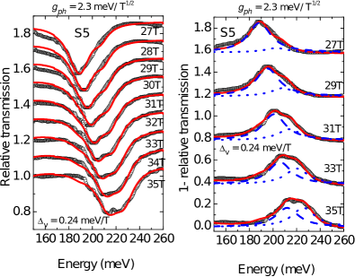
Figure 1: (color online). Left panel: Evolution of the $E_{01}$ transition for different values of the magnetic field beyond 27 T. Experimental transmission data for sample S5 (open circles) is compared with calculated transmission spectra (red lines), for different values of magnetic field, using the proposed CDW model. Right panel: 1 - (relative transmission) measured in the experiment and calculated (red lines) for the CDW phase, for magnetic fields $B$ = 27, 29, 31, 33, 35 T. Deconvolution of the experimental spectra into two Lorentzians is shown in blue dashed and dotted lines.

In Sec. II, we discuss these experimental observations and methods in more detail. We first interpret our experimental findings within a simplified model for valley symmetry breaking in Sec. III before deriving a more complete Hamiltonian in Sec. IV and calculating the optical conductivity in various broken symmetry phases in Sec. V. Finally, a comparison between experiment and theory is presented in Sec. VI, followed by conclusions in Sec. VII.

II Experimental observations and methods

In our experiment, precise infra-red transmission measurements were performed on multi-layer epitaxial graphene samples, at 1.8 K, under magnetic fields up to 35 T. The light (provided and analyzed by a Fourier transform spectrometer) was delivered to the sample by means of light-pipe optics. All experiments were performed with nonpolarized light, in the Faraday geometry with the wave vector of the incoming light parallel to the magnetic field direction and perpendicular to the plane of the samples. A Si bolometer was placed directly beneath the sample to detect the transmitted radiation. The response of this bolometer is strongly dependent on the magnetic field. Therefore, in order to measure the absolute transmission TA ($B,\omega)$, we used a sample-rotating holder and measure for each value of $B$ a reference spectrum through a hole. These spectra are normalized in turn with respect to TA($0,\omega$) to obtain a relative transmission spectrum TR($B,\omega$) which only displays the magnetic field dependent features. Those spectra are presented in Fig. 2.

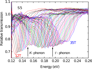
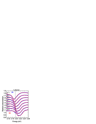
Figure 2: (color online). Top: Relative transmission spectra of sample S5, for different magnetic field values up to 35 T. Bottom: Evolution of the $E_{01}$ transition for different values of the magnetic field between 27 T and 34 T, for samples S4 (open dots) and S5 (full lines).

The samples were grown Berger on the C-terminated surface of SiC and display the characteristic transmission spectra of isolated graphene monolayers that arise from rotational stacking of the sheets Hass . The thickness $d$ of the SiC substrate has to be reduced significantly in order to minimize the very strong double-phonon absorption of SiC in the energy range of interest. In the first series $d$ was reduced to  $60\mu m$ and related samples have been used to perform the experiments reported earlier Orlita . One of them, named S4, was used to compare the data with those obtained on sample S5 from a new series where the thickness $d$ was further reduced down to  $32\mu m$. We compare in Fig. 2 the transmission spectra, at high fields, for samples S4 and S5. Technically speaking, the optical response of both samples is almost the same, showing that they have a similar number of active layers.

Taking into account all layer dielectric properties of each sample in a multi-layer dielectric model, we determine the effective number, $N_{eff}$, of graphene sheets with their respective carrier density (see Appendix). For samples S4 and S5, we have found that $N_{eff}=7$ with carrier densities $\{5.5,3.2,1.8,1.1,0.5,0.1,0.1\}10^{12}\textrm{cm}^{-2}$ and $\{6.0,3.5,2.0,1.2,0.5,0.1,0.1\}10^{12}\textrm{cm}^{-2}$ respectively. These carrier densities are fixed for each sample.

The transmission spectra of sample S5 at high magnetic fields are displayed in Fig. 1. We observe a new transition occurring at an energy higher than that of the CR line, growing in intensity when increasing the magnetic field. This behavior cannot be explained without breaking the SU(4) symmetry in graphene. In order to characterize more clearly these findings, one can treat the data, as a first step and in a very rough way, extracting from the transmission data the real part of the effective diagonal component of the conductivity $\sigma_{xx}(\omega,B)$ Sadowski . We have deconvoluted this result with two Lorentzians of equal width, extracting the evolution of the two extrema with the magnetic field. The resulting energies are displayed in Fig. 3 (top panel) for samples S4 and S5.

Though the procedure adopted at this initial level is quite rough, it provides important information: (i) The evolution of the lower energy line varies at low fields like $B^{1/2}$ (function F2($B$) in Fig. 3) with a coefficient proportional to the Fermi velocity $v_{F}$ and ends at higher fields with a similar dependence (function F1($B$)) but with a smaller value of $v_{F}$ which is, by itself, a sign of some interaction occurring at an energy close to that of the $\Gamma$-phonon; (ii) The second component of the deconvolution always appears at energies larger than that of the $\Gamma$-phonon; (iii) In principle, in the SU(4) symmetric picture, it is not possible to explain the occurrence of an additional transition, growing in intensity with $B$, at higher energies than the main transition line; (iv) It is therefore clear that the $\Gamma$-phonon plays a crucial role though it should not, indicative that the SU(4) symmetry is broken. Using these observations, we now have some guidelines to develop a theory which can explain quantitatively the experimental observations. In addition, we note that results for samples S4 and S5 are quite similar within the experimental errors. Knowing that the active layers which contribute to the $E_{01}$ transition should have a filling factor $\nu\leq 2$ ( $\nu=N_{s}\Phi_{0}/B,\Phi_{0}$ being the flux quantum and $N_{s}$ the carrier density) and that, in samples S4 and S5, the carrier density for active layers do not have the same sequence, the physical mechanisms describing the experimental findings should not be very dependent on the doping of active layers. This is indeed the case as discussed below.

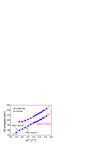
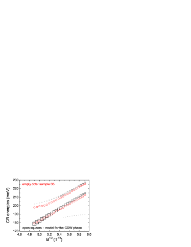
Figure 3: (color online). Top: CR energies, resulting from the deconvolution of the experimental transmission traces, as a function of $\sqrt{B}$ for samples S4 (full dots) and S5 (open dots). Error bars are similar for both samples. The full lines are a linear fit of the data for the low energy transition at low (F2($B$)) and high (F1($B$)) field. Bottom: Comparison of the variation of experimental CR energies for sample S5 (open dots), with that calculated for the CDW phase (open squares), as a function of $\sqrt{B}$. The size of the open squares mimics the relative oscillator strength of the optical transition.

III Simplified model for valley symmetry breaking

To illustrate how the electron-phonon interaction and the valley symmetry breaking give rise to the observed features in the transmission spectrum, we first introduce a simplified model for the interaction of the $\Gamma$ phonon with the $E_{01}$ excitation, before discussing the full SU(4) calculation. The simplified model provides a minimal description of the valley symmetry breaking by neglecting the spin degree of freedom in the $n=0$ LL. We assume that $K$ and $K^{\prime}$ sublevels of the $n=0$ LL are separated in energy by $\Delta_{V}$, and have different filling factors $\nu_{K}$ and $\nu_{K^{\prime}}$. Considering just the $n=0$ to $n=1$ transitions, the interaction with the $\Gamma$ phonon is captured by the Hamiltonian (in the basis of creating an electronic excitation in $K$, electronic excitation in $K^{\prime}$, and a $\Gamma$ phonon, in that order)

$$H=\begin{pmatrix}E_{01}-\Delta_{V}/2&0&g_{ph}\sqrt{\nu_{K}}\\ 0&E_{01}+\Delta_{V}/2&-g_{ph}\sqrt{\nu_{K^{\prime}}}\\ g_{ph}\sqrt{\nu_{K}}&-g_{ph}\sqrt{\nu_{K^{\prime}}}&\hbar\omega_{\Gamma}\end{pmatrix}.$$ (1)

where $g_{ph}$ characterizes the electron-$\Gamma$-phonon interaction. The optical conductivity is calculated using the Green’s function formalism introduced by Toyozawa Toyozawa1 . The diagonal component of the conductivity is:

$$\sigma_{xx}(\hbar\omega)=\frac{1}{\omega}\textrm{Im}M^{\dagger}_{x}G(\hbar\omega)M_{x}$$ (2)

where the Green’s function is $G=\left(\hbar\omega-H-i\eta\right)^{-1}$, with $\eta\rightarrow 0^{+}$ (see Sec. IV.2). The optical matrix elements for the simplified model are $M_{x}^{\dagger}=\left(\sqrt{\nu_{K}},\sqrt{\nu_{K^{\prime}}},0\right)$. The simplified model explains the splitting of the main transition line in the two limits $E_{01}\approx\hbar\omega_{\Gamma}$ and $E_{01}\gg\hbar\omega_{\Gamma}$. In the absence of valley splitting ($\Delta_{V}=0$ and $\nu_{K}=\nu_{K^{\prime}}$), the eigenstates of the pure electronic part of $H$ in Eq. 1 are valley-symmetric and valley-antisymmetric combinations of $E_{01}$ transitions, i.e. $\frac{1}{2}\left(c^{\dagger}_{1,K}c_{0,K}+c^{\dagger}_{1,K^{\prime}}c_{0,K^{\prime}}\right)\lvert\textrm{GS}\rangle$ and $\frac{1}{2}\left(c^{\dagger}_{1,K}c_{0,K}-c^{\dagger}_{1,K^{\prime}}c_{0,K^{\prime}}\right)\lvert\textrm{GS}\rangle$, respectively, where $\rvert{}\textrm{GS}\rangle$ denotes the ground state and $c^{\dagger}_{n,K}$ are creation operators at LL $n$ and valley $K$. The valley-symmetric combination is infra-red active but does not interact with the $\Gamma$ phonon, while the valley-antisymmetric combination is infra-red inactive and interacts with the $\Gamma$ phonon. The symmetry breaking valley splitting term $\Delta_{V}$ allows both eigenmodes to interact with the $\Gamma$ phonon while remaining infra-red active, inducing a splitting of the main transmission line in the vicinity of the $\Gamma$ phonon frequency. Away from the $\Gamma$ phonon frequency ($E_{01}\gg\hbar\omega_{\Gamma}$), $E_{01}$ transitions at $K$ and $K^{\prime}$ interact weakly with the phonon and the splitting of the main transmission line is controlled directly by the energy difference $\Delta_{V}$.

IV Theory of magneto-phonon resonance in the presence of SU(4) symmetry breaking

We reintroduce the spin degree of freedom and the $n=-1$ to $n=0$ transitions in order to obtain a quantitative understanding of the experiment. We consider different theoretical models of the $n=0$ LL SU(4) symmetry breaking, taking into account the effects of $\nu\neq 0$ and disorder by introducing Gaussian broadening into a mean field theory (Sec. IV.1). Different symmetry-breaking phases are represented in the mean field theory by different orderings and filling factors of the four sublevels of the $n=0$ LL. We consider four candidate symmetry-breaking phases that have been proposed in the literature Kharitonov : Ferromagnetic(F), Charge Density Wave (CDW), Canted Antiferromagnetic (CAF) and Kekulé-distortion (KD), and calculate the optical conductivity using Eq. 2 with the appropriate Hamiltonian $H$ for each phase. Treating these phases on the same footing (detailed in Sec. V), we find that each phase results in characteristic features in the evolution of the transmission spectrum as a function of the magnetic field. By examining the intensities and positions of the transmission lines, we identify the symmetry broken phase in the samples used in our experiment as the CDW type Fuchs ; Jung .

IV.1 Description of the ground state

We assume that the ground state is a single Slater determinant of the form:

$$|GS\rangle=\prod_{j=1}^{4}\prod_{m_{j}=1}^{N_{j}}\Psi_{j,m_{j}}^{\dagger}|0\rangle$$ (3)

the index j runs over the 4-dimensional spin/valley space and $m_{j}$ describe the ”guiding center” degree of freedom. The state ($j,m_{j}$) is represented by the wavefunction $\xi_{j}\phi_{m_{j}}(\overrightarrow{r})$ where $\xi_{j}$ is a four-component spinor and $\phi_{m_{j}}(\overrightarrow{r})$ is the orbital part of the wavefunction. These wavefunctions belong to the $n=0$ landau level (LL) of graphene. The occupation numbers $N_{j}$ count the number of $j$ states that are occupied in this ground state.

There are different models proposed to describe the symmetry-broken phase of graphene which have been reviewed by Kharitonov Kharitonov . For a given model, we assume that the system is polarized along a certain direction in $j$-space. For instance, with increasing order of energies, $j=1,2,3,4$ corresponds to ($K^{\prime}\uparrow,K^{\prime}\downarrow,K\uparrow,K\downarrow$) in the charge density wave (CDW) phase. The remaining degrees of freedom, $\phi_{m_{j}}(\overrightarrow{r})$ and $N_{j}$, are treated as variational parameters, subject to the constraint $N_{1}+N_{2}+N_{3}+N_{4}=N$. We minimize the energy of the ground state $E_{GS}=\langle GS|H_{0}+H_{e-e}+H_{disorder}|GS\rangle$. Here $H_{0}$ is the single part of the Hamiltonian without disorder, $H_{e-e}$ the interaction term and $H_{disorder}$ the disorder potential. Because we assume a single Slater determinant, we can apply mean-field theory and obtain single-particle energy levels $E_{j,m_{j}}$ (The origin of the energies is taken to be at the energy of the $n=0$ LL of the non-interacting system).

In a system with finite disorder, the energy levels $E_{j,m_{j}}$ are clustered about mean values $E_{j}=\underset{m_{j}}{\textrm{avg }}E_{j,m_{j}}$. We remove the $m_{j}$ degrees of freedom by replacing the energy levels $E_{j,m_{j}}$ by broadened energy levels centered at $E_{j}$. There is a Fermi level $E_{F}$ which fixes the occupation numbers $N_{j}$ when the graphene layer is doped with a total filling factor $\nu$. Assuming the broadening to be of Gaussian type with a width $\gamma_{0}$ the Fermi level is determined by solving the following equation:

$$\nu=\sum_{j}\textrm{Erf}(\frac{E_{F}-E_{j}}{\sqrt{2}\gamma_{0}})$$ (4)

from which one can calculate the individual filling factors $\nu_{j}=(1+\textrm{Erf}(\frac{E_{F}-E_{j}}{\sqrt{2}\gamma_{0}}))/2$ for each level $E_{j}$. These $E_{j}$ will be used, later on, as fitting parameters dependent on the broken-symmetry phase under consideration. Note that in this approach all optical transitions to or from the $n=0$ LL are allowed.

IV.2 Description of the optical transitions

We first consider the transitions from the $n=0$ LL to $n=1$ LL. The Hamiltonian of the magneto-excitons, including their interaction with the $\Gamma$-phonon, denoted $H_{\circlearrowright}$ (reminding that it describes the optical transitions allowed in the $\sigma^{+}$ polarization), is:

$$H_{\circlearrowright}=\begin{pmatrix}\hbar\omega_{01}-E_{1}&0&0&0&g_{1}\sqrt{\nu_{1}}\\ 0&\hbar\omega_{01}-E_{2}&0&0&g_{2}\sqrt{\nu_{2}}\\ 0&0&\hbar\omega_{01}-E_{3}&0&g_{3}\sqrt{\nu_{3}}\\ 0&0&0&\hbar\omega_{01}-E_{4}&g_{4}\sqrt{\nu_{4}}\\ g_{1}^{*}\sqrt{\nu_{1}}&g_{2}^{*}\sqrt{\nu_{2}}&g_{3}^{*}\sqrt{\nu_{3}}&g_{4}^{*}\sqrt{\nu_{4}}&\hbar\omega_{ph}\\ \end{pmatrix}.$$ (5)

where $\hbar\omega_{01}$ is the energy of the $E_{01}$ transition from the $n=0$ LL to $n=1$ LL in the absence of interactions and $\hbar\omega_{ph}$ that of the $\Gamma$-phonon. This Hamiltonian describes the excitations from the 4 sublevels $\{E_{j},j=1..4\}$ of the $n=0$ LL to the $n=1$ LL. The matrix elements $\{g_{j},j=1..4\}$ respectively describe their interaction with the $\Gamma$-phonon, and is dependent on the wavefunction character of the 4 sublevels (i.e., dependent on the broken-symmetry phase). In general, $g_{j}\propto\sqrt{B}$ Goerbig , with a prefactor dependent on $j$ and the broken-symmetry phase.

Similarly, the Hamiltonian describing the magneto-excitons for the transitions from the $n=-1$ LL to the $n=0$ LL (allowed in the $\sigma^{-}$ polarization) is written as:

$$H_{\circlearrowleft}=\begin{pmatrix}\hbar\omega_{01}+E_{1}&0&0&0&g_{1}\sqrt{1-\nu_{1}}\\ 0&\hbar\omega_{01}+E_{2}&0&0&g_{2}\sqrt{1-\nu_{2}}\\ 0&0&\hbar\omega_{01}+E_{3}&0&g_{3}\sqrt{1-\nu_{3}}\\ 0&0&0&\hbar\omega_{01}+E_{4}&g_{4}\sqrt{1-\nu_{4}}\\ g_{1}^{*}\sqrt{1-\nu_{1}}&g_{2}^{*}\sqrt{1-\nu_{2}}&g_{3}^{*}\sqrt{1-\nu_{3}}&g_{4}^{*}\sqrt{1-\nu_{4}}&\hbar\omega_{ph}\\ \end{pmatrix}.$$ (6)

The total Hamiltonian $H$ describing the magneto-excitons is therefore:

$$H=\begin{pmatrix}H_{\circlearrowright}&0\\ 0&H_{\circlearrowleft}\\ \end{pmatrix}.$$ (7)

We will also need to introduce the optical matrix elements $M_{x}$ and $M_{y}$ for corresponding transitions. These matrix elements depend on the ground state under consideration. In CDW case they are (see Sec. V.1) : $M_{x}/v_{0}=\{\sqrt{\nu_{1}}$, $\sqrt{\nu_{2}}$, $\sqrt{\nu_{3}}$, $\sqrt{\nu_{4}}$, 0, $-\sqrt{1-\nu_{1}}$, $-\sqrt{1-\nu_{2}}$, $-\sqrt{1-\nu_{3}}$, $-\sqrt{1-\nu_{4}}$, $0\}$ and $M_{y}=iM_{x}$. For a different scenario, the optical matrix elements will be transformed to a different basis, as will be detailed in Sec. V.

The Green’s function for the magneto-excitons, is obtained as $G=((\hbar\omega+i\gamma_{01}).\text{I}-H)^{-1}$ (where I is the unit matrix and $\gamma_{01}$ the broadening of the $E_{01}$ transition). This allows us to calculate the different components of the conductivity:

$$\sigma_{xx}(\omega)=\frac{i}{\omega}M_{x}^{T}.G.M_{x}$$ (8)

$$\sigma_{xy}(\omega)=\frac{1}{\omega}M_{x}^{T}.G.M_{y}^{*}$$

V Optical conductivity in the different phases

Here, we calculate the optical conductivity for the different symmetry broken phases, using Eq. 8.

V.1 Charge density wave (CDW) phase

The CDW phase is characterized, at filling factor $\nu=0$, by two electronic LL full in one valley (say $K^{\prime}$ for instance) and two LL empty in the other valley ($K$). We will introduce a valley asymmetry $\Delta_{V}$ mainly determined by electron-electron interactions Kharitonov and a Zeeman splitting $\Delta_{S}$. Therefore the sequence of sublevels take the following form:

$$E_{1}(K^{\prime}\uparrow) =-\Delta_{V}/2-\Delta_{S}/2$$ (9)

$$E_{2}(K^{\prime}\downarrow) =-\Delta_{V}/2+\Delta_{S}/2$$

$$E_{3}(K\uparrow) =\Delta_{V}/2-\Delta_{S}/2$$

$$E_{4}(K\downarrow) =\Delta_{V}/2+\Delta_{S}/2$$

In this case, the parameters governing the electron-$\Gamma$phonon interaction $g_{1}$, $g_{2}$ on one hand and $g_{3}$, $g_{4}$ on the other hand are of opposite sign. That is,

$$\langle GS_{CDW}+\Gamma\textrm{phonon}\rvert H_{e-ph}\Psi^{\dagger}_{Ks,1}\Psi_{Ks,0}\lvert GS_{CDW}\rangle =g_{ph}/\sqrt{2}$$ (10)

$$\langle GS_{CDW}+\Gamma\textrm{phonon}\rvert H_{e-ph}\Psi^{\dagger}_{K^{\prime}s,1}\Psi_{K^{\prime}s,0}\lvert GS_{CDW}\rangle =-g_{ph}/\sqrt{2}$$

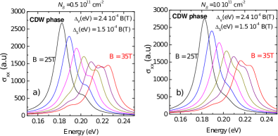
Figure 4: (color online). CDW phase with $\Delta_{V}\propto B$: evolution of the $\sigma_{xx}$ component of the conductivity for different values of the magnetic field between 25 T and 35 T for a) a carrier density $N_{s}=0.5\times 10^{11}\text{cm}^{-2}$ and b) $N_{s}=1\times 10^{12}\text{cm}^{-2}$. In both cases $g_{ph}=2.3\times\sqrt{B[T]}$ meV.

where $\Psi^{\dagger}_{K,s,n}$ is the creation operator for electrons in valley $K$, spin $s$, Landau level $n$. On the other hand, the electron-light interaction (which determines $M$) has the same sign at both valleys.

$$\langle GS_{CDW}+\textrm{photon}\rvert H_{e-light}\Psi^{\dagger}_{Ks,1}\Psi_{Ks,0}\lvert GS_{CDW}\rangle =1$$ (11)

$$\langle GS_{CDW}+\textrm{photon}\rvert H_{e-light}\Psi^{\dagger}_{K^{\prime}s,1}\Psi_{K^{\prime}s,0}\lvert GS_{CDW}\rangle =1$$

The results obtained for this phase are presented in Fig. 4, assuming $\Delta_{V}$ proportional to $B$, for two extreme values of the carrier density. The electron-phonon coupling was taken to be $g_{ph}=2.3\times\sqrt{B[T]}$ meV, which agrees with density functional theory (DFT) calculations Piscanec and experiments Lazzeri ; Yan ; Pisana . The results are not very dependent on $N_{s}$. The value of $\Delta_{S}=0.15$ meV $B$ corresponds to a g-factor of 2.6 to be compared with $2.7\pm 0.2$ reported in Kurganova . The splitting of the transition is directly governed by the amplitude of $\Delta_{V}$ whereas the introduction of $\Delta_{S}$ modifies only the relative amplitude of the two transitions. In all cases both $\Delta_{V}$ and $g_{ph}$ need to be finite to observe the effect. We finally note that, in this case, $\Delta_{V}>\Delta_{S}$ in coherence with the assumption made in our previous work Orlita .

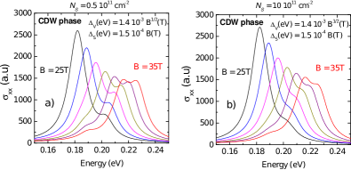
Figure 5: (color online). CDW phase with $\Delta_{V}\propto\sqrt{B}$: evolution of the $\sigma_{xx}$ component of the conductivity for different values of the magnetic field between 25 T and 35 T for a) a carrier density $N_{s}=0.5\times 10^{11}\text{cm}^{-2}$ and b) $N_{s}=1\times 10^{12}\text{cm}^{-2}$. In both cases $g_{ph}=2.3\times\sqrt{B[T]}$ meV.

However there is no clear consensus about the field dependence on $\Delta_{V}$ Kharitonov . Therefore one can alternatively assume that $\Delta_{V}$ is proportional to $\sqrt{B}$. The corresponding results are displayed in Fig. 5 keeping all other parameters fixed. We obtained essentially the same results as in Fig. 4. Within the experimental errors we will not be able to differentiate between the two magnetic field variations of $\Delta_{V}$.

The CDW state is compatible with the experimental results as we will see below.

V.2 Kekulé-distortion (KD) phase

In this phase Kharitonov , the $K$ and $K^{\prime}$ valleys hybridize into linear combinations $\overline{K}$, $\overline{K^{\prime}}$. At $\nu=0$, both spin $\uparrow$ and spin $\downarrow$ electrons occupy one of these valley-combinations, say $\overline{K}$. The $\nu=0$ ground state for the KD phase is $\Psi_{\overline{K}\uparrow,0}^{\dagger}\Psi_{\overline{K}\downarrow,0}^{\dagger}|0\rangle$. Therefore, the ”natural” basis for this phase, where the density matrix is diagonal, is $\{\overline{K}\uparrow,\overline{K}\downarrow,\overline{K^{\prime}}\uparrow,\overline{K^{\prime}}\downarrow\}$ in contrast to the basis $\{K\uparrow,K\downarrow,K^{\prime}\uparrow,K^{\prime}\downarrow\}$ used in the CDW phase. Therefore the sequence of sublevels take the following form:

$$j=1 :\overline{K}\uparrow$$ (12)

$$j=2 :\overline{K}\downarrow$$

$$j=3 :\overline{K^{\prime}}\uparrow$$

$$j=4 :\overline{K^{\prime}}\downarrow$$

The transformation rules for the operators in this basis are

$$\Psi_{\overline{K},s,n}^{\dagger}= \frac{1}{\sqrt{2}}\left(\Psi_{K,s,n}^{\dagger}+e^{i\phi}\Psi_{K^{\prime},s,n}^{\dagger}\right)$$ (13)

$$\Psi_{\overline{K^{\prime}},s,n}^{\dagger}= \frac{1}{\sqrt{2}}\left(\Psi_{K,s,n}^{\dagger}-e^{i\phi}\Psi_{K^{\prime},s,n}^{\dagger}\right)$$

where $\Psi^{\dagger}_{\overline{K},s,n}$ is the creation operator for electrons in valley state $\overline{K}$, spin $s$, Landau level $n$. Making use of this change of basis (Eq. 13) and Eq. 10 and Eq. 11, we derive that the electron-light matrix elements do not change with respect to the CDW phase, and the electron-phonon matrix elements $g$ vanish by symmetry. That is,

$$\langle GS_{KD}+\Gamma\textrm{phonon}\rvert H_{e-ph}\Psi^{\dagger}_{\overline{K}\uparrow,1}\Psi_{\overline{K}\uparrow,0}\lvert GS_{KD}\rangle =0$$ (14)

$$\langle GS_{KD}+\textrm{photon}\rvert H_{e-light}\Psi^{\dagger}_{\overline{K}\uparrow,1}\Psi_{\overline{K}\uparrow,0}\lvert GS_{KD}\rangle =1$$

and the same for $\overline{K^{\prime}}$. The structure of the Hamiltonian (Eq.7) becomes only diagonal and no splitting is observed when calculating the conductivity. Therefore the KD phase does not explain the experimental results.

V.3 Ferromagnetic (F) phase

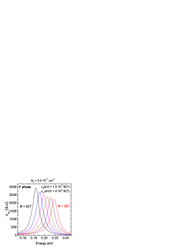
Figure 6: (color online). Ferromagnetic phase with $\Delta_{V}\propto B$: evolution of the $\sigma_{xx}$ component of the conductivity for different values of the magnetic field between 25 T and 35 T for a carrier density $N_{s}=5.0\times 10^{11}\text{cm}^{-2}$ and $g_{ph}=2.3$ meV/$\text{T}^{1/2}$.

In the F phase Kharitonov , the ground state, at filling factor $\nu=0$, is composed in both valleys $K$ and $K^{\prime}$ of a single full LL with the same spin. In analogy with the CDW phase, we will introduce a valley asymmetry $\Delta_{V}$ and a Zeeman splitting $\Delta_{S}$. Therefore the sequence of energy levels take the following form:

$$E_{1}(K^{\prime}\downarrow) =-\Delta_{V}/2-\Delta_{S}/2$$ (15)

$$E_{2}(K\downarrow) =\Delta_{V}/2-\Delta_{S}/2$$

$$E_{3}(K^{\prime}\uparrow) =-\Delta_{V}/2+\Delta_{S}/2$$

$$E_{4}(K\uparrow) =\Delta_{V}/2+\Delta_{S}/2$$

Note that, in this case, $\Delta_{S}$ should be larger than $\Delta_{V}$ to preserve the ferromagnetic nature of the state. In the present case the parameters governing the electron-$\Gamma$phonon interaction (Eq.5,6) $g_{1}$, $g_{3}$ on one hand and $g_{2}$, $g_{4}$ in the other hand are of opposite sign.

The results are displayed in Fig. 6 where we have taken for $\Delta_{S}$ the same evolution that in the CDW phase and $\Delta_{V}\propto B$. The conductivity does not show any significant splitting of the main line. In fact there is an eigenvalue of the corresponding Hamiltonian larger than that of the main line but it remains optically inactive. Therefore here also, the F phase does not explain the experimental results.

V.4 Canted anti-ferromagnetic (CAF) phase

The CAF phase for the ground state is described by a spin in direction $\theta_{K}$ in valley $K$ and a spin in direction $\theta_{K^{\prime}}$ in valley $K^{\prime}$. (The directions $\theta_{K}$ and $\theta_{K^{\prime}}$ are in general not opposite to each other except in the special case of the anti-ferromagnetic phase). The direction $\theta_{K}$ is oriented at an angle $\theta$ relative to the magnetic field $B$ and the direction $\theta_{K^{\prime}}$ at an angle $-\theta$ with respect to it. (In the anti-ferromagnetic phase, $\theta=\pi/2$). Here the Zeeman splitting should vary like $\Delta_{S}\propto\cos\theta$ and if $\theta$ is close to $\pi/2$ this term should not play a dominant role. We choose the following order of states:

$$E_{1}(K,\theta_{K}) =-\Delta_{1}/2-\Delta_{2}/2$$ (16)

$$E_{2}(K^{\prime},\theta_{K^{\prime}}) =-\Delta_{1}/2+\Delta_{2}/2$$

$$E_{3}(K,\pi+\theta_{K}) =\Delta_{1}/2-\Delta_{2}/2$$

$$E_{4}(K^{\prime},\pi+\theta_{K^{\prime}}) =\Delta_{1}/2+\Delta_{2}/2$$

where the introduction of $\Delta_{1}$ reflects the CAF pattern of spin. We assume in addition that the asymmetry between valleys is reflected by $\Delta_{2}$ (favoring here the $K$ valley). To preserve the CAF phase $\Delta_{2}$ should be smaller than $\Delta_{1}$. Similar to the F phase, the parameters governing the electron-$\Gamma$phonon interaction (Eq.5,6) $g_{1}$, $g_{3}$ on one hand and $g_{2}$, $g_{4}$ in the other hand are of opposite sign.

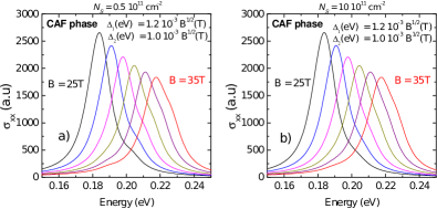
Figure 7: (color online). CAF phase with $\Delta_{1}\propto\sqrt{B}$ and $\Delta_{2}\propto\sqrt{B}$: evolution of the $\sigma_{xx}$ component of the conductivity for different values of the magnetic field between 25 T and 35 T for a) a carrier density $N_{s}=0.5\times 10^{11}\text{cm}^{-2}$ and b) $N_{s}=1\times 10^{12}\text{cm}^{-2}$. In both cases $g_{ph}=2.3$ meV/$\text{T}^{1/2}$.

The results are displayed in Fig. 7 where we have taken, $\Delta_{1}$ and $\Delta_{2}$ proportional to $\sqrt{B}$. The results are not very dependent on the carrier concentration. We observe indeed a splitting of the transition when both $\Delta_{2}$ and $g_{ph}$ are different from zero : in fact the splitting is governed by $\Delta_{2}$. In the present case we do not have, a priori, a guide for choosing the values of $\Delta_{1}$ and $\Delta_{2}$. In order to be consistent with experimental results, we have taken for $\Delta_{1}$ a value which provides an upper transition energy close to that observed.

However the evolution of the spectra does not reflect the experimental observations: whatever is the choice of parameters, the intensity of the high energy transition never reaches that of the main transition in contrast to the CDW phase where it should become dominant at fields higher than 35 T. This is discussed further in the next section.

VI Comparison of experiment and theory

The KD, F and CAF phases result in transmission spectra incompatible with experiment (Fig. 8). In the KD phase, electrons occupy linear combinations of the $K$ and $K^{\prime}$ valleys; the electron-phonon matrix elements vanish by symmetry, resulting in a single transmission line. For the F phase, the occupancy of the $K$ and $K^{\prime}$ valleys are almost equal (Sec. V.3), and there is no significant splitting of the main transmission line (Fig. 8) . Similarly, the calculated transmission spectra for the CAF phase show a second CR line of much lower intensity than the main CR line. Deconvoluting these spectra with two Lorentzians we find a ratio of the CR weights of $0.9\pm 0.05$ for the experiment, to be compared to the value 0.9 for the CDW phase and 0.4 for the CAF phase. Despite the introduction of valley asymmetry into the CAF phase, we find that it cannot explain the observed evolution of CR energies in the experiment.

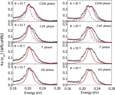
Figure 8: (color online). Real part of the conductivity measured in the experiment (open dots) and calculated with the CDW, CAF, F and KD phases (red continuous lines), for magnetic fields $B=31T$ (left panel) and $35T$ (right panel). The Deconvolution of the model into two Lorentzians is shown for the CDW and CAF phases (blue dashed and dotted lines).

The CDW phase has unequal occupation numbers of the $n=0$ LL at the $K$ and $K^{\prime}$ valleys, corresponding to a density modulation of the graphene $A$ and $B$ sublattices in real space. Unlike the ideal disorder-free CDW discussed in Kharitonov , both $K$ and $K^{\prime}$ valleys have non-zero occupation number in our calculation, due to disorder-induced broadening. Nevertheless, the mechanism giving rise to the splitting of the $E_{01}$ transmission line remains essentially the same as illustrated by the simple model (Eq. 1) above.

The spin and valley splittings $\Delta_{S}$ and $\Delta_{V}$ parameterize our model for the CDW phase and determine the filling factors that enter the Hamiltonian and the optical matrix elements. We fix $\Delta_{S}$ using the experimental graphene g-factor measured in Ref.Kurganova . We treat $\Delta_{V}$ as a fitting parameter, obtaining $\Delta_{V}=0.24\times B[\textrm{T}]\textrm{meV}$. In our calculations, we use $g_{ph}=2.3\times\sqrt{B[\textrm{T}]}\textrm{meV}$, which is in good agreement with density functional theory (DFT) calculations Piscanec and experiments Lazzeri ; Yan ; Pisana . We take the position of the $E_{01}$ transition line and its broadening to be given by $v_{F}=1.01\times 10^{6}\textrm{ms}^{-1}$ and $\gamma_{01}[\textrm{meV}]=3+0.8\sqrt{B[\textrm{T}]}$ respectively, consistent with their measured values at low magnetic fields away from the $\Gamma$-phonon frequency. For the parameter $\gamma_{0}$ characterizing the broadening of the Landau levels in Eq.4, we have taken $\gamma_{0}=\gamma_{01}/2$ because the broadening of the $E_{01}$ transition should have contributions from both the $n=0$ and $n=1$ Landau levels. The calculations for the splitting at high magnetic fields are in excellent agreement with the experimental transmission spectra for both samples S4 (Fig. 9) and S5 (Fig. 1). We neglect $K$-phonon absorption Orlita , which might account for the discrepancy between theory and experiment at the lower frequency and magnetic field range of our data.

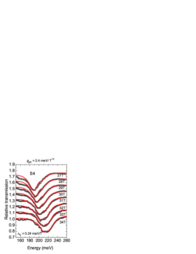
Figure 9: (color online). Fit of the experimental data (open dots) for sample S4 with the conductivity model derived for the CDW phase (continuous lines) using $\Delta_{V}=0.24$ meV/T and $g_{ph}=2.4$ meV/$\text{T}^{1/2}$.

Upon changing the carrier density $N_{s}$ by a factor of $\sim 10$ in our calculations, we find only minor changes in the transmission spectra, which is consistent with the observation that samples S4 and S5 have remarkably similar transmission spectra despite having different carrier densities. This is because the disorder induced broadening reduces the dependence of the sublevel filling factors ($\nu_{K\uparrow}$, etc.) on the carrier density.

For symmetry breaking driven by electron-electron interactions, the details of the screening function plays a vital role in determining the nature of the ground state. The additional screening afforded by the multiple graphene layers in our epitaxial graphene samples might favor the CDW configuration, with two electrons on the same sublattice, over the CAF state observed in hBN-supported samples Young2 . Furthermore, coupling between rotationally misaligned layers breaks the local A-B sublattice (i.e. valley) symmetry He1 ; He2 , promoting the CDW ground state.

VII Conclusions

In conclusion, we have used magneto-optical spectroscopy to characterize a SU(4) symmetry broken phase in our epitaxial graphene samples. Based on the evolution of the transmission lines near the $\Gamma$ phonon frequency, we identify this phase as a CDW phase for the specific samples considered, with different occupation numbers at valleys $K$ and $K^{\prime}$. Because of the valley-sensitive nature of the electron-phonon interaction, the transmission study used here complements spin-sensitive transport measurements in tilted magnetic fields in the study of symmetry breaking in graphene. Our experimental method can be applied to open questions such as symmetry breaking of the different LLs in graphene and bilayer graphene, as well as the effect of disorder on the broken symmetry phase in these systems.

Appendix

In general, the detailed analysis of magneto-transmission spectra requires the use of a multi-layer dielectric model including all layer dielectric properties of the sample. In particular, for each graphene sheet, one has to introduce the corresponding components of the optical conductivity tensor $\sigma_{xx}(\omega)$ and $\sigma_{xy}(\omega)$. Here, the $x$ and $y$-axis lie in the plane of the sample. For instance $\sigma_{xx}(\omega)$, in a one-electron approximation, for transitions involving the $n=0$ LL, is written as:

$$\sigma_{xx}(\omega,B)=i\frac{e^{3}B}{h\omega}\sum_{r,s}\frac{M^{2}_{r,s}(f_{r}(B)-f_{s}(B))}{\hbar\omega-E_{r,s}(B)+i\Gamma_{rs}(B)}$$ (17)

where $r$,$s$ scan the values 0 and $\pm 1$, $0\leq f_{r}\leq 1$ is the occupation factor of the LL $r$, $M_{r,s}$ the optical matrix element, $E_{r,s}=E_{r}-E_{s}=E_{01}$ and $\Gamma_{rs}(B)=\gamma_{01}(B)$ measures the broadening of the transition. $M_{r,s}\propto v_{0}$ where $v_{0}$ is the Fermi velocity given by LDA calculations Bychkov . In the present work, we have taken for all samples $v_{0}=0.85\times 10^{6}ms^{-1}$. This is a different parameter from $v_{F}$ which appears in $E_{01}$ because the energies and wavefunctions are corrected to different extents by the electron-electron interaction Bychkov . This approach requires the knowledge of the number of effective active layers as well as their carrier densities $N_{s}$ ($\nu=N_{s}\Phi_{0}/B$, $\Phi_{0}$ being the flux quantum) which, in turn, implies some approximations.

The multi-layer dielectric model assumes that each graphene sheet is uniformly spread over the sample. This is a strong assumption, difficult to justify a priori and we have been lead to correct it by assuming a mean coverage which, in the present case for samples S4 and S5, has been determined to be about 70 per cent. We next evaluate the number $N_{eff}$ for each sample. In the range of magnetic fields 12 to 17 T, the relative transmission spectra (Fig. 2, top panel) reaches values above 1 which depends on the number $N_{eff}$: we have therefore a guide to estimate this quantity. We estimate $N_{eff}=7$ for samples S4 and S5.

The carrier density $N_{s}$ for each layer is determined in the following way: one knows that, for $2<\nu<6$, upon increasing $B$, the intensity of the $E_{01}$ absorption starts to increase, at the expense of the intensity of the $E_{12}$ transition ($E_{12}=E_{2}-E_{1}$). The intensity does not change with $B$ for $\nu<2$. Therefore, the disappearance of the optical transition $E_{12}$ corresponds to $\nu=2$. Following the transmission spectra as a function of $B$, one can evaluate the carrier density $N_{sm}$ for each layer $m$. This is an iterative process which converges reasonably (within 20 per cent) but has to be done independently for each sample. The value of $N_{s1}$ for the layer close to the SiC substrate can be set arbitrary to 5 to 6 $10^{12}cm^{-2}$ as given by transport data on samples grown under similar conditions: this layer indeed and the two following ones do not contribute to the transition $E_{01}$ in the present experiment. Finally, in the range of magnetic field larger than 27 T, where we focus our attention in this paper, the number of optically active layers (for optical transitions involving the $n=0$ LL) ranges between 3 to 4 for samples S4 and S5 with carrier densities ranging from 0.5 to 12 $\times 10^{11}\text{cm}^{-2}$.

References

- (1) Y. Zhang, Z. Jiang, J. P. Small, M. S. Purewal, Y.-W. Tan, M. Fazlollahi, J. D. Chudow, J. A. Jaszczak, H. L. Stormer, and P. Kim, Phys. Rev. Lett. 96, 136806 (2006).
- (2) Y. Zhao, P. Cadden-Zimansky, F. Ghahari, and P. Kim, Phys. Rev. Lett. 108, 106804 (2012).
- (3) Y. J. Song, A. F. Otte, Y. Kuk, Y. Hu, D. B. Torrance, P. N. First, W. A. de Heer, H. Min, S. Adam, M. D. Stiles, A. H. MacDonald, and J. A. Stroscio, Nature 467, 185-189 (2010).
- (4) D. L. Miller, K. D. Kubista, G. M. Rutter, M. Ruan, W. A. de Heer, M. Kindermann, P. N. First, and J. A. Stroscio, Nat Phys 6, 811-817 (2010).
- (5) A. F. Young, C. R. Dean, L. Wang, H. Ren, P. Cadden-Zimansky, K. Watanabe, T. Taniguchi, J. Hone, K. L. Shepard, and P. Kim, Nat Phys 8, 550-556 (2012).
- (6) A. F. Young, J. D. Sanchez-Yamagishi, B. Hunt, S. H. Choi, K. Watanabe, T. Taniguchi, R. C. Ashoori, and P. Jarillo-Herrero, Nature 505, 528-532 (2014).
- (7) G. L. Yu, R. Jalil, B. Belle, A. S. Mayorov, P. Blake, F. Schedin, S. V. Morozov, L. A. Ponomarenko, F. Chiappini, S. Wiedmann, U. Zeitler, M. I. Katsnelson, A. K. Geim, K. S. Novoselov, and D. C. Elias, PNAS 110, 3282-3286 (2013).
- (8) F. Amet, J. R. Williams, K. Watanabe, T. Taniguchi, and D. Goldhaber-Gordon, Phys. Rev. Lett. 112, 196601 (2014).
- (9) M. Kharitonov, Phys. Rev. B 85, 155439 (2012) and references therein.
- (10) D. A. Abanin, B. E. Feldman, A. Yacoby, and B. I. Halperin, Phys. Rev. B 88, 115407 (2013).
- (11) I. Sodemann and A. H. MacDonald, Phys. Rev. Lett. 112, 126804 (2014).
- (12) B. Roy, M. P. Kennett, and S. D. Sarma, arXiv:1406.5184 (2014).
- (13) E. A. Henriksen, P. Cadden-Zimansky, Z. Jiang, Z. Q. Li, L.-C. Tung, M. E. Schwartz, M. Takita, Y.-J. Wang, P. Kim, and H. L. Stormer, Phys. Rev. Lett. 104, 067404 (2010).
- (14) M. Orlita, L. Z. Tan, M. Potemski, M. Sprinkle, C. Berger, W. A. de Heer, S. G. Louie, and G. Martinez, Phys. Rev. Lett. 108, 247401 (2012).
- (15) C. H. Yang, F. M. Peeters, and W. Xu, Phys. Rev. B 82, 075401 (2010).
- (16) M. O. Goerbig, J.-N. Fuchs, K. Kechedzhi, and V. I. Fal’ko, Phys. Rev. Lett. 99, 087402 (2007).
- (17) C. Berger, Z. Song, T. Li, X. Li, A. Y. Ogbazghi, R. Feng, Z. Dai, A. N. Marchenkov, E. H. Conrad, P. N. First, and W. A. de Heer, J. Phys. Chem. B 108, 19912-19916 (2004).
- (18) J. Hass, F. Varchon, J. E. Millán-Otoya, M. Sprinkle, N. Sharma, W. A. de Heer, C. Berger, P. N. First, L. Magaud, and E. H. Conrad, Phys. Rev. Lett. 100, 125504 (2008).
- (19) C. Faugeras, M. Orlita, S. Deutchlander, G. Martinez, P. Y. Yu, A. Riedel, R. Hey, and K. J. Friedland, Phys. Rev. B 80, 073303 (2009).
- (20) M. L. Sadowski, G. Martinez, M. Potemski, C. Berger, and W. A. de Heer, Phys. Rev. Lett. 97, 266405 (2006).
- (21) Y. Toyozawa, M. Inoue, T. Inui, M. Okazaki, and E. Hanamura, J. Phys. Soc. Jpn. 22 1337-1349 (1967).
- (22) E. V. Kurganova, H. J. van Elferen, A. McCollam, L. A. Ponomarenko, K. S. Novoselov, A. Veligura, B. J. van Wees, J. C. Maan, and U. Zeitler, Phys. Rev. B 84, 121407(R) (2011).
- (23) S. Piscanec, M. Lazzeri, F. Mauri, A. C. Ferrari, and J. Robertson, Phys. Rev. Lett. 93, 185503 (2004).
- (24) M. Lazzeri, C. Attaccalite, L. Wirtz, and F. Mauri, Phys. Rev. B 78, 081406 (2008).
- (25) J. Yan, Y. Zhang, P. Kim, and A. Pinczuk, Phys. Rev. Lett. 98, 166802 (2007).
- (26) S. Pisana, M. Lazzeri, C. Casiraghi, K. S. Novoselov, A. K. Geim, A. C. Ferrari, and F. Mauri, Nat Mater 6, 198 - 201 (2007).
- (27) J.-N. Fuchs and P. Lederer, Phys. Rev. Lett. 98, 016803 (2007).
- (28) J. Jung and A. H. MacDonald, Phys. Rev. B 80, 235417 (2009).
- (29) L. Meng, Z.-D. Chu, Y. Zhang, J.-Y. Yang, R.-F. Dou, J.-C. Nie, and L. He, Phys. Rev. B 85, 235453 (2012).
- (30) J.-B. Qiao and L. He, Phys. Rev. B 90, 075410 (2014).
- (31) Yu. A. Bychkov and G. Martinez, Phys. Rev. B 77, 125417 (2008).