A hybrid Monte Carlo approach to the entanglement entropy of interacting fermions
Abstract
The Monte Carlo calculation of Rényi entanglement entropies of interacting fermions suffers from a well-known signal-to-noise problem, even for a large number of situations in which the infamous sign problem is absent. A few methods have been proposed to overcome this issue, such as ensemble switching and the use of auxiliary partition-function ratios. Here, we present an approach that builds on the recently proposed free-fermion decomposition method; it incorporates entanglement in the probability measure in a natural way; it takes advantage of the hybrid Monte Carlo algorithm (an essential tool in lattice quantum chromodynamics and other gauge theories with dynamical fermions); and it does not suffer from noise problems. This method displays no sign problem for the same cases as other approaches and is therefore useful for a wide variety of systems. As a proof of principle, we calculate for the one-dimensional, half-filled Hubbard model and compare with results from exact diagonalization and the free-fermion decomposition method.
pacs:
03.65.Ud, 05.30.Fk, 03.67.MnI Introduction
Topological and quantum-information aspects of condensed matter physics, broadly defined to include all few- and many-body quantum systems, continue to gain increasing attention from a variety of angles, with the quantum-mechanical notion of entanglement playing a central role RevModPhys . Topological quantum phase transitions, in particular, have been shown to bear a direct quantitative connection to the so-called entanglement entropy in both its Rényi and von Neumann forms, the entanglement spectrum, and other information-related quantities Kitaev . Thus, the computation of Rényi entanglement entropies is currently of vital importance to many fields (see e.g. Srednicki ; CalabreseCardy ; HEP ), and the challenge of doing so in interacting systems, particularly in strongly coupled regimes, must be met.
To this end, a variety of Monte Carlo (MC) methods have recently been put forward to calculate efficiently (see e.g. Melko ; Humeniuk ; McMinis ; Luitz ; Grover ; Broecker ; WangTroyer ; Assaad ). As we explain below, one of the crucial steps common to many of the underlying formalisms is the so-called replica trick CalabreseCardy , which results in an expression for that consists of a ratio of two partition functions. Generally speaking, partition functions themselves are challenging objects to compute from the numerical standpoint, as they typically involve terms that vary on vastly different numerical scales. In the context of stochastic calculations of , it is now well understood that this complication manifests itself as a signal-to-noise problem: the direct estimation of the partition functions, followed by the calculation of their ratio, leads to statistical uncertainties that grow exponentially with the volume of the (sub-)system considered (see e.g. Grover ; Broecker ; WangTroyer for an explanation).
In this work, we present an alternative lattice MC approach for the calculation of . We use a specific case of one-dimensional spin-1/2 fermions governed by the Hubbard Hamiltonian as an example, which allows us to compare our results with the exact solution as well as with other MC methods, but the technique can be generalized to arbitrary systems, including those with gauge fields and Fermi-Bose mixtures (as long as the so-called sign problem is absent, as in any other MC calculation; see e.g. MCReviews ). To highlight the generality of our technique, we carry out our calculations using the hybrid Monte Carlo algorithm (HMC) HMC (see BasicHMC for basic introductions to HMC), which is the workhorse of lattice QCD, it is essential in non-perturbative studies of gauge theories with dynamical fermions and, more recently, has been used in a variety of graphene studies grapheneDL ; grapheneHS ; grapheneBP ; grapheneBRS .
II Formalism
For the following discussion, we put the system on a -dimensional spatial lattice of side . Because we are considering such a finite lattice, the single-particle space is of finite size . We then follow closely the formalism of Ref. Grover .
The -th Rényi entanglement entropy of a sub-system of a given quantum system is defined by
| (1) |
where is the reduced density matrix of sub-system (i.e. the degrees of freedom of the rest of the system are traced over). More concretely, for a system with density matrix , the reduced density matrix is defined via a partial trace over the Hilbert space corresponding to the complement of our sub-system as
| (2) |
In Ref. Grover , Grover derived an auxiliary-field path-integral form for , from which he showed that can be computed using MC methods for a wide variety of systems. We summarize those derivations next. In auxiliary-field Monte Carlo methods one introduces a Hubbard-Stratonovich field that decouples the fermion species, such that the usual density matrix can be written as a path integral:
| (3) |
for some normalized probability measure determined by the details of the underlying Hamiltonian (for more detail, see MCReviews ). Here, is the partition function, and is an auxiliary density matrix corresponding to noninteracting particles in the external field . In analogy with this, Grover proved that one may decompose the reduced density matrix as
| (4) |
where
| (5) |
and
| (6) |
Here, we have used the restricted Green’s function , which corresponds to a noninteracting single-particle Green’s function in the background field but such that the arguments only take values in the region (see Ref. Grover and also Ref. Peschel , where expressions for the reduced density matrix of noninteracting systems, based on reduced Green’s functions, were first derived).
Using the above judicious choice of , Grover verified that the expectation value of in the auxiliary noninteracting system reproduces the restricted single-particle Green’s functions, as required. Therefore expectation values of observables supported in the region are reproduced as well. This validates the expression on the right-hand side of Eq. (4).
Using that expression, taking powers of results in the appearance of multiple auxiliary fields, which we will denote below collectively as . Seemingly an explicit manifestation of the replica trick CalabreseCardy , this approach allows the trace of the -th power of in Eq. (1) to be recast as a multiple field integral over a product of fermion determinants that depend collectively on all the . Indeed, for a system of -component fermions, using a Hubbard-Stratonovich transformation that decouples all of them, we obtain
| (7) |
where the field integration measure, given by
| (8) |
is over the “replicas” of the Hubbard-Stratonovich auxiliary field. For convenience, we have included the normalization
| (9) |
in the integration measure. The naive probability measure, given by
| (10) |
factorizes entirely across replicas, and is therefore blind to entanglement. This factorization is the main reason why using as a MC probability leads to (seemingly) insurmountable signal-to-noise issues, as shown in Ref. Grover ; it is also why we call it naive (although that is by no means our judgement of Ref. Grover ). In Eq. (10), is a matrix which encodes the dynamics of the -th component in the system, namely the kinetic energy and the form of the interaction after a Hubbard-Stratonovich transformation; it also encodes the form of the trial state in ground-state approaches (see e.g. Ref. MCReviews ), as is the case in this work. We will take to be a Slater determinant. In finite-temperature approaches, is obtained by evolving a complete set of single-particle states in imaginary time.
The quantity that contains the essential contributions to entanglement is
| (11) |
where
| (12) | |||||
In the above equation, we have used , which is a restricted Green’s function, as previously defined, but where we now indicate the fermion component and replica field index .
The product was identified as playing the role of an observable in Ref. Grover , which is a natural interpretation in light of Eq. (7), but which we will interpret differently below. Note that, for , no matrix inversion is required in the calculation of ; for higher , however, there is no obvious way to avoid the inversion of . In turn, this would require some kind of numerical regularization technique (see Ref. Assaad ) to avoid the singularities in , whose eigenvalues can be very close to 0 and 1.
In ground-state approaches, the size of is given by the number of particles of the -th species present in the system. In finite-temperature approaches, the size is that of the whole single-particle Hilbert space (i.e. the size of the lattice). The size of , on the other hand, is always given by the number of lattice sites enclosed by the region . Note that, separating a factor of in the denominator of Eq. (7), an explicit form can be identified in the numerator as the result of the so-called replica trick CalabreseCardy (namely a partition function for copies of the system, “glued” together in the region ).
III Our proposed method
In analogy to the right-hand side of Eq. (7), we introduce an auxiliary parameter and define a function via
| (13) |
where we have replaced the dependence of on the coupling by setting
| (14) |
which defines . Using this definition, it follows immediately that satisfies two important constraints with physical significance: For , we find
| (15) |
where corresponds to a noninteracting system. Indeed, at the quantity does not depend on and factors out of the integral. Thus, regardless of the value of , the function corresponds to the Rényi entropy of a noninteracting system, which can be trivially computed with the present formalism. Indeed, there is no path integral when interactions are turned off, such that the noninteracting result can be computed with a single Monte Carlo sample using the formalism by Grover mentioned above. It is worth noting at this point that the Rényi entropy of a noninteracting system has received substantial attention in the last few years. Much is known about this quantity for a variety of systems, in particular in connection with area laws and their violation FreeGasEE .
For , on the other hand, yields the entanglement entropy of the fully interacting system:
| (16) |
Thus, both of these reference points are physically meaningful, one of them is comparatively trivial to obtain, and obtaining the other one is our objective.
Using Eq. (13),
| (17) |
where
| (18) |
and
| (19) |
Crucially, the dependence on the parameter enters only through the matrix , and it is in this way that we propose to include the entanglement-related correlations in the sampling procedure, which is to be carried out using as a probability measure. When an even number of flavors is considered, and the interactions are attractive, and are real and positive semidefinite for all , which means that there is no sign problem and above is indeed a well-defined, normalized probability measure.
More concretely, our proposal to calculate is to take the noninteracting point as a reference and compute using
| (20) |
where
| (21) |
In other words, we obtain an integral form of the interacting Rényi entropy that can be computed using any MC method, in particular HMC HMC . The latter combines molecular dynamics (MD) of the auxiliary fields (defining a fictitious auxiliary conjugate momentum) with the Metropolis algorithm, and thus enables simultaneous global updates of all the auxiliary fields . As it well known, HMC is a highly efficient sampling strategy, particularly when gauge fields are involved (see e.g. HMC ; MCReviews ). The integration of the MD equations of motion requires the calculation of the MD force, which is given by the functional derivative of with respect to , which can be calculated from Eq. (18).
Our proposal is akin to the so-called coupling-constant integration approach of many-body physics, but it differs in that we have strategically introduced the dependence only in the entanglement-sensitive determinant of Eq. (11).
Equation (20) is our main result and defines our method. An essential point is that the expectation that appears above is taken with respect to the probability measure , which incorporates the correlations that account for entanglement. In stark contrast to the naive MC probability , which corresponds to statistically independent copies of the Hubbard-Stratonovich field, this distribution does not display the decoupling responsible for the signal-to-noise problem mentioned above.
In practice, using Eq. (20) requires MC calculations to evaluate as a function of , followed by numerical integration over . We find that is a smooth function of that vanishes at and presents most of its features close to (further details below). We therefore carry out the numerical integration using the Gauss-Legendre quadrature method NR . It should also be pointed out that the stochastic evaluation of , for fixed subregion , can be expected to feature roughly symmetric fluctuations about the mean. Therefore, after integrating over , the statistical effects on the entropy are reduced (as we show empirically in the Results section).
A few remarks are in order regarding the auxiliary parameter . First, we could have performed the replacement everywhere, i.e. not only in but also in (and its normalization ). This would have led to three terms in the derivative of with respect to , two of which would come from (recall is normalized) and feature different signs and a rather indirect connection to (recall factorizes across replicas). Our approach avoids this extra complication by focusing on the entanglement part of the path integral (i.e. ). Second, we could have used instead of , where does not have to be an integer (although it would be rather inconvenient to make it less than 1). This is indeed a possibility and it allows for further optimization than pursued here. In the remainder of this work we set , as above. Finally, the required calculations for different values of are completely independent from one another and can therefore be performed in parallel with essentially perfect scaling (up to the final data gathering and quadrature).
IV Relation to other methods
Our approach is very similar to the temperature-integration method of Ref. Melko , but is closer in nature to the ratio trick (and similar) of Refs. Humeniuk ; WangTroyer . As above, the calculation starts from the replica trick of Calabrese and Cardy CalabreseCardy , i.e.
| (22) |
where is the partition function of copies of the system “glued” together in the region . Typically, and can be very different from each other in magnitude, particularly if is large (as is typically the case for large sub-system sizes). Therefore, computing the above partition functions separately (and stochastically) and then attempting to evaluate the ratio is likely to yield a large statistical uncertainty. A way around this problem is to use the ratio (or increment) trick, whereby one introduces auxiliary ratios of the partition function corresponding to systems whose configuration spaces are only marginally dissimilar. In other words, one writes
| (23) |
where the auxiliary ratios are chosen to correspond to subsystems of similar size and shape (e.g. such that their linear dimension differs by one lattice point). In this way, each of the auxiliary ratios can be expected to not differ significantly from unity. With enough intermediate ratios, calculations can be carried out in a stable fashion at the price of calculating a potentially large number of ratios.
In the method we propose here, the parameter plays the role of the varying region size of the ratio trick. Indeed, using Eq. (20), we may schematically write
| (24) |
where any discretization of the exponent inside the product yields a telescopic sequence of ratios as in Eq. (23). As long as is regular in , which we find to be the case, our auxiliary factors can be made to be arbitrarily close to unity at the cost of (at most) linear scaling in computation time.
V Results
We test our algorithm by computing the second Rényi entropy for one-dimensional, ten-site, half-filled Hubbard models with periodic boundary conditions. The Hamiltonian we used is
| (25) |
where the first sum includes two fermion flavors and nearest-neighbor pairs. To carry out our tests, we implemented a symmetric Trotter-Suzuki decomposition of the Boltzmann weight, with an imaginary-time discretization parameter (in lattice units). The full length of the imaginary-time direction was at most (i.e. we used 100 imaginary-time lattice points). The interaction factor in the Trotter-Suzuki decomposition was addressed, as anticipated in a previous section, by introducing a replica auxiliary field for each power of the reduced density matrix. This insertion was accomplished via a Hubbard-Stratonovich transformation, which we chose to be of a continuous but compact form (see Ref. MCReviews ).
Figure 1 plots as a function of both and the subregion size for four values of the coupling. We note that surfaces corresponding to weak couplings show much less fluctuation in both parameters than their strong-coupling counterparts. This uniformity implies that for weakly coupled systems, even at large , a coarse discretization may yield good estimates of . Conversely, strongly coupled systems are, not unexpectedly, more computationally demanding.
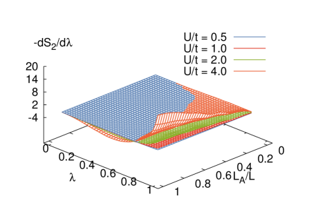
For small subsystems, in addition to relatively small variation, the majority of the deviation from the noninteracting entropy is accumulated at large and appears with mostly uniform signature. Much to the contrary, for larger subsystems, intermediate values of correspond to a region of parameter space that contributes opposite-sign corrections to the entropy, which yields increasing uncertainty as a function of the subsystem size. This effect is most clearly seen for the curve corresponding to the case where the subregion constitutes the entire system. In that case, is zero regardless of the coupling, which means that the integral over must vanish. This happens by a precise cancelation that must be captured by the numerical integration procedure. Given that the features of are roughly concentrated in , we chose the Gauss-Legendre quadrature method to carry out the integral in a precise fashion. Using points in the interval (i.e. 40 points in the defining interval using an even extension of the integrand), we find that, for the parameter values studied here, the systematic effects associated with are smaller than the statistical uncertainty.
Our experience, as detailed above, indicates that the features of are generic: they vary in amplitude with the coupling but are largely insensitive to the overall system size, and generally behave in a benign way as a function of and the sub-system size. Therefore the integration does not contribute to the scaling of the computation time vs. system size beyond a prefactor. Next, we present our results upon integrating over as detailed above.
V.1 Comparison with exact diagonalization results and a first look at statistical effects
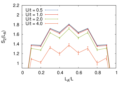
In Fig. 2, we show results for a system of size , where sites and is the lattice spacing (as in conventional Hubbard-model studies). Our results cover couplings = 0.5, 1, 2, and 4, and subsystems of size , which we compare to the results of Ref. Grover . The agreement is quite satisfactory.
To better understand the size of the statistical effects, we also show how our results vary with the number of MC samples in Fig. 3. In Fig. 3 we see that the 25,000 samples collected were well beyond what was needed: half as many would have already given excellent results. These results show that, by including entanglement-sensitive contributions into the probability measure, our approach circumvents the signal-to-noise problem mentioned in the introduction. Below we elaborate more explicitly on statistical effects and said problem, and show concrete numerical examples of how it arises in practice.
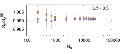
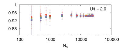
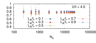
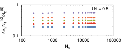
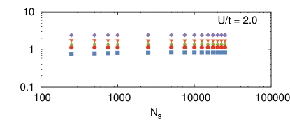
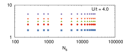
In Fig. 4, we show the overall statistical uncertainty in our estimates of as a function of the number of samples , for the coupling strengths and subsystem sizes studied above. was computed by using the envelope determined by the MC statistical uncertainties in as a function of . While grows with the sub-system size, its scaling remains constant as the number of samples is increased.
V.2 Comparison with naive free-fermion decomposition method
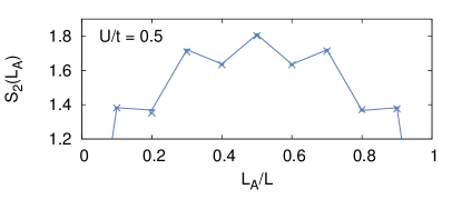

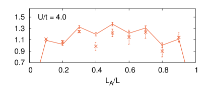
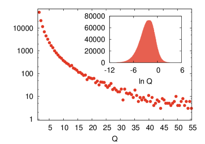
Figure 5 again shows our results for the ten-site Hubbard model using 7,500 decorrelated samples for each value of , this time compared with the naive free-fermion decomposition method using 75,000 samples. Such an increased number of samples for the naive method was chosen to provide a more fair comparison with our method, considering that the latter requires a MC calculation for each value of . We used 20 points but, as explained in more detail below, roughly half of the points require only a small number of samples.
The statistical uncertainties for the naive method do not encompass the expected answers for many of the points, which is a symptom of an “overlap” problem, i.e. the probability measure employed bears little correlation with the observable, as mentioned above (see also Ref. NoiseSignProblemStatistics ). This is the same issue as the signal-to-noise problem referred to above.
To illustrate this situation more precisely, we show in Fig. 6 a histogram of [see Eq. (7)] for and . Even using a logarithmic vertical scale, the distribution displays a long tail that extends across multiple orders of magnitude. We find that the distribution is approximately of the log-normal type (i.e. its logarithm is approximately distributed as a gaussian, as shown in the inset of Fig. 6); this is the challenge faced when attempting to determine the average of with good precision implementing the free-fermion decomposition of Ref. Grover at face value. Moreover, we expect these features to worsen in larger systems, higher dimensions, and stronger couplings, as the matrices involved become more ill-conditioned.
Notably, it is the logarithm of the expectation value of that determines the entanglement entropy, which could then be obtained using the cumulant expansion. However, it is a priori entirely unknown whether such an expansion would converge, i.e. we do not know to what extent this distribution deviates from gaussianity.
The log-normality referred to above has been associated with the auxiliary field representation of the interaction. In such external fields , the orbitals of the trial wavefunction diffuse much like electrons in a disordered medium, and the stronger the interaction (or the lower the temperature) the heavier the tail becomes in the distribution of . This effect was noticed relatively recently in Ref. NoiseSignProblemStatistics , and it appears to be quite ubiquitous. It was then shown, phenomenologically, that many signal-to-noise problems are characterized by the heavy tail of a lognormal distribution (see also, Ref. deGrand ).
V.3 Statistical behavior as a function of coupling, region size, and auxiliary parameter
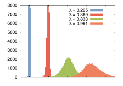
In Fig. 7 we show the statistical distribution of our results for the derivative, for several couplings. The distributions we observe are approximately gaussian (they decay faster than linearly in a log scale), except for the strongest coupling we studied where, not unexpectedly, the distribution becomes more asymmetric and develops heavier tails relative to its weaker-coupling counterparts.
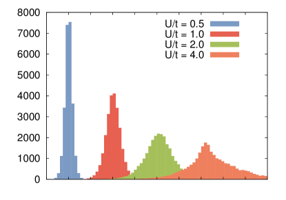
In Fig. 8 we plot the statistical distribution of our results for the derivative at fixed region size and coupling, but varying . As claimed above, the chosen parametrization requires considerably less MC samples at low than at high , as the width of the distributions is much smaller for the former than for the latter.
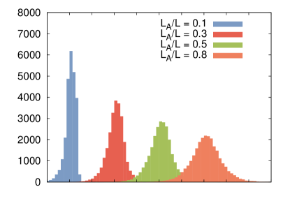
Finally, in Fig. 9 we show the same distribution as above, but as a function of subregion size. As expected, large subregions are more challenging, but the overall shape of the distributions is very well controlled: it is close to gaussian in that its tails decay faster than linearly in a log scale.
VI Summary and Conclusions
In this work, we have put forward an alternative MC approach to the calculation of the Rényi entanglement entropy of many-fermion systems. As an essential feature of our method, we compute the derivative of the entanglement entropy with respect to an auxiliary parameter and integrate afterwards. We have shown that such a derivative can be computed using a MC approach without signal-to-noise issues, as the resulting expression yields a probability measure that does not factor across replicas and accounts for entanglement in the MC sampling procedure in a natural way. The subsequent numerical integration can be carried out efficiently via Gauss-Legendre quadrature.
As a proof of principle, we have presented results for for the 1D Hubbard model at half filling for different coupling strengths and compared with answers obtained by exact diagonalization. Our calculations show that the statistical uncertainties are well controlled, as we have shown in numerous plots and histograms. Although we have not run into numerical stability issues in our tests, we anticipate that those may appear in the form discussed in Ref. Assaad . Our approach is just as general as the one proposed in Ref. Grover . In particular, it can be straightforwardly generalized to finite temperature as well as to relativistic systems, in particular those with gauge fields such as QED and QCD, or any SU() gauge theory.
Acknowledgements.
This work was supported in part by the U.S. National Science Foundation Nuclear Theory Program under Grant No. PHY1306520.References
- (1) L. Amico, R. Fazio, A. Osterloh, and V. Vedral, Rev. Mod. Phys. 80, 517 (2008). R. Horodecki, P. Horodecki, M. Horodecki, K. Horodecki, Rev. Mod. Phys. 81, 865 (2009); J. Eisert, M. Cramer and M. B. Plenio, Rev. Mod. Phys. 82, 277 (2010)
- (2) G. Vidal, J. I. Latorre, E. Rico, and A. Kitaev, Phys. Rev. Lett. 90, 227902 (2003); A. Kitaev and J. Preskill, Phys. Rev. Lett. 96, 110404 (2006); M. Levin and X.-G. Wen, Phys. Rev. Lett. 96, 110405 (2006).
- (3) M. Srednicki, Phys. Rev. Lett. 71, 666 (1993).
- (4) P. Calabrese, J. L. Cardy, J. Stat. Mech. 0406 (2004) P06002.
- (5) C. G. Callan and F. Wilczek, Phys. Lett. B 333, 55 (1994); P. V. Buividovich, M. I. Polikarpov, Nucl. Phys. B 802, 458 (2008); P. Calabrese and J. Cardy, J. Phys. A 42 504005 (2009); T. Nishioka, S. Ryu, T. Takayanagi, J. Phys. A 42, 504008 (2009); M. P. Hertzberg and F. Wilczek Phys. Rev. Lett. 106, 050404 (2011); M. P. Hertzberg, J. Phys. A 46, 015402 (2013).
- (6) R. G. Melko, A. B. Kallin, and M. B. Hastings, Phys. Rev. B 82, 100409 (2010); M. B. Hastings, I González, A. B. Kallin, and R. G. Melko, Phys. Rev. Lett. 104, 157201 (2010); S. V. Isakov, M. B. Hastings, and R. G. Melko, Nature Phys. 7, 772 (2011); R. R. P. Singh, M. B. Hastings, A. B. Kallin, and R. G. Melko, Phys. Rev. Lett. 106, 135701 (2011); S. Inglis and R. G. Melko, Phys. Rev. E 87, 013306 (2013);
- (7) S. Humeniuk and T. Roscilde, Phys. Rev. B 86, 235116 (2012).
- (8) J. McMinis and N. M. Tubman, Phys. Rev. B 87, 081108(R) (2013).
- (9) T. Grover, Phys. Rev. Lett. 111, 130402 (2013).
- (10) D. J. Luitz, X. Plat, N. Laflorencie, and F. Alet, Phys. Rev. B 90, 125105 (2014).
- (11) P. Broecker and S. Trebst, J. Stat. Mech. (2014) P08015.
- (12) L. Wang, M. Troyer, Phys. Rev. Lett. 113, 110401 (2014).
- (13) F. F. Assaad, T. C. Lang, and F. P. Toldin, Phys. Rev. B 89, 125121 (2014); F. F. Assaad, Phys. Rev. B 91, 125146 (2015).
- (14) D. Lee, Phys. Rev. C 78, 024001 (2008); D. Lee, Prog. Part. Nucl. Phys. 63, 117 (2009); F. F. Assaad and H. G. Evertz, Worldline and Determinantal Quantum Monte Carlo Methods for Spins, Phonons and Electrons, in Computational Many-Particle Physics, H. Fehske, R. Shnieider, and A. Weise Eds., Springer, Berlin (2008).
- (15) S. Duane, A. D. Kennedy, B. J. Pendleton, D. Roweth, Phys. Lett. B 195, 216 (1987); S. A. Gottlieb, W. Liu, D. Toussaint, R. L. Renken, Phys. Rev. D 35, 2531 (1987).
- (16) R. M. Neal, MCMC using Hamiltonian dynamics, in Handbook of Markov Chain Monte Carlo, S. Brooks, A. Gelman, G. Jones, and X.-L. Meng Eds., Chapman & Hall / CRC Press, Boca Raton (2011); J. E. Drut and A. N. Nicholson, J. Phys. G: Nucl. Part. Phys. 40, 043101 (2013);
- (17) J. E. Drut and T. A. Lähde, Phys. Rev. Lett. 102, 026802 (2009); Phys. Rev. B 79, 165425 (2009).
- (18) S. Hands and C. Strouthos, Phys. Rev. B 78, 165423 (2008);
- (19) P. V. Buividovich and M. I. Polikarpov, Phys. Rev. B 86, 245117 (2012);
- (20) R. C. Brower, C. Rebbi, and D. Schaich PoS LAT2011, 056 (2012).
- (21) M.-C. Chung and I. Peschel, Phys. Rev. B 64, 064412 (2001); S.-A. Cheong and C. L. Henley, Phys. Rev. B 69, 075111 (2004); I. Peschel, J. Phys. A 36, L205 (2003).
- (22) M. M. Wolf, Phys. Rev. Lett. 96, 010404 (2006); D. Gioev, I. Klich, Phys. Rev. Lett. 96, 100503 (2006); B. Swingle, Phys. Rev. Lett. 105, 050502 (2010); P. Calabrese, M. Mintchev, E. Vicari, Europhys. Lett. 97, 20009 (2012); H. Leschke, A. V. Sobolev, and W. Spitzer, Phys. Rev. Lett. 112, 160403 (2014).
- (23) W. H. Press et al., Numerical Recipes in FORTRAN, (2 Ed., Cambridge University Press, Cambridge, England, 1992).
- (24) M. G. Endres, D. B. Kaplan, J.-W. Lee, A. N. Nicholson, Phys. Rev. Lett. 107, 201601 (2011).
- (25) T. DeGrand, Phys. Rev. D 86, 014512 (2012).