Derivatives of length functions and shearing coordinates on Teichmüller spaces

Abstract.

Let $S$ be a closed oriented surface of genus at least $2$, and denote by $\mathcal{T}(S)$ its Teichmüller space. For any isotopy class of closed curves $\gamma$, we compute the first three derivatives of the length function $\ell_{\gamma}:\mathcal{T}(S)\rightarrow\mathbf{R}_{+}$ in the shearing coordinates associated to a maximal geodesic lamination $\lambda$. We show that if $\gamma$ intersects each leaf of $\lambda$, then the Hessian of $\ell_{\gamma}$ is positive-definite. We extend this result to length functions of measured laminations. We also provide a method to compute higher derivatives of length functions of geodesics. We use Bonahon’s theory of transverse Hölder distributions and shearing coordinates.

Résumé.

Soit $S$ une surface fermée orientable de type hyperbolique, et soit $\mathcal{T}(S)$ son espace de Teichmüller. Étant donnée une classe d’homotopie libre de courbes fermées $\gamma$, nous calculons les trois premières dérivées de la fonction longueur $\ell_{\gamma}:\mathcal{T}(S)\rightarrow\mathbf{R}_{+}$ dans les coordonnées shearing associées à une lamination géodésique maximale $\lambda$ de $S$. Nous montrons que si $\gamma$ intersecte toutes les feuilles de $\lambda$, alors le hessien de $\ell_{\gamma}$ est défini-positif. Nous étendons ce résultat aux fonctions longueur des laminations mesurées. Nous donnons aussi une méthode pour calculer les dérivées d’ordre supérieur de $\ell_{\gamma}$. Nos preuves utilisent les travaux de Bonahon sur les coordonnées shearing.

1. Introduction

Statement of the results

Let $S$ be a closed connected oriented surface with negative Euler characteristic $\chi(S)<0$. Its Teichmüller space $\mathcal{T}(S)$ is the space of hyperbolic metrics on $S$ up to isotopy. It is a smooth manifold of dimension $-3\chi(S)$. Given a non trivial isotopy class of closed curves $\gamma$, there is a smooth length function $\ell_{\gamma}:\mathcal{T}(S)\rightarrow\mathbf{R}_{+}^{\ast}$ that associates to a point $[m]$ in $\mathcal{T}(S)$ the length $\ell_{\gamma}(m)$ of the unique $m$-geodesic in $\gamma$. These length functions play a crucial role in low-dimensional topology and geometry.

In this article, we study the derivatives of length functions in the shearing coordinates. Given a maximal geodesic lamination $\lambda$ on $S$, Bonahon ([Bon96]) realized $\mathcal{T}(S)$ as an open convex cone $\mathcal{C}(\lambda)$ in the linear space $\mathcal{H}(\lambda;\mathbf{R})$ of transverse Hölder distributions for $\lambda$ . The linear structure of $\mathcal{H}(\lambda;\mathbf{R})$ is meaningful in terms of hyperbolic geometry. If $\mu$ is a transverse measure for $\lambda$, the trajectories of the earthquake flow directed by $\mu$ are affine lines in the shearing coordinates. Thus, the linear flow in $\mathcal{C}(\lambda)$ can be seen as a generalization of the earthquake flow.

Our main theorem gives explicit formulas for the first and second derivatives of length functions in the shearing coordinates:

Theorem 1.1.

Let $[m]$ be a point in $\mathcal{T}(S)$, $\lambda$ be a maximal geodesic lamination, and $\gamma$ be a closed geodesic transverse to $\lambda$. For any transverse Hölder distribution $\alpha\in\mathcal{H}(\lambda;\mathbf{R})$, we have

$$(\mathrm{d}\ell_{\gamma})_{[m]}(\alpha) = \int_{\gamma}\cos\theta_{p}\ \mathrm{d}\alpha(p),$$

$$(\mathrm{d}^{2}\ell_{\gamma})_{[m]}(\alpha,\alpha) = \frac{1}{2\sinh\frac{\ell_{\gamma}}{2}}\int_{\gamma}\int_{\gamma}\cosh\left(\frac{\ell_{\gamma}}{2}-\ell_{pq}\right)\sin\theta_{p}\sin\theta_{q}\ \mathrm{d}\alpha(p)\mathrm{d}\alpha(q),$$

where we denote by $\theta_{p}$ the $m$-angle at $p$ from $\gamma$ to the leaf of $\lambda$ passing through $p$ following the orientation of $S$, and by $\ell_{pq}$ the $m$-length of any of the two segments of $\gamma$ bounded by $p$ and $q$.

Remarks.

1. We identify the tangent space $T_{[m]}\mathcal{T}(S)$ with $\mathcal{H}(\lambda;\mathbf{R})$.

2. The support of $\alpha$ on $\gamma$ is contained in $\gamma\cap\lambda$, so that the formulas above make sense.

3. When $\gamma$ is a closed leaf of $\lambda$, then its length is given by the Theorem E of [Bon96].

These are generalizations of classical formulas for the first and second derivatives of length functions along earthquake deformations (Kerckhoff [Ker83], Wolpert [Wol81, Wol83]). Note that a generic geodesic lamination admits only one transverse measure (up to multiplication by a positive scalar), therefore the formulas of Kerckhoff and Wolpert give (generically) the derivatives of length functions for only one direction in the shearing coordinates.

We also provide a method to compute recursively the higher derivatives of $\ell_{\gamma}$, and we give an explicit formula for the third derivative (§4). It seems possible to find a closed formula for all derivatives using our method. Recently, Bridgeman ([Bri]) gave a closed formula for all derivatives of $\cosh(\ell_{\gamma}/2)$ along twist deformations. Our method of computation is different in that we use Jacobi fields instead of product of matrices in $\mathsf{SL}(2,\mathbf{C})$.

We extend the formula for the first derivative to length functions of measured laminations (Theorem 5.1), and we show that:

Theorem 1.2.

If $(\gamma,\mu)$ is a measured lamination that intersects each leaf of $\lambda$, then the Hessian of $\ell_{(\gamma,\mu)}$ in the shearing coordinates is everywhere positive-definite.

Remark.

This is not an obvious consequence of the previous theorem, for positive transverse Hölder distributions are exactly transverse measures (Bonahon [Bon97, Proposition 18]).

Actually, we give an effective lower bound for the Hessian of $\ell_{(\gamma,\mu)}$ (Proposition 6.3). It was already known that, under the hypothesis of the theorem, the function $\ell_{(\gamma,\mu)}$ is strictly convex in the shearing coordinates (Bestvina-Bromberg-Fujiwara-Souto [BBFS13] for the case of closed geodesics, and Théret [Thé14] for the case of measured laminations).

As well-known, the Teichmüller space admits a noncomplete metric of negative sectional curvature, called the Weil-Petersson metric. Recently, Wolf ([Wol12]) found an explicit formula for the Weil-Petersson Hessian of a geodesic length function, which was already known to be positive-definite (Wolpert [Wol87, Theorem 4.6]). As observed by G. Mondello, one part of Wolf’s formula is very similar to our formula. This could be explained as follows: this part of Wolf’s formula comes from the second variation of the geodesic seen as a curve on $S$ ([Wol12, §2]), and the idea of our computations (§7) is precisely to move the endpoints of a geodesic arc on a fixed hyperbolic surface.

In this article, we only deal with the closed oriented surface $S$. However, our results extend to any compact surfaces with negative Euler characteristic by considering a double cover which is closed and orientable.

Ideas and heuristic

There are different presentations of the shearing coordinates (see for instance [BBFS13]). We use the one given by Bonahon ([Bon96]), where the shearing coordinates of a hyperbolic metric are encoded by a transverse Hölder distribution. This is a crucial point as our proofs are based on the fact that a transverse Hölder distribution $\alpha\in\mathcal{H}(\lambda;\mathbf{R})$ is locally approximated by a sequence $(\alpha_{n})_{n}$ of linear combinations of Dirac measures. Here locally means that this approximation works only for the restriction of $\alpha$ to a given arc. In particular, it is not an approximation in $\mathcal{H}(\lambda;\mathbf{R})$. Our main theorem comes quickly once we have clearly stated this approximation (Lemma 3.1).

Let us give some heuristic proof of the main theorem. We identify the geodesic $\gamma$ with an element of $\pi_{1}(S)$ still denoted $\gamma$. Let $(A,m_{A})$ be the hyperbolic annulus which is the cover of $(S,m)$ with respect to the subgroup $\langle\gamma\rangle$ of $\pi_{1}(S)$. The leaves of $\lambda$ that intersect $\gamma$ lift to a lamination $\lambda_{A}$ of $(A,m_{A})$. Working in the annulus $(A,m_{A})$ has two advantages:

1. in the space $\mathcal{H}(\lambda_{A};\mathbf{R})$ the Hölder distribution which is the restriction of $\alpha$ to $\gamma$ can be approximated by a sequence $(\alpha_{n})_{n}$ of linear combinations of Dirac measures. So, for any Hölder function $f$ on $\gamma$, we have $\int_{\gamma}f\mathrm{d}\alpha_{n}\rightarrow\int_{\gamma}f\mathrm{d}\alpha$ as $n$ tends to infinity.

2. there is a bijection between the leaves of $\lambda_{A}$ and the intersection points of $\lambda$ with $\gamma$.

The Hölder distribution $\alpha_{n}$ can be written $\alpha_{n}=a_{1}\delta_{l_{1}}+\ldots+a_{n}\delta_{l_{n}}$ where the $l_{i}$’s are some leaves of the lamination $\lambda_{A}$. We associate to $\alpha_{n}$ a deformation $t\mapsto m^{t\alpha_{n}}_{A}$ of $m_{A}$ obtained by shearing along each $l_{i}$ by an amount equal to $ta_{i}$. The derivative of $\ell_{\gamma}$ along the this deformation is given by $\left[\frac{\mathrm{d}}{\mathrm{d}t}\ell_{\gamma}(m^{t\alpha_{n}}_{A})\right]_{t}=\int_{\gamma}\left[\cos\theta_{p}\right]_{m^{t\alpha_{n}}_{A}}\mathrm{d}\alpha_{n}(p)$, where the bracket means that the angle is evaluated with respect to the metric $m_{A}^{t\alpha_{n}}$. From the work of Bonahon, we find that $\left[\frac{\mathrm{d}}{\mathrm{d}t}\ell_{\gamma}(m^{t\alpha_{n}}_{A})\right]_{t}$ converges uniformly to $\left[\frac{\mathrm{d}}{\mathrm{d}t}\ell_{\gamma}(m^{t\alpha}_{A})\right]_{t}$ as $n$ tends to infinity, where $t\mapsto m_{A}^{t\alpha}$ is the deformation defined by $\alpha$. Using the convergence of $(\alpha_{n})_{n}$ towards $\alpha$, we conclude that $\left[\frac{\mathrm{d}}{\mathrm{d}t}\ell_{\gamma}(m^{t\alpha}_{A})\right]_{0}=\int_{\gamma}\cos\theta_{p}\mathrm{d}\alpha$.

In the rest of the paper, following Bonahon ([Bon96]), we work in the universal cover $(\tilde{S},\tilde{m})$ instead of the annulus $(A,m_{A})$ used in [BBFS13]. Note that $\mathcal{H}(\lambda_{A};\mathbf{R})$ and $\mathcal{T}(A)$ have infinite dimension, and consequently are not well-adapted to differential calculus.

Organization of the paper

We first take some pages to recall Bonahon’s theory of transverse Hölder distributions and shearing coordinates (§2). Then, we define the sequence $(\alpha_{n})_{n}$, and show its convergence towards $\alpha$ (§3). This enables us to compute the derivatives of the length functions in the shearing coordinates, in particular we prove the main theorem (§4). In §5 we consider the possible extensions of these results to length functions of measured laminations. Finally, we show the positivity of the Hessian of the length functions (§6). We postpone in §7 the computations of the derivatives of some geometric quantities along twist deformations.

Acknowlegments

I would like to thank Andrea Sambusetti for his support.

2. Transverse Hölder distributions and shearing coordinates

Here we introduce transverse Hölder distributions and shearing coordinates following the work of Bonahon ([Bon96, Bon97], see also [Bon01, §1]). We closely follow his notations, and sometimes his text.

Geodesic laminations

Given a hyperbolic metrics $m^{\prime}$ on $S$, the identity map between $(\tilde{S},\tilde{m})$ and $(\tilde{S},\tilde{m}^{\prime})$ is a quasi-isometry, which extends to an equivariant homeomorphism between the visual compactifications. As a consequence, the boundary at infinity $\tilde{S}_{\infty}$ is a purely topological object, and so is the space of geodesics of $\tilde{S}$ defined by

$$G(\tilde{S})=(\tilde{S}_{\infty}\times\tilde{S}_{\infty}-\Delta)/\mathbf{Z}_{2},$$

where $\Delta$ is the diagonal, and $\mathbf{Z}_{2}$ acts by permuting the factors. We transparently identify a geodesic with its unordered pair of limit points.

A geodesic lamination $\lambda$ on $S$ is a collection of disjoint simple $m$-geodesics whose union is closed in $S$. Its lift $\tilde{\lambda}$ is a $\pi_{1}(S)$-invariant closed subset of $G(\tilde{S})$.

Transverse Hölder distributions

Let $(X,d)$ be a metric space. A function $f:X\rightarrow\mathbf{R}$ is Hölder continuous if there exists some constants $A>0$ and $1\geq\nu>0$ such that:

$$|f(x)-f(y)|\leq A\ d(x,y)^{\nu}\quad\forall x,y\in X.$$

We denote by $H_{\nu}(X;K)$ the linear space of Hölder continuous functions with exponent $1\geq\nu>0$, and support contained in a compact subset $K\subset X$. We equip $H_{\nu}(X;K)$ with the norm $\|\cdot\|_{\nu}$ defined by:

$$\|f\|_{\nu} = \|f\|_{\infty}+\sup_{x,y\in X}\frac{|f(x)-f(y)|}{d(x,y)^{\nu}}.$$

There is a continuous injection $H_{\nu}(X;K)\rightarrow H_{\nu^{\prime}}(X;K^{\prime})$ for any $\nu\geq\nu^{\prime}$, and any $K\subset K^{\prime}$. We denote by $H(X)$ the space of Hölder continuous functions on $X$ with compact support, it is the union of all $H_{\nu}(X;K)$ with $1\geq\nu>0$ and $K\subset X$ compact. A Hölder distribution on $X$ is a linear form on $H(X)$ whose restriction to each $H_{\nu}(X;K)$ is continuous. A (positive) Radon measure is a very particular example of Hölder distribution.

Let $\lambda$ be a geodesic lamination on $(S,m)$. A transverse Hölder distributions $\alpha$ for $\lambda$ is a Hölder distribution on each smooth arc transverse to $\lambda$ such that: if $H$ is a Hölder bicontinuous homotopy preserving $\lambda$ between two transverse arcs $k$ and $k^{\prime}$, then $H$ transports the Hölder distribution on $k$ to the one on $k^{\prime}$. This invariance property implies that the support of the Hölder distribution on $k$ is contained in $\lambda\cap k$. A transverse Hölder distribution which is a Radon measure on each transverse arc is called a transverse measure.

We denote by $\mathcal{H}(\lambda;\mathbf{R})$ the linear space of transverse Hölder distributions for $\lambda$. It is finite dimensional, we precisely have $\dim\mathcal{H}(\lambda;\mathbf{R})=\dim\mathcal{T}(S)=-3\chi(S)$ when $\lambda$ is maximal. By comparison, the dimension of the cone of transverse measures for $\lambda$ does not exceed $-\frac{3}{2}\chi(S)$.

Geodesic Hölder currents

Transverse Hölder distributions and transverse measures are of topological nature. To see that they do not depend on the metric $m$, we interpret them as objects defined on the space of geodesics $G(\tilde{S})$. This space has a canonical Hölder structure. The $\tilde{m}$-angle at a point $x$ in $\tilde{S}$ defines a metric on $\tilde{S}_{\infty}$, and consequently on $G(\tilde{S})$. A different choice for $m$ or $x$ would change the metric on $G(\tilde{S})$, but not its Hölder class.

A geodesic Hölder current (resp. a geodesic current) on $S$ is a $\pi_{1}(S)$-invariant Hölder distribution (resp. Radon measure) on $G(\tilde{S})$. Given a geodesic lamination $\lambda$, transverse Hölder distributions (resp. transverse measures) for $\lambda$ are in one-to-one correspondance with geodesic Hölder currents (resp. geodesic currents) whose support is contained in $\tilde{\lambda}$.

Shearing coordinates

Let us fix a maximal geodesic lamination $\lambda$. The complement of $\tilde{\lambda}$ in $(\tilde{S},\tilde{m})$ is a disjoint union of ideal triangles. The way these ideal triangles are glued together is encoded by a transverse Hölder distribution $\sigma_{m}\in\mathcal{H}(\lambda;\mathbf{R})$, which depends only on the isotopy class of $m$. The correspondence $m\mapsto\sigma_{m}$ induces a real analytic homeomorphism

$$\Sigma:\mathcal{T}(S)\longrightarrow\mathcal{C}(\lambda),$$

whose image $\mathcal{C}(\lambda)$ is an open convex cone in $\mathcal{H}(\lambda;\mathbf{R})$ bounded by finitely many faces. The transverse measures for $\lambda$ belong to the boundary of $\mathcal{C}(\lambda)$.

When defining the shearing coordinates ([Bon96, §2]), Bonahon uses transverse cocycles instead of transverse Hölder distributions. These two concepts are equivalent ([Bon97, §6]).

Shearing hyperbolic metrics

Given $\alpha\in\mathcal{H}(\lambda;\mathbf{R})$, the most natural deformation of $\sigma_{m}$with tangent direction $\alpha$ is $t\mapsto\sigma_{m}+t\alpha$. When $\alpha$ is a transverse measure for $\lambda$, this deformation remains in $\mathcal{C}(\lambda)$ for all $t\geq 0$, and its pull-back $t\mapsto\Sigma^{-1}(\sigma_{m}+t\alpha)$ to $\mathcal{T}(S)$ coincide with the trajectory of the earthquake flow passing through $[m]$ and pointing in the direction of $\alpha$. Now, we assume $\alpha$ sufficiently small, and we explain how to construct a hyperbolic metric $m^{\alpha}$ such that

$$[m^{\alpha}] = \Sigma^{-1}(\sigma_{m}+\alpha).$$

First, we deform the action by Deck transformations of $\pi_{1}(S)$ on $\tilde{S}$ into a discrete and faithful action $\rho^{\alpha}:\pi_{1}(S)\rightarrow\mathsf{Isom}(\tilde{S})$. The quotient $(S^{\prime},m^{\prime})=(\tilde{S},\tilde{m})/\rho^{\alpha}$ is a hyperbolic surface. Then, we define $m^{\alpha}$ as the pull-back of $m^{\prime}$ by any diffeomorphism $f:S\rightarrow S^{\prime}$ whose induced homomorphism on fundamental groups is $\rho^{\alpha}$. The isotopy class $[m^{\alpha}]\in\mathcal{T}(S)$ does not depend on $f$. We take few lines to recall the construction of $\rho^{\alpha}$.

Given two components $P$ and $Q$ of $\tilde{S}-\tilde{\lambda}$, we denote by $\mathcal{P}_{PQ}$ the set of components of $\tilde{S}-\tilde{\lambda}$ that separate $P$ from $Q$. For any $R\in\mathcal{P}_{PQ}$, we call $g_{R}^{P}$ (resp. $g_{R}^{Q}$) the boundary geodesic of $R$ in the direction of $P$ (resp. of $Q$). We also set $\alpha(P,R)=\alpha(\mathbf{1}_{k})$ where $k$ is any geodesic arc in $(\tilde{S},\tilde{m})$ with endpoints in $P$ and $R$.

To each finite subset $\mathcal{P}\subset\mathcal{P}_{PQ}$, we associate the isometry $\varphi^{\alpha}_{\mathcal{P}}\in\mathsf{Isom}(\tilde{S})$ defined by:

$$\varphi^{\alpha}_{\mathcal{P}} = T^{\alpha(P,P_{1})}_{g_{1}^{P}}T^{-\alpha(P,P_{1})}_{g_{1}^{Q}}\ T^{\alpha(P,P_{2})}_{g_{2}^{P}}T^{-\alpha(P,P_{2})}_{g_{1}^{Q}}\ldots T^{\alpha(P,P_{n})}_{g_{n}^{P}}T^{-\alpha(P,P_{n})}_{g_{n}^{Q}}T^{\alpha(P,Q)}_{g_{Q}^{P}},$$

where the $\mathcal{P}_{i}$’s are the elements of $\mathcal{P}$ indexed as one goes from $P$ to $Q$, and $T^{u}_{g}$ is the $\tilde{m}$-isometry that translates by a signed length $u$ on the geodesic $g$. We assume that the geodesics that separate $P$ and $Q$ are oriented from right to left seen from $P$. The sequence $(\varphi^{\alpha}_{\mathcal{P}})_{\mathcal{P}}$ converges in $\mathsf{Isom}(\tilde{S})$, we call $\varphi^{\alpha}_{PQ}$ its limit ([Bon96, §5]).

To define $\rho^{\alpha}$, we fix a component $P$ of $\tilde{S}-\tilde{\lambda}$, and we set

$$\rho^{\alpha}(\gamma) = \varphi^{\alpha}_{P\gamma(P)}\circ\gamma,$$

for every $\gamma\in\pi_{1}(S)$. The conjugacy class of $\rho^{\alpha}$ does not depend on the fixed component $P$.

Uniform convergence of derivatives

In this paragraph, we discuss the convergence of the derivatives of some geometric quantities. Here $\ell(\cdot)$ stands for the translation length.

Lemma 2.1.

As $\mathcal{P}$ tends to $\mathcal{P}_{P\gamma(P)}$, the derivatives of $\alpha\mapsto\ell(\varphi^{\alpha}_{\mathcal{P}}\circ\gamma)$ converge towards the derivatives of $\alpha\mapsto\ell(\varphi^{\alpha}_{PQ}\circ\gamma)$ uniformly on some neighborhood of the origin in $\mathcal{H}(\lambda;\mathbf{R})$.

Consequence 2.1.

To compute the derivatives of $\alpha\mapsto\ell_{\gamma}(m^{\alpha})$, it suffices to compute the derivatives of $\alpha\mapsto\ell(\varphi^{\alpha}_{\mathcal{P}_{n}}\circ\gamma)$, and determine their limits.

Sketch of proof.

We take a complex path following Bonahon ([Bon96, §10]). We use the complexifcation $\mathcal{H}(\lambda;\mathbf{R})\oplus i\mathcal{H}(\lambda;\mathbf{R}/2\pi\mathbf{Z})$ of $\mathcal{H}(\lambda;\mathbf{R})$, where $\mathcal{H}(\lambda;\mathbf{R}/2\pi\mathbf{Z})$ is the space of transverse Hölder distributions with values in $\mathbf{R}/2\pi\mathbf{Z}$. Without entering into details, let us mention that $\mathcal{C}(\lambda)\oplus\mathcal{H}(\lambda;\mathbf{R}/2\pi)$ parametrizes pleated surfaces with pleating locus $\lambda$ (see [Bon96, Theorem 31] for a precise statement).

We identify $\tilde{S}$ with $\mathbf{H}^{2}$. For each $\mathcal{P}$, the map

$$\begin{array}[]{lrll}\varphi_{\mathcal{P}}:&\mathcal{H}(\lambda;\mathbf{R})&\longrightarrow&\mathsf{Isom}^{+}(\mathbf{H}^{2})\\ &\alpha&\longmapsto&\varphi_{\mathcal{P}}^{\alpha}\end{array},$$

extends to a holomorphic map

$$\begin{array}[]{lrll}\varphi_{\mathcal{P}}:&\mathcal{H}(\lambda;\mathbf{R})\oplus i\mathcal{H}(\lambda;\mathbf{R}/2\pi\mathbf{Z})&\longrightarrow&\mathsf{Isom}^{+}(\mathbf{H}^{3})\simeq\mathsf{PSL}(2;\mathbf{C})\\ &\alpha+i\beta&\longmapsto&\varphi_{\mathcal{P}}^{\alpha+i\beta}\end{array}.$$

Bonahon showed (see the proof of [Bon96, Theorem31]) that the sequence $(\alpha+i\beta\mapsto\varphi_{\mathcal{P}}^{\alpha+i\beta})_{\mathcal{P}}$ converges uniformly on a small neighborhood of the origin, and deduce that ${\alpha+i\beta}\mapsto\varphi^{\alpha+i\beta}_{PQ}$ is holomorphic on this neighborhood. We use Cauchy’s formula to conclude. ∎

We identify $\tilde{S}$ with $\mathbf{H}^{2}$. The same line of arguments gives:

Lemma 2.2.

Let $z\in\partial\mathbf{H}^{2}$ be an endpoint of some leaf $l\in\tilde{\lambda}$. We denote by $\mathcal{P}_{l}$ the set of components of $\mathbf{H}-\tilde{\lambda}$ that separate $P$ from $l$. As $\mathcal{P}\subset\mathcal{P}_{l}$ tends to $\mathcal{P}_{l}$, the derivatives of $\alpha\mapsto\varphi^{\alpha}_{\mathcal{P}}(z)$ converge uniformly on a small neighborhood of the origin in $\mathcal{H}(\lambda;\mathbf{R})$ .

Sketch of proof.

If $l$ is an isolated leaf of $\tilde{\lambda}$, then it bounds a component $R$ of $\mathbf{H}-\tilde{\lambda}$ such that $\mathcal{P}_{l}=\mathcal{P}_{PR}$. In that case, the lemma is obvious as $(\alpha+i\beta\mapsto\varphi^{\alpha+i\beta}_{\mathcal{P}})_{\mathcal{P}\subset\mathcal{P}_{l}}$ converges uniformly to $\alpha+i\beta\mapsto\varphi_{PR}^{\alpha+i\beta}$.

If $l$ is not an isolated leaf, then we consider a sequence of endpoints $(z_{n})_{n}$ of isolated leaves that converges monotonically to $z$. We denote by $z_{n}^{\alpha+i\beta}$ the limit of $(\varphi^{\alpha+i\beta}_{\mathcal{P}}(z_{n}))_{\mathcal{P}\subset\mathcal{P}_{l_{n}}}$, where $l_{n}$ is the isolated leaf with endpoint $z_{n}$. By monotonicity, the sequence $(z_{n}^{\alpha})_{n}$ converges for $\alpha\in\mathcal{H}(\lambda;\mathbf{R})$ small enough. Moreover, the convergence is uniform on some neighborhood of the origin in $\mathcal{H}(\lambda;\mathbf{R})$, thanks to Dini’s theorem. We endow $\partial\mathbf{H}^{3}\simeq\mathbf{S}^{2}$ with the round metric compatible with the elliptic elements of $\mathsf{Isom}(\mathbf{H}^{3})$. From the definition of $\varphi_{\mathcal{P}}^{\alpha+i\beta}$, it comes that $d_{\mathbf{S}^{2}}(z^{\alpha+i\beta}_{n},z_{m}^{\alpha+i\beta})\leq d_{\mathbf{S}^{2}}(z^{\alpha}_{n},z_{m}^{\alpha})$. We deduce that the sequence $(\alpha+i\beta\mapsto z_{n}^{\alpha+i\beta})_{n}$ is uniformly Cauchy on some neighborhood of the origin in $\mathcal{H}(\lambda;\mathbf{R})\oplus i\mathcal{H}(\lambda;\mathbf{R}/2\pi\mathbf{Z})$. This implies immediately the uniform convergence of the derivatives, for each $z_{n}$ is holomorphic. It is then not difficult to conclude. ∎

The interest of this lemma lies in the fact that many geometric quantities can be expressed in terms of points on the boundary. Let $p,q,r,s$ be four points on $\partial\mathbf{H}^{2}$. If the geodesics $(qr)$ and $(ps)$ intersect with an angle $\theta$, then the cross-ratio $[p,q,r,s]$ is equal to $\cos^{2}(\theta/2)$. If they do not intersect, then $[p,q,r,s]=-\sinh^{2}(h/2)$, where $h$ is the distance between the geodesics.

An example

The shearing coordinates measure how the components of $S-\lambda$ are glued together. We did not define the map $\Sigma$ that associates the transverse Hölder distribution $\sigma_{m}$ to the hyperbolic metric $m$, but we explained how to pass from the hyperbolic metric $m$ to the hyperbolic metric $m^{\alpha}$ with shearing coordinates $\sigma_{m}+\alpha$. This is done by shifting the components of $\tilde{S}-\tilde{\lambda}$ with respect to each other. In this paragraph, we illustrate this construction by considering the case of a finite maximal geodesic lamination.

2pt $P_{0}$ [tl] at 320 80 $P_{1}$ [tl] at 360 80 $Q_{0}$ [tl] at 545 80 $Q_{1}$ [tl] at 495 80 $g_{0}$ [tl] at 295 150 $g_{1}$ [tl] at 332 150 $g_{2}$ [tl] at 372 150 $h_{0}$ [tl] at 562 150 $h_{1}$ [tl] at 530 150 $h_{2}$ [tl] at 487 150

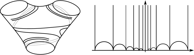
Figure 1. A finite maximal lamination

Let $\lambda$ be a finite maximal geodesic lamination, obtained by adding spiralling geodesics to some pants decomposition (see for instance the picture on the left of Figure 1). We assume that the geodesics spiral in the same direction along each closed leaf of $\lambda$. We identify $(\tilde{S},\tilde{m})$ with the upper-half plane, in such a way that $\tilde{\lambda}$ contains a bi-infinite sequence of vertical geodesics converging to the imaginary axis (as on the right of Figure 1). The imaginary axis is the lift of some closed leaf $\gamma$ of $\lambda$, and the other vertical geodesics are lifts of the geodesics spiralling along $\gamma$. We denote by $g_{0},g_{1},\ldots$ the vertical geodesics on the left of the imaginary axis, indexed from left to right. We denote by $P_{i}$ the component of $\tilde{S}-\tilde{\lambda}$ bounded by $g_{i}$ and $g_{i+1}$. We define similarly $h_{i}$ and $Q_{i}$.

Given a transverse Hölder distribution $\alpha$ for $\lambda$, we observe that

$$\varphi^{\alpha}_{P_{0}P_{n}} = T^{\alpha(P_{0},P_{1})}_{g_{1}}T^{\alpha(P_{1},P_{2})}_{g_{2}}\cdots T^{\alpha(P_{n-1},P_{n})}_{g_{n}}.$$

Adjacent components are shifted with respect to each other, and the amount of shifting is given by the $\alpha$-measure of a small geodesic arc intersecting their common boundary. When the $\alpha$-measure of this arc is positive, the components are shifted to the left with respect to each other. Then, we recognize the classical construction of an earthquake path.

One would expect the sequence of isometries $(\psi^{\alpha}_{n})_{n}$ defined by

$$\psi^{\alpha}_{n} = T^{\alpha(P_{0},P_{1})}_{g_{1}}\cdots T^{\alpha(P_{n-1},P_{n})}_{g_{n}}T^{\alpha(Q_{n},Q_{n-1})}_{h_{n}}\cdots T^{\alpha(Q_{1},Q_{0})}_{h_{1}},$$

to converge towards $\varphi^{\alpha}_{P_{0}Q_{0}}$. However, we have $T_{g_{i}}^{\alpha(P_{i-1},P_{i})}(z)=e^{\alpha(P_{i-1},P_{i})}z+\ast$, and

$$\psi_{n}^{\alpha}(z) = e^{\alpha(P_{0},P_{n})+\alpha(Q_{0},Q_{n})}z+\ast,$$

where $\ast$ replaces any constant term. So, the convergence of $\alpha(P_{0},P_{n})+\alpha(Q_{0},Q_{n})$ as $n$ tends to infinity is a necessary condition for the convergence of $(\psi^{\alpha}_{n})_{n}$. This is automatically satisfied when $\alpha$ is a transverse measure, but not in general. On the contrary we have

$$\varphi_{\mathcal{P}}^{\alpha}(z) = e^{\alpha(P_{0},Q_{0})}z+\ast,$$

for $\mathcal{P}=\{P_{1},\ldots,P_{n},Q_{n},\ldots,Q_{1}\}$. This explains Bonahon’s choice for the sequence $(\varphi^{\alpha}_{\mathcal{P}})_{\mathcal{P}}$.

We conclude this paragraph with a remark on the length function of the closed leaf $\gamma$. The spiralling geodesics divide a pair of pants into two ideal triangles. It implies that $P_{2}=\gamma(P_{0})$, where $\gamma\in\pi_{1}(S)$ translates along the imaginary axis. With some abuse of notations, we use the letter $\gamma$ for an element of $\pi_{1}(S)$ whose axis project on the geodesic $\gamma$. The axis of $\rho^{\alpha}(\gamma)$ is still a vertical geodesic, and its translation length $\ell_{\gamma}(m^{\alpha})$ is equal to the logarithm of the ratio between the Euclidean widths of $P_{0}$ and $\varphi^{\alpha}_{P_{0}P_{2}}(P_{2})$. So we find that

$$\ell_{\gamma}(m^{\alpha}) = \ell_{\gamma}(m)+\alpha(P_{0},P_{2}).$$

We also have $\ell_{\gamma}(m^{\alpha})=\ell_{\gamma}(m)+\alpha(Q_{0},Q_{2})$. The quantity $\alpha(P_{0},P_{2})$ is the $\alpha$-mass of some geodesic loop homotopic to $\gamma$ and transverse to $\lambda$. The formula above is a particular case of the theorem E of [Bon96].

3. Local approximation

Once for all, we fix a hyperbolic metric $m$ on $S$, a maximal geodesic lamination $\lambda$ of $S$, and a transverse Hölder distribution $\alpha\in\mathcal{H}(\lambda;\mathbf{R})$. We consider a geodesic arc $k$ of $(\tilde{S},\tilde{m})$ whose endpoints belong to two components $P$ and $Q$ of $\tilde{S}-\tilde{\lambda}$. We denote by $K\subset G(\tilde{S})$ the compact subset containing the leaves of $\tilde{\lambda}$ that separate $P$ from $Q$.

Let $(\mathcal{P}_{n})_{n}$ be an increasing sequence of finite subsets that converges to $\mathcal{P}_{PQ}$, we assume for simplicity that $\mathcal{P}_{n}$ is of cardinal $n$. The isometry $\varphi_{\mathcal{P}_{n}}^{\alpha}$ is encoded by the following Hölder distribution on $G(\tilde{S})$:

$$\alpha_{n} = \alpha(P,Q)\ \delta_{g^{P}_{Q}}+\sum_{i=1}^{n}\alpha(P_{1},P_{i})\ (\delta_{g_{i}^{P}}-\delta_{g_{i}^{Q}}).$$

We underline that $\alpha_{n}$ has finite support, and is not $\pi_{1}(S)$-invariant.

We call $\alpha_{K}$ the restriction of the geodesic Hölder current $\alpha$ to $H(K)$. The first lemma below says that $(\alpha_{n})_{n}$ is a good approximation of $\alpha_{K}$. In particular, $\alpha$ can be approximated locally by linear combinations of Dirac measures. This is certainly not possible in $\mathcal{H}(\lambda;\mathbf{R})$ in general. The second lemma gives an application of the previous result to functions defined by an integral depending on a parameter.

Convergence of the sequence

This lemma is due to Bonahon ([Bon97, Lemma 9]), but we include a proof as it plays a fundamental role in this article, and as Bonahon’s formulation is slightly different.

Lemma 3.1.

The sequence $(\alpha_{n})_{n}$ converges to $\alpha_{K}$ in the topological dual of any $H_{\nu}(K)$ with $1\geq\nu>0$.

Remark 3.1.

The proof uses the geometry of the geodesic lamination $\lambda$ on $(S,m)$.

Proof following Bonahon’s ideas.

We consider $\alpha$ and $\alpha_{n}$ as Hölder distributions on $k$ whose supports are included in $k\cap\tilde{\lambda}$. It is equivalent to work in $H(K)$ or in $H(k)$ (this is justified by [Bon97, Lemma 2], and the proof of the Proposition 5 in [Bon97]).

We index the elements $P_{1},P_{2},\ldots,P_{n},\ldots$ of $\mathcal{P}_{PQ}$ in such a way that the sequence of $\tilde{m}$-lengths $(\ell(k\cap P_{n}))_{n}$ is non-increasing. Then, we set $\mathcal{P}_{n}=\{P_{1},\ldots,P_{n}\}$, and we prove the lemma for this particular sequence $(\mathcal{P}_{n})_{n}$. This clearly suffices to establish the lemma for any sequence $(\mathcal{P}_{n})_{n}$ of finite subsets of $\mathcal{P}_{PQ}$ that is increasing and tends to $\mathcal{P}_{PQ}$.

For any $f\in H_{\nu}(k)$ we have ([Bon96, Theorem 2]):

$$|(\alpha-\alpha_{n})(f)| \leq \sum_{i\geq n}\alpha(P_{1},P_{i})\ |f(x_{P_{i}}^{P})-f(x_{P_{i}}^{Q})|,$$

where $x^{P}_{P_{i}}$ and $x_{P_{i}}^{Q}$ are the endpoints of $k\cap P_{i}$. Using the following estimates

$$\left\{\begin{array}[]{llll}d_{\tilde{m}}(x_{P_{i}}^{-},x_{P_{i}}^{+})&\leq&Be^{-Ai}&\textnormal{\cite[cite]{[\@@bibref{}{bonahon-toulouse}{}{}, Lemma~{}5]}}\\ \alpha(P_{1},P_{i})&\leq&C\|\alpha\|i&\textnormal{\cite[cite]{[\@@bibref{}{bonahon-toulouse}{}{}, Lemma~{}6]}}\end{array}\right.,$$

we find

$$|(\alpha-\alpha_{n})(f)| \leq C\|\alpha\|\ B^{\nu}\|f\|_{\nu}\left(\sum_{i\geq n}i\ e^{-\nu Ai}\right),$$

where $A,B,C>0$ are independent of $f$, and $\|\cdot\|$ is a norm on $\mathcal{H}(\lambda;\mathbf{R})$. Clearly, the norm of $\alpha-\alpha_{N}$ in the topological dual of $H_{\nu}(k)$ tends to zero as $n$ tends to infinity. ∎

Application to functions defined through transverse Hölder distributions

Let us recall that we have fixed a point in $\tilde{S}_{\infty}$, and that the $\tilde{m}$-angle at this point induces a Riemannian metric on $G(\tilde{S})$. Actually $G(\tilde{S})$ equipped with this metric is the interior of a flat Mœbius band with geodesic boundary.

We denote by $g$ the geodesic of $(\tilde{S},\tilde{m})$ that supports $k$. The endpoints of $g$ divide $\tilde{S}_{\infty}$ into two open intervals, and their product is in bijection with the open subset $U\subset G(\tilde{S})$ that contains all geodesics intersecting $g$ transversely. It is easy to find a product of two compact subintervals whose image in $G(\tilde{S})$ contains $K$ in its interior. This gives a compact and convex subset $C$ that contains $K$ in its interior.

We consider a smooth function $f:V\times U\rightarrow\mathbf{R}$, where $V\subset\mathbf{R}^{m}$ is an open subset. We define the functions $F_{n}:V\rightarrow\mathbf{R}$ and $F:V\rightarrow\mathbf{R}$ by:

$$\left\{\begin{array}[]{lll}F_{n}(p)&=&\int_{K}f(p,q)\ \mathrm{d}\alpha_{n}(q)\\ F(p)&=&\int_{K}f(p,q)\ \mathrm{d}\alpha(q)\end{array}\right.\textnormal{for any }p\in V.$$

Note that any function $f(p,\cdot)$ is Lipschitz on $K$ as $f$ is smooth, so that the expressions above make sense. We observe easily that $F_{n}$ is smooth with

$$(\mathrm{d}^{k}F_{n})_{p}(u) = \int_{K}\partial_{p}^{k}f(p,\cdot)(u)\ \mathrm{d}\alpha_{n}$$

for any $p\in V$ and $u\in(\mathbf{R}^{m})^{k}$.

Lemma 3.2.

The function $F$ is smooth, and $(F_{n})_{n}$ converges to $F$ in $C^{\infty}(V;\mathbf{R})$, equipped with the topology of uniform convergence of all derivatives on compact subsets. Moreover

$$(\mathrm{d}^{k}F)_{p}(u) = \int_{K}\partial_{p}^{k}f(p,\cdot)(u)\ \mathrm{d}\alpha$$

for any $p\in V$ and $u\in(\mathbf{R}^{m})^{k}$.

Proof.

For any $p\in V$, and any $u\in(\mathbf{R}^{m})^{k}$ of unit norm, we have:

$$|(\mathrm{d}^{k}F_{n})_{p}(u)-\alpha_{K}(\partial^{k}_{p}f(p,\cdot)(u))| \leq \|\alpha_{K}-\alpha_{n}\|_{1}\ \|\partial^{k}_{p}f(p,\cdot)(u)\|_{1}.$$

But, when $p$ belongs to a compact subset $A\subset V$, we have the uniform bound:

$$\|\partial^{k}f(p,\cdot)(u)\|_{1} \leq \sup_{A\times C}\|\partial^{k}_{p}f\|+\sup_{A\times C}\|\partial_{q}\partial^{k}_{p}f\|,$$

where we use the generic symbol $\|\cdot\|$ for the norms induced by the Riemannian norm on the spaces of multilinear forms on some tangent space. We conclude that $(\mathrm{d}^{k}F_{n})_{n}$ converges uniformly by applying the previous lemma. ∎

4. Computations of the derivatives of length functions

We fix a closed geodesic $\gamma$ that is transverse to $\lambda$. We are going to compute the first three derivatives of $\ell_{\gamma}$ in the shearing coordinates.

We consider a geodesic arc $k$ which is a lift of the geodesic $\gamma$. Following the notations of the previous section, we assume that the endpoints of $k$ belong to two components $P$ and $Q$ of $\tilde{S}-\tilde{\lambda}$, and we denote by $g$ the geodesic of $(\tilde{S},\tilde{m})$ supporting $k$.

In all the formulas below, geometric quantities as $\ell_{\gamma}$ or $\cos\theta_{p}$ have to be evaluated with respect to the fixed metric $m$.

Auxiliary derivatives

We recall that $U$ is the open subset of $G(\tilde{S})$ that consists in the geodesics intersecting $g$ transversely. We introduce the function $\theta:\mathcal{T}(S)\times U\rightarrow\mathbf{R}/2\pi\mathbf{Z}$ that associates to a point $[m^{\prime}]\in\mathcal{T}(S)$, and a geodesic $h\in U$, the oriented $\tilde{m}^{\prime}$-angle $\theta_{h}$ between $g$ and $h$. We assume that $g$ is going from $P$ to $Q$, and that $h$ points to the left when crossed by $g$. The function $\theta$ is clearly smooth. We do not specify the metric in the notation $\theta_{h}$, because in all the formulas below the angle is measured with respect to $\tilde{m}$.

Lemma 4.1.

Let $\alpha\in\mathcal{H}(\lambda;\mathbf{R})$. For any intersection point $p\in\gamma\cap\lambda$, we have

$$(\mathrm{d}\cos\theta_{p})_{[m]}(\alpha) = \frac{\sin\theta_{p}}{2\sinh\frac{\ell_{\gamma}}{2}}\ \int_{\gamma}\cosh\left(\frac{\ell_{\gamma}}{2}-\ell_{pq}\right)\sin\theta_{q}\ \mathrm{d}\alpha(q),$$

$$(\mathrm{d}\sin\theta_{p})_{[m]}(\alpha) = -\frac{\cos\theta_{p}}{2\sinh\frac{\ell_{\gamma}}{2}}\ \int_{\gamma}\cosh\left(\frac{\ell_{\gamma}}{2}-\ell_{pq}\right)\sin\theta_{q}\ \mathrm{d}\alpha(q),$$

where $\ell_{\gamma}$ is the $m$-length of $\gamma$. For any pair of intersection points $\{p,q\}\subset\gamma\cap\lambda$, we have

$$(\mathrm{d}\ell_{pq})_{[m]}(\alpha) = \int_{p}^{q}\cos\theta_{r}\mathrm{d}\alpha(r)$$

$$+\frac{1}{2\sinh\frac{\ell_{\gamma}}{2}}\int_{\gamma}\sinh\left(\frac{\ell_{\gamma}}{2}-\ell_{rq}\right)\sin\theta_{r}\cot\theta_{q}-\sinh\left(\frac{\ell_{\gamma}}{2}-\ell_{rp}\right)\sin\theta_{r}\cot\theta_{p}\mathrm{d}\alpha(r),$$

where, given an orientation for $\gamma$, we denote by $\ell_{pq}$ the $m$-length of the segment of $\gamma$ that goes from $p$ to $q$.

Remark 4.1.

We have $\ell_{\gamma}/2-\ell_{pq}=\ell_{\gamma}/2-(\ell_{\gamma}-\ell_{qp})=-(\ell_{\gamma}/2-\ell_{qp})$, so that the first two formulas do not depend on an orientation of $\gamma$.

Proof.

The three formulas rely on the same ideas, so we only prove the first one. We work in the universal cover, and we integrate Hölder distributions over the set $K$ defined at the beginning of §3. This is the same as integrating over $\gamma$.

As we work in the universal cover, we can consider the variation of a geometric quantity in the direction of a finite approximation $\alpha_{n}$. We recall that $\alpha_{n}$ is a linear combination of Dirac measures. The deformation associated to $\alpha_{n}$ is obtained by shifting along each leaf of $\tilde{\lambda}$ that belong to the support of $\alpha_{n}$, and the amount of shifting is equal to the corresponding coefficient of the linear combination. For instance, the $\alpha_{n}$-displacement of the component $Q$ is given by $t\mapsto\varphi^{t\alpha}_{\mathcal{P}_{n}}(Q)$.

We denote by $f_{n}:[-\varepsilon,\varepsilon]\rightarrow\mathbf{R}$ (resp. $f:[-\varepsilon,\varepsilon]\rightarrow\mathbf{R}$) the variation of $\cos\theta_{p}$ in the direction of $\alpha_{n}$ (resp. of $\alpha$). Note that $f(t)$ is equal to $\cos\theta_{p}$ evaluated with respect to the metric $m^{t\alpha}$. From the Lemme 2.2, we deduce the pointwise convergence of the derivatives of $f_{n}$ towards the derivatives of $f$ as $n$ tends to infinity.

We have computed at the end of §7 the derivative $f^{\prime}_{n}$. It is given by the first formula above with $\alpha_{n}$ instead of $\alpha$, and $K$ instead of $\gamma$. We conclude by taking the limit of $f^{\prime}_{n}(0)$ as $n$ tends to infinity (Lemma 3.1).

As regard the other formulas, let us precise that in the computation of the derivative of $\ell_{pq}$, one has to take into account the contribution of the geodesics of $K$ lying between $p$ and $q$. The formula (6) works only for the leaves that do not lie between $p$ and $q$. One establishes easily a formula for the other case, using the same ideas as for the proof of the formula (6). ∎

The first and second derivatives

The last formula of the above lemma implies

$$(\mathrm{d}\ell_{\gamma})_{[m]}(\alpha) = \int_{\gamma}\cos\theta_{p}\ \mathrm{d}\alpha(p),$$

for all $\alpha\in\mathcal{H}(\lambda;\mathbf{R})$. Then, the first formula and the Lemma 3.2 give

$$(\mathrm{d}^{2}\ell_{\gamma})_{[m]}(\alpha,\beta) = \frac{1}{2\sinh\frac{\ell_{\gamma}}{2}}\int_{\gamma}\int_{\gamma}\cosh\left(\frac{\ell_{\gamma}}{2}-\ell_{pq}\right)\ \sin\theta_{p}\sin\theta_{q}\ \mathrm{d}\beta(q)\mathrm{d}\alpha(p),$$

for all $\alpha,\beta\in\mathcal{H}(\lambda;\mathbf{R})$.

Higher derivatives

The Lemmas 4.1 and 3.2 enable the computations of all derivatives of $\ell_{\gamma}$ in a recursive way. As an example, this is the formula for the third derivative:

$$(\mathrm{d}^{3}\ell_{\gamma})_{[m]}(\alpha^{3}) =-\frac{1}{2\left(\sinh\frac{\ell_{\gamma}}{2}\right)^{2}}\int_{\gamma}\int_{\gamma}\int_{\gamma} \cosh(\ell_{pr}-\ell_{rq})\sin\theta_{p}\sin\theta_{q}\cos\theta_{r}$$

$$+\cosh(\ell_{qp}-\ell_{pr})\cos\theta_{p}\sin\theta_{q}\sin\theta_{r}$$

$$+\cosh(\ell_{pq}-\ell_{qr})\sin\theta_{p}\cos\theta_{q}\sin\theta_{r} \ \mathrm{d}\alpha^{3},$$

for all $\alpha\in\mathcal{H}(\lambda;\mathbf{R})$. This should be compared with Bridgeman’s formula for the third derivative of $2\cosh(\ell_{\gamma}/2)$ along twist deformations ([Bri]).

5. Extension to measured laminations

In this section, we prove the following generalization of our main theorem:

Theorem 5.1.

Let $\lambda$ be a maximal geodesic lamination of $(S,m)$, and $(\gamma,\mu)$ be a measured lamination transverse to $\lambda$. For any transverse Hölder distribution $\alpha\in\mathcal{H}(\lambda;\mathbf{R})$, we have

$$(\mathrm{d}\ell_{(\gamma,\mu)})_{[m]}(\alpha) = \int\int\cos\theta_{p}\ \mathrm{d}\mu\ \mathrm{d}\alpha(p).$$

Moreover, if $\{(\gamma_{n},\mu_{n})\}_{n}$ is a sequence of weighted simple closed geodesics that converges to $(\gamma,\mu)$ in the space of measured laminations $\mathcal{ML}(S)$, then the derivatives of $\ell_{(\gamma_{n},\mu_{n})}$ converge pointwise towards the derivatives of $\ell_{(\gamma,\mu)}$ as $n$ tends to infinity:

$$\lim_{n\rightarrow\infty}(\mathrm{d}^{k}\ell_{(\gamma_{n},\mu_{n})})_{[m]}(\alpha_{1},\ldots,\alpha_{k}) = (\mathrm{d}^{k}\ell_{\gamma})_{[m]}(\alpha_{1},\ldots,\alpha_{k}),$$

for any $k\geq 0$ and any $\alpha_{1},\ldots,\alpha_{k}\in\mathcal{H}(\lambda;\mathbf{R})$.

Remark 5.1.

To find a formula for the second derivative of $\ell_{(\gamma,\mu)}$, one has to extend $\ell_{pq}$ to measured laminations, and to study its regularity.

Question 5.1.

It would be interesting to look at the case of geodesic currents.

In the first paragraph, we give sense to the integral above. In the other paragraphs, we show that the derivatives of $\ell_{(\gamma_{n},\mu_{n})}$ converge pointwise towards the derivatives of $\ell_{(\gamma,\mu)}$ as $n$ tends to infinity. It is then easy to prove the formula.

In what follows, we introduce some sets $U$ and $K_{R}$ that are different from the sets $U$ and $K$ seen previously. For simplicity, we assume that the geodesic lamination $\gamma$ is minimal.

Definition of the integral

Let $U$ be the open subset of $G(\tilde{S})\times G(\tilde{S})$ consisting in couples of intersecting geodesics. We consider a smooth function $f:\mathcal{T}(S)\times U\rightarrow\mathbf{R}$, which is invariant with respect to the diagonal action of $\pi_{1}(S)$ on $U$. Let us give sense to the following integral:

$$\int_{l\in\lambda}\int_{g\in\gamma}f(m,g,l)\ \mathrm{d}\mu(g)\mathrm{d}\alpha(l),$$

We fix an oriented geodesic arc $s$, which is disjoint from $\lambda$ and intersects $\gamma$ transversely. We choose $s$ pointing towards a cusp of $S-\lambda$. The closure of each component of $\gamma-s$ is a geodesic arc with endpoints in $s$. We partition these arcs according to their isotopy class relative to $s$. We denote by $\mathcal{R}$ the set of such isotopy classes, which is finite since all these arcs are pairwise disjoint.

We fix a class $R\in\mathcal{R}$, and we choose two lifts $\tilde{s}_{1}$ and $\tilde{s}_{2}$ of $s$ to $\tilde{S}$, such that any geodesic arc in $R$ admits a lift with endpoints in $\tilde{s}_{1}$ and $\tilde{s}_{2}$. We denote by $K_{R}\subset G(\tilde{S})$ the set of geodesics that intersects $\tilde{s}_{1}$ and $\tilde{s}_{2}$. We call $h_{1}$ and $h_{2}$ the geodesics supporting $\tilde{s}_{1}$ and $\tilde{s}_{2}$. We denote by $V_{R}$ the open subset of $G(\tilde{S})$ that consists in the geodesics lying between $h_{1}$ and $h_{2}$ that intersect any geodesic in $K_{R}$. We define $F^{R}:\mathcal{T}(S)\times V_{R}\rightarrow\mathbf{R}$ as follows:

$$F^{R}(m,l) = \int_{\tilde{\gamma}\cap K_{R}}f(m,g,l)\ \mathrm{d}\mu(g).$$

This integral is well defined ($\tilde{\gamma}\cap K_{R}$ is a compact subset of $G(\tilde{S})$) and does not depend on the choice of any lift. From a classical theorem of Lebesgue, the function $F^{R}$ is smooth. Thus $l\mapsto F^{R}(m,l)$ is Hölder, and $\int_{\tilde{\lambda}\cap V^{R}}F^{R}(m,l)\mathrm{d}\alpha$ is well-defined. We set

$$F(m)\ :=\ \int_{l\in\lambda}\int_{g\in\gamma}f(g,l,m)\ \mathrm{d}\mu(g)\ \mathrm{d}\alpha(l)\ :=\ \sum_{\mathcal{R}}\int_{\tilde{\lambda}\cap V_{R}}F^{R}(m,l)\ \mathrm{d}\alpha(l).$$

The function $F:\mathcal{T}(S)\rightarrow\mathbf{R}$ is smooth (Lemma3.2).

From simple closed geodesics to measured laminations

We consider a sequence $\{(\gamma_{n},\mu_{n})\}_{n}$ of weighted simple closed geodesics that converges to $(\gamma,\mu)$ in $\mathcal{ML}(S)$. We assume that each geodesic $\gamma_{n}$ intersects $s$, and that the arcs made of the components of $\gamma_{n}-s$ belong to the classes in $\mathcal{R}$. The existence of such a sequence is obvious when working in the train track which has a unique switch correponding to $s$, and one edge for each $R\in\mathcal{R}$.

As above, we have a well-defined and smooth function $F_{n}^{R}:\mathcal{T}(S)\times V_{R}\rightarrow\mathbf{R}$ given by:

$$F^{R}_{n}(m,l)=\int_{g\in K_{R}}f(m,g,l)\mathrm{d}\mu_{n}(g).$$

The restriction of $\mu_{n}$ to $K_{R}$ is a linear combination of Dirac measures, so this integral is actually a finite sum. As $\mu_{n}$ tends to $\mu$ in the space of Radon measures on $G(\tilde{S})$, it comes that $F_{n}^{R}$ converges to $F^{R}$ uniformly on compact subsets of $\mathcal{T}(S)\times V_{R}$. Similarly, any derivative of the form $(\partial_{m}^{k}F_{n}^{R})_{(m,l)}(\alpha_{1},\ldots,\alpha_{k})$ ($k\geq 0$ and $\alpha_{1},\ldots,\alpha_{k}\in\mathcal{H}(\lambda;\mathbf{R})$) converges towards $(\partial_{m}^{k}F^{R})_{(m,l)}(\alpha_{1},\ldots,\alpha_{k})$ uniformly on compact subsets of $\mathcal{T}(S)\times V_{R}$. This implies the $1$-Hölder convergence of all derivatives, for the Lipschitz constant of a smooth function is equal to the supremum of its derivative. We deduce that

$$(\mathrm{d}^{k}F)_{[m]}(\alpha_{1},\ldots,\alpha_{k}) = \lim_{n\rightarrow\infty}(\mathrm{d}^{k}F_{n})_{[m]}(\alpha_{1},\ldots,\alpha_{k}),$$ (1)

for any $k\geq 0$ and any $\alpha_{1},\ldots,\alpha_{k}\in\mathcal{H}(\lambda;\mathbf{R})$.

Proof of Theorem 5.1

We take $f$ defined by $f(g,l,m)=\cos\theta(g,l,m)$, where $\theta(g,l,m)$ is the $\tilde{m}$-angle going from $g$ to $h$ following the orientation of $\tilde{S}$. According to our main theorem we have $(\mathrm{d}\ell_{(\gamma_{n},\mu_{n})})_{[m]}(\alpha)=F_{n}(m)$. And, in the paragraph above, we have seen that $\lim_{n\rightarrow\infty}F_{n}(m)\ =\ F(m)$, where the convergence is uniform on compact subsets of $\mathcal{T}(S)$. As $(\ell_{(\gamma_{n},\mu_{n})})_{n}$ converges pointwise to $\ell_{(\gamma,\mu)}$, we conclude that $(\mathrm{d}\ell_{(\gamma,\mu)})_{[m]}(\alpha)\ =\ F(m).$

We remark that the formula (1) gives the pointwise convergence of all derivatives of $\ell_{(\gamma_{n},\mu_{n})}$ towards the derivatives of $\ell_{(\gamma,\mu)}$ as $n$ tends to infinity.

6. Positivity of the Hessian

In this section, we give a proof of Theorem 1.2. We interpret

$$\int_{\gamma}\int_{\gamma}\cosh\left(\frac{\ell_{\gamma}}{2}-\ell_{pq}\right)\sin\theta_{p}\sin\theta_{q}\ \mathrm{d}\alpha_{n}^{2},$$

as a quadratic form evaluated at $\alpha_{n}$, seen as a vector in some finite dimensional linear space. Using an easy lemma of linear algebra, we find an effective lower bound for the integral above. This lower bound increases with $n$.

A lemma on symmetric matrices with nonnegative entries

This lemma is certainly well-known, but we were not able to find it in the litterature.

Lemma 6.1.

Let $(a_{ij})_{1\leq i,j\leq n}$ be a symmetric matrix satisfying the following conditions:

1. $a_{ij}\geq 0$ for all $i,j$ ($A$ is nonnegative),

2. $a_{ii}>a_{ij}$ for all $i,j$.

Then $A$ is definite-positive, that is $x^{t}Ax>0$ for any $x\in\mathbf{R}^{n}-\{0\}$.

Consequence 6.1.

If we replace the condition $ii)$ by the weaker condition $a_{ii}\geq a_{ij}$ ($\forall i,j$), then we find that $A$ is positive, that is $x^{t}Ax\geq 0$ for any $x\in\mathbf{R}^{n}$. Thus, for any $x\in\mathbf{R}^{n}$ we have $x^{t}Ax\geq d_{1}x_{11}^{2}+\ldots+d_{n}x_{nn}^{2}$, where $d_{i}=\min\{x_{ii}-x_{ij}~{};~{}j\neq i\}$.

Proof.

We perform the Gauss elimination process to get an upper-triangular matrix which has same leading principal minors as $A$. Let us recall that this process consists in $n$ steps, and that the $k^{\textnormal{th}}$ step gives a matrix $A^{[k+1]}$, obtained from $A^{[k]}$ by doing the operation

$$L_{i}-\frac{a^{[k]}_{ik}}{a^{[k]}_{kk}}L_{k}\rightarrow L_{i}$$

for any $i>k$. This operation preserves the leading principal minors. By construction, any diagonal entry $a^{[k]}_{ii}$ of $A^{[k]}$ ($k\geq 2$) remains greater than any other entry of the same line, in particular is positive as $0=a^{[k]}_{i1}$. We conclude that the upper-triangular matrix $A^{[n+1]}$ has positive diagonal entries, thus all its leading principal minors are positive, and $A$ is positive according to Sylvester criterion. ∎

Positivity of the Hessian

Lemma 6.2.

Let $\gamma$ be a closed geodesic of $(S,m)$. Let $x_{1},\ldots,x_{N}$ be isolated points of $\gamma\cap\lambda$, and denote by $\varepsilon_{i}$ be the minimal distance on $\gamma$ between $x_{i}$ and any other point of $\gamma\cap\lambda$. For any transverse Hölder distribution $\alpha\in\mathcal{H}(\lambda;\mathbf{R})$, we have

$$(\mathrm{d}^{2}\ell_{\gamma})_{[m]}(\alpha^{2}) \geq \sum_{i=1}^{N}\sinh(\ell_{\gamma}/2-\varepsilon_{i})\ \varepsilon_{i}\ \alpha(x_{i})^{2}\ \sin^{2}\theta_{x_{i}},$$

where $\alpha(x_{i})$ is the $\alpha$- measure of a small arc of $\gamma$ that intersects $\lambda$ only at $x_{i}$.

Proof.

Following the notations of §2 and §3, we fix a geodesic segment $k\subset\tilde{S}$ which is a lift of $\gamma$ whose endpoints belong to two components $P$ and $Q$ of $\tilde{S}-\tilde{\lambda}$. To any intersection point $x_{i}$ corresponds a unique isolated leaf $p_{i}$ of $\tilde{\lambda}$ that separates $P$ from $Q$.

Each $p_{i}$ is adjacent to two components of $\tilde{S}-\tilde{\lambda}$. For $n$ big enough, the set $\mathcal{P}_{n}$ contains all the components adjacent to the $p_{i}$’s. Thus, the corresponding Hölder distribution $\alpha_{n}$ can be written in the form $\alpha_{n}=\sum_{i=1}^{n}b_{i}\delta_{p_{i}}$ with $b_{i}=\alpha(x_{i})$ for $i\leq N$, and $p_{i}\neq p_{j}$ for $i\neq j$. We explicitly have

$$\int_{k^{2}}\cosh(\ell_{\gamma}/2-\ell_{pq})\sin\theta_{p}\sin\theta_{q}\ \mathrm{d}\alpha_{n}^{2} = B^{t}HB,$$

where $H$ is the $n\times n$ symmetric matrix given by $H_{ij}=\cosh(\ell_{\gamma}/2-\ell_{p_{i}p_{j}})$, and $B$ is the vector $B=(b_{1}\sin\theta_{p_{1}},\ldots,b_{n}\sin\theta_{p_{n}})$. Let $\varepsilon_{i}$ be the minimal distance on $k$ between $p_{i}$ and any other leaf of $\tilde{\lambda}$. Note that $\varepsilon_{i}$ is positive if and only if $p_{i}$ is an isolated leaf of $\tilde{\lambda}$. For any $p_{i}$ ($1\leq i\leq n$) and any $q\in\tilde{\lambda}$ we have

$$\cosh(\ell_{\gamma}/2)-\cosh(\ell_{\gamma}/2-\ell_{p_{i}q})\ \geq\ \cosh(\ell_{\gamma}/2)-\cosh(\ell_{\gamma}/2-\varepsilon_{i})\ \geq\ \sinh(\ell_{\gamma}/2-\varepsilon_{i})\varepsilon_{i}.$$

We write $H=H^{\prime}+D$ where $D$ is the diagonal matrix with $D_{ii}=\sinh(\ell/2-\varepsilon_{i})\varepsilon_{i}$. According to Consequence 6.1, the matrix $H^{\prime}$ is positive and

$$\int_{k^{2}}\cosh(\ell_{\gamma}/2-\ell_{pq})\sin\theta_{p}\sin\theta_{q}\ \mathrm{d}\alpha_{n}^{2} \geq \sum_{i=1}^{n}D_{ii}B_{i}^{2},$$

$$\geq \sum_{i=1}^{N}\sinh(\ell_{\gamma}/2-\varepsilon_{i})\varepsilon_{i}\ \alpha(x_{i})^{2}\ \sin^{2}\theta_{p_{i}}.$$

This proves the lemma as the right-hand side of the inequality does not depend on $n$. ∎

Using the Theorem 5.1, we easily extend the lemma above to measured laminations by considering a sequence of simple closed geodesics converging to $(\gamma,\mu)$.

Proposition 6.3.

Let $s_{1},\ldots,s_{N}$ be disjoint geodesic arcs of $(S,m)$ that are supported by isolated leaves of $\lambda$. For each $i$, we denote by $\varepsilon_{i}>0$ the biggest $\varepsilon>0$ such that any geodesic arc of length $\varepsilon$ starting at a point in $s_{i}$ has no other intersection point with $\lambda$ (except if it is contained in $\lambda$). Let $(\gamma,\mu)$ be a measured lamination. For any $\alpha\in\mathcal{H}(\lambda;\mathbf{R})$ we have

$$(\mathrm{d}^{2}\ell_{(\gamma,\mu)})_{[m]}(\alpha^{2}) \geq \sum_{i=1}^{N}\sinh(\ell_{(\gamma,\mu)}/2-\varepsilon_{i})\ \varepsilon_{i}\ \alpha(s_{i})^{2}\ \int_{s_{i}}\sin^{2}\theta_{x}\mathrm{d}\mu(x),$$

where $\alpha(s_{i})$ is the $\alpha$-measure of a small geodesic arc intersecting $s_{i}$.

7. Shearing along one geodesic

In the hyperbolic plane $\mathbf{H}$, we consider two disjoint non asymptotic geodesics $h$ and $h^{\prime}$. We fix an isometry $\gamma$ whose axis $g$ intersect both geodesics, and such that $\gamma(h)=h^{\prime}$. The geodesic $g$ has an orientation given by $\gamma$, and we orient every geodesic intersecting $g$ in such a way that it points to the left when crossed by $g$. Let $\varphi(t)$ be the isometry of $\mathbf{H}$ that translates by a signed length $t$ on $h^{\prime}$. We set $\gamma(t):=\varphi(t)\circ\gamma$, and we denote by $g(t)$ the axis of $\gamma(t)$.

The quotient $\mathbf{H}/\langle\gamma(t)\rangle$ is a hyperbolic annulus. By construction, both geodesics $h$ and $h^{\prime}$ project onto the same complete simple geodesic, and the deformation $t\mapsto\mathbf{H}/\langle\gamma(t)\rangle$ is obtained by shearing along this geodesic.

Given a geodesic $l$ of $\mathbf{H}$ lying between $h$ and $h^{\prime}$ and intersecting $g$, we want to compute the variations of the intersection point $g(t)\cap l$, and of the angle $\theta_{l}(t)$ between $g(t)$ and $l$. This enables the computation of the first and second derivatives of the translation length $\ell(t):=\ell(\gamma(t))$. We stress that $h$, $h^{\prime}$ and $l$ are fixed, but that the axis $g(t)$ moves with $t$.

Description of the configuration

Let $[a,a^{\prime}]$ be the unique geodesic segment orthogonal to $h$ and $h^{\prime}$ at its endpoints. Given a geodesic $l$ lying between $h$ and $h^{\prime}$ and intersecting $g$, we denote by $f_{l}(t)$ the signed distance on $l$ between $l\cap[a,a^{\prime}]$ and $l\cap g(t)$.

As $h^{\prime}$ is the image of $h$ by any $\gamma(t)$, we have $\theta_{h}(t)=\theta_{h^{\prime}}(t)$ for any $t$. Thus the points $a$ and $a^{\prime}$ are at the same distance from $g(t)$ on respectively $h$ and $h^{\prime}$. It follows that $f_{h}(t)=f_{h}(0)-\frac{t}{2}$ and $f_{h^{\prime}}(t)=f_{h^{\prime}}(0)+\frac{t}{2}$, in particular

$$f_{h}^{\prime} \equiv -\frac{1}{2}.$$ (2)

This implies that the midpoint $M$ of $[a,a^{\prime}]$ belongs to $g(t)$ independently of $t$. Therefore $g(t)$ is obtained by rotating $g(0)$ by an angle $\rho(t)$ about $M$.

2pt $h$ at 70 460 $h^{\prime}$ at 360 460 $l$ at 210 460 $g(t)$ at 260 500 $M$ at 210 570 $a$ at 65 560 $a^{\prime}$ at 340 562 $\theta_{h}(t)$ at 95 650

Figure 2. Configuration

Variation of the translation length

The translation length $\ell$ is equal to the distance between the intersection point of $g(t)$ with $h$ and $h^{\prime}$. The gradient field of the function $d_{\mathbf{H}}(M,\cdot)$ consists in the unit vectors pointing in the direction opposite to $M$. We deduce easily from (2) that

$$\ell^{\prime} = \cos\theta_{h}.$$ (3)

It is geometrically clear that $\theta_{h}$ is strictly increasing, so we already find $\ell^{\prime\prime}\geq 0$.

Variation of the intersection point

We are interested in the trajectory of the point $g(t)\cap l$ on the fixed geodesic $l$.We recall that $g(t)$ is obtained by rotating $g(0)$ by an angle $\rho(t)$ about the midpoint of $[a,a^{\prime}]$. As well-known, if $p(t)$ is a point moving by an angle $\rho(t)$ on a circle of radius $r$ in $\mathbf{H}$, then its velocity $p^{\prime}(t)$ is equal to $\rho^{\prime}(t)\sinh(r)$ times the vector tangent to the circle at $p(t)$ pointing in the positive direction. This gives

$$f_{l}^{\prime} = \rho^{\prime}\ \frac{\sinh\left(\frac{\ell}{2}-\ell_{hl}\right)\ }{\sin\theta_{l}},$$

where $\ell_{hl}(t)$ is the distance on $g(t)$ from $h$ to $l$. Taking $l=h$ we find

$$f_{h}^{\prime} = \rho^{\prime}\ \frac{\sinh(\frac{\ell}{2})}{\sin\theta_{h}}.$$ (4)

Equations (2) and (4) enable us to express the angular velocity $\rho^{\prime}$ in terms of $\ell$ and $\theta_{h}$. We finally obtain:

$$f_{l}^{\prime} = -\frac{1}{2}\frac{\sin\theta_{h}}{\sin\theta_{l}}\frac{\sinh(\frac{\ell}{2}-\ell_{hl})}{\sinh\frac{\ell}{2}}.$$ (5)

Variation of the distance between two intersection points

Let $l^{\prime}$ be another geodesic of $\mathbf{H}$ lying between $l$ and $h^{\prime}$, and intersecting $g$. As we know the gradient of the distance function $d_{\mathbf{H}}(\cdot,\cdot)$, and the variation of each of the intersection points $l\cap g(t)$ and $l^{\prime}\cap g(t)$, we easily compute

$$\ell^{\prime}_{ll^{\prime}} = \frac{\sin\theta_{h}}{2\sinh\frac{\ell}{2}}\left(\sinh(\frac{\ell}{2}-\ell_{hl^{\prime}})\cot\theta_{l^{\prime}}-\sinh(\frac{\ell}{2}-\ell_{hl})\cot\theta_{l}\right)$$ (6)

Variation of the angle, second variation of the translation length

We now consider only $l$. We remark that

$$\cos\theta_{l}(t) = \pm\langle l^{\prime}_{p(t)},Z_{p(t)}\rangle,$$

where $p(t)=l\cap\gamma(t)$, $l^{\prime}$ is the unit vector field tangent to $l$, and $Z$ is the unit vector field pointing in the direction of the midpoint $M$ of $[a,a^{\prime}]$. Note that we have $p^{\prime}(t)=f_{l}^{\prime}(t)l^{\prime}_{p(t)}$. As $l^{\prime}$ is parallel, we find

$$\pm\frac{\mathrm{d}\cos\theta_{l}}{\mathrm{d}t}(t) = \langle(\nabla_{f_{l}^{\prime}l^{\prime}}l^{\prime})_{p(t)},Z_{p(t)}\rangle+\langle l^{\prime}_{p(t)},(\nabla_{f^{\prime}_{l}l^{\prime}}Z)_{p(t)}\rangle$$

$$= f_{l}^{\prime}\langle l^{\prime},(\nabla_{l^{\prime}}Z)_{p(t)}\rangle$$

By definition of Jacobi fields we have:

$$(\nabla_{l^{\prime}}Z)_{p(t)} = -J^{\prime}(d_{\mathbf{H}}(M,p(t))),$$

where $s\mapsto J(s)$ is the Jacobi field along the geodesic segment $[M,p(t)]$ satisfying $J(0)=0$ and $J(d(M,p(t))=l^{\prime}_{p(t)}$. According to the classical formula for the norm of Jacobi fields in hyperbolic spaces we have:

$$\|J^{\prime}(s)^{\perp}\| = \sin\theta_{l}\ \frac{\sinh(s)}{\sinh(d_{\mathbf{H}}(M,p(t)))},$$

where $\perp$ means the component orthogonal to $[M,p(t)]$. We finally find

$$\frac{\mathrm{d}\cos\theta_{l}}{\mathrm{d}t} = -f^{\prime}_{l}\ \sin^{2}\theta_{l}\ \coth(d_{\mathbf{H}}(M,g\cap l)),$$

$$= \frac{1}{2}\ \frac{\cosh(\frac{\ell}{2}-\ell_{hl})}{\sinh\frac{\ell}{2}}\ \sin\theta_{h}\sin\theta_{l}.$$

This is also equal to the second variation of the translation length because $\ell^{\prime}=\cos\theta_{h}$. We have already proved that $\ell^{\prime\prime}\geq 0$, so there is no sign issue.

References

- [BBFS13] M. Bestvina, K. Bromberg, K. Fujiwara, and J. Souto. Shearing coordinates and convexity of length functions on Teichmüller space. Amer. J. Math., 135(6):1449–1476, 2013.
- [Bon96] F. Bonahon. Shearing hyperbolic surfaces, bending pleated surfaces and Thurston’s symplectic form. Ann. Fac. Sci. Toulouse Math. (6), 5(2):233–297, 1996.
- [Bon97] F. Bonahon. Transverse Hölder distributions for geodesic laminations. Topology, 36(1):103–122, 1997.
- [Bon01] F. Bonahon. Geodesic laminations on surfaces. In Laminations and foliations in dynamics, geometry and topology (Stony Brook, NY, 1998), volume 269 of Contemp. Math., pages 1–37. AMS, 2001.
- [Bri] M. Bridgeman. Higher derivatives of length functions along earthquakes deformations. Michigan Math. J. To appear.
- [Ker83] S. Kerckhoff. The Nielsen Realization Problem. Ann. Math. (2), 117(2):235–265, 1983.
- [Thé14] G. Théret. Convexity of length functions and Thurston’s shear coordinates. Available on the server arXiv, 2014.
- [Wol81] S. Wolpert. An elementary formula for the Fenchel-Nielsen twist. Comment. Math. Helv., 56(1):132–135, 1981.
- [Wol83] S. Wolpert. On the symplectic geometry of deformations of a hyperbolic surface. Ann. of Math. (2), 117(2):207–234, 1983.
- [Wol87] S. Wolpert. Geodesic length functions and the Nielsen problem. J. Differential Geom., 25(2):275–296, 1987.
- [Wol12] M. Wolf. The Weil-Petersson Hessian of length on Teichmüller space. J. Differential Geom., 91(1):129–169, 2012.