Nonparametric estimates of pricing functionals

Abstract

We analyze the empirical performance of several non-parametric estimators of the pricing functional for European options, using historical put and call prices on the S&P500 during the year 2012. Two main families of estimators are considered, obtained by estimating the pricing functional directly, and by estimating the (Black-Scholes) implied volatility surface, respectively. In each case simple estimators based on linear interpolation are constructed, as well as more sophisticated ones based on smoothing kernels, à la Nadaraya-Watson. The results based on the analysis of the empirical pricing errors in an extensive out-of-sample study indicate that a simple approach based on the Black-Scholes formula coupled with linear interpolation of the volatility surface outperforms, both in accuracy and computational speed, all other methods.

Keywords: non-parametric estimation; option pricing; implied volatility.

JEL codes: G13, C14, C52.

1 Introduction

The purpose of this work is to analyze the empirical performance of some non-parametric and semi-parametric estimators of pricing functional, with particular emphasis on the simplest contingent claims, i.e. European put and call options. The well-known idea underlying non-parametric estimation is the following: assume that the price of a contingent claim of a certain type can be written as $\pi(y^{1},\ldots,y^{m})$, where $\pi:\mathbb{R}^{m}\to\mathbb{R}$ is a function to be estimated, and $y^{1},\ldots,y^{m}$ are observable parameters. Given a sample

$$(y_{k})_{1\leq k\leq N}=\bigl{(}y^{1}_{k},\ldots,y^{m}_{k}\bigr{)}_{1\leq k\leq N},\qquad(\pi_{k})_{1\leq k\leq N}=\bigl{(}\pi(y^{1}_{k},\ldots,y^{m}_{k})\bigr{)}_{1\leq k\leq N}$$

and $y_{0}\in\mathbb{R}^{m}$, one can estimate $\pi(y_{0})$ by linear interpolation (for instance) of the function $\tilde{\pi}:\mathbb{R}^{m}\to\mathbb{R}$ defined as

$$\tilde{\pi}(y):=\sum_{k=1}^{N}\pi_{k}\mathbf{1}_{\{y_{k}\}}(y).$$

This procedure is well understood if $y_{0}$ belongs to the convex hull of $(y_{i})_{1\leq i\leq N}$ (see §3.1 for more details). There exist of course many other procedures based on nonlinear interpolation, rather than linear, that may be preferable in certain situations, for instance to obtain estimators that are more regular than just continuous. The same problem has also been studied from a statistical perspective, leading to the large literature on non-parametric estimation of regression functions (see, e.g., [3] and references therein). One of the most popular estimators in this literature is the so-called Nadaraya-Watson estimator (see [12, 18]), that is

$$\hat{\pi}_{\varepsilon}(y)=\frac{\displaystyle\sum_{k=1}^{m}\rho_{\varepsilon}(y-y_{k})\pi_{k}}{\displaystyle\sum_{k=1}^{m}\rho_{\varepsilon}(y-y_{k})},$$

where $\rho:\mathbb{R}^{m}\to\mathbb{R}$ is a strictly positive continuous radial function with integral equal to $1$ and $\rho_{\varepsilon}:=\varepsilon^{-m}\rho(\cdot\,\varepsilon^{-1})$, or a slight generalization thereof.

Other functions of the parameters $(y^{1},\ldots,y^{m})$ can clearly be estimated in the same manner. In particular, if the parameters are the usual inputs in the Black-Scholes pricing formula (except the volatility), one can estimate the implied volatility, which can then be fed back to the Black-Scholes formula to produce further estimates of the pricing functional.

One of the first works applying non-parametric regression à la Nadaraya-Watson in pricing problems is [1], where the authors, among other things, report impressive empirical results on the precision of semi-parametric estimators applied to pricing European call options on the S&P500. To date, a large literature deals with this approach to pricing – see, e.g., [7] and references therein, as well as [6, 14] for related ideas.

Our purpose is to understand how different (but related) non-parametric approaches perform in terms of pricing precision, also in comparison with non-trivial fully parametric alternatives. A natural question, of clear relevance for practical purposes, is whether Nadaraya-Watson kernel estimation produces better estimates than elementary linear interpolation. In order to avoid rather heavy Markovianity and stationarity assumptions on the price process of the underlying index, we use observed option prices in a given day to estimate (unobserved!) option prices in the same day. It turns out that, from the empirical point of view, there does not seem to be any advantage connected with Nadaraya-Watson kernel estimators, which perform rather poorly in comparison with simple linear-interpolation estimators. The latter also consistently outperform a benchmark parametric estimator based on the (skewed) Variance-Gamma process (see [11]).

The focus of this work is somewhat different from that of [1], whose main aim is to estimate the so-called state-price density. However, such estimates are obtained by the second derivative with respect to the strike price of (estimates of) the pricing functional for European call options, and their main (practical) application seems to be pricing anyway. On the other hand, the main terms of comparison used in [1] are rather involved methods based on neural networks and on implied binomial trees, and empirical tests are done in a very different way: observed option prices over a period of nine months are aggregated to construct a Nadaraya-Watson estimator of the implied volatility surface, seen as a function of underlying’s futures price, strike, and time to maturity. This estimator is then used to forecast prices of European call options (with strike prices within a certain range) at five later dates, namely from one to twenty days in the future.

We have not been able to find in the literature neither empirical studies where observed option prices over different dates are not aggregated, nor a discussion about the practical aspects of non-parametric estimation of pricing functionals, for the mere purpose of pricing plain vanilla European options. Our goal is to try and answer some basic fundamental questions in this regard, on the basis of an extensive out-of-sample analysis.

The rest of the paper is organized as follows: in Section 2, after recalling some facts about yield processes associated to dividend-paying assets that are not easily found in standard textbooks, we prove a put-call parity identity for European options written on a dividend-paying asset, under a conditional uncorrelation assumption involving the asset, dividend rate, and risk-free rate processes. These basic theoretical results are needed because the S&P500 pays dividends. The various estimators used in the empirical analysis to follow are introduced in detail in Section 3. A preliminary analysis on the data set of option prices on the S&P500 for the whole year 2012 is conducted in Section 4. Finally, Section 5 contains a detailed study of the empirical performance of the estimators introduced in Section 3.

2 Setting and preliminaries

Given a probability space $(\Omega,\mathcal{F},\mathbb{P})$ endowed with a (right-continuous, complete) filtration $\mathbb{F}=(\mathcal{F}_{t})_{0\leq t\leq T}$, let the adapted processes $\beta$ and $S:\Omega\times[0,T]\to\mathbb{R}$ describe the price of two traded assets: the former is just the risk-free cash account, i.e.

$$\beta_{t}=\exp\biggl{(}\int_{0}^{t}r_{s}\,ds\biggr{)}\qquad\forall t\in[0,T],$$

where $r$ denotes the adapted, $\mathbb{P}$-a.s. positive, short-rate process; the latter is a risky asset with an associated adapted, $\mathbb{P}$-a.s. positive, dividend rate process $q$, such that

$$\exp\biggl{(}\int_{0}^{T}q_{u}\,du\biggr{)}\in L^{\infty}(\Omega,\mathcal{F}_{T},\mathbb{P}).$$

The corresponding yield process $Y$ is defined as

$$Y_{t}=S_{t}+\int_{0}^{t}q_{s}S_{s}\,ds\qquad\forall t\in[0,T].$$

We assume that there exists a probability measure $\mathbb{Q}$, equivalent to $\mathbb{P}$, such that, setting $\check{S}_{t}:=\beta_{t}^{-1}S_{t}$, the discounted yield process $\check{Y}$, defined by

$$\check{Y}_{t}:=\check{S}_{t}+\int_{0}^{t}q_{u}\check{S}_{u}\,du\equiv\beta_{t}^{-1}S_{t}+\int_{0}^{t}q_{u}\beta_{u}^{-1}S_{u}\,du\qquad\forall t\in[0,T],$$

is a square integrable $\mathbb{Q}$-martingale. Setting $A:=e^{\int_{0}^{\cdot}q_{u}\,du}$, the integration by parts formula yields

$$\check{S}_{t}A_{t}=S_{0}+\int_{0}^{t}\check{S}_{u-}\,dA_{u}+\int_{0}^{t}A_{u-}\,d\check{S}_{u}+[\check{S},A]_{t},$$

where

$$\int_{0}^{t}\check{S}_{u-}\,dA_{u}=\int_{0}^{t}\check{S}_{u-}A_{u}q_{u}\,du=\int_{0}^{t}\check{S}_{u}A_{u}q_{u}\,du,$$

and, by continuity of $A$,

$$\int_{0}^{t}A_{u-}\,d\check{S}_{u}=\int_{0}^{t}A_{u}\,d\check{S}_{u},\qquad[\check{S},A]_{t}=0.$$

In particular,

$$S_{t}\,\exp\biggl{(}\int_{0}^{t}(q_{u}-r_{u})\,du\biggr{)}=\check{S}_{t}A_{t}=S_{0}+\int_{0}^{t}A_{u}\,d\check{Y}_{u}$$

is a (square integrable) $\mathbb{Q}$-martingale , because $A$ is bounded and predictable.

As is well known, the existence of an equivalent probability measure $\mathbb{Q}$ such that the discounted yield process $\check{Y}$ is a $\mathbb{Q}$-martingale implies that the market defined by $\beta$ and $S$ is free of arbitrage. In general $\mathbb{Q}$ is not unique, unless the market is complete, and we assume that $\mathbb{Q}$ is just a fixed pricing measure. More precisely, we assume that we are given a pricing functional

$$\pi:L^{\infty}(\Omega,\mathcal{F}_{T},\mathbb{P}) \to\mathbb{R}$$

$$X \mapsto\mathbb{E}_{\mathbb{Q}}\beta_{T}^{-1}X,$$

or, equivalently,

$$\pi(X):=\mathbb{E}Z_{T}X,\qquad Z_{T}:=\frac{1}{\beta_{T}}\frac{d\mathbb{Q}}{d\mathbb{P}},$$

where the random variable $Z_{T}$ often goes under the name of stochastic discount factor.

We shall write, for compactness of notation,

$$A(t,T):=\exp\biggl{(}\int_{t}^{T}q_{u}\,du\biggr{)},\qquad\bar{q}(t,T):=\frac{1}{T-t}\log\mathbb{E}_{\mathbb{Q}}[A(t,T)|\mathcal{F}_{t}],$$

$$B(t,T):=\exp\biggl{(}-\int_{t}^{T}r_{u}\,du\biggr{)},\qquad\bar{r}(t,T):=-\frac{1}{T-t}\log\mathbb{E}[B(t,T)|\mathcal{F}_{t}],$$

where $0\leq t\leq T$.

We are going to use several times the following assumptions on $r$, $q$, and $S$.

Hypothesis (H).

One has, for any $0<t\leq T$,

$$\operatorname{Cov}_{\mathbb{Q}}\bigl{(}A(t,T),B(t,T)\big{|}\mathcal{F}_{t}\bigr{)}=0,\qquad\operatorname{Cov}_{\mathbb{Q}}\bigl{(}A(t,T),B(t,T)S_{T}\big{|}\mathcal{F}_{t}\bigr{)}=0.$$

Here, for any two random variables $X$, $Y\in L^{2}(\Omega,\mathcal{F}_{T},\mathbb{Q})$,

$$\operatorname{Cov}_{\mathbb{Q}}\bigl{(}X,Y\big{|}\mathcal{F}_{t}\bigr{)}:=\mathbb{E}_{\mathbb{Q}}\bigl{[}\bigl{(}X-\mathbb{E}_{\mathbb{Q}}[X|\mathcal{F}_{t}]\bigr{)}\bigl{(}Y-\mathbb{E}_{\mathbb{Q}}[Y|\mathcal{F}_{t}]\bigr{)}\big{|}\mathcal{F}_{t}\bigr{]}.$$

Hypothesis (H) is equivalent to

$$\mathbb{E}_{\mathbb{Q}}[A(t,T)B(t,T)|\mathcal{F}_{t}] =\mathbb{E}_{\mathbb{Q}}[A(t,T)|\mathcal{F}_{t}]\,\mathbb{E}_{\mathbb{Q}}[B(t,T)|\mathcal{F}_{t}],$$

$$\mathbb{E}_{\mathbb{Q}}[A(t,T)B(t,T)S_{T}|\mathcal{F}_{t}] =\mathbb{E}_{\mathbb{Q}}[A(t,T)|\mathcal{F}_{t}]\,\mathbb{E}_{\mathbb{Q}}[B(t,T)S_{T}|\mathcal{F}_{t}]$$

for all $0<t\leq T$.

2.1 Put-call parity with dividends and applications

To implement some estimators of the pricing functional, but also to carry out a preliminary analysis on the raw option prices, we shall need a version of put-call parity for European call and put options. This will also yield a natural estimator for (a functional of) the dividend rate process $q$.

Proposition 2.1.

Assume that Hypothesis (H) holds. Then, for any $0\leq t\leq T$,

$$S_{t}e^{-\bar{q}(t,T)(T-t)}-Ke^{-\bar{r}(t,T)(T-t)}=C_{t}-P_{t},$$ (1)

where $C_{t}$ and $P_{t}$ denote the prices at time $t$ of European call and put options, respectively, with maturity $T$, strike price $K$, and underlying price process $S$.

Proof.

Multiplying the identity

$$S_{T}-K=(S_{T}-K)^{+}-(K-S_{T})^{-}$$

by $\beta_{T}^{-1}=B(0,T)=e^{-\int_{0}^{T}r_{u}\,du}$ and taking conditional expectation yields

$$\mathbb{E}_{\mathbb{Q}}\bigl{[}\beta_{T}^{-1}S_{T}\big{|}\mathcal{F}_{t}\bigr{]}-K\mathbb{E}_{\mathbb{Q}}\bigl{[}\beta_{T}^{-1}\big{|}\mathcal{F}_{t}\bigr{]}\\ =\mathbb{E}_{\mathbb{Q}}\bigl{[}\beta_{T}^{-1}(S_{T}-K)^{+}\big{|}\mathcal{F}_{t}\bigr{]}-\mathbb{E}_{\mathbb{Q}}\bigl{[}\beta_{T}^{-1}(K-S_{T})^{-}\big{|}\mathcal{F}_{t}\bigr{]}=B(0,t)\bigl{(}C_{t}-P_{t}\bigr{)}.$$

Using Hypothesis (H) and the martingale property of the discounted yield process associated to $S$ and $q$, one has

$$\mathbb{E}_{\mathbb{Q}}\bigl{[}\beta_{T}^{-1}S_{T}\big{|}\mathcal{F}_{t}\bigr{]}\,\mathbb{E}_{\mathbb{Q}}\bigl{[}A(0,T)\big{|}\mathcal{F}_{t}\bigr{]}=\mathbb{E}_{\mathbb{Q}}\bigl{[}\beta_{T}^{-1}A(0,T)S_{T}\big{|}\mathcal{F}_{t}\bigr{]}=A(0,t)B(0,t)S_{t},$$

where $\mathbb{E}_{\mathbb{Q}}\bigl{[}A(0,T)\big{|}\mathcal{F}_{t}\bigr{]}=A(0,t)\mathbb{E}_{\mathbb{Q}}\bigl{[}A(t,T)\big{|}\mathcal{F}_{t}\bigr{]}$, hence

$$\mathbb{E}_{\mathbb{Q}}\bigl{[}\beta_{T}^{-1}S_{T}\big{|}\mathcal{F}_{t}\bigr{]}=S_{t}\,B(0,t)\frac{1}{\mathbb{E}_{\mathbb{Q}}\bigl{[}A(t,T)\big{|}\mathcal{F}_{t}\bigr{]}}=S_{t}B(0,t)e^{-\bar{q}(t,T)(T-t)}.$$

Similarly,

$$\mathbb{E}_{\mathbb{Q}}\bigl{[}\beta_{T}^{-1}\big{|}\mathcal{F}_{t}\bigr{]}=B(0,t)\mathbb{E}_{\mathbb{Q}}\bigl{[}B(t,T)\big{|}\mathcal{F}_{t}\bigr{]}=B(0,t)e^{-\bar{r}(t,T)(T-t)}.$$

Collecting terms and simplifying yields

$$S_{t}e^{-\bar{q}(t,T)(T-t)}-Ke^{-\bar{r}(t,T)(T-t)}=C_{t}-P_{t}.\qed$$

Recall that the forward price at time $t\leq T$ of a contingent claim $X\in L^{2}(\Omega,\mathcal{F}_{T},\mathbb{Q})$ is defined as

$$f_{t}^{X}:=\frac{\mathbb{E}_{\mathbb{Q}}[X\beta_{T}^{-1}|\mathcal{F}_{t}]}{\mathbb{E}_{\mathbb{Q}}[\beta_{T}^{-1}|\mathcal{F}_{t}]}$$

(see, e.g., [10, §2.4]). Using arguments entirely analogous to those in the proof of the above Proposition, one obtains the following “spot-forward parity”.

Proposition 2.2.

If Hypothesis (H) holds, then

$$f_{t}^{S_{T}}=S_{t}\,e^{(\bar{r}(t,T)-\bar{q}(t,T))(T-t)}.$$

In particular, (1) could also be written as

$$f^{S_{T}}_{t}e^{-\bar{r}(t,T)(T-t)}-Ke^{-\bar{r}(t,T)(T-t)}=C_{t}-P_{t}.$$

The put-call parity identity of Proposition 2.1 implies a procedure to estimate $\bar{q}(t,T)$: assuming that an estimator of $\bar{r}(t,T)$ is available and is denoted by the same symbol, and that prices of call and put options with the same maturity and strike price are observable, identity (1) yields

$$\bar{q}(t,T)=-\frac{1}{T-t}\log\frac{C(t,T,K)-P(t,T,K)+Ke^{-\bar{r}(t,T)(T-t)}}{S_{t}},$$ (2)

where $C(t,T,K)$ and $P(t,T,K)$ denote the price at time $t$ of European call and put options, respectively, with maturity $T$ and strike price $K$. This estimate of $\bar{q}(t,T)$ is usually preferred in applications to option pricing to other proxies of $q$, such as historical estimates.

3 Estimators of the pricing functional

From now on we shall assume that

• the filtration $\mathbb{F}$ is the (right-continuous, completed) filtration generated by $(S,r,q)$;

• the process $(S,r,q)$ is Markovian, i.e., for any bounded random variable $\xi$ measurable with respect to $\sigma\bigl{(}(S_{s},r_{s},q_{s})_{t\leq s\leq T}\bigr{)}$, one has

  $$\mathbb{E}[\xi|\mathcal{F}_{t}]=\mathbb{E}[\xi|t,S_{t},r_{t},q_{t}].$$

These assumptions immediately imply that there exists a function $\pi_{p}:\mathbb{R}^{6}\to\mathbb{R}$ such that

$$\pi_{p}(t,S_{t},r_{t},q_{t},K,T)=\beta_{t}\mathbb{E}_{\mathbb{Q}}\bigl{[}\beta^{-1}_{T}(K-S_{T})^{+}\big{|}\mathcal{F}_{t}\bigr{]}=\mathbb{E}_{\mathbb{Q}}\Bigl{[}e^{-\int_{t}^{T}r_{u}\,du}(K-S_{T})^{+}\Big{|}\mathcal{F}_{t}\Bigr{]}$$

for all $t\in[0,T]$. In particular, without any further assumptions, the pricing functional will be time-dependent, hence it is wrong, in general, to use the price functional estimated at time $t$ to price options at time $t+1$, or, similarly, to estimate the pricing functional aggregating data of different dates. This procedure become meaningful if we further assume that the process $(S,r,q)$ is a time-homogeneous Markov process: in this case $\pi_{p}$ depends on $t$ and $T$ only through their difference $T-t$. However, it is far from clear that a time-homogeneity assumption on the data-generating process would be appropriate, hence the empirical analysis of Section 5 is carried out with $t$ fixed. In §4.1 we also provide empirical data that does not seem to support the plausibility of a time-homogeneity assumption.

We now proceed to describe in detail the various estimators of the pricing functional for put options that will be tested in Section 5. Analogous considerations, not spelled out in detail, hold for call options and, in fact, for arbitrary European derivatives: some care has to be taken only if the payoff function is unbounded, in which case integrability conditions have to be assumed.

3.1 Linear interpolator

Let $(Y_{k})_{1\leq k\leq N}$ and $(p_{k})_{1\leq k\leq N}$ subsets of $\mathbb{R}^{n}$ and $\mathbb{R}$, and $f:\mathbb{R}^{n}\to\mathbb{R}$ a function such that $f(Y_{k})=p_{k}$ for all $1\leq k\leq N$. Denoting the convex hull of $(Y_{k})_{1\leq k\leq N}$ by $C$, the linear interpolator $\hat{f}:C\to\mathbb{R}$ is a function obtained by linear interpolation of the function $\langle\mu_{N},\mathbf{1}\rangle$, where $\mu_{N}$ is the marked empirical measure

$$\mu_{N}:=\sum_{k=1}^{N}p_{k}\delta_{Y_{k}},$$

$\delta$ stands for the Dirac measure, and $\langle\mu_{N},\mathbf{1}\rangle:=\sum_{k=1}^{N}p_{k}\mathbf{1}_{\{Y_{k}\}}$.

Linear interpolation here means that the Delaunay triangulation of $(Y_{k})$ is computed, and, for any $y_{0}\in C$, $\hat{f}(y_{0})$ is obtained by interpolation of $\langle\mu_{N},\mathbf{1}\rangle$ on the vertices of the simplex containing $y_{0}$. We recall that a triangulation of the set of points $(Y_{k})_{1\leq k\leq N}$ is a partitioning of the convex hull $C$ into simplices whose vertices are the points $(Y_{k})_{1\leq k\leq N}$. In particular, any two simplices of such a partition either do not intersect or share a common face. A Delaunay triangulation of $(Y_{k})_{1\leq k\leq N}$ satisfies the following additional property: if $B$ is a ball in $\mathbb{R}^{n}$ such that all vertices of a simplex belong to its boundary, then the interior of $B$ does not contain any element of $(Y_{k})_{1\leq k\leq N}$. Once a Delaunay triangulation of $(Y_{k})_{1\leq k\leq N}$ has been obtained, $\hat{f}(y_{0})$, with $y_{0}\in C$, is defined as follows: let $v_{1},\ldots,v_{d}$ the vertices of the unique simplex $V$ such that $y_{0}\in V$, and write

$$y_{0}=\sum_{j=1}^{d}\alpha_{j}v_{j},\qquad\alpha_{j}\geq 0,\qquad\sum\alpha_{j}=1.$$

Then we set $\hat{f}(y_{0}):=\sum_{j}\alpha_{j}f(v_{j})$. For an extensive treatment of these topics, see, e.g., [13].

Let $t>0$ be fixed. Then, as seen above, we can write

$$\mathbb{E}_{\mathbb{Q}}\Bigl{[}e^{-\int_{t}^{T}r_{u}\,du}(K-S_{T})^{+}\Big{|}\mathcal{F}_{t}\Bigr{]}=\pi_{p}(K,T-t).$$

Assuming that $S_{t}>0$, adaptedness of $S$ and Markovianity imply

$$\pi_{p}(K,T-t) =\mathbb{E}_{\mathbb{Q}}\bigl{[}e^{-\int_{t}^{T}r_{u}\,du}(K-S_{T})^{+}\big{|}\mathcal{F}_{t}\bigr{]}$$

$$=S_{t}\mathbb{E}_{\mathbb{Q}}\bigl{[}e^{-\int_{t}^{T}r_{u}\,du}\bigl{(}S_{t}^{-1}K-S_{t}^{-1}S_{T}\bigr{)}^{+}\big{|}\mathcal{F}_{t}\bigr{]}$$

$$=S_{t}\phi(K,T-t).$$

Denoting by $\hat{\phi}$ the linear interpolator of $\phi$, we define the normalized linear interpolator $\hat{\pi}_{p}$ of $\pi_{p}$ by $\hat{\pi}_{p}:=S_{t}\hat{\phi}$. This is the estimator used in the empirical analysis of Section 5.

Note that the linear interpolator is defined only on the convex hull $C$ of the couples $(K_{k},T_{k}-t)_{1\leq k\leq N}$. In other words, this estimator is unable to estimate the price of options whose parameters $(K,T-t)$ do not belong to $C$. From a purely numerical point of view, the estimator $\hat{\pi}_{p}$ could be extended outside $C$, for instance by extrapolation. However, the estimates obtained this way are rarely reliable. Another possibility to extend the estimator outside $C$ is to add fictitious couples $(K_{j},T_{j}-t)_{j}$ to the sample where the value of the function $\pi_{p}$ is known, e.g. for $T_{j}-t=0$, or for $K_{j}$ “very large”. This idea, which is obviously more meaningful than a mere numerical extrapolation, may lead, in some situations, to relatively satisfactory results. Details are discussed in Section 5 below.

3.2 Nadaraya-Watson estimator

Let $(Y_{k},p_{k})_{1\leq k\leq N}$ and $f$ be as in the previous subsection. Let $\rho:\mathbb{R}\to\mathbb{R}_{+}$ be an integrable function with integral equal to $1$, and set, for any $\varepsilon>0$, $\rho_{\varepsilon}(x)=\varepsilon^{-1}\rho(x\varepsilon^{-1})$. With a slight abuse of notation, for any $\varepsilon=(\varepsilon_{1},\ldots,\varepsilon_{n})\in(0,\infty)^{n}$, we define the function $\rho_{\varepsilon}:\mathbb{R}^{n}\to\mathbb{R}$ as $\rho_{\varepsilon}=\rho_{\varepsilon_{1}}\otimes\cdots\otimes\rho_{\varepsilon_{n}}$, i.e.

$$\rho_{\varepsilon}(x)\equiv\rho_{\varepsilon}(x_{1},\ldots,x_{n})=\rho_{\varepsilon_{1}}(x_{1})\,\cdots\,\rho_{\varepsilon_{n}}(x_{n}).$$

The Nadaraya-Watson (NW) estimator $\hat{f}_{\varepsilon}$ of $f:\mathbb{R}^{n}\to\mathbb{R}$, with smoothing parameters $\varepsilon=(\varepsilon_{1},\ldots,\varepsilon_{n})$, based on the observations $(Y_{k},p_{k})_{k}$, is defined as

$$\hat{f}_{\varepsilon}(x)=\frac{\displaystyle\sum_{k=1}^{N}p_{k}\rho_{\varepsilon}(x-Y_{k})}{\displaystyle\sum_{k=1}^{N}\rho_{\varepsilon}(x-Y_{k})}.$$

The value of the function $\hat{f}_{\varepsilon}$ at $x$ is thus a weighted average of the observations $(p_{k})_{k}$ of the type

$$\hat{f}_{\varepsilon}(x)=\sum_{k=1}^{N}p_{k}w_{k}\bigl{(}x;(Y_{k})\bigr{)},\qquad w_{k}\bigl{(}x;(Y_{k})\bigr{)}:=\frac{\rho_{\varepsilon}(x-Y_{k})}{\sum_{k}\rho_{\varepsilon}(x-Y_{k})}.$$

Usually $\rho$ is such that $\rho=g\circ\lvert\cdot\rvert$ (i.e. it is symmetric), with $g$ is decreasing, so that the NW estimator effectively computes a weighted average of the observations assigning more weight to those closer to $x$. If $\rho$ has compact support, the average is on a finite number of points whose distance from $x$ does not exceed a certain threshold (depending on $\varepsilon$). The NW estimator can also be interpreted as a local constant least square approximation of the observed values $(p_{k})$, because (assuming for simplicity $n=1$)

$$\hat{f}_{\varepsilon}(x)=\arg\,\min_{\theta\in\mathbb{R}}\sum_{k=1}^{N}(p_{k}-\theta)^{2}\,\rho(\varepsilon^{-1}(x-Y_{k}))$$

(see, e.g., [17, p. 34]). Here “local” simply refers to the weighting through $\rho$ that, as before, assigns more weights to observations $Y_{k}$ closer to $x$.

The explicit form of the Nadaraya-Watson estimator of $\pi_{p}$ we shall use is

$$\hat{\pi}_{\varepsilon}(K,T)=\frac{\displaystyle\sum_{k=1}^{N}p_{k}\rho_{\varepsilon_{1}}(K-K_{k})\rho_{\varepsilon_{2}}(T-T_{k})}{\displaystyle\sum_{k=1}^{N}\rho_{\varepsilon_{1}}(K-K_{k})\rho_{\varepsilon_{2}}(T-T_{k})},$$

where $\rho$ is the density of the standard Gaussian measure on $\mathbb{R}$.

As is well known (see, e.g., [17]), the choice of the smoothing parameter $\varepsilon$ is crucial in the implementation of non-parametric regression techniques: as $\varepsilon\to 0$ the estimator is “undersmoothing”, and as $\varepsilon\to\infty$ it is “oversmoothing”. We are going to select $\varepsilon$ by (leave-one-out) cross-validation (cf. [17, §1.4, p. 27-ff.]) as follows: let $\hat{f}_{\varepsilon,-j}$ be the Nadaraya-Watson estimator of $f$ based on the sample $(Y_{k},p_{k})_{k\in I\setminus\{j\}}$, $I:=\{1,\ldots,N\}$, and

$$CV(\varepsilon):=\sum_{j\in I}\big{\lvert}f_{j}-\hat{f}_{\varepsilon,-j}(X_{j})\big{\rvert}^{2}.$$

Then we set

$$\varepsilon_{CV}:=\arg\min_{\varepsilon>0}CV(\varepsilon).$$

In the NW estimator of the pricing functional we replace $CV(\varepsilon)$ above with

$$CV(\varepsilon):=\sum_{j\in I}\big{\lvert}1-\hat{f}_{\varepsilon,-j}(X_{j})/f_{j}\big{\rvert}^{2},$$

i.e. the smoothing parameter is chosen as to minimize the relative error rather than the absolute error.

Since the cross-validation procedure is computationally very intensive, hence rather slow, we shall also consider a much simpler choice of the smoothing parameters as a term of comparison. In particular, following [16, §3.4.2], we shall use

$$\varepsilon_{j}:=0.9\,\min\bigl{(}D_{j},Q_{j}/1.34\bigr{)}\,N^{-1/5},\qquad j=1,2,$$

where $D_{1}$ and $Q_{1}$ are the (sample) standard deviation and the inter-quartile range of $K_{k}$, $k=1,\ldots,N$, respectively, and $D_{2}$, $Q_{2}$ are defined in the same way with $T_{k}-t$ in place of $K_{k}$.

Remark 3.1.

(a) In some applications (e.g. to estimate a function together with its derivatives) it is useful to allow $\rho$ to take negative values. Then $\hat{\pi}_{\varepsilon}$ is not guaranteed to be positive. The usual convention is then simply to redefine $\hat{\pi}_{\varepsilon}$ as its positive part. (b) If $\rho$ is supported on the whole space, the Nadaraya-Watson estimator is defined also for points that do not lie in the convex hull $C$ of $(Y_{k})$. However, since this estimator is nothing else than a local average, estimates produced for points that lie outside $C$ should be taken with extreme care, if not plainly discarded.

3.3 Implied volatility estimators

Let $\mathsf{BS}(S_{0},r,q,K,x,\sigma)$ denote the Black-Scholes price of a put option with time to maturity $x$ and strike $K$, written on an underlying with current price $S_{0}$, constant dividend rate $q$ and volatility $\sigma$, where the risk-free rate $r$ is also constant. As is well known, $\sigma\mapsto\mathsf{BS}$ is strictly monotone, hence, for any $S_{0},x>0$, $K,r,q\geq 0$ and $0<p<K$, there exists a unique $\sigma_{0}>0$, called implied volatility, such that $p=\mathsf{BS}(S_{0},r,q,x,K,\sigma_{0})$. We shall call by the same name also the function $(p,S_{0},r,q,x,K)\mapsto\sigma_{0}$ that is uniquely defined by the procedure just described.

If $(p_{k},K_{k},x_{k})$, $k=1,\ldots,N$, is a sample of observed option prices and corresponding strike prices and times to maturity in a fixed day (so that $S_{0}$ is also fixed), then for each $k$ there exists a unique positive number $\hat{\sigma}_{k}$ such that

$$p_{k}=\mathsf{BS}(S_{0},r,q,K_{k},x_{k},\hat{\sigma}_{k}),$$

hence $(\hat{\sigma}_{k})_{k}$ can be interpreted as (estimates of the) values of the implied volatility function on the set of points $(Y_{k})_{k}$, i.e., for some function $\sigma:\mathbb{R}^{2}\to\mathbb{R}_{+}$, $\hat{\sigma}_{k}=\sigma(Y_{k})$ for all $k=1,\ldots,N$. This yields

$$p_{k}=\mathsf{BS}\bigl{(}K_{k},x_{k},\hat{\sigma}(K_{k},x_{k})\bigr{)}\qquad\forall k=1,\ldots,N,$$

which immediately suggest another procedure to estimate the pricing functional $\pi_{p}$: let $y_{0}\in C$, where $C\subset\mathbb{R}^{2}$ denotes the convex hull of $(K_{k},x_{k})_{1\leq k\leq N}$, and define $\hat{\sigma}(y_{0})$ by linear interpolation of $\sigma$ (in the sense of §3.1), hence set

$$\hat{\pi}_{p}(y_{0}):=\mathsf{BS}\bigl{(}y_{0},\hat{\sigma}(y_{0})\bigr{)}.$$

In the empirical study below we shall employ a normalized estimator of the implied volatility function $\sigma:C\to\mathbb{R}$, in complete analogy to the construction of the normalized linear interpolator of §3.1. Namely, given $y_{0}=(K_{0},x_{0})\in C$, we define $\hat{\sigma}(y_{0})$ by linear interpolation at $(K_{0}/S_{0},x_{0})$ of the function whose value at $(K_{k}/S_{0},x_{k})$ is $\hat{\sigma}_{k}$, $k=1,\ldots,N$.

Alternatively, one could use, in place of the linear interpolator $\hat{\sigma}$, a Nadaraya-Watson estimator $\hat{\sigma}_{\varepsilon}$, obtaining another estimator of the pricing functional. Of course all considerations of the previous subsection regarding the choice of the smoothing parameter, as well as the lack of plausibility for estimates with $y_{0}\not\in C$, apply also in this case.

Note that, in contrast to the linear interpolator and the Nadaraya-Watson estimator, estimating $\sigma_{k}$ requires estimates of $r$ and $q$. While historical data on the risk-free interest rate are readily available, we use as a proxy for $q$ the implied estimator discussed at the end of Section 2 and, in more detail, in Section 4 below. Moreover, the Black-Scholes structure allows to obtain an explicit expression for the sensitivity of the implied volatility with respect to the parameter $q$. Such result, which could have some interest in its own right, can be found in the Appendix (the derivation therein deals with call options, but the corresponding result for put options follows easily).

3.4 A parametric estimator of the Variance-Gamma class

A measure $\mu$ on the Borel $\sigma$-algebra of $\mathbb{R}_{+}$ is called Gamma measure with parameters $c>0$ and $\alpha>0$ if

$$\mu(B)=\frac{\alpha^{c}}{\Gamma(c)}\int_{B}x^{c-1}e^{-\alpha x}\,dx$$

for any Borel set $B$. A random variable $G$ is said to be Gamma-distributed with parameters $c$ and $\alpha$ if its law is a Gamma measure with the same parameters. Elementary calculus (and the definition of the Gamma function) shows that, for any $w<\alpha$,

$$\int_{\mathbb{R}_{+}}e^{wx}\mu(dx)=(1-w/\alpha)^{-c},$$ (3)

and

$$\int_{\mathbb{R}_{+}}e^{iux}\mu(dx)=(1-iu/\alpha)^{-c},$$

whence it immediately follows that Gamma laws are infinitely divisible. Let $\mu_{1}$ be a Gamma measure with $c=1$. Then there exists a positive increasing Lévy process starting from zero (i.e., a subordinator) $\Gamma$ such that the law of $\Gamma_{1}$ is $\mu_{1}$, and

$$\mathbb{E}e^{iu\Gamma_{t}}=(1-iu/\alpha)^{-t},$$

hence the law of $\Gamma_{t}$ is Gamma with parameters $t$ and $\alpha$. We refer to, e.g., [15] for details.

Let $W$ a standard Wiener process independent of $\Gamma$, and consider the process $X$ defined by

$$X_{t}=\theta\Gamma_{t}+\sigma W_{\Gamma_{t}},$$

where $\theta$ and $\sigma>0$ are constants. Since $t\mapsto\theta t+W_{t}$ is a Lévy process and $X$ is obtained by subordination of the former process, $X$ is itself a Lévy process, which goes under the name of (asymmetric) Variance-Gamma process and was introduced in [11].

In order to construct a pricing functional, we are going to assume that

$$\theta+\frac{\sigma^{2}}{2}<\alpha.$$

This condition guarantees that there exists a constant $\eta$ such that the process $\exp(X_{t}+\eta t)$ is a $\mathbb{Q}$-martingale. In fact, since $W_{\Gamma_{t}}$ is equal in law to $\Gamma_{t}^{1/2}W_{1}$, one has, recalling the expression for the moment-generating function of Gaussian laws,

$$\mathbb{E}_{\mathbb{Q}}\exp\bigl{(}X_{t}\bigr{)} =\mathbb{E}_{\mathbb{Q}}\exp\bigl{(}\theta\Gamma_{t}+\sigma\Gamma_{t}^{1/2}W_{1}\bigr{)}$$

$$=\mathbb{E}_{\mathbb{Q}}\mathbb{E}_{\mathbb{Q}}\bigl{[}\exp\bigl{(}\theta\Gamma_{t}+\sigma W_{\Gamma_{t}}\bigr{)}\big{|}\Gamma_{t}\bigr{]}$$

$$=\mathbb{E}_{\mathbb{Q}}\exp\bigl{(}\theta\Gamma_{t}+\sigma^{2}/2\Gamma_{t}\bigr{)}=\mathbb{E}_{\mathbb{Q}}\exp\bigl{(}(\theta+\sigma^{2}/2)\Gamma_{t}\bigr{)}.$$

Therefore, if $\theta+\sigma^{2}/2<\alpha$, (3) implies

$$\mathbb{E}_{\mathbb{Q}}\exp\bigl{(}X_{t}\bigr{)}=\left(1-\frac{\theta+\sigma^{2}/2}{\alpha}\right)^{-t},$$

hence $\mathbb{E}_{\mathbb{Q}}\exp(X_{t}+\eta t)=1$ choosing

$$\eta=\log\left(1-\frac{\theta+\sigma^{2}/2}{\alpha}\right).$$

Since $X$ is a Lévy process, it is now easy to conclude that the process $\exp(X_{t}+\eta t)$ is a $\mathbb{Q}$-martingale.

We postulate that the risk-free interest rate $r$ and the dividend rate $q$ are constant and that the price process $S$ can be written as

$$S_{t}=S_{0}\exp\bigl{(}(r-q)t+X_{t}+\eta t\bigr{)},$$

so that the market satisfies the no-arbitrage condition.

Remark 3.2.

The hypothesis on $S$ just made is not equivalent to assuming that

$$S_{t}=S_{0}+\int_{0}^{t}(r-q)S_{s}\,ds+\int_{0}^{t}S_{s-}\,dX_{s}.$$

In fact, setting $\tilde{S}_{t}:=e^{-(r-q)t}S_{t}$, $t\geq 0$, the integration-by-parts formula yields

$$\tilde{S}_{t}=S_{0}+\int_{0}^{t}\tilde{S}_{s-}\,dX_{s},$$

hence $\tilde{S}/S_{0}$ is given by the Doléans stochastic exponential of $X$ (see, e.g., [9, Theorem 26.8]), which in this case, recalling that $X$ is a pure-jump process with finite variation, reduces to

$$\tilde{S}_{t}=S_{0}\prod_{s\in]0,t]}\bigl{(}1+\Delta X_{s}\bigr{)},$$

i.e. $S_{t}=S_{0}e^{(r-q)t}\prod_{s\in]0,t]}\bigl{(}1+\Delta X_{s}\bigr{)}$. Since the Variance-Gamma process $X$ has paths of finite variation, the same conclusion can of course be obtained by elementary path-wise considerations, without any recourse to stochastic calculus.

The price at time zero of a European call option expiring at time $T$ is

$$\pi_{T} :=e^{-rT}\mathbb{E}_{\mathbb{Q}}\Bigl{(}S_{0}\exp\bigl{(}(r-q)T+\eta T+X_{T}\bigr{)}-K\Bigr{)}^{+}$$

$$=e^{-rT}\mathbb{E}_{\mathbb{Q}}\Bigl{(}S_{0}\exp\bigl{(}(r-q)T+\eta T+\theta\Gamma_{T}+\sigma\Gamma_{T}^{1/2}W_{1}\bigr{)}-K\Bigr{)}^{+}$$

$$=e^{-rT}\mathbb{E}_{\mathbb{Q}}\mathbb{E}_{\mathbb{Q}}\Bigr{[}\Bigl{(}S_{0}\exp\bigl{(}(r-q)T+\eta T+\theta\Gamma_{T}+\sigma\Gamma_{T}^{1/2}W_{1}\bigr{)}-K\Bigr{)}^{+}\Big{|}\Gamma_{T}\Bigr{]}.$$

Setting

$$\tilde{q}\equiv\tilde{q}(\Gamma_{T}):=-(r-q+\eta)T-\bigl{(}\theta+\sigma^{2}/2\bigr{)}\Gamma_{T},\qquad\tilde{\sigma}\equiv\tilde{\sigma}(\Gamma_{T}):=\sigma\Gamma_{T}^{1/2},$$

it is immediately seen that

$$\pi_{T} =e^{-rT}\mathbb{E}_{\mathbb{Q}}\mathbb{E}_{\mathbb{Q}}\Bigr{[}\Bigl{(}S_{0}\exp\bigl{(}-\tilde{q}+\tilde{\sigma}W_{1}-\tilde{\sigma}^{2}/2\bigr{)}-K\Bigr{)}^{+}\Big{|}\Gamma_{T}\Bigr{]}$$

$$=e^{-rT}\mathbb{E}_{\mathbb{Q}}\mathsf{BS}\bigl{(}S_{0},K,0,\tilde{q},\tilde{\sigma},1\bigr{)}$$

$$=e^{-rT}\mathbb{E}_{\mathbb{Q}}\Bigl{(}S_{0}\exp\bigl{(}-\tilde{q}\bigr{)}\Phi(\tilde{d}_{+})-K\Phi(\tilde{d}_{-})\Bigr{)}$$

$$=e^{-rT}\mathbb{E}_{\mathbb{Q}}\Bigl{(}S_{0}\exp\bigl{(}(r-q+\eta)T+(\theta+\sigma^{2}/2)\Gamma_{T}\bigr{)}\Phi(\tilde{d}_{+})-K\Phi(\tilde{d}_{-})\Bigr{)}$$

$$=S_{0}e^{(-q+\eta)T}\mathbb{E}_{\mathbb{Q}}\Bigl{(}e^{(\theta+\sigma^{2}/2)\Gamma_{T}}\Phi(\tilde{d}_{+})\Bigr{)}-Ke^{-rT}\mathbb{E}_{\mathbb{Q}}\Phi(\tilde{d}_{-}),$$

where

$$\tilde{d}_{+} =\frac{\log S_{0}/K+(r-q+\eta)T+(\theta+\sigma^{2})\Gamma_{T}}{\sigma\Gamma_{T}^{1/2}},$$

$$\tilde{d}_{-} =\frac{\log S_{0}/K+(r-q+\eta)T+\theta\Gamma_{T}}{\sigma\Gamma_{T}^{1/2}}.$$

A completely similar argument shows that the price of a put option with the same features can be written as

$$Ke^{-rT}\mathbb{E}_{\mathbb{Q}}\Phi(-\tilde{d}_{-})-S_{0}e^{(-q+\eta)T}\mathbb{E}_{\mathbb{Q}}\Bigl{(}e^{(\theta+\sigma^{2}/2)\Gamma_{T}}\Phi(-\tilde{d}_{+})\Bigr{)}.$$

The problem of option prices is thus reduced to the evaluation of integrals against a Gamma measure. This can either be accomplished by numerical integration (the Gamma measure has an explicit density and the integrands, as functions of $\Gamma_{T}$, are “almost” explicit), or, alternatively, by a simulation method. In particular, denoting a sequence of independent copies of $\Gamma_{T}$ by $(G_{k})$, the strong law of large numbers yields

$$\frac{1}{n}\sum_{k=1}^{n}F(G_{k})\to\mathbb{E}_{\mathbb{Q}}F(\Gamma_{T})$$

$\mathbb{Q}$-almost surely for any (measurable) function $F:\mathbb{R}\to\mathbb{R}$ such that $\mathbb{E}_{\mathbb{Q}}\lvert F(\Gamma_{T})\rvert<\infty$. Moreover, if $F(\Gamma_{T})\in L^{2}(\mathbb{Q})$, the central limit theorem implies

$$\frac{1}{\sqrt{n}}\sum_{k=1}^{n}\bigl{(}F(G_{n})-\mathbb{E}_{\mathbb{Q}}F(\Gamma_{T})\bigr{)}\xrightarrow{d}N(0,\varsigma^{2}),$$

where $\varsigma:=\operatorname{Var}F(\Gamma_{T})$. Writing $\pi_{T}=F(\Gamma_{T})$, for a properly chosen $F$, it is immediately seen that $\pi_{T}\in L^{1}(\mathbb{Q})$ thanks to the hypothesis on the parameters $(\theta,\sigma,\alpha)$, and $\pi_{T}\in L^{2}(\mathbb{Q})$ if $2\theta+\sigma^{2}<\alpha$. Since typically $\theta<0$ (negative skew) and $\sigma$ rarely exceeds $1/2$, the condition $\alpha>1/4$ is not restrictive (the estimated values of $\alpha$ in our data set are always larger than $1$). For several representative choices of parameters, an average over $n=10,000$ (pseudo)random variates produces estimates of $\pi_{T}$ that are in very good agreement with those obtained by numerical integration.

Once a pricing formula for European options is available, calibration of the parameters is rather straightforward. Namely, denoting by $\pi_{VG}(K,T-t;\theta,\sigma,\alpha)$ the (theoretical) price of a put option in the above VG model (with $t$ fixed), assuming that $(K_{k},T_{k}-t)$ and $p_{k}$, $k=1,\ldots,N$, are observed parameters corresponding and option prices in a fixed day, one sets

$$(\hat{\theta},\hat{\sigma},\hat{\alpha}):=\arg\min_{(\theta,\sigma,\alpha)\in D}\sum_{k=1}^{N}\left|\frac{\pi_{VG}(K_{k},T_{k}-t;\theta,\sigma,\alpha)-p_{k}}{p_{k}}\right|^{2},$$

where $D:=\bigl{\{}(\theta,\sigma,\alpha)\in\mathbb{R}\times(0,\infty)^{2}:\theta+\sigma^{2}/2<\alpha\bigr{\}}$. This procedure, possibly with the sum of absolute errors instead of relative errors, is widely used by practitioners as well as in academic publications (cf. e.g. [5] and [4], respectively).

Remark 3.3.

It should be pointed out, however, that the map $(\theta,\sigma,\alpha)\mapsto\pi_{VG}$ is not injective, hence the calibration procedure just outlined is not well posed, i.e. the (daily) estimates $\hat{\theta}$, $\hat{\sigma}$, $\hat{\alpha}$ are not unique. In practice they will depend on the initialization of the minimization algorithm (we have chosen $\theta_{0}=0$, $\sigma_{0}=0.3$ and $\alpha_{0}=2$, respectively).

4 Data

We use S&P500 index option data for the period January 3, 2012 to December 31, 2012. The sample contains $77\,408$ observations of European call and put options. Prices are averages of bid and ask prices. Data points with time-to-maturity less than one day or volume less than $100$ are eliminated. This reduces the size of the sample to $75\,022$: 61% and 39% of the options are of put and call type, respectively.

During 2012 the annualized mean and standard deviation of daily returns of the S&P500 index were equal to $11.09\%$ and $12.64\%$, respectively. During the same period the 1-year T-bill rate was very close to zero, with minimal variations: in particular, its mean was equal to $0.16\%$, with a standard deviation equal to $0.023\%$.

As is well known, index options on the S&P500 are very actively traded: the average daily volume is $618\,490$ contracts, with maturities ranging from $1$ day to almost $3$ years. Descriptive statistics of the data are collected in Table 1.

Table 1: Summary statistics for S&P500 index options data

This table collects some simple statistics for prices of European call and put options on the S&P500 index. The sample period is January 3, 2012 to December 31, 2012. Implied volatilities are annualized, time to maturity is expressed in days, strike and futures prices are expressed in index points.

				Percentiles
Variable	Mean	Std	Min	$5\%$	$10\%$	$50\%$	$90\%$	$95\%$	Max
Call price	34.3	98.8	0.0	0.1	0.2	9.2	75.2	115.5	1270.0
Put price	21.3	46.5	0.0	0.1	0.1	5.9	58.2	93.7	1197.0
Implied vol.	0.2	0.1	0.0	0.1	0.1	0.2	0.4	0.4	2.6
Implied ATM vol.	0.2	0.1	0.0	0.1	0.1	0.2	0.4	0.4	2.0
Time to maturity	96.7	157.0	1.0	2.0	4.0	38.0	269.0	404.0	1088.0
Strike price	1301.0	208.4	100.0	950.0	1075.0	1345.0	1480.0	1525.0	3000.0
Futures price	1374.4	48.4	1207.2	1289.5	1309.1	1377.1	1435.9	1450.7	1466.8

It is commonly accepted that prices of in-the-money (ITM) options, because of their small trading volume, are not reliable, and that, for this reason, they should be replaced by prices computed via put-call parity whenever possible: the “new” prices are determined by prices of out-of-the-money (OTM) options, that are generally traded in larger volumes, and are hence considered to be accurately priced (cf., e.g., [1, p. 517-ff.] and [5]). We need therefore to check whether our data set is affected by such phenomenon. In other words, we need to check whether the recorded prices for ITM options satisfy the put-call parity relation with the corresponding OTM options. We are going to show that prices of ITM options in our data set can be considered perfectly reliable, and hence that no correction is needed. It is natural to argue that discarding prices of options whose trading volume is lower than 100 already eliminates possibly unreliable quotes.

Basic summary statistics on the volume of the options in our database according to their moneyness (see below for the precise definition we adopt) are collected in Table 2. Note that the total number of traded ITM and OTM options are rather close.

Table 2: Statistics on the daily volume for S&P500 index options

This table collects basic descriptive statistical figures on the daily trading volume of European call and put options on the S&P500 index. The sample period is January 3, 2012 to December 31, 2012. Moneyness is defined in terms of the spot price falling within a $10\%$ interval centered around the strike price.

				Percentiles
Moneyness	Mean	Std	Min	$5\%$	$10\%$	$50\%$	$90\%$	$95\%$	Max
At-the-money	2696	4793	100	110	150	825	7824	12475	62334
In-the-money	1489	3972	100	100	113	490	3000	6000	65412
Out-of-the-money	1688	3191	100	108	133	640	4037	6381	101718

Let us describe in detail the procedure to obtain “better” prices of ITM options via prices of corresponding OTM options: let $t<T$, $S_{t}$ and $C_{t}$ be given, where $S_{t}$ and $C_{t}$ denote the observed prices at time $t$ of the index and of an ITM call option with maturity $T$ and strike price $K$, respectively. Since the put option with the same maturity and strike is necessarily OTM, if Hypothesis (H) is satisfied (or simply assumed to hold), the put-call parity identity (1) provides an “alternative” price for the ITM call option, provided that

• a put option with the same maturity and strike is traded;

• estimates of $\bar{r}(t,T)$ and $\bar{q}(t,T)$ are available.

While good estimates of $\bar{r}(t,T)$ are easily available, estimating $\bar{q}(t,T)$ is in general not straightforward. In particular, since we are going to use the estimator defined in (2), which relies on put-call parity, one needs to avoid circular reasoning. This is achieved by using pairs of at-the-money (ATM) put and call options with the same maturity and strike to estimate $\bar{q}(t,T)$. The latter estimates are then used in the put-call parity formula for ITM/OTM options, so that no circularity is involved, as, for any given day, the sets of ATM, ITM and OTM options are disjoint. ATM options are in general very liquid, so that their observed prices can be considered accurate. This implies that the corresponding estimates of $\bar{q}$ can also be considered accurate. On the other hand, it may happen that for an ITM option with maturity $T$ there is no available estimate of $\bar{q}(t,T)$, simply because no couple of ATM options with that maturity is traded. In this case we use linear interpolation, if possible, and nearest-neighbor extrapolation otherwise.

To implement the procedure just outlined, it is clearly necessary to define a measure of moneyness, so that options can be (uniquely) classified as at-the-money, in-the-money, or out-of-the-money. The simplest definition of (logarithmic spot) moneyness at time $t$ for a European call or put option with maturity $T$ and strike $K$ is $\log K/S_{t}$. Closely related is the logarithmic forward simple moneyness, defined as $\log K/f^{S_{T}}_{t}$, that is clearly better suited especially for options with longer maturities. However, recalling that the forward price $f^{S_{T}}_{t}$ depends on $\bar{q}(t,T)$, the risk of falling into a circular reasoning appears again. To avoid this problem we simply use as moneyness

$$M(t,T,K)=\log(K/f_{t}),\qquad f_{t}:=S_{t}e^{(r_{t}-q_{t})(T-t)},$$

where $r_{t}$ is the spot rate at time $t$ and $q_{t}$ is the (historical estimate of the) dividend rate at time $t$. Then we say that an option is at-the-money (ATM) if its moneyness lies in the interval $[\log 0.95,\log 1.05]$, i.e. if its forward price at time $t$ falls within a $10\%$ interval centered around its strike price. It is perhaps worth noting that, according to [5], the industry-standard definition of moneyness is the so-called standardized forward moneyness, defined as

$$\frac{\log(K/f^{S_{T}}_{t})}{\sigma_{i}\sqrt{T-t}},$$

where $\sigma_{i}$ is the (Black-Scholes) implied volatility of the option. At any rate, the empirical results discussed below are essentially insensitive to the definition of moneyness.

After having spelled out in detail all steps in the implementation of put-call parity to deduce prices of ITM options from those of corresponding OTM options, we can now substantiate our claim that ITM prices can already be considered reliable and no correction is needed. In fact, denoting by $p$ the market price, by $\tilde{p}$ the “parity” price, and defining the relative error by $\lvert(\tilde{p}-p)/p\rvert$, the mean relative error is $0.3\%$ with a standard deviation of $0.4\%$. Moreover, the relative error is less than $1\%$ in $97.5\%$ of cases, with a maximum value equal to $4\%$. It seems therefore perfectly fine to accept the quoted prices of ITM option as reliable.

Remark 4.1.

The procedure described above to “correct” ITM option prices is used in [1] (up to details regarding the definition of moneyness, which is not explicitly stated therein). The options in their data set, being about 20 years older than ours, had much smaller trading volumes, at least on average. This might explain why they did need to replace prices of ITM options in their database via the above correction procedure.

4.1 Option prices across different dates

We argued in Section 3 that it does not seem reasonable to impose (Markov) time-homogeneity assumptions on the data-generating process. To substantiate this claim, we identified two different dates in our data set (February 2, 2012 and June 21, 2012) when the prices of the S&P500 were practically identical ($\$1325.54$ and $\$1325.51$, respectively), and we looked for pairs of options, traded on both dates, having the same strike price and time to maturity. Since the risk-free rate as well as the dividend rate were very close to constant all over the year, a time-homogeneity assumption could be taken into consideration if the above-mentioned pairs of options with identical characteristics had prices very close to each other. Unfortunately this is clearly not the case: in Figure 1 prices of pairs of options, all having time to maturity equal to $8$ days, are plotted as function of their common strike price. From a practical viewpoint, the marked price difference could be explained, at least in part, by different levels of volatility on the two trading days. In fact, the CBOE Volatility Index for the two dates was equal to 17.98 and 20.08, respectively.

Figure 1: Non-stationarity of the price process

This figure shows the difference in prices of options with same time to maturity and strike price, comparing two days (February 2 and June 21, 2012) when the prices of the underlying coincide.

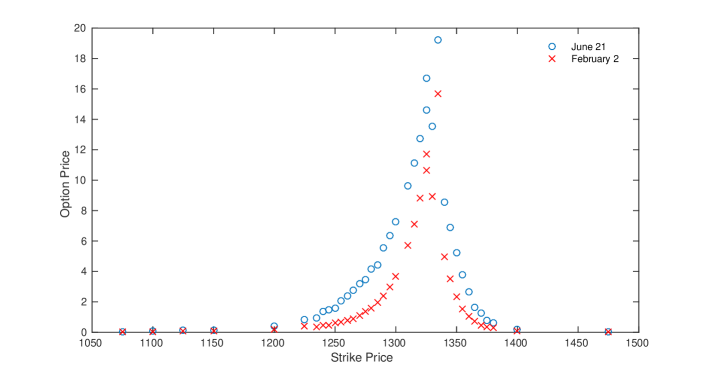
5 Empirical analysis

In this section we compare the empirical performance of the estimators introduced above. The Variance-Gamma estimator, being a simple yet non-trivial parametric approach, can be considered as a benchmark.

The analysis is carried out on the full data set as well as on a trimmed data set, where options with price lower than 1/8 or implied volatility higher than 0.7 are discarded a priori (the latter preliminary screening follows the approach of [1]). Moreover, we consider both put and call options, that is, in one case we discard a priori all call prices, and in another case all put prices. We have hence four different data sets on which the (daily) performance of the estimators is tested.

We are going to perform out-of-sample tests as follows: let $(p_{k})_{k\in J_{t}}$ be observed put option prices in a fixed trading day $t$, with $J_{t}=J_{t}^{0}\cup J_{t}^{1}$, $J_{t}^{0}\cap J_{t}^{1}=\varnothing$. The index set $J_{t}^{0}$ is used to construct estimators of option prices and is randomly chosen such that its size is 90% (up to rounding to the next integer) of the size of $J_{t}$. Since $t$ is fixed, under the hypotheses of Section 3 we can write, without loss of generality, $p_{k}=\pi_{p}(K_{k},T_{k}-t)$ for all $k\in J_{t}$. Denoting any of the estimators of Section 3 by $\hat{\pi}$, constructed on the basis of $(p_{k},K_{k},T_{k}-t)_{k\in J_{t}^{0}}$, we obtain estimates $\hat{p}_{k}=\hat{\pi}(K_{k},T_{k}-t)$ for all $k\in J_{t}^{1}$. These estimates are well defined, or meaningful, only for those $k\in J_{t}^{1}$ such that $(K_{k},T_{k}-t)$ belongs to the convex hull of $(K_{k},T_{k}-t)_{k\in J_{t}^{0}}$ whenever a linear estimator or a Nadaraya-Watson estimator is used. The (relative) error for any one of the estimators is then simply defined as $e_{k}=\lvert 1-\hat{p}_{k}/p_{k}\rvert$ for all $k\in J_{t}^{1}$ such that $\hat{p}_{k}$ is well defined. This procedure is repeated for all trading days of the year. We the compute various averages and related statistics on the obtained sample of relative errors $(e_{k})_{k}$ for the whole year.

Remark 5.1.

Discarding all call prices to construct estimators of the pricing functional for put prices (and vice versa) implies that a large amount of potentially useful information is being discarded. In fact, in view of put-call parity, prices of call options can be translated into prices of put options with the same maturity and strike price, exactly as in the procedure described at length in Section 4. However, given the usual characteristics of call and put options on the S&P500, using the additional information does not improve essentially the accuracy of the estimators. In fact, as one can see in Figure 2, the set of points $(K,x)$ for call and put options, where $K$ and $x$ stand for strike price and time to maturity, respectively, are almost disjoint. It is clear, on the other hand, that taking into account the information contained in the whole set of option prices could be very useful to price (deep) ITM options.

Figure 2: Time to maturity and strike prices: call vs. put

This figure shows time to maturity and strike price of all options traded in one day (June 21, 2012).

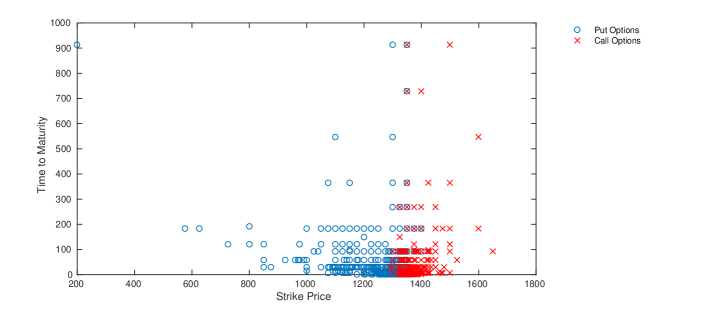
Before presenting the empirical results, let us briefly introduce the labels used below and in the corresponding tables:

LI

Normalized linear interpolator of the pricing function defined in §3.1.

BS

Black-Scholes price with volatility obtained by normalized linear interpolation of the volatility surface, as defined in §3.3.

NW

Nadaraya-Watson estimator of the pricing function with smoothing parameters chosen by a quantile-based criterion, as defined in §3.2.

NWCV

As NW, but with smoothing parameter chosen by cross-validation.

BS-NW

Black-Scholes price with volatility obtained by Nadaraya-Watson estimation.

BS-NWCV

As BS-NW, but with smoothing parameter chosen by cross-validation.

VG

The Variance-Gamma estimator as defined in §3.4.

5.1 Pricing within the hull

Statistics on the empirical pricing error computed on the whole data set, both for the case of put and of call options, are collected in Table 3. Since, as mentioned above, the linear interpolator of the pricing functional (LI) as well as the the linear interpolator of the implied volatility function (hence BS) are only defined on the convex hull of the sets of couples $(K_{k},T_{k}-t)_{k\in J_{t}^{0}}$, for all $t$, the set of empirical errors $(e_{k})_{k}$ is restricted to those $k$ such that the linear interpolator is well defined. This restriction implies that $5.1\%$ of the put options and $7.4\%$ of the call options (whose index $k$ belongs to $J_{t}^{1}$ for some $t$) cannot be priced by methods relying on linear interpolation. The behavior of the estimators that do not suffer of this restriction (at least formally) is discussed later.

It turns out that all non-parametric estimators, if evaluated in terms of their mean $L_{1}$ relative error, are not satisfactory, with figures ranging from around 9% to 40%. The parametric estimator based on the Variance-Gamma process (VG) has even higher mean errors.

Table 3: Pricing errors on the full dataset

The table displays descriptive statistics on the empirical pricing errors (in percentage points) of the various estimators, on the basis of the complete dataset. Some points of the empirical distribution of the pricing error are also reported. The labels used for the different estimators are defined on page 5. The sample period is January 3, 2012 to December 31, 2012. The pricing error is computed on 4460 put options and on 2732 call options.

Put Options
Error	LI	BS	NW	BS-NW	NWCV	BS-NWCV	VG
Mean	11.9	10.7	289.1	39.8	29.5	32.2	46.9
St. Dev.	49.0	130.8	985.7	249.4	113.2	280.5	28.0
Median	3.1	1.1	26.9	16.0	10.8	6.4	45.7
Min	0.0	0.0	0.0	0.0	0.0	0.0	0.0
Max	2027.0	8079.8	17792.1	15551.7	4649.3	16892.0	314.7
Empirical Distribution
$1\%$	23.7	48.0	3.1	6.2	8.1	16.3	0.9
$5\%$	61.6	73.4	13.4	25.8	30.2	44.2	4.6
$10\%$	75.9	82.9	24.5	40.0	47.4	60.0	9.3
$20\%$	87.5	91.2	41.6	55.0	69.8	73.6	18.9
$25\%$	90.0	93.0	48.0	59.6	75.7	77.0	23.9
$30\%$	92.2	94.6	52.6	63.5	80.2	79.9	29.3
$50\%$	96.0	97.2	65.3	75.4	89.3	87.0	56.6
Call Options
Error	LI	BS	NW	BS-NW	NWCV	BS-NWCV	VG
Mean	30.1	8.7	278.3	26.6	40.0	14.7	57.4
St. Dev.	418.0	36.6	1013.1	48.1	180.0	51.1	30.3
Median	5.0	1.3	29.2	7.9	15.6	4.2	64.8
Min	0.0	0.0	0.0	0.0	0.0	0.0	0.0
Max	16075.0	1125.9	16053.6	830.2	4733.0	1811.3	276.1
Empirical Distribution
$1\%$	18.9	45.8	2.4	10.0	7.5	19.4	1.9
$5\%$	50.0	73.6	10.0	38.4	23.5	55.3	5.2
$10\%$	67.9	83.4	17.9	54.7	35.7	71.4	9.0
$20\%$	81.8	91.1	36.7	68.1	58.7	84.2	16.4
$25\%$	85.4	93.3	45.2	72.2	65.8	87.0	19.5
$30\%$	87.8	94.9	50.9	74.7	72.6	88.9	22.5
$50\%$	93.2	97.4	64.6	82.7	85.8	94.2	36.3

A more accurate evaluation of the performance of the estimators is obtained by looking at the distribution of the empirical errors, some points of which are also displayed in Table 3. In particular, one observes that the best performance, in terms of the number of options whose estimated price is reasonably near the market price, is achieved by the estimator based on Black-Scholes formula with linearly interpolated volatility (BS). It is also evident that the LI estimator has a considerably worse performance that the BS estimator. Similarly, the Nadaraya-Watson estimator of the pricing functional displays much weaker performance than the BS estimator, both when the smoothing parameter is chosen via a simple quantile-based criterion and when it is chosen via cross validation. In spite of the major improvement of the NW-based methods when cross validation is used with respect to their simpler quantile-based counterparts, all NW-based methods perform considerably worse than both methods based on simple linear interpolation, that is LI and BS. Taking into account that the choice of the smoothing parameter by cross validation is computationally much more intensive (and slower) than linear interpolation, these empirical results suggest that, for the purpose of the pricing problem treated here, keeping things simple is not only faster, but also significantly more accurate. At this point we should remark that the empirical results reported in this section are obviously influenced by the (random) splitting of the index set $J_{t}$ in two disjoint sets $J_{t}^{0}$ and $J_{t}^{1}$ for each date $t$. However, while changing the initialization of the random number generator (obviously) results in different figures, the qualitative observations just made, as well as the conclusions they imply, do not change.

The whole analysis has also been carried out on a smaller data set, obtained by eliminating those options whose implied volatility is higher than $70$% or price is lower than $$1/8$. This procedure is adopted in [1] and is repeated here only for comparison purposes with the results summarized in Table 3 (recall, however, that, as discussed above, the analysis of [1] and ours are not directly comparable). The corresponding results are collected in Table 4.

Table 4: Pricing errors on the trimmed dataset

The table displays descriptive statistics on the empirical pricing errors (in percentage points) of the various estimators, on the basis of the trimmed dataset. Some points of the empirical distribution of the pricing error are also reported. The labels used for the different estimators are defined on page 5. The sample period is January 3, 2012 to December 31, 2012. The pricing error is computed on 4021 put options and on 2496 call options.

Put Options
Error	LI	BS	NW	BS-NW	NWCV	BS-NWCV	VG
Mean	9.5	4.8	151.4	20.8	22.8	17.9	38.5
St. Dev.	35.5	13.3	425.5	29.0	62.6	72.8	24.6
Median	3.2	1.0	24.8	10.2	10.8	5.5	35.9
Min	0.0	0.0	0.0	0.0	0.0	0.0	0.0
Max	1129.3	322.9	6152.4	527.5	1462.2	3358.0	202.0
Empirical Distribution
$1\%$	21.7	50.1	3.1	10.0	8.6	17.7	1.2
$5\%$	62.0	78.6	13.2	33.6	31.1	48.1	5.8
$10\%$	79.6	88.0	25.0	49.6	48.0	64.3	12.0
$20\%$	91.3	95.1	43.0	67.0	71.1	78.6	25.2
$25\%$	93.6	96.4	50.2	73.0	78.3	82.3	31.9
$30\%$	94.6	97.1	55.7	77.4	83.0	85.2	40.0
$50\%$	97.6	98.7	68.9	87.6	91.6	91.9	72.5
Call Options
Error	LI	BS	NW	BS-NW	NWCV	BS-NWCV	VG
Mean	14.4	5.2	138.4	14.3	31.3	9.3	49.6
St. Dev.	45.2	18.7	375.1	20.0	77.0	17.6	27.6
Median	4.6	1.1	27.3	6.8	16.1	3.8	54.2
Min	0.0	0.0	0.0	0.0	0.0	0.0	0.0
Max	1233.6	649.1	4954.1	217.9	1952.5	315.4	227.0
Empirical Distribution
$1\%$	17.7	47.2	2.5	9.7	7.6	19.2	2.3
$5\%$	51.8	79.2	11.1	41.5	23.2	57.1	6.7
$10\%$	69.4	88.1	19.7	60.8	34.9	75.1	11.7
$20\%$	83.5	94.6	38.5	79.1	57.9	88.5	19.3
$25\%$	87.3	96.0	46.4	82.6	65.6	91.2	23.2
$30\%$	89.5	96.4	53.6	86.1	72.5	93.2	27.2
$50\%$	94.2	98.4	69.0	93.7	86.2	97.0	45.0

Even though, as is natural to expect, the mean pricing error improves for all estimators, the qualitative picture emerged from the analysis of the whole data set does not change. In particular, the only NW-based method with a barely acceptable performance is the Black-Scholes estimator coupled with estimation of the implied volatility when the smoothing parameter is chosen by cross validation. The important qualitative observation, though, is, as before, that keeping things simple, especially using the BS estimator, is both faster and more accurate in the vast majority of cases. Another important qualitative conclusion is that pricing by non-trivial fully parametric models, such as the Variance-Gamma model of §3.4 , calibrated to observed option prices, does not produce reliable estimates, even though the model allows for skewed and (moderately) heavy-tailed distributions of returns.

The empirical distribution of the (absolute) pricing errors clearly indicates that the mean errors are heavily influenced by relatively few large values. This observation holds both for the whole as well as for the reduced dataset. For instance, the mean pricing error of the LI method for put options is around $12$% and $9.5$%, respectively, while more than $75$% of the errors are less than $10$% in both cases. In particular, by direct inspection of the results obtained for a few randomly chosen dates, one observes that high relative errors mostly afflict options with low prices. It appears therefore interesting to analyze the pricing performance of the various estimators on “expensive” options, i.e. whose (observed, not estimated) price is higher than $1\$$, respectively.

Table 5: Pricing errors on options with price larger than $\$1$ (full dataset)

The table displays descriptive statistics on the empirical pricing errors (in percentage points) of the various estimators restricted to options in the full dataset whose price is larger than $\$1$. Some points of the empirical distribution of the pricing error are also reported. The labels used for the different estimators are defined on page 5. The sample period is January 3, 2012 to December 31, 2012. The pricing error is computed on 3222 put options and on 2137 call options.

Put Options
Error	LI	BS	NW	BS-NW	NWCV	BS-NWCV	VG
Mean	7.4	2.4	37.9	20.4	17.8	12.3	47.7
St. Dev.	31.0	7.4	71.2	35.8	57.4	33.9	24.1
Median	2.4	0.6	17.6	9.0	9.1	4.0	47.2
Min	0.0	0.0	0.0	0.0	0.0	0.0	0.0
Max	777.4	158.0	894.7	1051.8	2170.1	722.8	100.0
Empirical Distribution
$1\%$	25.8	60.7	3.8	8.3	7.7	21.1	0.7
$5\%$	73.2	88.6	17.6	34.5	34.0	56.0	3.6
$10\%$	86.8	95.6	32.5	52.8	53.4	73.6	7.2
$20\%$	94.2	98.6	54.7	70.6	77.6	86.0	15.0
$25\%$	95.5	98.9	62.9	75.5	83.2	88.9	19.4
$30\%$	96.6	99.1	68.8	79.6	87.4	91.1	24.4
$50\%$	98.0	99.6	84.2	90.0	94.4	95.3	54.2
Call Options
Error	LI	BS	NW	BS-NW	NWCV	BS-NWCV	VG
Mean	12.7	3.4	43.4	13.6	25.1	6.8	61.6
St. Dev.	51.5	13.3	100.5	23.3	63.8	14.0	26.4
Median	3.6	0.8	21.6	5.4	14.2	3.0	71.1
Min	0.0	0.0	0.0	0.0	0.0	0.0	0.0
Max	1287.4	270.5	3414.3	355.6	1437.5	273.0	98.9
Empirical Distribution
$1\%$	20.7	55.8	3.1	12.4	7.5	23.6	1.9
$5\%$	58.4	85.8	12.5	47.5	25.4	65.9	4.7
$10\%$	77.3	93.8	22.4	67.4	38.9	83.1	7.4
$20\%$	88.3	97.3	46.4	81.5	63.9	93.4	12.4
$25\%$	90.7	98.2	57.0	85.7	71.3	95.2	14.5
$30\%$	92.0	98.7	63.9	87.8	78.1	96.4	16.6
$50\%$	95.7	99.3	80.4	93.6	90.6	98.6	27.5

The corresponding results are reported in Tables 5: the BS estimator still exhibits a quite strong performance with mean absolute error around $2$ - $3$% and more than $85$% of options priced within a $5$% error margin. On the other hand, other estimators show a somewhat inconsistent performance: the LI estimator for put options has a mean price error of approximately $7$%, which increases to over $12$% for call options, while a completely symmetrical behavior is displayed by the BS-NW estimator. The main qualitative conclusions drawn above are confirmed also in this situation: among the NW-based methods, only the BS-NWCV is in some cases acceptable, and the simple linear interpolation-based BS estimator still outperforms (by far) all others.

Moreover, a comparison of the cumulative distribution functions of (the absolute value of) the relative pricing error reveals that the BS estimator stochastically dominates all other estimators (see Figure 3). This conclusion is also supported by the results of a two-sample Kolmogorov-Smirnov test, which rejects the hypothesis at confidence level 5% that the errors of any two estimators may come from the same distribution.

Figure 3: Cumulative distribution functions of pricing errors

This figure shows the cumulative distribution functions of pricing errors of the various estimators, on the basis of the complete dataset. The labels used for the different estimators are defined on page 26. The sample period is January 3, 2012 to December 31, 2012. The pricing error is computed on 2732 call options (Panel A) and on 4460 put options (Panel B).

Panel A	Panel B

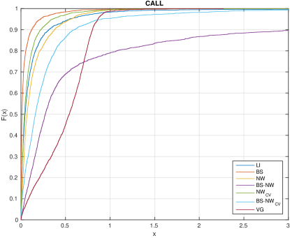
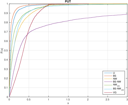
5.2 Pricing outside the hull

As seen above, the NW-based as well as the VG estimators can (in principle) estimate the prices at time $t$ of options whose parameters $K$ and $T-t$ do not fall within the convex hull of $(K_{k},T_{k}-t)_{k\in J^{0}_{t}}$. Let us recall, however, that NW non-parametric regression simply produces estimates that are weighted averages, hence, as already remarked in §3.2, estimates for parameters falling outside the convex hull of $J^{0}_{t}$ should be taken with extreme care. Results on the empirical pricing error relative to options whose parameters fall outside the convex hull of $J_{t}^{0}$, $t=1,\ldots,250$, are reported in Tables 6 and 7: with mean errors over $30$% and $50$% or more options mispriced by at least $20$%, the BS-NWCV estimator, which also in this case performs better than all other NW-based as well as VG estimators, could at best be used to get rough estimates of the correct price.

Table 6: Pricing errors outside the convex hull (full dataset)

The table displays descriptive statistics on the empirical pricing errors (in percentage points) of the various estimators restricted to those options for which the LI estimator is not defined, on the basis of the full dataset. Some points of the empirical distribution of the pricing error are also reported. The labels used for the different estimators are defined on page 5. The sample period is January 3, 2012 to December 31, 2012. The pricing error is computed on 241 put options and on 217 call options.

Put Options
Error	NW	BS-NW	NWCV	BS-NWCV	VG
Mean	996.3	50.7	1945.7	49.8	62.9
St. Dev.	3381.5	45.5	10228.9	49.3	45.1
Median	69.0	45.5	66.5	38.7	50.8
Min	0.0	0.0	0.0	0.0	0.0
Max	44100.0	253.4	128466.9	380.6	271.1
Empirical Distribution
$1\%$	3.7	7.5	8.7	8.7	0.8
$5\%$	6.2	19.9	10.8	24.9	4.1
$10\%$	7.1	34.4	13.3	37.8	13.7
$20\%$	14.1	41.1	22.4	44.4	22.0
$25\%$	18.7	44.4	27.4	45.6	24.1
$30\%$	22.4	46.1	30.7	48.1	29.5
$50\%$	33.2	51.0	41.9	52.3	49.8
Call Options
Error	NW	BS-NW	NWCV	BS-NWCV	VG
Mean	1527.5	39.9	2110.3	36.4	53.6
St. Dev.	8394.3	47.6	13801.4	45.7	57.2
Median	62.2	11.2	63.6	15.5	47.7
Min	0.3	0.0	0.0	0.0	0.0
Max	107881.1	278.1	153605.4	278.1	342.5
Empirical Distribution
$1\%$	2.3	19.4	6.5	20.3	18.4
$5\%$	7.4	39.6	10.1	40.1	23.0
$10\%$	15.2	48.8	16.1	46.1	29.5
$20\%$	27.6	55.3	25.3	53.9	37.3
$25\%$	33.6	57.1	29.0	55.3	40.6
$30\%$	35.9	59.0	34.1	59.0	43.8
$50\%$	43.8	63.1	42.4	67.7	51.6

Table 7: Pricing errors outside the convex hull (trimmed dataset)

The table displays descriptive statistics on the empirical pricing errors (in percentage points) of the various estimators restricted to those options for which the LI estimator is not defined, on the basis of the trimmed dataset. Some points of the empirical distribution of the pricing error are also reported. The labels used for the different estimators are defined on page 5. The sample period is January 3, 2012 to December 31, 2012. The pricing error is computed on 251 put options and on 225 call options.

Put Options
Error	NW	BS-NW	NWCV	BS-NWCV	VG
Mean	682.9	51.5	414.5	46.1	58.0
St. Dev.	1404.9	39.6	1617.0	38.9	48.3
Median	120.8	59.3	40.5	44.8	43.6
Min	0.0	0.0	0.0	0.0	0.1
Max	9526.7	232.1	15964.3	232.1	316.5
Empirical Distribution
$1\%$	0.8	5.2	6.4	8.0	1.2
$5\%$	1.6	17.9	9.6	24.3	7.6
$10\%$	5.2	27.1	13.9	30.3	15.1
$20\%$	11.2	35.5	23.1	38.6	23.9
$25\%$	13.5	37.5	29.9	40.6	26.7
$30\%$	15.5	39.8	34.7	42.2	32.7
$50\%$	33.1	45.4	57.4	52.6	55.8
Call Options
Error	NW	BS-NW	NWCV	BS-NWCV	VG
Mean	650.2	34.3	321.7	32.8	46.3
St. Dev.	1357.2	42.8	897.7	45.0	45.1
Median	77.9	15.3	66.7	16.2	38.0
Min	0.2	0.0	0.0	0.0	0.0
Max	7997.1	277.8	6147.3	280.4	213.2
Empirical Distribution
$1\%$	1.8	19.6	4.4	20.0	20.0
$5\%$	4.4	34.2	7.6	36.4	25.3
$10\%$	9.3	44.4	10.7	43.1	31.1
$20\%$	21.8	54.2	21.8	51.1	37.8
$25\%$	25.8	56.9	29.8	56.9	41.3
$30\%$	30.7	59.6	34.7	61.3	44.4
$50\%$	43.6	69.3	44.4	75.6	59.1

A way to extend the domain of definition of estimators based on linear interpolation is to augment $J_{t}^{0}$, for each $t$, with a set of fictitious parameters and corresponding option prices. In particular, one can add synthetic options with time to maturity equal to $0$, so their prices are equal to their payoff. For each $t$, augmenting $J_{t}^{0}$ with $30$ couples of the type $(K_{k},0)_{k=1,\ldots,30}$, where $(K_{k})$ are increasing, equally spaced, ranging between the smallest and the largest strike price of all options in $J^{t}$, we obtain an “augmented” LI estimator. This enlarges the domain of definition of LI, so that the proportion of options that cannot be prices drops to $2$% for put options and to $3.3$% for call options. The extension procedure just described can be applied to any data set, as the fictitious prices are universal. However, since observed prices tend to be higher than theoretical prices for small times, it does not seem reasonable to eliminate from the data set options with low price, which in the large majority of cases also have very short time to maturity, and then to artificially add options with time to maturity equal to zero. In other words, the extension procedure should be applied only, if necessary, to the full data set, and this is what we do. The empirical results are reported in Table 8.

Table 8: Linear estimator with fictitious options

The table displays descriptive statistics on the empirical pricing errors (in percentage points) of the “augmented” normalized linear estimator, defined in §5.2 and labeled LIB, on the basis of the full dataset. For comparison, the first column reports the statistics for the normalized linear interpolator (LI). The sample period is 01/03/2012 to 12/31/2012.

	Put Options		Call Options
Error	LI	LIB	LI	LIB
Mean	11.9	14.0	30.1	30.4
St. Dev.	49.0	47.5	418.0	211.6
Median	3.1	3.5	5.0	5.3
Min	0.0	0.0	0.0	0.0
Max	2027.0	1167.4	16075.0	8860.8
Priced options	4460	4607	2732	2851

Appendix A Appendix

A.1 Sensitivity of implied volatility against dividend

We place ourselves in the well-known Black-Scholes setting. Let us denote by $C$ the price of a European call option on a dividend-paying stock, so that

$$C=Se^{-qt}\Phi(d_{+})-Ke^{-rt}\Phi(d_{-}),$$

where

$$d_{+}:=\frac{\log S/K+\bigl{(}r-q+\sigma^{2}/2\bigr{)}t}{\sigma\sqrt{t}},\qquad d_{-}:=d_{+}-\sigma\sqrt{t}.$$

Recalling that

$$Se^{-qt}\phi(d_{+})=Ke^{-rt}\phi(d_{-}),$$ (4)

it is immediate to obtain

$$\frac{\partial C}{\partial q}=-tSe^{-qt}\Phi(d_{+}).$$

Moreover, one has

$$\frac{\partial C}{\partial\sigma}=\sqrt{t}Se^{-qt}\phi(d_{+}).$$

In particular, denoting the function $(q,\sigma)\mapsto C$ again just by $C$ (i.e. treating all other parameters as constants), the implicit function theorem implies that, for any $q_{0}$, $\sigma_{0}$, there exists a function $\varsigma:\mathbb{R}_{+}\to\mathbb{R}_{+}$ (to be interpreted as implied volatility) such that $\sigma_{0}=\varsigma(q_{0})$, $C=C(q,\varsigma(q))$, and

$$\frac{\partial\varsigma}{\partial q}(q_{0})=-\frac{\partial C}{\partial q}(q_{0},\sigma_{0})\,\frac{\partial C}{\partial\sigma}(q_{0},\sigma_{0})=\sqrt{t}\frac{\Phi(d_{+})}{\phi(d_{+})},$$

where $d_{\pm}=d_{\pm}(q_{0},\sigma_{0})$. For the reader’s convenience, we are going to prove (4), which is obviously equivalent to

$$\frac{S}{K}e^{(r-q)t}=\frac{\phi(d_{-})}{\phi(d_{+})}=\exp\Bigl{(}\bigl{(}d_{-}^{2}-d_{+}^{2}\bigr{)}/2\Bigr{)},$$

hence also to

$$\log(S/K)+(r-q)t=\frac{d_{-}^{2}-d_{+}^{2}}{2}=\frac{1}{2}(d_{-}-d_{+})(d_{-}+d_{+}).$$

This identity can be verified by a direct computation, thus showing the validity of (4).

References

- [1] Y. Ait-Sahalia and A. W. Lo, Nonparametric Estimation of State-Price Densities Implicit in Financial Asset Prices, Journal of Finance 53 (1998), no. 2, 499–547.
- [2] Brendan K. Beare and Lawrence Schmidt, An empirical test of pricing kernel monotonicity, Journal of Applied Econometrics 31 (2016), no. 2, 338–356.
- [3] H. J. Bierens, Kernel estimators of regression functions, Advances in Econometrics (T. F. Bewley, ed.), Cambridge University Press, 1987, pp. 99–144.
- [4] P. Carr, H. Geman, D. B. Madan, and M. Yor, Stochastic volatility for Lévy processes, Mathematical Finance 13 (2003), no. 3, 345–382. MR 1995283 (2005a:91054)
- [5] P. Carr and L. Wu, Finite Moment Log Stable Process and Option Pricing, Journal of Finance 58 (2003), no. 2, 753–777.
- [6] M. Chernov and E. Ghysels, A study towards a unified approach to the joint estimation of objective and risk neutral measures for the purpose of options valuation, Journal of Financial Economics 56 (2000), no. 3, 407 – 458.
- [7] M. Grith, W. K. Härdle, and M. Schienle, Nonparametric estimation of risk-neutral densities, Handbook of computational finance, Springer Handb. Comput. Stat., Springer, Heidelberg, 2012, pp. 277–305. MR 2908476
- [8] Jens Carsten Jackwerth and Mark Rubinstein, Recovering probability distributions from option prices, The Journal of Finance 51 (1996), no. 5, 1611–1631.
- [9] O. Kallenberg, Foundations of modern probability, second ed., Springer-Verlag, New York, 2002. MR 1876169 (2002m:60002)
- [10] I. Karatzas and S. E. Shreve, Methods of mathematical finance, Springer-Verlag, New York, 1998. MR MR1640352 (2000e:91076)
- [11] D. B. Madan, P. Carr, and E. C. Chang, The Variance Gamma Process and Option Pricing., European Finance Review 2 (1998), 79–105.
- [12] E. A. Nadaraya, On Estimating Regression, Theory of Probability and Its Applications 9 (1964), no. 1, 141–142.
- [13] F. P. Preparata and M. I. Shamos, Computational geometry, Springer-Verlag, New York, 1985. MR 805539
- [14] J. V. Rosenberg and R. F. Engle, Empirical pricing kernels, Journal of Financial Economics 64 (2002), no. 3, 341 – 372.
- [15] K. Sato, Lévy processes and infinitely divisible distributions, Cambridge University Press, Cambridge, 1999. MR MR1739520 (2003b:60064)
- [16] B. W. Silverman, Density estimation for statistics and data analysis, Chapman & Hall, London, 1986. MR 848134 (87k:62074)
- [17] A. B. Tsybakov, Introduction to nonparametric estimation, Springer, New York, 2009. MR 2724359 (2011g:62006)
- [18] G. S. Watson, Smooth regression analysis, Sankhyā: The Indian Journal of Statistics. Series A 26 (1964), 359–372.