Topological quantum phase transition of light

Abstract

We study theoretically the topological quantum phase transition in Cavity QED lattice. We predict the condition for non-topological phase to the topological phase transition conditions for three different model Hamiltonians in cavity QED lattice. We study these topological quantum phase transition through winding number, which is a topological invariant quantity. We argue that the appearance of topological phase in these systems where the discrete $Z_{2}$ symmetry broken. We show that the non-topological state is the vacuum state of the system where each cavity contains fermionic type excitations from light-matter interaction whereas the topological state of system contains Majorana modes of excitations at the end cavity of the lattice.

Keywords: Topological Quantum Phase Transition , Quantum Optics

I I. Introduction

In condensed matter system, quantum phase transition plays a significant role to study and explain different quantum phases of the system which explain the different broken symmetry states of the system, which are used to describe with the concept of local order parameter of Ginzburg-Landau Theory berni ; ss .
The major limitation of Ginzburg-Landau theory is that the order parameter is treated as a local order parameter, this is over come by Topological quantum phase transition berni . In recent years, it reveals experimentally and theoretically in condensed matter system that the typical order parameter is not a local order parameter rather it is highly non-local order parameter berni . One of the example for the non local order parameter is quantum Hall state which corresponds to the annihilating an electron at a position by unwinding the number of fluxes. This flux unwinding process is highly non-local and Ginzburg-Landau theory is not able to describe this phenomena. The states with non-local order parameter are termed topologically ordered. The fact that topology is a characterization of global shape and it is invariant under a small local deformation it becomes one of the important property of the system [1]. This topological robustness protects the quantum state from the external perturbation. As a consequence of it several interesting physical phenomena appears in the low dimensional quantum many body system berni ; nayak .
As the physics of spontaneous symmetry breaking is absent for the topological state of matter, the concept of order parameter is also absent to explain the relevant low energy physics of these systems. The topological phases are characterized by topological invariants integer number. In the present research problem, we do the explicit study of the topological quantum phase transition through winding number study.
Motivation:
The study of topological phases of quantum many body systems are still in the beginning phase. Therefore to search the topological states in different physical system is increasing rapidly. The topological phases of condensed matter system attract much more attention due to their practical application in low dimensional quantum many body system [1,3]. Here we state few examples of topological states of matter in condensed matter physics.
Integer quantum Hall effect, fractional quantum Hall effect, quantum spin Hall effect, topological insulator. But the topological state of matter for cavity QED has not explored yet to the mark horo ; agarwal .
The other part of the motivation comes from the Kitaev’s seminal paper kitaev . Kitaev has proposed the model of one dimensional spinless p-wave superconductors to realize the existence of topological phase. At that period, it is difficult to realize Kitaev’s model in reality. The electron carry spin-1/2, the first step is to freeze the spin of the particle so that the system appears as a one dimensional spinless system. In the interacting light-matter system, specially in the cavity QED system where the experimental advancement is in the state of art and the spin of the system mimics the state level difference and the measurement of quantum state is extremely precise horo ; agarwal . In low-dimensional interacting light-matter system excitations appear as a collective mode under certain physical conditions it behaves as a Majorana fermion mode sujop . Therefore we decide to explain the topological state of interacting light-matter system and also to realize the Kitaev’s model for cavity QED system.

II II. The Model Hamiltonians and The Derivation of Effective Hamiltonians

The Hamiltonian of our present study consists of three parts:

$$H~{}=~{}{H_{A}}~{}+~{}{H_{C}}~{}+~{}{H_{AC}}$$ (1)

The Hamiltonians are the following

$${H_{A}}~{}=~{}\sum_{j=1}^{N}{{\omega}_{e}}|e_{j}><e_{j}|~{}+~{}{\omega}_{ab}|b_{j}><b_{j}|,$$ (2)

where $j$ is the cavity index. ${\omega}_{ab}$ and ${\omega}_{e}$ are the energies of the state $|b>$ and the excited state respectively. The energy level of state $|a>$ is set as zero. $|a>$ and $|b>$ are the two stable state of a atom in the cavity and $|e>$ is the excited state of that atom in the same cavity. The following Hamiltonian describes the photons in the cavity,

$${H_{C}}~{}=~{}{{\omega}_{C}}\sum_{j=1}^{N}{{a_{j}}}^{\dagger}{a_{j}}~{}+~{}{J_{C}}\sum_{j=1}^{N}({{a_{j}}}^{\dagger}{a_{j+1}}+h.c),$$ (3)

where ${a_{j}}^{\dagger}({a_{j}})$ is the photon creation (annihilation) operator for the photon field in the $j$’th cavity, ${\omega}_{C}$ is the energy of photons and $J_{C}$ is the tunneling rate of photons between neighboring cavities. The interaction between the atoms and photons and also by the driving lasers are described by

$${H_{AC}}~{}=~{}\sum_{j=1}^{N}[(\frac{{\Omega}_{a}}{2}e^{-i{{\omega}_{a}}t}+{g_{a}}{a_{j}})|e_{j}><a_{j}|+h.c]+[a\leftrightarrow b].$$ (4)

Here ${g_{a}}$ and ${g_{b}}$ are the couplings of the cavity mode for the transition from the energy states $|a>$ and $|b>$ to the excited state. ${\Omega}_{a}$ and ${\Omega}_{b}$ are the Rabi frequencies of the lasers with frequencies ${\omega}_{a}$ and ${\omega}_{b}$ respectively.
The authors of Ref. hart1 have derived an effective spin model by considering the following physical processes: A virtual process regarding emission and absorption of photons between the two stable states of neighboring cavity yields the resulting effective Hamiltonian as

$${H_{xy}}=\sum_{j=1}^{N}B{{\sigma}_{j}}^{z}~{}+~{}\sum_{j=1}^{N}(\frac{J_{1}}{2}{{\sigma}_{j}}^{+}{{\sigma}_{j+1}}^{-}~{}+~{}\frac{J_{2}}{2}{{\sigma}_{j}}^{-}{{\sigma}_{j+1}}^{-}+h.c).$$ (5)

When $J_{2}$ is real then this Hamiltonian reduces to the XY model. Where ${{\sigma}_{j}}^{z}=|b_{j}><b_{j}|~{}-~{}|a_{j}><a_{j}|$, ${{\sigma}_{j}}^{+}=|b_{j}><a_{j}|$, ${{\sigma}_{j}}^{-}=|a_{j}><b_{j}|$ .

$$H_{xy} = \sum_{i=1}^{N}(B{{\sigma}_{i}}^{z}~{}+~{}{J_{1}}({{\sigma}_{i}}^{x}{{\sigma}_{i+1}}^{x}+{{\sigma}_{i}}^{y}{{\sigma}_{i+1}}^{y})$$ (6)

$$+{J_{2}}({{\sigma}_{i}}^{x}{{\sigma}_{i+1}}^{x}-{{\sigma}_{i}}^{y}{{\sigma}_{i+1}}^{y}))$$

$$=\sum_{i=1}^{N}B({{\sigma}_{i}}^{z}~{}+~{}{J_{x}}{{\sigma}_{i}}^{x}{{\sigma}_{i+1}}^{x}~{}+~{}{J_{y}}{{\sigma}_{i}}^{y}{{\sigma}_{i+1}}^{y}).$$

With ${J_{x}}=(J_{1}+J_{2})$ and ${J_{y}}=(J_{1}-J_{2})$.
We follow the references hart1 , to present the analytical expression for the different physical parameters of the system.

$$B=\frac{\delta_{1}}{2}-\beta$$ (7)

$${J_{1}}=\frac{\gamma_{2}}{4}(\frac{{|{\Omega_{a}}|}^{2}{g_{b}}^{2}}{{{\Delta}_{a}}^{2}}+\frac{{|{\Omega_{b}}|}^{2}{g_{a}}^{2}}{{{\Delta}_{b}}^{2}}),{J_{2}}=\frac{\gamma_{2}}{2}(\frac{{\Omega_{a}}{\Omega_{b}}g_{a}g_{b}}{{\Delta}_{a}{\Delta_{b}}}).$$ (8)

The detail analytical expression for ${\gamma}_{ab},{\gamma}_{1},{\gamma}_{2},{\delta}_{1},{\Delta}_{a},{\Delta}_{b},{\delta_{a}}^{k},{\delta_{b}}^{k}$ and $\Omega_{k}$ are relegated to the appendix.
Here we discuss very briefly about an effective $z$-component of interactions (${{\sigma}_{i}}^{z}{{\sigma}_{i+1}}^{z}$) in such a system. The authors of Ref.hart1 ; hart2 have proposed the same atomic level configuration but having only one laser of frequency ${\omega}$ that mediates the atom-atom coupling through virtual photons. Another laser field with frequency $\nu$ is used to tune the effective magnetic field. In this case the Hamiltonian ${H_{AC}}$ changes but the Hamiltonians $H_{A}$ and $H_{C}$ are the same.

$${H_{AC}} = \sum_{j=1}^{N}[(\frac{{\Omega}}{2}e^{-i{{\omega}}t}+\frac{{\Lambda}}{2}e^{-i{{\nu}_{a}}t}{g_{a}}{a_{j}})|e_{j}><a_{j}|+h.c]$$ (9)

$$+[a\leftrightarrow b].$$

Here, ${\Omega}_{a}$ and ${\Omega}_{b}$ are the Rabi frequencies of the driving laser with frequency ${\omega}$ on transition $|a>\rightarrow|e>$ , $|b>\rightarrow|e>$, whereas ${\Lambda}_{a}$ and ${\Lambda}_{b}$ are the driving laser with frequency ${\nu}$ on transition $|a>\rightarrow|e>$ , $|b>\rightarrow|e>$. One can eliminate adiabatically the excited atomic levels and photons by considering the interaction picture with respect to $H_{0}=H_{A}~{}+~{}H_{C}$ [6,7]. They have considered the detuning parameter in such a way that the Raman transitions between two level are suppressed and also chosen the parameter in such a way that the dominant two-photon processes are thus no transition between levels a and b. Whenever two atoms exchange a virtual photon both of them experience a Stark shift and play the role of an effective ${{\sigma}^{z}}{{\sigma}^{z}}$ interaction hart1 ; hart2 . Then the effective Hamiltonian reduces to

$${H_{zz}}~{}=~{}\sum_{j=1}^{N}({B_{z}}{{\sigma}_{j}}^{z}~{}+~{}{J_{z}}{{\sigma}_{j}}^{z}{{\sigma}_{j+1}}^{z}).$$ (10)

These two parameters can be tuned independently by varying the laser frequencies. Finally, they have obtained an effective model by combining Hamiltonians $H_{xy}$ and $H_{zz}$ by using Suzuki-Trotter formalism hart1 ; hart2 . The effective Hamiltonian simulated by this procedure is

$$H_{spin}~{}=~{}\sum_{j=1}^{N}(B_{tot}{{\sigma}_{j}}^{z}~{}+~{}\sum_{{\alpha}=x,y,z}J_{\alpha}{{\sigma}_{j}}^{\alpha}{{\sigma}_{j+1}}^{\alpha}),$$ (11)

where $B_{tot}=B+{B_{z}}$. It has been shown in Ref. hart2 that $J_{y}$ is less than $J_{x}$. From the analytical expressions of $J_{x}$ and $J_{y}$, it is clear that the magnitudes of ${J_{1}}$ and $J_{2}$ are different. ${J_{z}}={\gamma}_{2}{|\frac{{{\Omega}_{b}}^{*}g_{b}}{4\Delta_{b}}-\frac{{{\Omega}_{a}}^{*}g_{a}}{4\Delta_{a}}|}^{2}$.
$B_{tot}=-\frac{1}{2}[\frac{{|{\Lambda}_{b}|}^{2}}{16{\tilde{\Delta_{b}}}^{2}}(4\tilde{\Delta_{b}}-\frac{{|{\Lambda_{a}}|}^{2}}{4({\tilde{\Delta}_{a}}-{\tilde{\Delta}_{b}})}-\frac{{|{\Lambda_{b}}|}^{2}}{{\tilde{\Delta}_{b}}}-{\beta_{2}})-{\beta_{3}}].$
The quantum state engineering of cavity QED is in the state of art due to the rapid progress of technological development of this field [3,4]. Therefore one can achieve this limit to get the desire Hamiltonian and quantum state of the system, when we consider the situation where $J_{y}=0$ and $J_{z}=0$. In this limit the atom-photon coupling strength $g_{a}=g_{b}$. The detail derivation is relegated to the appendix.
From the above equation, We get the following relations, $g_{b}=g_{a}$ to get the transverse Ising model. The detail derivation is relegated to the appendix.

$$H_{1}=\sum_{j=1}^{N}(B{{\sigma}_{z}}(j)+J_{x}{{\sigma}_{x}}(j){{\sigma}_{x}}(j+1)).$$ (12)

One can write the above Hamiltonian in spinless fermion operators by using the Jordan-Wigner transformation. To do so, we use the following relation.

$${\sigma_{n}}^{x}{\sigma_{n+1}}^{x} = ({{\psi}_{n}}^{\dagger}-{\psi_{n}})({{\psi}_{n+1}}^{\dagger}+{\psi_{n+1}})$$

$${\sigma_{n}}^{y}{\sigma_{n+1}}^{y} = ({{\psi}_{n}}^{\dagger}-{\psi_{n}})({{\psi}_{n+1}}^{\dagger}-{\psi_{n+1}})$$

$${\sigma_{n}}^{z}{\sigma_{n+1}}^{z} = (2{{\psi}_{n}}^{\dagger}{\psi_{n}}-1)(2{{\psi}_{n+1}}^{\dagger}{\psi_{n+1}}-1)$$ (13)

The Hamiltonian, $H_{1}$ become,

$$H_{1}=J_{x}\sum_{n}({\psi}^{\dagger}(n){\psi}(n+1)+h.c)+J_{x}\sum_{n}({\psi}^{\dagger}(n){\psi}^{\dagger}(n+1)+h.c)+2B\sum_{n}{\psi}^{\dagger}(n){\psi}(n).$$ (14)

We get this Hamiltonian for the condition $g_{a}=g_{b}$.
Similarly for the Hamiltonian, $H_{2}$, where $J_{x}$ and $J_{y}$ are non-zero. One can write the Hamiltonian in the following form.

$$H_{2}=(J_{x}+J_{y})\sum_{n}({\psi}^{\dagger}(n){\psi}(n+1)+h.c)+|J_{x}-J_{y}|\sum_{n}({\psi}^{\dagger}(n){\psi}^{\dagger}(n+1)+h.c)+2B\sum_{n}{\psi}^{\dagger}(n){\psi}(n).$$ (15)

We get this Hamiltonian for the condition, ${{\Omega}_{b}}^{*}g_{b}{\Delta}_{a}={{\Omega}_{a}}^{*}g_{a}{\Delta}_{b}$. The detail derivation is relegated to the appendix.
Similarly for the Hamiltonian, $H_{3}$, where $J_{x}$, $J_{y}$ and $J_{z}$ are non-zero.

$$H_{3}=(J_{x}+J_{y})\sum_{n}({\psi}^{\dagger}(n){\psi}(n+1)+h.c)+|J_{x}-J_{y}|\sum_{n}({\psi}^{\dagger}(n){\psi}^{\dagger}(n+1)+h.c)\\ +(2B+8\rho-4)\sum_{n}{\psi}^{\dagger}(n){\psi}(n).$$ (16)

where $\rho=<{{\psi}_{n}}^{\dagger}{\psi}_{n}>$ is the density of excitation in interacting light-matter system. Here we do the many body physics decoupling scheme to reduce the quartic interaction of the Hamiltonian to quadratic one.

$${\sigma_{n}}^{z}{\sigma_{n+1}}^{z}=(8\rho-4){\psi}^{\dagger}(n){\psi}(n)$$ (17)

After the Fourier transformation, the Hamiltonian, $H_{1}$ , reduce to,

$$H_{1} = 2\sum_{k>0}(2B+J_{x}cosk)({c_{k}}^{\dagger}{c_{k}}+{c_{-k}}^{\dagger}{c_{-k}})$$ (18)

$$+2iJ_{x}\sum_{k>0}sink({c_{k}}^{\dagger}{c_{-k}}^{\dagger}+{c_{k}}{c_{-k}}).$$

Similarly for the Hamiltonian, $H_{2}$ reduced to,

$$H_{2} = 2\sum_{k>0}(2B+(J_{x}+J_{y})cosk)({c_{k}}^{\dagger}{c_{k}}+{c_{-k}}^{\dagger}{c_{-k}})$$ (19)

$$+2i|J_{x}-J_{y}|\sum_{k>0}sink({c_{k}}^{\dagger}{c_{-k}}^{\dagger}+{c_{k}}{c_{-k}}).$$

Similarly the Hamiltonian, $H_{3}$ reduced to,

$$H_{3} = 2\sum_{k>0}((2B+8\rho-4)+(J_{x}+J_{y})cosk)({c_{k}}^{\dagger}{c_{k}}+{c_{-k}}^{\dagger}{c_{-k}})$$ (20)

$$+2i|J_{x}-J_{y}|\sum_{k>0}sink({c_{k}}^{\dagger}{c_{-k}}^{\dagger}+{c_{k}}{c_{-k}}).$$

Now our main interest is to study the topological quantum phase transition in cavity QED lattice system based on these models. Our starting point is to recast our three Hamiltonians ($H_{1},H_{2},H_{3}$) of interacting light-matter system.

$$H_{J=1,2,3}=[\sum_{n}-{t}^{J}({c_{n}}^{\dagger}c_{n+1}+h.c)-{\mu}^{J}{c_{n}}^{\dagger}{c_{n}}-{|\Delta|}^{J}({c_{n}}{c_{n+1}}+h.c)].$$ (21)

In the above Hamiltonian, we neglect the common negative sign which will not alter the relevant physics of the system.
${t}^{(1)}=J_{x}$, ${\Delta}^{(1)}=J_{x}$ and ${\mu}^{(1)}=2B$.
${t}^{(2)}=(J_{x}+J_{y})$, ${\Delta}^{(2)}=(J_{x}-J_{y})$ and ${\mu}^{(2)}=2B$.
${t}^{(3)}=(J_{x}+J_{y})$, ${\Delta}^{(3)}=(J_{x}-J_{y})$ and ${\mu}^{(2)}=2B+8\rho-4$.
The bulk properties of Hamiltonian can be studied in the momentum space. One can write down the Hamiltonian in momentum space as.

$$H^{k}_{J=1,2,3}=(\frac{1}{2})\sum_{k}{\psi_{k}}^{\dagger}{H^{k}_{J=1,2,3}}{\psi_{k}}$$ (22)

${H}_{J=1,2,3}=\left(\begin{array}[]{cc}{\epsilon}^{(J=1,2,3)}(k)&2{{\Delta}^{(J=1,2,3)}}^{*}(k)\\ 2{{\Delta}^{(J=1,2,3)}}(k)&-{\epsilon}^{(J=1,2,3)}\end{array}\right)$ where, ${\epsilon}^{(J=1,2,3)}=-2t^{(J=1,2,3)}cosk-{\mu}^{(J=1,2,3)}$, and ${\Delta^{(J=1,2,3)}}(k)=-i{\Delta}^{(J=1,2,3)}sink$.
This Hamiltonian corresponds to the p-wave superconducting phase, one can understand this in the following way.
One can also write down the above Hamiltonian in Bogoluibov energy spectrum,

$$H_{J=1,2,3}=\sum_{k}{E(k)}^{J}{a_{k}}^{\dagger}{a_{k}}$$ (23)

Here $E_{k}$ is the energy spectrum in bulk and ${a_{k}}^{\dagger}$ and $a_{k}$ are the Bogoliubov quasiparticles operators.

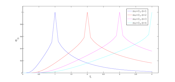
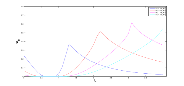
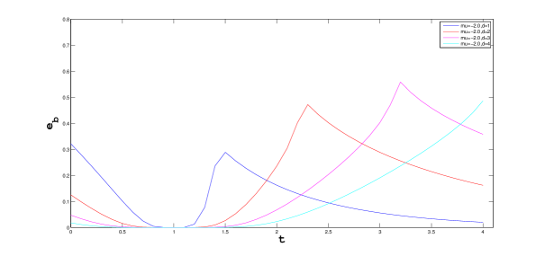
Figure 1: (Color online) Figures show the variation of $\epsilon_{b}$ with $t$ for different values $\Delta(=d=1,2,3,4)$. The upper panel is for the $\mu=0$, the middle one is for $\mu=-1.5$ and the lower one is for $\mu=-2$.

We express the model Hamiltonians of our system in terms of spinless p-wave superconducting Hamiltonian thus the starting point of our analysis is the seminal paper of Kitaev kitaev .
In the Majorana fermion basis Hamiltonian reduce to:

$$H^{J=1,2,3}=\left(\frac{-{\mu}^{J}}{2}\right)\sum\limits_{n=1}^{N}(1+i\gamma_{B,n}\gamma_{A,n})+\left(\frac{i}{2}\right)\sum\limits_{n=1}^{N-1}\left[({\Delta}^{J}+{t}^{J})\gamma_{B,n}\gamma_{A,n+1}+({\Delta}^{J}-{t}^{J})\gamma_{A,n}\gamma_{B,n+1}\right)$$

Here we use these analytical relations to derive the above Hamiltonian:
$c_{n}=\frac{1}{2}({\gamma}_{B,i}+{\gamma}_{A,i})$. ${{\gamma}_{B,i}}^{\dagger}={\gamma}_{B,i},{{\gamma}_{A,i}}^{\dagger}={\gamma}_{A,i}$. $\{\gamma_{\alpha,x},\gamma_{\beta,y}\}=2\delta_{\alpha,\beta}\delta_{x,y}$.
The index $A$ and $B$ are the arbitrary index. In the Kitaev’s chain if a Majorana fermion of $\gamma_{A}$ occurs at one end of the chain then the Majorana fermion $\gamma_{B}$ must occurs at the other end of the chain kitaev .
Now we discuss the non-topological states of the system. The first corresponds to $\mu<0$ but $t=\Delta=0$. From this condition, we analyze non-topological states of the three Hamiltonians.
For the Hamiltonian, $H_{1}$.
(1). $|{\Omega}_{a}|=0$ and $|{\Omega}_{b}|=0$, (2). $g_{b}=0,g_{a}=0$, (3). $|{\Omega}_{b}|=0,g_{a}=0$. (4). $|{\Omega}_{a}|=0,g_{b}=0$.
For the Hamiltonian, $H_{2}$, we obtain the same conditions to achieve the non-topological phase as we obtain in $H_{1}$. But the condition for $\mu$ is different for $H_{3}$. For $H_{1}$ and $H_{2}$, $\delta_{1}-2\beta<0$, but for $H_{3}$ the condition is $\delta_{1}-2\beta+8\rho-4<0$.
Physical explanation of the non-topological phase is the following:
The first term of the above Hamiltonian yields a coupling between the Majorana fermion modes in the same site. In the cavity QED system, this situation corresponds to the different kind of light-matter interactions which obeys that the coupled Majorana fermion modes condition in each cavity. It is well known that the two Majorana fermion modes produce a fermion mode. Thus the case of cavity QED system, the non-topological state of the system is the fermionic excitations. We consider this state as the vacuum state of the system where there is no gapless Majorana fermion excitation states. We consider this non-topological state as a vacuum state of the present system, actually it is the conventional superconducting phase.
Now our main intention is to find out the topological excitation which appears as a Majorana fermions. The condition for this phase is $\mu=0$ and $t=\Delta\neq 0$. Hence the Hamiltonian reduced to

$$H=-it\sum\limits_{n=1}^{N-1}\gamma_{B,n}\gamma_{A,n+1}.$$

It is very clear from the above Hamiltonian that ${\gamma_{1}}={\gamma_{A,1}}$ and ${\gamma}_{2}={\gamma}_{B,N}$ are not appear in the Hamiltonian. One can also write down the above Hamiltonian by introducing the new operator $B$.

$$B_{n}=\frac{1}{2}(\gamma_{A,n+1}+i\gamma_{B,n}).$$

$$H=t\sum\limits_{n=1}^{N-1}(B_{n}^{\dagger}B_{n}-1/2).$$

The ends of the chain has zero energy Majorana fermion modes $\gamma_{1}=\gamma_{A,1}$ and $\gamma_{2}=\gamma_{B,N}$. These can be considered as a non-local fermion $f=\frac{1}{2}(\gamma_{1}+i\gamma_{2})$. This fermion mode is in the zero energy configuration. In this topological phase, system is in the doubly degenerate ground state. One can understand this by following analysis.
If we consider $\left|0\right>$ is a ground state then $f\left|0\right>=0$ and $\left|{1}\right>=f^{\dagger}\left|0\right>$ is also a ground state with opposite fermion parity. The main difference between the conventional superconductor and topological superconductor is that the system has a unique ground state with an even parity such a way that all the electrons can form cooper pairs. Thus the conventional superconducting pairing is the vacuum state of the system. Therefore the non-topological state of the system is in the even parity state and the doubly degenerate ground state with opposite parity of the system is the topological state of the system.
Here we consider the most general situation, when $\mu\neq 0$ and $t\neq\Delta$. Here the main intuition is to study the transition for the topological state of the system to the non-topological state of the system.
In this arbitrary limit, the Majorana zero modes are no longer $\gamma_{A,1},\gamma_{B,N}$. In this limit wave function decay exponentially into the bulk of the system. The decay of this wave function results in the splitting of the degeneracy between the states $(f\left|0\right>=0,\left|1\right>=f^{\dagger}\left|0\right>)$. One can write down the effective Hamiltonian as

$$H_{eff}=\frac{i}{2}{e_{b}}b^{\prime}b^{\prime\prime}$$ (24)

when $e_{b}\propto e^{-\frac{L}{\xi_{0}}}$, $L$ is the length of the system. $b^{\prime}$ and $b^{\prime\prime}$ are the Majorana fermion at the left end and the right end of the chain respectively. $\xi_{0}^{-1}$ is the smallest of $|ln|\chi_{+}||$ and $|ln|\chi_{-}||$. When $\xi_{0}^{-1}$ is $0$ then the coherence length $\xi_{0}$ is $\infty$. At this point, the system transit from topological state to the non-topological state of the matter.

$$\chi_{\pm}=\frac{-\mu\pm\sqrt{\mu^{2}-4t^{2}+4|\Delta|^{2}}}{2(t+|\Delta|)}$$

$${{\xi}_{0}}^{-1}=Min[|ln|{\chi}_{+}||,|ln|{\chi}_{0}||]$$ (25)

$\epsilon\propto e^{-}\frac{L}{\xi_{0}}$ when $\xi_{0}^{-1}\Rightarrow 0$ then $e_{b}\propto 1$.
In fig. 1, we present the appearance of non-topological trivial state for different values of $\Delta(\Delta=1,2,3,4).$ It reveals from our study as we increase the value of $\Delta$, the non-topological phase occurs for the higher value of t. In the present situation the Majorana fermion modes decay exponentially into the bulk of the chain. The overlap of these wave function result in the splitting in the degeneracy between the state $\left|0\right>$ and $\left|1\right>$ by energy scale $e^{-\frac{L}{\xi}}$. This figures panel consist of three figures, it is clear from these study that as we go away from zero chemical potential to the higher one the peak at $t=\Delta$ of $e_{b}$ study gradually decreases. The coherence length $\xi\rightarrow\infty$ for only $\mu=0$, where the system shows the topological to non-topological transition. It is also clear from the analytical expression for $e_{b}$ that as we increase the length of the system keeping the other physical parameters of the system fixed, the system is in the stable topological state. Therefore it is clear from our study that the Majorana fermion modes appear at the edge is more stable for the array of larger length scale compare to the shorter one. Now we explain the corresponding physics in the light of cavity-QED lattice. In the topological phase, there is no bound between Majorana fermion mode between the two ends of the cavity. In the case of non-topological state, Majorana fermion mode excitation are now bound at the two end of the cavity. It is also clear from the above analysis of Kitaev’s formula kitaev that the that the transition from topological state to non-topological occurs only for $\mu=0$. ($t\neq 0\neq\Delta$). But we will also study the topological quantum phase transition through the variation of winding number calculation in the next section which yields more new and important result.

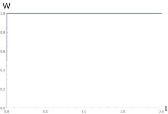
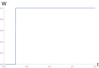
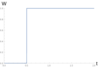
Figure 2: ( Color Online), Figures show the variation of winding number with t for different values of $\mu$. The upper panel is for the $\mu=0$, the middle panel is for $\mu=0.5$ and the lower panel is for $\mu=1$. Here $\Delta=1$.

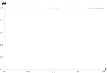
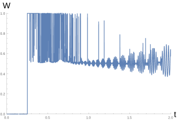
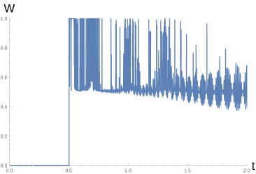
Figure 3: ( Color Online), Figures show the variation of winding number with t for different values of $\mu$. The upper panel is for the $\mu=0$, the middle panel is for $\mu=0.5$ and the lower panel is for $\mu=1$. Here $\Delta={10}^{-3}$.

III Topological phase transition from the analysis of winding number

In this section, we explicitly discuss the physics of topological to non-topological transition from the analysis of winding number calculation. We already found the analytical expressions of three Hamiltonians in momentum space. These Hamiltonians are alike to BdG Hamiltonian.

$$\ H_{(J=1,2,3)}(k)=\left[{\begin{array}[]{cc}{{\epsilon}_{k}}^{(J)}-{\mu}^{(J)}&i\Delta^{(J)}(k)\\ -i\Delta^{(J)}(k)&\mu^{(J)}-\epsilon^{(J)}_{k}\\ \end{array}}\right],\$$ (28)

where $\epsilon_{k}^{(J)}=2t^{(J)}cos(k),{\Delta}^{J}(k)=-2\Delta^{(J)}sin(k)$.
The analytical expression for $\epsilon^{(J)}_{k}$ and $\Delta^{J}(k)$ are given in the previous section.
Topological phase transition can be ascribed by the topological invariant quality. It is convenient to define this invariant quantity using the Anderson pseudo-spin approach anderson .

$${\vec{\chi(k)}}^{J=1,2,3}={\Delta(k)}^{J}\vec{y}+({\epsilon_{k}}^{J}-{\mu}^{J})\vec{z}.$$ (29)

One can write the Hamiltonian as $H^{(J=1,2,3)}(k)={\vec{\chi(k)}}^{J}.\vec{\tau}$ where $\vec{\tau}$ are Pauli matrices which act in the particle-hole basis. It is very clear from the analytical expression that the pseudo spin define in the YZ plane.

$$\hat{\chi(k)}=\frac{\vec{\chi(k)}}{|\vec{\chi(k)}|}=cos(\theta_{k})\hat{y}+sin(\theta_{k})\hat{z}$$

Here the momentum states with periodic boundary condition for a ring $T^{(1)}$ and the unit value $\hat{\chi(k)}$ exists on a unit circle $S^{(1)}$ in the YZ plane. Therefore $\theta(k)$ is a mapping. $S^{(1)}\Rightarrow T^{1}$ and the topological invariant is simply the fundamental group of the maping which is just the integer winding number. The physical interpretation of this quantity is that the unit vector $\vec{\chi}(k)$ relates in the YZ-plane around the Brillouin zone. It is only an integer number and therefore can not vary with smooth deformation of the Hamiltonian so large on the quasiparticle gap remains finite. At the point of topological phase transition the winding number changes discontinuously. A topological invariant for $\chi(k)$ is then expressed by vincent

$$W=\int\frac{dk}{4\pi}{\epsilon}_{\alpha\beta}\frac{1}{\hat{\chi}_{\alpha}}\frac{\partial{\hat{\chi}}_{\beta}}{\partial k}.$$ (31)

Here $\alpha$ and $\beta$ are $Y$ and $Z$ two components and $\epsilon_{\alpha\beta}$ is anti-symmetric tensor.
It is very clear from our study, fig.2, that at $\mu=0$ and $t=0$ system shows only the non-topological state of cavity QED lattice. Apart from $t=0$, we observe that the winding number is always one. As we go further away from the zero chemical potential, $\mu=0.5,1$, it reveals from our study that the transition occurs from the non-topological state ($W=0$) to topological ($W=1$) state. The non-topological state persists for a range of $t$ and then follows a transition to the topological state. To the best of our knowledge, this explicit study of the winding number calculation is absent in the literature of interacting light-matter system.
It is clear from this study that as we go away from $\mu=0$ the non-topological state persist for a wider range of $t$. It is related with the following relations for three different Hamiltonians.
For the Hamiltonian $H_{2}$, one can write the condition for the persistent of non-topological state is the following.

$${\delta}_{1}-2\beta=\frac{\gamma_{2}}{2}{(\frac{{\Omega}_{a}g_{b}}{\Delta_{a}}+\frac{{\Omega}_{b}g_{a}}{\Delta_{b}})}^{2}.$$ (32)

For the Hamiltonian $H_{3}$, one can write the condition for the persistent of non-topological state is the following.

$${\delta}_{1}-2\beta+8\rho-4=\frac{\gamma_{2}}{2}{(\frac{{\Omega}_{a}g_{b}}{\Delta_{a}}+\frac{{\Omega}_{b}g_{a}}{\Delta_{b}})}^{2}.$$ (33)

In fig.3, we study the behavior of winding number with t for smaller value of $\Delta={10}^{-3}$. It is clear to us from this study that the system is in the topological state for the zero chemical potential. As we away from the zero chemical potential the system is in the non-topological state, i.e. there is no sharp topological phase transition in the system. Fluctuation of the winding number is extremely large that one cannot predict about the definite topological phase transition. It can be understand in the following way, as $\Delta\rightarrow 0$, the system is simple a fermionic chain with out any spinless p-wave superconductivity in the Hamiltonian. Therefore the bulk gap of the system is absent which implies that system has no topological state with two Majorana fermion mode at the edge.

Acknowledgement: The author would like to acknowledge the several interesting and important discussions during the international school and discussion meeting on “Topological State of Matter” at Harishchandra Research Institute at Allahabad. The author would like to acknowledge the DST project, Govt. of India. Finally, author would like to acknowledge the library of Raman Research Institute for extensive help.

IV Appendix

$$\beta = \frac{1}{2}[\frac{{|{\Omega_{b}}|}^{2}}{4{\Delta}_{b}}({\Delta}_{b}-\frac{{|{\Omega_{b}}|}^{2}}{4{\Delta}_{b}}-\frac{{|{\Omega_{b}}|}^{2}}{4({\Delta}_{a}-{\Delta}_{b})}-{\gamma_{b}}{g_{b}}^{2}-{\gamma_{1}}{g_{a}}^{2}$$ (34)

$$+{\gamma_{1}}^{2}\frac{{g_{a}}^{4}}{{\Delta_{b}}}-(a\leftrightarrow b)]$$

$\gamma_{a,b}=\frac{1}{N}\sum_{k}\frac{1}{{\omega}_{a,b}-{\omega}_{k}}$ $\gamma_{1}=\frac{1}{N}\sum_{k}\frac{1}{({\omega}_{a}+{\omega}_{b})/2-{\omega}_{k}}$ and $\gamma_{2}=\frac{1}{N}\sum_{k}\frac{e^{ik}}{({\omega}_{a}+{\omega}_{b})/2-{\omega}_{k}}$ ${\delta_{1}}={\omega}_{ab}-({\omega}_{a}-{\omega}_{b})/2$, ${\Delta}_{a}={\omega}_{e}-{\omega}_{a}$. ${\Delta}_{b}={\omega}_{e}-{\omega}_{a}-({\omega}_{ab}-{\delta_{1}})$. ${{\delta}_{a}}^{k}={\omega}_{e}-{\omega}_{k}$, ${{\delta}_{b}}^{k}={\omega}_{e}-{\omega}_{k}-({\omega}_{ab}-{\delta_{1}})$, ${\omega}_{k}={\omega}_{c}+J_{c}\sum_{k}cosk$.

${\beta_{2}}=\sum_{j=a,b}\frac{{|{\Omega_{j}}|}^{2}}{4({\Delta}_{j}-\tilde{{\Delta}_{b}})}.4\tilde{\gamma_{jb}}{g_{j}}^{2}$

$$\beta_{3} = [\frac{{|{\Omega_{b}}|}^{2}}{16{{\Delta}_{b}}^{2}}(4{\Delta}_{b}-\frac{{|{\Omega_{a}}|}^{2}}{4{\Delta}_{b}}-$$ (35)

$$\frac{{|{\Omega_{b}}|}^{2}}{4({\Delta}_{a}-{\Delta}_{b})}-\frac{{|{\Omega_{b}}|}^{2}}{\Delta_{b}}-\sum_{j=a,b}\frac{{|{\Lambda_{j}}|}^{2}}{4({\Delta}_{j}-\tilde{{\Delta}_{b}})}.4{\gamma_{jb}}{g_{j}}^{2})+{\gamma_{bb}}^{2}\frac{{g_{b}}^{4}}{{\Delta_{b}}}-(a\leftrightarrow b)]$$

Here ${\gamma}_{1}=\frac{1}{N}\sum_{k}\frac{1}{\omega-{\omega}_{k}}$, ${\gamma}_{2}=\frac{1}{N}\sum_{k}\frac{e^{ik}}{\omega-{\omega}_{k}}$, ${\gamma}_{aa}={\gamma}_{bb}=\frac{1}{N}\sum_{k}\frac{1}{\omega-\omega_{k}}$.

Here $J_{z}=0$, this condition, yields the following analytical relation between the different physical parameters of the system.

$$\frac{g_{b}\Delta_{a}}{g_{a}\Delta_{b}}=\frac{\Omega_{a}}{\Omega_{b}}.$$ (36)

And also from the condition of $J_{y}=0$, i.e., $J_{1}=J_{2}$.

$$\frac{g_{a}\Delta_{a}}{g_{b}\Delta_{b}}=\frac{\Omega_{a}}{\Omega_{b}}.$$ (37)

From the above equation, We get the following relations, $g_{b}=g_{a}$ to get the transverse Ising model.
Derivation of Eq.26:
Following Ref. kote ; sig , one can write the order parameter as the sum of singlet ($\psi(k)$) and triplet ($P(k)$). The singlet and triplet component satisfy the following relation ${\psi}(k)={\psi}(-k)$ and $P(k)=-P(-k)$. One can write the general expression for order parameter as

$$\vec{\Delta}(k)=i{\psi}(k){\sigma}_{y}+iP(k){\sigma}_{y}\sigma$$ (38)

Therefore for the p-wave superconductor, one can write the mean field Hamiltonian as

$$H=\int dk[\sum_{\alpha}{\epsilon}_{\alpha}(k){c_{\alpha}(k)}^{\dagger}c_{\alpha}(k)+(i{c_{\alpha}}(k)P(k).(\sigma\sigma_{y})_{\alpha\beta}[{c_{\beta}}^{\dagger}+h.c]$$ (39)

The first part of the Hamiltonian is the single particle energy and the second part is the pairing energy. Here we consider, $P(k)=(0,-{\Delta}(k),0)$. Finally the Hamiltonian become

$$H=\int dk[\sum_{\alpha}{\epsilon}_{\alpha}(k){c_{\alpha}(k)}^{\dagger}c_{\alpha}(k)-\frac{1}{2}\sum_{\alpha}[2i\Delta(k){c_{\sigma}}^{\dagger}(k){c_{\sigma}}^{\dagger}(-k)-2i\Delta(k){c_{\sigma}}(k){c_{\sigma}}(-k)$$ (40)

In the above expression, we use ${\Delta}(k)=-{\Delta}(-k)$. Finally we can write this hamiltonian in Nambu representation

$$H=\frac{1}{2}\int dk\sum_{\alpha}{\psi_{\alpha}}^{\dagger}H_{k}{\psi}_{\alpha}(k)$$ (41)

$\psi_{\alpha}(k)=(c_{\alpha}(k),-{c_{\alpha}}^{\dagger})$. The half factor is to balance the double counting. ${H}_{k}=\left(\begin{array}[]{cc}{\epsilon}_{\alpha}(k)&-2i{\Delta}_{\alpha}(k)\\ 2i{\Delta}_{\alpha}(k)&-{\epsilon}_{\alpha}(k)\end{array}\right)$

References

• (1)
• (2) Anderi Bernivig and Taylor L. Hughes, ”Topological Insulator and Topological Superconductor”, (Princeton University Press, Princeton, 2013).
• (3) Subir Sachdev, Quantum Phase Transitions, (Cambridge University Press, 2001 ).
• (4) C. Nayak $et~{}al.$, Rev. Mod. Phys 80, 1083 (2008).
• (5) S. Horoche and J. M. Raimond 2006 in Exploring the Quantum Atoms, Cavities, and Photons, (Oxford University Press).
• (6) G. Agarwal, ”Quantum Optics”, (Cambridge University Press, Delhi 2013).
• (7) A. Y. Kitaev, Physics-Uspekhi 44, 131 (2001).
• (8) Hartmann Michael J, Fernando G S, Brando L and Plenio Martin B 2006 Nature Phys 462 849; Hartmann Michael J, Fernando G S, Brando L and Plenio Martin B 2008, Laser and Photonics Rev. 2 527.
• (9) Hartmann Michael J, Fernando G S, Brando L and Plenio Martin B 2007, Phys. Rev. Lett 99 160501.
• (10) S. Sarkar, arXiv/con-mat:1309.7742 .
• (11) E. Majorana, Nuovo Cimento 14, 171 (1937).
• (12) F. Wilczek, Majorana returns, Nature Physics 5, 614
• (13) P. Kotetes, ”Topological Insulator and Superconductors”- Notes of TKMI 2013/2014.
• (14) M. Sigrist and K. Ueda, Rev. Mod. Phys 63, 239 (1991).
• (15) C. E. Bardyn and A. Imamoglu, Phys. Rev. Lett 109, 253606 (2012).
• (16) P. W. Anderson, Phys. Rev 110, 827 (1958).
• (17) W. Vincent Liu, ”Selected Topics in Modern Many-Body Theory” in Summer School of Department of Physics at Tsinghua, University of Beijing, China (2013).