FluSI: A novel parallel simulation tool for flapping insect flight using a Fourier method with volume penalization

Abstract

FluSI, a fully parallel open source software for pseudo-spectral simulations of three-dimensional flapping flight in viscous flows, is presented. It is freely available for non-commercial use under https://github.com/pseudospectators/FLUSI. The computational framework runs on high performance computers with distributed memory architectures. The discretization of the three-dimensional incompressible Navier–Stokes equations is based on a Fourier pseudo-spectral method with adaptive time stepping. The complex time varying geometry of insects with rigid flapping wings is handled with the volume penalization method. The modules characterizing the insect geometry, the flight mechanics and the wing kinematics are described. Validation tests for different benchmarks illustrate the efficiency and precision of the approach. Finally, computations of a model insect in the turbulent regime demonstrate the versatility of the software.

1 Introduction

Flapping flight is an active interdisciplinary research field with many open questions, and numerical simulations have become an important instrument for tackling them. Here, we present the computational solution environment FluSI which is, to the best of our knowledge, the first open source code in this field.

In the literature different numerical strategies have been proposed simulating flapping flight, e.g., the use of several, overlapping grids [19], that are adapted to the geometry, or the use of moving grids with the Arbitrary Lagrangian-Eulerian method [29]. Those methods involve significant computational and implementation overhead, whose reduction has motivated the development of methods that allow for a geometry-independent discretization, such as immersed boundary methods.

In this work, we employ the volume penalization method to take the no–slip boundary condition into account. The idea of modeling solid obstacles as porous media with a small permeability has been proposed in [2]. The forcing term acts on the entire volume of the solid and not only on its surface, as it is the case in the immersed boundary methods, and corresponds to the Darcy drag. The distinctive feature of the method is the existence of rigorous convergence proofs [1, 6] showing that the solution of the penalized equations does indeed converge to the solution of the Navier-Stokes equations with no-slip boundary conditions. This approach has been extended to model not only Dirichlet conditions applied at the surface of moving, rigid and flexible obstacles [17, 9], but also to homogeneous Neumann conditions, which is relevant for studying, e.g., turbulent mixing of a passive scalar [15]. As animals forage following odor traces, this technique can potentially be attractive for insect flight simulations as well. An interesting recent development has been proposed in [13] in the context of finite-difference discretizations. Their idea is to modify the fractional step projection scheme such that the Neumann boundary condition, as introduced in [15], appears in the pressure Poisson equation. Another variant, specifically adopted to impulsively started flow, is the iterative penalization method proposed in [12]. For reviews on immersed boundary and penalization techniques we refer to [22, 27, 32].

The remainder of this article is organized as follows. First we discuss in section 2 the numerical method of FluSI’s fluid module, which is based on a spectral discretization of the three-dimensional penalized Navier–Stokes equations. Section 3 describes the module that creates the insect geometry, as well as the governing equations for free flight simulations, and we focus on the parallel implementation in section 4. Thereafter we present a validation of our software solution environment in section 5 for different test cases established in the literature, and give an outlook for applications to flapping flight in the turbulent regime in section 6. Conclusions are drawn in section 7.

2 Numerical method

2.1 Model equations

For the numerical simulation of many flapping flyers, like insects, the fluid can typically be approximated as incompressible. It is thus governed by the incompressible Navier–Stokes equations with the no–slip boundary condition on the fluid–solid interface. The numerical solution of this problem poses two major challenges. First, the pressure is a Lagrangian multiplier that ensures the divergence-free condition. Traditional numerical schemes employ a fractional step or projection method [16], requiring to solve a Poisson problem for the pressure. Second, the no-slip boundary condition must be satisfied on a possibly complicated and moving fluid–solid interface, for which boundary-fitted grids are classical approaches [35]. Since the generation of these grids may be challenging, alternatives have been developed. The principal idea is to extend the computational domain to the interior of obstacles. The boundary is then taken into account by adding supplementary terms to the Navier–Stokes equation. The technique chosen here is the volume penalization method, which is physically motivated by replacing the solid obstacle by a porous medium with small permeability $C_{\eta}$. The penalized version of the Navier–Stokes equations then reads

$$\partial_{t}\underline{u}+\underline{\omega}\times\underline{u} = -\nabla\Pi+\nu\nabla^{2}\underline{u}-\underbrace{\frac{\chi}{C_{\eta}}\left(\underline{u}-\underline{u}_{s}\right)}_{\text{penalization}}-\underbrace{\frac{1}{C_{\mathrm{sp}}}\nabla\times\frac{\left(\chi_{\mathrm{sp}}\underline{\omega}\right)}{\nabla^{2}}}_{\text{sponge}}$$ (1)

$$\nabla\cdot\underline{u} = 0$$ (2)

$$\underline{u}\left(\underline{x},t=0\right) = \underline{u}_{0}\left(\underline{x}\right)\qquad\underline{x}\in\Omega,t>0,$$ (3)

where $\underline{u}$ is the fluid velocity, $\underline{\omega}=\nabla\times\underline{u}$ is the vorticity and $\nu$ is the kinematic viscosity. The sponge term is explained in section 2.3. Eqns. (1-3) are written in dimensionless form and the fluid density $\varrho_{f}$ is normalized to unity. The nonlinear term in eqn. (1) is written in the rotational form, hence one is left with the gradient of the total pressure $\Pi=p+\frac{1}{2}\underline{u}\cdot\underline{u}$ instead of the static pressure $p$ [28]. This formulation is chosen because of its favorable properties when discretized with spectral methods, namely conservation of momentum and energy [28, pp. 210]. At the exterior of the computational domain, which is supposed to be sufficiently large, periodic boundary conditions can be assumed. The mask function $\chi$ is defined as

$$\chi\left(\underline{x},t\right)=\left\{\begin{array}[]{cc}0&\text{if }\underline{x}\in\Omega_{f}\\ 1&\text{if }\underline{x}\in\Omega_{s}\end{array}\right.,$$ (4)

where $\Omega_{f}$ is the fluid and $\Omega_{s}$ the solid domain. In anticipation of the application to moving boundaries, we note that we will replace the discontinuous $\chi$-function by a smoothed one, with a thin smoothing layer centered around the interface. The mask function encodes all geometric information of the problem, and eqns. (1-3) do not include no–slip boundary conditions.

Note that in the fluid domain $\Omega_{f}$ one recovers the original equation as the penalization term $\frac{\chi}{C_{\eta}}\left(\underline{u}-\underline{u}_{s}\right)$ vanishes. The convergence proof in [6, 1] shows that the solution of the penalized Navier–Stokes equations (1-3) tends for $C_{\eta}\rightarrow 0$ indeed towards the exact solution of Navier–Stokes imposing no-slip boundary conditions, with a convergence rate of $\mathcal{O}\left(\sqrt{C_{\eta}}\right)$ in the $L^{2}$–norm. The parameter $C_{\eta}$ should thus be chosen to a small enough value, which is also intuitively clear by the physical interpretation of $C_{\eta}$ as permeability. However, the choice of $C_{\eta}$ is subject to constraints, as the penalized equations are discretized and solved numerically. The modeling error of order $\mathcal{O}\left(\sqrt{C_{\eta}}\right)$ should be of the same order as the discretization error [24]. It is first noted that in eqn. (1), $C_{\eta}$ has the dimension of a time. It is instructive to put the nonlinear, viscous and pressure terms aside for a moment. One is then left with $\partial_{t}u=-u/C_{\eta}$ inside the solid, with the obvious solution $u=u_{0}\exp\left(-t/C_{\eta}\right)$. Thus, $C_{\eta}$ can be directly identified as the relaxation time. Interfering with the time step $\Delta t$, usually implying $\Delta t=\mathcal{O}\left(C_{\eta}\right)$, this simple fact has important consequences for the numerical solution. It indicates that a good choice for $C{}_{\eta}$ is not only “small enough”, but also “as large as possible”. Further insight in the properties of the penalization method can be obtained considering the penalization boundary layer of width $\delta_{\eta}=\sqrt{\nu C_{\eta}}$, which forms inside the obstacle $\Omega_{s}$, as shown in [6]. When increasing the resolution, the number of points per boundary layer thickness, $K=\delta_{\eta}/\Delta x$, should be kept constant, which implies the relation $C_{\eta}\propto\left(\Delta x\right)^{2}$, consistent with [24], where the penalized Laplace and Stokes operators were analyzed analytically and numerically. With the scaling for $C_{\eta}$, one still has to choose the constant $K$. In fact, for any value of $K$, the method will converge with the same convergence rate, but the error offset can be tuned. For the two-dimensional Couette flow, in [9] we reported the optimal value of $K=0.128$. In a range of numerical validation tests, including the ones presented here, we find $K=0.1-0.4$ as a good choice which we recommend as a guideline for practical applications.

To satisfy the incompressibility constraint (2), a Poisson equation for the pressure is derived by taking the divergence of eqn. (1), yielding

$$\nabla^{2}\Pi = \nabla\cdot\left(-\underline{\omega}\times\underline{u}-\frac{\chi}{C_{\eta}}\left(\underline{u}-\underline{u}_{s}\right)\right).$$ (5)

By construction of the method, eqn. (5) can be solved with periodic boundary conditions.

The aerodynamic force $\underline{F}$ and the torque moment $\underline{m}$, both important quantities in the present applications, can be computed from

$$\underline{F} = \oint_{\partial\Omega_{s}}\sigma\cdot\underline{n}\,\mathrm{d}\gamma=\frac{1}{C_{\eta}}\int_{\Omega}\chi\left(\underline{u}-\underline{u}_{s}\right)\mathrm{d}V+\frac{\mathrm{d}}{\mathrm{d}t}\int_{\Omega_{s}}\underline{u}_{s}\mathrm{d}V$$ (6)

$$\underline{m} = \oint_{\partial\Omega_{s}}\underline{r}\times\left(\sigma\cdot\underline{n}\right)\,\mathrm{d}\gamma=\frac{1}{C_{\eta}}\int_{\Omega}\underline{r}\times\chi\left(\underline{u}-\underline{u}_{s}\right)\mathrm{d}V+\frac{\mathrm{d}}{\mathrm{d}t}\int_{\Omega_{s}}\underline{r}\times\underline{u}_{s}\mathrm{d}V,$$ (7)

where the additional terms are denoted ‘unsteady corrections’ [36].

2.2 Penalization method for moving boundary problems

The volume penalization method as discussed so far assumes a discontinuous mask function in the form of eqn. (4). When applying the method to a non-grid aligned body, for example a circular cylinder, the mask function geometrically approximates the boundary to first order in $\Delta x$. Results for stationary cylinder using the discontinuous mask function are acceptable [31, 33], but spurious oscillations in the case of moving ones are reported [17]. The reason is that the discontinuous mask can be translated only by integer multiples of the grid spacing, and this jerky motion causes large oscillations in the aerodynamic forces. Kolomenskiy and Schneider [17] proposed an algorithm to shift the mask function in Fourier space instead of physical space. In the present work, we employ a different approach, because displacing the mask in Fourier space involves (additional) Fourier transforms, which are computationally expensive, especially if more than one rigid body is considered, as it is the case here. The idea on hand is to directly assume the mask function to be smoothed over a thin smoothing layer [8, 9]. To this end, we introduce the signed distance function $\delta(\underline{x},t)$ [25], and the mask function can then be computed from the signed distance, using

$$\chi\left(\delta\right)=\left\{\begin{array}[]{cc}1&\delta\leq-h\\ \frac{1}{2}\left(1+\cos\left(\pi\frac{\delta+h}{2h}\right)\right)&-h<\delta<+h\\ 0&\delta>+h\end{array}\right.$$ (8)

where the semi-thickness of the smoothing layer, $h$, is used. It is typically defined relative to the grid size, $h=C_{\mathrm{smth}}\Delta x$, thus eqn. (8) converges to a Heaviside step function as $\Delta x\rightarrow 0$. Nonetheless, it can be translated by less than one grid point, and then be resampled on the Eulerian fluid grid.

2.3 Wake removal techniques

The penalized Navier–Stokes equations (1-3) do, by principle, not include no-slip boundary conditions and furthermore we discretize them in a periodic domain $\Omega$. In such a periodic setting, the wake re-enters the domain, which is an undesired artifact. To overcome it, a supplementary “sponge” penalization term can be added to the vorticity-velocity formulation of the Navier-Stokes equations, in order to gradually damp the vorticity [8, 9]. The sponge penalization parameter $C_{\mathrm{sp}}$ is usually set to a larger value than $C_{\eta}$, typically $C_{\mathrm{sp}}=10^{-1}$. The larger value and its longer relaxation time ensure that if a traveling vortex pair enters the sponge region, the leading one is not dissipated too fast, because it otherwise could leave the partner orphaned in the domain. Applying the Biot-Savart operator to the vorticity-velocity formulation we formally find $-\frac{1}{C_{\mathrm{sp}}}\nabla\times\frac{\left(\chi_{\mathrm{sp}}\underline{\omega}\right)}{\nabla^{2}}$. By construction the sponge term is divergence-free, which is important since otherwise it would contribute to the pressure, which in turn would be modified even in regions far away from the sponge due to its nonlocality. Moreover, it leaves the mean flow, i.e., the zeroth Fourier mode, unchanged. This technique is well adapted to spectral discretizations, since computing the sponge term requires the solution of three Poisson problems, which becomes a simple division in Fourier space. A discussion on the influence of the vorticity sponge can be found in section 6 and Fig. 13.

Dirichlet conditions on the velocity can be imposed directly with the volume penalization, which applies for example to channel walls. For simulations in a uniform, unbounded free-stream, we use both techniques; in a small layer at the domain borders, the Dirichlet condition $\underline{u}=\underline{u}_{\infty}$ is imposed with the same precision as the actual obstacle, and a preceding, thicker sponge layer ensures that the upstream influence is minimized [9]. The sponge technique is similar to the “fringe regions” proposed in [30]. However, in [30] only a velocity sponge has been used, which corresponds to the penalization term, i.e., $-\chi_{\mathrm{sp}}\left(\underline{u}-\underline{u}_{\mathrm{sp}}\right)/C_{\mathrm{sp}}$. The vorticity sponge idea has the advantage of not requiring a “desired” velocity field $\underline{u}_{\mathrm{sp}}$, which has to be set a priori. It also does not contribute to the pressure, which helps reducing the region of influence.

2.4 Discretization

The model equations (1) and (5) can be discretized with any numerical scheme, in particular a Fourier pseudo-spectral discretization can be used [31, 17, 9]. The general idea is to represent field variables as truncated Fourier series, thus in three dimensions we have for any quantity $\varphi$ (velocity, pressure, vorticity) the discrete complex Fourier coefficients $\widehat{\varphi}$. They can be computed efficiently with the fast Fourier transform (FFT) [7]. The gradient of a scalar $q$ can be obtained by multiplying the Fourier coefficients $\widehat{q}$ with the wavevector $\underline{k}=\left(k_{x},k_{y},k_{z}\right)^{T}$ and the complex unit, $\widehat{\nabla q}=\iota\underline{k}\widehat{q}$. The Laplace operator becomes a simple multiplication by $-\left|\underline{k}\right|^{2}$. When using, e.g., finite differences, the dominant part of computational efforts is spent on solving the Poisson equation in every time step [14]. This is a strong motivation to employ a Fourier discretization, as inverting a diagonal operator becomes a simple division. Inserting the truncated Fourier series into the model equations and requiring that the residual vanishes with respect to all test functions (which are identical with the trial functions $\exp\left(\iota\underline{k}\cdot\underline{x}\right)$ ) yields a Galerkin projection and results in an evolution equation for the Fourier coefficients of the velocity. The nonlinear and penalization terms contain products, which become convolutions in Fourier space. To speed-up computation, the products are calculated in physical space. This last introduces aliasing errors which are virtually eliminated by the 2/3 rule [5], meaning that only 2/3 of the Fourier coefficients are retained. Such a mixture of spectral and physical computations is generally labeled "pseudo-spectral" and is, when de-aliased, equivalent to a Fourier-Galerkin scheme. The code can be run with and without dealiasing, but our choice is to conservatively always turn dealiasing on. More details on the effect of dealiasing are discussed in [24, p. 318].

The spatially discretized equations can then be advanced in time in Fourier space. The code provides a classical fourth order Runge–Kutta with explicit treatment of the diffusion term, and a second order Adams–Bashforth scheme with integrating factor [31].

Besides the fast solution of Poisson problems, the spectral method has the advantage of not adding numerical diffusion or dispersion to the penalized equation, unlike it is the case when discretized with finite differences. Furthermore, most of the computational effort is concentrated in the Fourier transforms, which is advantageous from a computational point of view. However, the discretization requires the use of an equidistant grid, which implies a large number of grid points to resolve the thin boundary layers.

Note that we do not explicitly apply a Neumann-type boundary condition for the pressure in our method. We only use periodic boundary conditions in the computational domain, which are natural for Fourier methods. It was shown in [1] that the pressure field of the penalized problem converges to the pressure in the original boundary value problem. The discretization that we use is consistent and stable, therefore the numerical solution converges to the exact solution of the continuous penalized problem.

3 Virtual insect model

We previously described the fluid module where the geometry is taken into account by the penalization method, which is the interface with the insect module described next.

Insects fly by flapping their wings, which are basically flat with sharp edges and operate typically at high angle of attack. In the following, we describe the insect framework used in this work in detail, the essential task being to construct $\chi$ and $\underline{u}_{s}$ which enter eqn. (1). The virtual insect consists of a body and two wings, all of which are performing solid body rotations around three axes and assumed to be rigid. Therefore, we will make use of the rotation matrices

$$R_{x}\left(\xi\right)=\left(\begin{array}[]{ccc}1&0&0\\ 0&\cos\xi&\sin\xi\\ 0&-\sin\xi&\cos\xi\end{array}\right) R_{y}\left(\xi\right)=\left(\begin{array}[]{ccc}\cos\xi&0&-\sin\xi\\ 0&1&0\\ \sin\xi&0&\cos\xi\end{array}\right)$$

$$R_{z}\left(\xi\right)=\left(\begin{array}[]{ccc}\cos\xi&\sin\xi&0\\ -\sin\xi&\cos\xi&0\\ 0&0&1\end{array}\right)$$

and define the different reference frames, namely the global $\underline{x}^{(g)}$, body $\underline{x}^{(b)}$, stroke plane $\underline{x}^{(s)}$ and wing $\underline{x}^{(w)}$, in which the geometry is defined. As described above, the mask function is constructed in each evaluation of the right hand side as a function of the signed distance function, $\chi\left(\underline{x}\right)=\chi\left(\delta\left(\underline{x}\right)\right)$, according to eqn. (8).

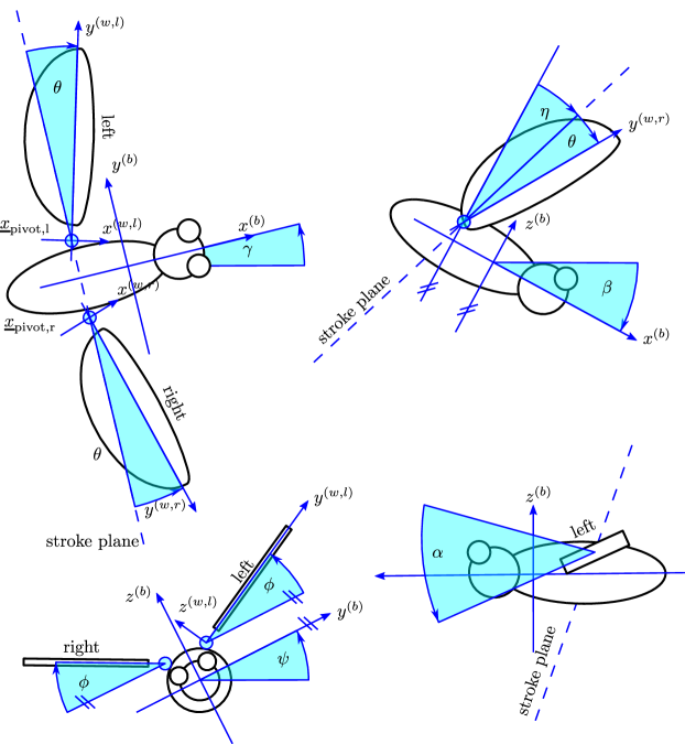
Figure 1: Model insect with definitions of the body angles $\gamma$ (yaw), $\beta$ (pitch), $\psi$ (roll), the anatomical stroke plane angle $\eta$, the wing coordinate systems and the wing angles $\theta$ (deviation), $\phi$ (position) and $\alpha$ (feathering). All angles are shown with positive sign.

3.1 Body system

The insect’s body is responsible for a major part of the total drag force. It is described by its logical center $\underline{x}_{\mathrm{cntr}}^{(g)}$, the translational velocity $\underline{u}_{\mathrm{cntr}}^{(g)}$ and the body angles $\beta$ (pitch), $\gamma$ (yaw) and $\psi$ (roll), see figure 1 The center point $\underline{x}_{\mathrm{cntr}}^{(g)}$ does not necessarily coincide with the center of gravity, it is rather an arbitrary point of reference. A point $\underline{x}^{(g)}$ in the global coordinate system can be transformed to the body system using the following linear transformation

$$\underline{x}^{(b)} = M_{\mathrm{body}}\left(\psi,\beta,\gamma\right)\left(\underline{x}^{(g)}-\underline{x}_{\mathrm{cntr}}^{(g)}\right)$$

$$M_{\mathrm{body}} = R_{x}\left(\psi\right)R_{y}\left(\beta\right)R_{z}\left(\gamma\right).$$ (11)

Since rotation matrices do not commute, it is important to note that the body is first yawed, then pitched and finally rolled, which is conventional in flight mechanics. The geometry of the body is defined in the body reference frame. The angular velocity of the body in the global system is

$$\underline{\Omega}_{b}^{(g)} = R_{z}^{-1}\left(\gamma\right)\left[\left(\begin{array}[]{c}0\\ 0\\ \dot{\gamma}\end{array}\right)+R_{y}^{-1}\left(\beta\right)\left[\left(\begin{array}[]{c}0\\ \dot{\beta}\\ 0\end{array}\right)+R_{x}^{-1}\left(\psi\right)\left(\begin{array}[]{c}\dot{\psi}\\ 0\\ 0\end{array}\right)\right]\right]$$

$$\underline{\Omega}_{b}^{(b)} = M_{\mathrm{body}}\>\Omega_{b}^{(g)}$$

which defines the velocity field inside the insect resulting from the body motion,

$$\underline{u}_{b}^{(g)}=\underline{u}_{\mathrm{cntr}}^{(g)}+M_{\mathrm{body}}^{-1}\left(\underline{\Omega}_{b}^{(b)}\times\underline{x}^{(b)}\right).$$ (13)

Equation (13) is valid also in the wings, since the flapping motion is prescribed relative to the body.

3.2 Body shape

The body shape is described in the body reference frame described previously. For instance, for the body depicted in figure 1, which is composed of an ellipsoidal shaped thorax and spheres for the head and eyes, the signed distance function is the intersection of the distance functions for the thorax, head and eyes,

$$\delta_{\mathrm{body}}=\max\left(\delta_{\mathrm{thorax}},\delta_{\mathrm{head}},\delta_{\mathrm{eyes}}\right).$$ (14)

The $\max$ operator of the signed distances in eqn. (14) represents the intersection operator [25]. The signed distances for the components read

$$\delta_{\mathrm{thorax}}\left(\underline{x}^{(b)}\right) = \sqrt{\left(y^{(b)}\right)^{2}+\left(z^{(b)}\right)^{2}}-\sqrt{b^{2}\left(1-\left(x^{(b)}/a\right)^{2}\right)}$$

$$\delta_{\mathrm{head}}\left(\underline{x}^{(b)}\right) = \left|\underline{x}^{(b)}-\underline{x}_{0,\mathrm{head}}^{(b)}\right|$$

$$\delta_{\mathrm{eyes}}\left(\underline{x}^{(b)}\right) = \left|\underline{x}^{(b)}-\underline{x}_{0,\mathrm{eyes}}^{(b)}\right|,$$

where $a$, $b$ define the axes of the thorax ellipsoid and $\underline{x}_{0,\mathrm{head,eyes}}^{(b)}$ are the centers of the spheres.

3.3 Wing system

We consider only insects with two wings, one on each side, that are rotating about the pivot points $\underline{x}_{\mathrm{pivot,r}}^{(b)}$ and $\underline{x}_{\mathrm{pivot,l}}^{(b)}$. These pivots do not necessarily lie on the body surface; we rather allow a gap between wings and body. This gap avoids problems with non-solenoidal velocity fields at the wing base. It is conventional to introduce a stroke plane, which is a plane tilted with respect to the body by an angle $\eta$. The coordinate in the stroke plane reads

$$\underline{x}^{(s)}=M_{\mathrm{stroke}}\left(\underline{x}^{(b)}-\underline{x}_{\mathrm{pivot}}^{(b)}\right).$$

Here, we use an anatomical stroke angle, that is, the angle $\eta$ is defined relative to the body. Within the stroke plane, the wing motion is described by the angles $\alpha$ (feathering angle or angle of attack), $\phi$ (positional or flapping angle), $\theta$ (deviation or out-of-stroke angle). Applying two rotation matrices yields the transformation from the body to the wing coordinate system:

$$\underline{x}^{(w)}=M_{\mathrm{wing}}\underline{x}^{(s)}=M_{\mathrm{wing}}M_{\mathrm{stroke}}\left(\underline{x}^{(b)}-\underline{x}_{\mathrm{pivot}}^{(b)}\right).$$

When flapping symmetrically, i.e., both wings following the same motion protocol, the stroke and wing rotation matrices for the left and right wing are given by

$$M_{\mathrm{stroke,l}}=R_{y}\left(\eta\right) M_{\mathrm{stroke,r}}=R_{x}\left(\pi\right)R_{y}\left(\eta\right)$$

$$M_{\mathrm{wing,l}}=R_{y}\left(\alpha\right)R_{z}\left(-\theta\right)R_{x}\left(\phi\right) M_{\mathrm{wing,r}}=R_{y}\left(-\alpha\right)R_{z}\left(-\theta\right)R_{x}\left(-\phi\right)$$

due to the rotation $R_{x}\left(\pi\right)$ the sign of $\theta$ for the right wing does not have to be inverted. The angular velocities of the wings are given by

$$\underline{\Omega}_{w}^{(b)} = M_{\mathrm{stroke}}^{-1}\left[R_{x}^{-1}\left(\phi\right)\left[\left(\begin{array}[]{c}\dot{\phi}\\ 0\\ 0\end{array}\right)+R_{z}^{-1}\left(-\theta\right)\left[\left(\begin{array}[]{c}0\\ 0\\ -\dot{\theta}\end{array}\right)+R_{y}^{-1}\left(\alpha\right)\left(\begin{array}[]{c}0\\ \dot{\alpha}\\ 0\end{array}\right)\right]\right]\right]$$

$$\underline{\Omega}_{w}^{(w)} = M_{\mathrm{wing}}\>\underline{\Omega}_{w}^{(b)}$$

which is used to compute the velocity field resulting from the wing motion,

$$\underline{u}_{w}^{(w)} = \underline{\Omega}_{w}^{(w)}\times\underline{x}^{(w)}$$

$$\underline{u}_{w}^{(g)} = M_{\mathrm{body}}^{-1}\;M_{\mathrm{wing}}^{-1}\;M_{\mathrm{stroke}}^{-1}\;\underline{u}_{w}^{(w)}.$$ (16)

The total velocity field inside the wings is given as the superposition of the body and wing rotation,

$$\underline{u}_{s}^{(g)}\left(\underline{x}\in\left\{\underline{x}_{w}\right\}\right)=\underline{u}_{w}^{(g)}+\underline{u}_{b}^{(g)}.$$

The actual kinematics, i.e., the angles $\alpha\left(t\right)$, $\phi\left(t\right)$ and $\theta\left(t\right)$ are parametrized by either Fourier or Hermite interpolation coefficients and read from a *.ini file.

3.4 Wing shape

In the previous section we defined the wing reference frame $\underline{x}^{(w)}$, in which we now describe the wing’s signed distance function $\delta$. In general, we define a set of several signed distance functions, each of which describes one surface of the wing. The signed distance function of the entire wing is then given by their intersection. For some model insects, we consider simple wings for which straightforward analytical expressions are available. For a rectangular wing, for instance the one illustrated in figure 6 (c), we find for the signed distance function

$$\delta\left(\underline{x}^{(w)}\right)=\max\left(x^{(w)}-b;x^{(w)}-\left(B-b\right);y^{(w)}-1;a-y^{(w)};\left|z\right|-h/2\right).$$ (17)

For realistic insect wings however, we parametrize the wing shape in polar coordinates. As illustrated in figure 2, the shape in the wing plane is described by the center point $\underline{x}_{c}^{(w)}$, which is arbitrary as long as the function $R\left(\vartheta\right)$ is unique for all $\vartheta$. To sample the wing on a computational grid, we need a function $R\left(\vartheta\right)$ that can be evaluated for all $\vartheta$. As $R\left(\vartheta\right)$ is naturally $2\pi$-periodic, a truncated Fourier series can be used:

$$R\left(\vartheta\right)=\frac{a_{0}}{2}+\sum_{i=1}^{N}a_{i}\cos\left(2\pi i\vartheta\right)+\sum_{i=1}^{N}b_{i}\sin\left(2\pi i\vartheta\right)$$ (18)

In practice, eqn (18) has to be evaluated for all grid points in the vicinity of the wing, which requires $\mathcal{O}\left(N_{x}N_{y}N_{z}\right)$ evaluations with a small constant. The computational cost can however be significant, which is why eqn. (18) is evaluated for 25 000 values of $\vartheta$ once during initialization. Afterwards, linear interpolation is used for its lower computational cost. The signed distance for such a wing then reads

$$\delta\left(\underline{x}^{(w)}\right)=\max\left(\left|z^{(w)}\right|-h/2;r\left(\vartheta\right)-R\left(\vartheta\right)\right).$$

If a wing cannot be described by one radius, because $R\left(\vartheta\right)$ is not unique, several radii and center points can be used [4].

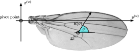
Figure 2: Realistic wing shapes are described in polar coordinates $R\left(\vartheta\right)$.

3.5 Power requirement

Actuating the wings requires power expenditures that are very difficult to measure directly. In numerical simulations, the power can be obtained directly, since the aerodynamic torque moment $\underline{m}$ with respect to the wing pivot point is available from eqn. (7). The power $P_{\mathrm{aero}}$ required to move one wing is found to be

$$P_{\mathrm{aero}}=-\underline{m}\cdot\left(\underline{\Omega}_{w}-\underline{\Omega}_{b}\right)$$ (19)

which is equivalent to the definition $P_{\mathrm{aero}}=\int\underline{u}\mathrm{d}\underline{F}$ given in [21]. In addition to the aerodynamic power, the inertial power has to be expended, i.e., the power required to move the wing in vacuum. As the flapping motion is periodic, its stroke averaged value is zero. The inertial power $P_{\mathrm{inert}}$ is positive if the wing is accelerated (power consumed) and negative if it is decelerated. The definition is

$$P_{\mathrm{inert}}=\underline{\Omega}_{w}^{(w)}\cdot\left(\underline{\underline{J}}^{(w)}\underline{\dot{\Omega}}_{w}^{(w)}+\underline{\Omega}_{w}^{(w)}\times\underline{\underline{J}}^{(w)}\underline{\Omega}_{w}^{(w)}\right)$$

with the wing tensor of inertia $\underline{\underline{J}}^{(w)}$ [3]. The sum of inertial and aerodynamic power can be negative during deceleration phases, which would mean that the insect can store energy in its muscles. It is unknown to what extent this can be realized, and it is thus often conservatively assumed that energy storage is not possible, in which case the total power $P_{\mathrm{total}}$ is given by $P_{\mathrm{total}}=\max\left(P_{\mathrm{inert}}+P_{\mathrm{aero}},0\right).$

3.6 Governing equations in free flight

Until now we have considered the insect to be fixed, i.e., tethered in the computational domain. In free flight, additional equations have to be solved together with the fluid, namely Newton’s law. The body translation is then governed by

$$M\,\underline{\dot{u}}_{\mathrm{cntr}}^{(g)}=\underline{F}^{(g)}$$

where $\underline{F}^{(g)}$ contains the aerodynamic and gravitational forces and $M$ is the mass of the insect. For simplicity, $\underline{x}_{\mathrm{centr}}$ and $\underline{u}_{\mathrm{centr}}$ correspond to the center of gravity in the case of free flight. To handle the rotational degrees of freedom, we employ a quaternion based formulation, similar to the one proposed in [20], which avoids the ‘Gimbal lock’ problem. The governing equation for the angular velocity $\underline{\Omega}^{(b)}$ in the body reference frame reads

$$\underline{\underline{J}}^{(b)}\dot{\underline{\Omega}}^{(b)}+\left(\begin{array}[]{ccc}0&-\Omega_{z}^{(b)}&\Omega_{y}^{(b)}\\ \Omega_{z}^{(b)}&0&-\Omega_{x}^{(b)}\\ -\Omega_{y}^{(b)}&\Omega_{x}^{(b)}&0\end{array}\right)\underline{\underline{J}}^{(b)}\underline{\Omega}^{(b)}=\underline{m}^{(b)},$$

where $\underline{\underline{J}}^{(b)}$ is the moment of inertia around the body axes $\left(x^{(b)},y^{(b)},z^{(b)}\right)$ and $\underline{m}$ is the vector of torque moments as defined in eqn. (7). The skew-symmetric term stems from the change into a moving reference frame. We introduce the normalized quaternion $\varepsilon$ with components $\varepsilon_{i}$, $i=0,\ldots,3$, $\sum\varepsilon_{i}^{2}=1$. The governing equations for the quaternion state are

$$\dot{\underline{\varepsilon}}=\frac{1}{2}\underline{\underline{S}}^{T}\,\underline{\Omega}^{(b)}$$

with the matrix

$$S=\left(\begin{array}[]{cccc}-\varepsilon_{1}&\varepsilon_{0}&\varepsilon_{3}&-\varepsilon_{2}\\ -\varepsilon_{2}&-\varepsilon_{3}&\varepsilon_{0}&\varepsilon_{1}\\ -\varepsilon_{3}&\varepsilon_{2}&-\varepsilon_{1}&\varepsilon_{0}\end{array}\right).$$

Assuming $\underline{\underline{J}}^{(b)}$ to be constant the body axes to be the prinicipal axes of inertia (i.e., $\underline{\underline{J}}^{(b)}$ is diagonal), the following first order system set of 13 equations is obtained

$$\frac{\mathrm{d}}{\mathrm{d}t}\left(\begin{array}[]{c}x_{\mathrm{cntr}}^{(g)}\\ y_{\mathrm{cntr}}^{(g)}\\ z_{\mathrm{cntr}}^{(g)}\\ u_{\mathrm{cntr,x}}^{(g)}\\ u_{\mathrm{cntr,y}}^{(g)}\\ u_{\mathrm{cntr,z}}^{(g)}\\ \varepsilon_{0}\\ \varepsilon_{1}\\ \varepsilon_{2}\\ \varepsilon_{3}\\ \Omega_{x}^{(b)}\\ \Omega_{y}^{(b)}\\ \Omega_{z}^{(b)}\end{array}\right) = \left(\begin{array}[]{c}u_{\mathrm{cntr,x}}^{(g)}\\ u_{\mathrm{cntr,y}}^{(g)}\\ u_{\mathrm{cntr,z}}^{(g)}\\ F_{x}^{(g)}/M\\ F_{y}^{(g)}/M\\ \left(F_{z}^{(g)}/M-g\right)\\ \left(-\varepsilon_{1}\Omega_{x}^{(b)}-\varepsilon_{2}\Omega_{y}^{(b)}-\varepsilon_{3}\Omega_{z}^{(b)}\right)/2\\ \left(\varepsilon_{0}\Omega_{x}^{(b)}-\varepsilon_{3}\Omega_{y}^{(b)}+\varepsilon_{2}\Omega_{z}^{(b)}\right)/2\\ \left(\varepsilon_{3}\Omega_{x}^{(b)}+\varepsilon_{0}\Omega_{y}^{(b)}-\varepsilon_{1}\Omega_{z}^{(b)}\right)/2\\ \left(-\varepsilon_{2}\Omega_{x}^{(b)}+\varepsilon_{1}\Omega_{y}^{(b)}+\varepsilon_{0}\Omega_{z}^{(b)}\right)/2\\ \left(\left(J_{y}^{(b)}-J_{z}^{(b)}\right)\Omega_{y}^{(b)}\Omega_{z}^{(b)}+m_{x}^{(b)}\right)/J_{x}^{(b)}\\ \left(\left(J_{z}^{(b)}-J_{x}^{(b)}\right)\Omega_{z}^{(b)}\Omega_{x}^{(b)}+m_{y}^{(b)}\right)/J_{y}^{(b)}\\ \left(\left(J_{x}^{(b)}-J_{y}^{(b)}\right)\Omega_{x}^{(b)}\Omega_{y}^{(b)}+m_{z}^{(b)}\right)/J_{z}^{(b)}\end{array}\right)$$ (46)

which is solved with the same time discretization as the fluid. The rotation matrix $M_{body}$ is then computed from the quaternion $\varepsilon_{i}$

$$M_{body}=\left(\begin{array}[]{ccc}\varepsilon_{0}^{2}+\varepsilon_{1}^{2}-\varepsilon_{2}^{2}-\varepsilon_{3}^{2}&2\left(\varepsilon_{1}\varepsilon_{2}-\varepsilon_{3}\varepsilon_{0}\right)&2\left(\varepsilon_{1}\varepsilon_{3}+\varepsilon_{2}\varepsilon_{0}\right)\\ 2\left(\varepsilon_{1}\varepsilon_{2}+\varepsilon_{3}\varepsilon_{0}\right)&\varepsilon_{0}^{2}-\varepsilon_{1}^{2}+\varepsilon_{2}^{2}-\varepsilon_{3}^{2}&2\left(\varepsilon_{2}\varepsilon_{3}-\varepsilon_{1}\varepsilon_{0}\right)\\ 2\left(\varepsilon_{1}\varepsilon_{3}-\varepsilon_{2}\varepsilon_{0}\right)&2\left(\varepsilon_{2}\varepsilon_{3}+\varepsilon_{1}\varepsilon_{0}\right)&\varepsilon_{0}^{2}-\varepsilon_{1}^{2}-\varepsilon_{2}^{2}+\varepsilon_{3}^{2}\end{array}\right),$$ (47)

which replaces the definition in eqn. (11) in the free-flight case. The initial values at time $t=0$ for $\varepsilon_{i}$ can conveniently be computed from a set of yaw, pitch and roll angles,

$$\left(\begin{array}[]{c}\varepsilon_{0}\\ \varepsilon_{1}\\ \varepsilon_{2}\\ \varepsilon_{3}\end{array}\right)=\left(\begin{array}[]{c}\cos\left(\psi/2\right)\cos\left(\beta/2\right)\cos\left(\gamma/2\right)+\sin\left(\psi/2\right)\sin\left(\beta/2\right)\sin\left(\gamma/2\right)\\ \sin\left(\psi/2\right)\cos\left(\beta/2\right)\cos\left(\gamma/2\right)-\cos\left(\psi/2\right)\sin\left(\beta/2\right)\sin\left(\gamma/2\right)\\ \cos\left(\psi/2\right)\sin\left(\beta/2\right)\cos\left(\gamma/2\right)+\sin\left(\psi/2\right)\cos\left(\beta/2\right)\sin\left(\gamma/2\right)\\ \cos\left(\psi/2\right)\cos\left(\beta/2\right)\sin\left(\gamma/2\right)-\sin\left(\psi/2\right)\sin\left(\beta/2\right)\cos\left(\gamma/2\right)\end{array}\right).$$

In the actual implementation, we multiply the right hand side of equation (46) with a six component vector with zeros or ones, to deactivate some degrees of freedom.

4 Parallel implementation

Until now we described the numerical method employed by the FluSI code, which is based on the volume penalization method combined with a pseudo-spectral discretization. This framework allows for a high degree of modularization, since all geometry is encoded in the mask function and the solid velocity field. The framework is intended to be applicable also for higher Reynolds number flow, for which small spatial and temporal vortical structures appear. To resolve these scales, high resolution and therefore the usage of high-performance computers is required. To this end, our code is designed to compute on massively parallel machines with distributed memory architectures. The parallel implementation is based on the MPI protocol and written in FORTRAN95.

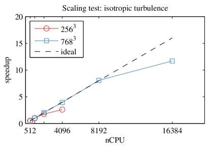
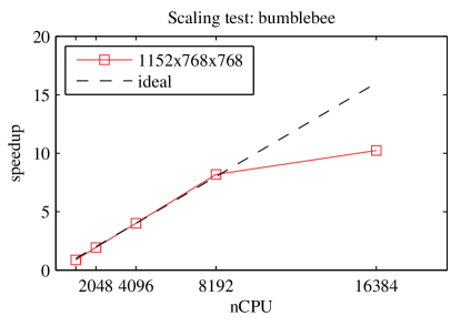
Figure 3: Parallel scaling tests on a large-scale computing cluster of type IBM BlueGene/Q. Left: isotropic turbulence simulation without insect, for two different resolutions. Fifty time steps have been performed. The reference simulation is the 1024 run. Right: scaling test for a bumblebee simulation (see section 6). Two complete strokes have been computed, and the timing is averaged over the second one. The reference simulation is the 2048 cores run.

For the fluid part the P3DFFT library is used to compute the 3D Fourier transforms [26]. This library provides a parallel data decomposition framework, and employs the FFTW library [11] for the one–dimensional Fourier transforms. The flow variables are stored on the three–dimensional Cartesian computational grid. Each MPI process only holds a portion of the total data, and the parallel decomposition is performed on at most two indices, i.e., a pencil decomposition is used. The $x$-direction is not split among processes, the code can thus run on $N_{y}N_{z}$ processes at most. This limitation is however not of practical importance, since $N_{y}N_{z}$ usually exceeds the number of available CPUs by orders of magnitude. Besides the Fourier transforms, the operations are local, i.e., they do not require inter-processor communication. The parallel scaling test for the fluid module is shown in Fig. 3 (left), for the case of an isotropic turbulence simulation and two different problem sizes, $256^{3}$ and $768^{3}$. The latter shows good scaling up to 8192 CPU on the IBM BlueGene/Q machine used for the tests.

The insect module is used to generate the $\chi$-function and the solid body velocity field $\underline{u}_{s}$. It is crucial that the implementation does not spoil the favorable scaling properties. The module is therefore designed around an derived insect datatype called diptera, which holds all properties of the insect, such as the wing shape, body position and Fourier coefficients of the wing kinematics. This object is of negligible size, and therefore each MPI process holds a copy of it. The task to construct the penalization term is then again completely local. Forces and torques (eqn. (6-7)) are computed efficiently with the MPI_allreduce command. It is further necessary to distinguish between distinct parts of the mask function, e.g., body and wings and possibly outer boundary conditions, like channel walls. To accomplish this, we introduce the concept of mask coloring, i.e., we allocate a second integer*2 array for the mask function that holds the value of the mask color. This allows to easily exclude for example channel walls from the force computation in eqn. (6), and limits the memory footprint to two arrays. We further use it to compute the forces acting on the body and wings individually. If the insect’s body is tethered, there is no need to reconstruct it every time the mask is updated. The mask coloring can in this case be used easily to delete only the wings from the mask function while keeping the body in memory. This reduces the CPU time requirement of the mask function, since the body occupies a relatively large volume (compared to the wings) and consequently a larger number of grid points are affected.

Fig. 3 (right) shows the scaling test of an insect simulation. The insect model is the bumblebee presented in section 6, but the scaling behavior is the same for any other model. We computed two complete strokes at a resolution of $1152\times 768\times 768$, and the elapsed walltime was measured for the second one. The parallel scaling is virtually the same as in the pure fluid case, indicating that the insect module does indeed not spoil parallel scaling efficiency.

1. Initialization. Read parameters from *.ini file, allocate memory, set up fluid initial condition, initialize P3DFFT

2. Begin loop over time step

   1. Generate mask function $\chi\left(\underline{x},t^{n}\right)$ and solid velocity field $\underline{u}_{s}\left(\underline{x},t^{n}\right)$

   2. Determine time step $\Delta t$

   3. Compute sources $\underline{F}\left(\underline{u}^{n}\right)=-\underline{\omega}^{n}\times\underline{u}^{n}-\frac{\chi^{n}}{C_{\eta}}\left(\underline{u}^{n}-\underline{u}_{s}^{n}\right)-\frac{1}{C_{\mathrm{sp}}}\nabla\times\frac{\left(\chi_{\mathrm{sp}}\underline{\omega}^{n}\right)}{\nabla^{2}}$

   4. Add pressure gradient $\underline{F}^{n}\leftarrow\underline{F}^{n}-\nabla\left[\left(\nabla\cdot\underline{F}^{n}\right)/\nabla^{2}\right]$

   5. Advance fluid to new time level $\underline{u}^{n+1}=\mathrm{AB2}\left(\underline{u}^{n},\underline{F}^{n}\right)$

   6. Optional: Advance free-flight equations to new time level, using the $\mathrm{AB2}$ scheme

   7. Output: write flow statistics and flow field data to disk

3. When terminal time is reached, free memory and quit.

Algorithm 1 General process for a simulation.

The general process for a simulation is summarized in algorithm 1. All parameters, like the resolution etc., are read from a *.ini file, which avoids recompiling the code every time a parameter is changed. The code writes time series of quantities like the fluid forces, enstrophy or aerodynamic power to ascii *.t files. Flow field data, such as the velocity and pressure fields, are stored using the hierarchical data format (HDF5) library, in order to guarantee maximum compatibility with third-party applications, such as the open-source visualization software Paraview, which is used for the visualizations shown in the results section. Figure 4 shows how the computing time spent on various tasks is distributed. The compuation is dominated by the fluid time stepping (87.8%); the remaing parts are used in the computation of flow statistics and field output. Computing the source terms is by far the most significant contribution, and the generation of the geometry only consumes about 8% of the total time.

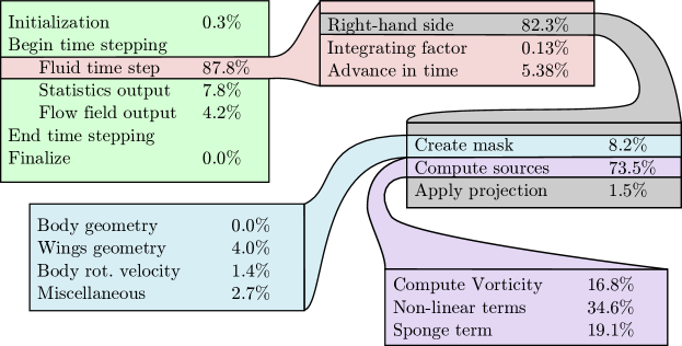
Figure 4: Partition of computational efforts spent on a bumblebee simulation (see section 6). The resolution is $1152\times 768\times 768$. Most efforts are spent on advancing the fluid in time, which in turn is largely dominated by the computation of fluid source terms. All per-cent is with respect to total execution time.

5 Validation Tests

For code validation we consider four test cases with increasing complexity, a falling sphere, a rectangular flapping wing, a hovering flight of a fruit fly and the free flight of a butterfly model.

5.1 Falling sphere

The first test case to validate the flow solver is the sedimentation of a sphere, which in our terminology is an insect without wings and with a spherical body. We consider case 1 proposed by Mordant and Pinton [23], who studied the sedimentation problem experimentally in a water tank. The sphere of unit diameter and mass $M=1.3404$ is falling in fluid of viscosity $\nu=0.0228$ and unit density. The dimensionless gravity is $g=0.8036$ and the terminal settling velocity obtained from the experiments is $U=0.9488$. We perform a grid convergence test using the domain size $8\times 8\times 16$, and parameters $N_{x}\times N_{y}\times N_{z}\times C_{\eta}$ of a coarse ($96\times 96\times 192\times 10^{-3}$), medium ($192\times 192\times 384\times 2.5\cdot 10^{-4}$) and fine ($384\times 384\times 768\times 6.25\cdot 10^{-5}$) grid. The number of points per penalization boundary layer is $K=0.0573$. The results of the convergence study are illustrated in figure 5 and the settling velocity for the finest resolution differs from the experimental findings by less than 1%. The finest resolution required 30 GB of memory and 34 400 CPU hours on 1024 cores to perform 266 667 time steps. The computational cost is relatively high, since small values of $C_{\eta}$ are required as the Reynolds number is small.

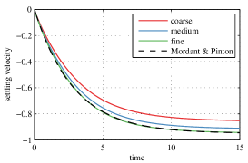
Figure 5: Settling velocity of a falling sphere, experimental results by Mordant & Pinton [23] and present results for coarse, medium and fine grids.

5.2 Validation case of a rectangular flapping wing

We consider the setup proposed by Suzuki and co-workers in [34] Appendix B2. It considers only one rectangular wing with a finite thickness, neglecting thus the body and the second wing. The fact that the thickness is finite and the geometry rather simple, compared to actual insects, motivates the choice of this setup. The wing kinematics are given by $\phi=\phi_{m}\cos\left(2\pi t\right)$, $\alpha=\frac{\alpha_{m}}{\tanh c_{\alpha}}\tanh\left(c_{\alpha}\sin\left(2\pi t\right)\right)$ and $\theta=0$, where $\phi_{m}=80^{\circ}$, $\alpha_{m}=45^{\circ}$, $c_{\alpha}=3.3$; the motion is symmetric for the up- and downstroke and depicted in figure 6 (a-b). The rectangular wing and the wing coordinate system are illustrated in figure 6 (c). We normalize the distance from pivot to tip to unity, which yields $a=1.6667$, $b=0.0667$, $B=0.4167$ and a wing thickness of $h=0.04171$. The Reynolds number is set to $\mathrm{Re}=U_{\mathrm{tip}}B/\nu=100$ with $U_{\mathrm{tip}}=2\pi\phi_{m}$, yielding the kinematic viscosity $\nu=0.0366$. In the present simulations, we discretize the domain of size $3\times 3\times 3$ using $512\times 512\times 512$ points and a penalization parameter of $C_{\eta}=1.25\cdot 10^{-4}$ ($K=0.365$). The reference computation in [34] is performed in a domain of size $4.16\times 4.16\times 4.16$, using a fine grid near the wing and a coarse one in the far-field. Based on the resolution of the fine grid, $\Delta x=B/50$, the corresponding equidistant resolution would be $500^{3}$. In our simulations, the body reference point is located at $\underline{x}_{\mathrm{cntr}}^{(g)}=(1.5,\,1.5,\,1.7)$ and coincides with the wing pivot point, thus $\underline{x}_{\mathrm{pivot}}^{(b)}=0$. The orientation of the body coordinate system is given by $\psi=0^{\circ}$, $\beta=-45^{\circ}$, $\gamma=45^{\circ}$ and $\eta=-45^{\circ}$, where the $45^{\circ}$ yaw angle was added to keep the wing as far away from the vorticity sponges as possible. A total of four strokes has been computed, starting with a quiescent initial condition, $\underline{u}\left(\underline{x},t=0\right)=0$. The outer boundary conditions on the domain are homogeneous Dirichlet conditions in $z$-direction and a vorticity sponge, extending over $32$ grid points with $C_{\mathrm{sp}}=10^{-1}$, in the remaining ones. The simulation required 35 GB of memory and 5785 CPU hours on 1024 cores. A total of 27 701 time steps was performed.

The resulting time series of the vertical force is illustrated in figure 6 (d). It takes the first two wingbeats to develop a periodic state, since the motion is impulsively started, and then the following strokes are almost identical. The present solution agrees well with the reference solution, and the relative R.M.S difference is $\left\|F-F_{\mathrm{ref}}\right\|_{2}/\left\|F_{\mathrm{ref}}\right\|_{2}\approx 4\%$ over the last two periods.

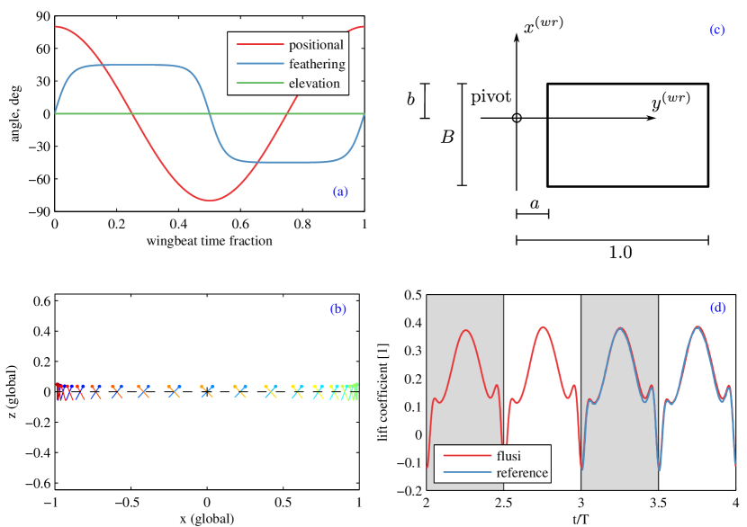
Figure 6: Flapping rectangular wing. (a) kinematics used in the test case, as given by Suzuki et al. [34]. (b) visualization of the wing kinematics by a chord section (without body, color represents time) (c) Geometry of the flapping rectangular wing. Contrary to [34], we normalize the distance pivot-wing tip to unity. (d) time evolution of the vertical force acting on the wing for the last two strokes, with the reference solution presented in [34].

5.3 Hovering flight of a fruit fly model

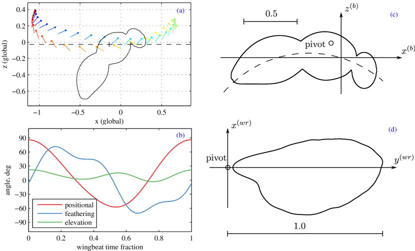
Figure 7: Hovering fruit fly, for comparison with [21]. (a): wingbeat kinematics in the side view. (b) time evolution of the wing angles. (c) Drawing of the insect’s body in the plane $y^{(b)}=0$. The body is rotationally symmetric with a circular center line. (d) Drawing of the wing shape, together with its pivot point.

The third validation test compares with a hovering fruit fly model, of which numerical simulations have been presented by Maeda and Liu [21]. Their simulations are based on overset grids, i.e., a body-fitted grid for the wings ($65\times 65\times 11$ each) and the body ($61\times 61\times 9$), as well as a background grid ($161\times 141\times 127$) have been used to solve the incompressible Navier–Stokes equations, approximated in the artificial compressibility formulation, using a finite volume discretization.

The fruit fly considered is defined in figure 7. The wing length from pivot point to wing tip, $R=2.47\,\mathrm{mm}$, the fluid density $\varrho_{f}=1.225\,\mathrm{kg/m^{3}}$ and the wingbeat frequency $f=218\,\mathrm{Hz}$ are used for normalization. The body, depicted in figure 7 (a,c), has an elliptical cross-section with center points following an arched centerline of radius $r_{\mathrm{bc}}=0.94644$ centered at $x_{\mathrm{bc}}^{(b)}=-0.244769$, $z_{\mathrm{bc}}^{(b)}=-0.9301256$. The wing pivot points are located at $\underline{x}_{\mathrm{pivot,rl}}^{(b)}=\left(-0.12,\,\pm 0.1445,\,0.08\right).$ To facilitate reproduction, the supplementary material contains STL files (StereoLithography) of the fruitfly geometry, as well the parameter file that can be used to reproduce the results with FluSI. The insect is tethered at $\underline{x}_{c}^{(g)}=\left(1.6,\,1.6,\,1.9\right)$ in a computational domain of size $3.2\times 3.2\times 3.2$, discretized with $640\times 640\times 640$ Fourier modes and a penalization parameter of $C_{\eta}=1.15\cdot 10^{-4}$ ($K=0.23$). Its body orientation is given by $\psi=0$, $\beta=-45^{\circ}$, $\gamma=45^{\circ}$ and $\eta=-45^{\circ}$. The fruit fly hovers, thus the body position and orientation do not change in time. A total of four wing beats has been computed, and the initial condition is fluid at rest, $\underline{u}\left(\underline{x},t=0\right)=\underline{0}$. We apply a vorticity sponge in the $x$ and $y$-direction ($32$ grid points thick with $C_{\mathrm{sp}}=10^{-1})$ and impose no-slip boundary conditions in the $z$-direction, i.e., we impose floor and ceiling. The simulation required 68 GB of memory and 15 100 CPU hours on 1024 cores. A total of 48 200 time steps was performed.

The wing shape is illustrated in figure 7 (d). It has a mean chord $c_{m}=A/R=0.33$, which yields with the kinematic viscosity of air, $\nu=1.5\cdot 10^{-5}\,\mathrm{m^{2}/s}$ the Reynolds number $\mathrm{Re}=U_{\mathrm{tip}}c_{m}/\nu=2\Phi Rfc_{m}/\nu=136$ where $\Phi=2.44\,\mathrm{rad}$ is the stroke amplitude of the positional angle. The time evolution of the wing kinematics is illustrated in figure 7 (b). The up- and downstroke are not symmetric, and the wing trajectory, figure 7 (a), shows the characteristic $\cup$-shape.

The results for the lift force, normalized with the weight, and the aerodynamic power in W/kg body mass are presented in figure 8. As the mass of the model insect was not given in [21], we assumed the fourth stroke of the reference data to balance the weight, yielding $m=1.02\,\mathrm{mg}$. Small circles at mid-stroke indicate stroke-averaged values. For the stroke-averaged vertical force, we find respectively $10.03\%$, $6.19\%$, $4.03\%$ and $3.26\%$ relative difference to the reference data for the four strokes computed, which can be explained by the impulsively started motion at the beginning of the first stroke. The time evolution, e.g., the occurrence of peaks, are very similar in both data sets. The agreement is even better for the aerodynamic power, with relative differences of $0.57\%$, $0.06\%$, $-0.95\%$ and $-1.00\%$ for the stroke-averaged values. Both power and lift peak during the translation phase of the up- and downstroke, and reach a minimum value at the reversals.

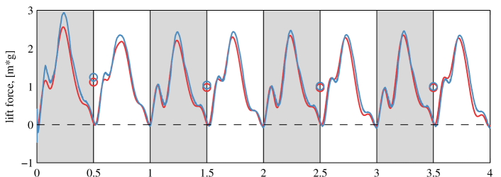
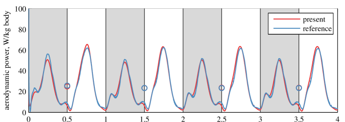
Figure 8: Hovering fruit fly, comparison with [21]. Top: total vertical force. Bottom: aerodynamic power. Gray shaded areas denote upstrokes, stroke averages are indicated by circles. The mean values during the last stroke differ by 3.26% and 1.00% for the vertical force and the power, respectively.

The flow field generated by the fruit fly model is visualized in figure 9 by iso-surfaces of the $Q$-criterion, which can, for incompressible flows, be computed as $Q=\nabla^{2}p/2$, see [18, p. 23]. The flow field exhibits the typical features, such as a leading edge vortex and a wingtip vortex.

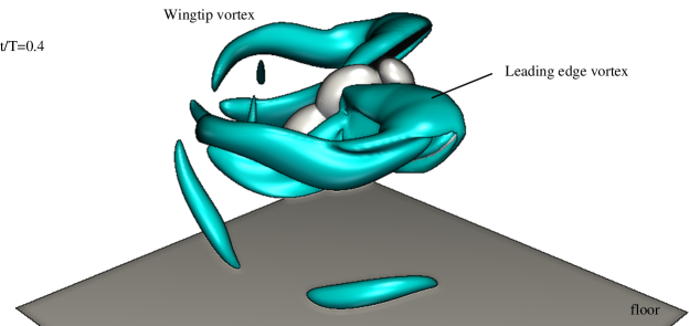
Figure 9: Snapshot of the vortical structures generated by a hovering fruit fly model, visualized by iso-surfaces of the $Q$-criterion ($Q=100$) shortly before the ventral stroke reversal $t/T=0.4$. Typical feature of flapping flight, such as the leading edge and wingtip vortex, are visible.

5.4 Butterfly model in free flight

To complete the validation section, we consider the freely flying butterfly model presented in [34, section 5.3]. The body consists of a thin rod with quadratic wings of length $R=1$, and the wing kinematics is inspired by a butterfly. Figure 10 (top row) illustrates the prescribed wingbeat kinematics, converted to the convention used in this work. The Reynolds number is $Re=300=U_{\mathrm{tip}}R/\nu$, where $U_{\mathrm{tip}}=\pi$ is the mean wingtip velocity. The mass of the butterfly is $M=38$, and the moments of inertia of the body are given by $J_{y}^{(b)}=J_{z}^{(b)}=3.1667$. The roll motion is inhibited (five degrees of freedom) and the mass of the wings is neglected. Gravitational acceleration is given by $g=0.1304$. Present computations are performed on a domain of size $6\times 6\times 6$ using a resolution of $1024\times 1024\times 1024$ and the penalization constant is $C_{\eta}=1.4\cdot 10^{-4}$ ($K=0.2$). We apply a vorticity sponge in all directions, centered around the moving center of the insect $\underline{x}_{\mathrm{cntr}}^{(g)}$. We computed 9 strokes (65066 time steps), the computation allocated $200$ GB of memory and consumed $79915$ CPU hours on $4096$ cores. The parameter files used in this compuation are in the supplementary material.

Figure 10 (mid row) compares the coordinates of the center of mass and the body pitch angle with the reference solution, showing good agreement with the reference computation. A slight deviation in the vertical component can be observed, which can be explained by the fact that the slight differences in the forces (Fig. 10 bottom row) are integrated twice with respect to time. The general agreement is good, and we conclude that our code is validated.

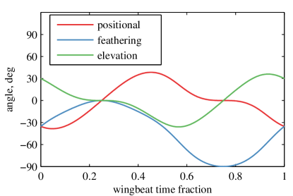
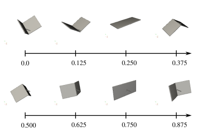
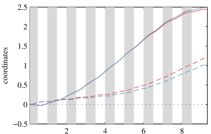
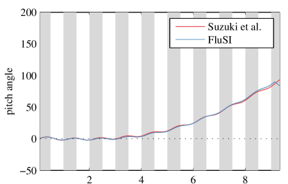
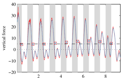
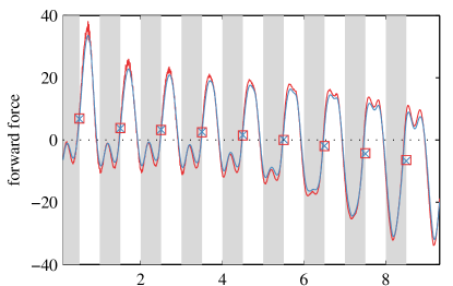
Figure 10: Freefly flying butterfly model for comparison with [34]. Top: kinematics and illustration of the wingbeat. Mid left: coordinates of the center of mass for the horizontal (solid lines) and vertical (dashed line) component. Mid right: body pitch angle $\beta$. Bottom: vertical (left) and forward force (right) component. Symbols indicate stroke averages. Dash-dotted line marks weight. Overall agreement is good.

6 Application to a bumblebee model in forward flight

In order to demonstrate the applicability of the software environment to more complex insects at higher Reynolds number, we consider in this chapter a different insect model with a Reynolds number of $\mathrm{Re}=2\Phi Rfc_{m}/\nu=2042$. The model is derived from a bumblebee and its detailed morphology and kinematics can be found in the supplementary material (STL file of the geometry as well as the parameter files that can be used to reproduce the results with FluSI). The model has also been used in [10, suppl. mat.]. The body contains details such as the legs and antennae, since they can be easily included in the present framework. The bumblebee is considered in forward flight at $u_{\infty}=1.246$. The domain size is set to $6\times 4\times 4$ and discretized with $1152\times 768\times 768$ grid points. The penalization parameter is set to $C_{\eta}=2.5\cdot 10^{-4}$ ($K=0.074$). Four strokes have been simulated, requiring $26467$ CPU hours on 1024 cores and 153.6 GB of memory.

Figure 11 visualizes the flow field generated by the model by the $\left\|\underline{\omega}\right\|=100$ isosurface of vorticity magnitude, for the times $t/T=0.3$ and $0.95$, where $T$ is the period time. At $t/T=0.3$, the leading edge vortex and the wingtip vortex are clearly visible, yet the flow field presents much smaller scales than in the case of a fruitfly (Fig. 9). At $t/T=0.95$, which is shortly before the beginning of a new cycle, the vortex “puff” shed at the stroke reversal ($t/T\approx 0.5$) are visible. The flow field is both spatially and temporally intermittent. Figure 11 gives the impression of a turbulent flow field, which can be quantified by the energy spectra of the velocity in a 2D slice perpendicular to the flow direction. Figure 12 shows the chosen position of the slice at $x=2.67$, and the radial energy spectra for 10 times throughout the cycle. At any time $t/T$, the energy spectrum $E(k)=1/2\sum_{k-1/2\leq|\underline{k}|<k+1/2}\left|\widehat{u}_{x}\left(\underline{k}\right)\right|{}^{2}+\left|\widehat{u}_{z}\left(\underline{k}\right)\right|^{2}+\left|\widehat{u}_{z}\left(\underline{k}\right)\right|^{2}$, where $\underline{k}=\left(k_{x},k_{y}\right)$, is full and exhibits an intertial range with a $k^{-5/3}$ slope, which is a typical feature of turbulence.

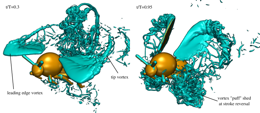
Figure 11: Flow field generated by the model bumblebee in forward flight, visualized by the $\left\|\underline{\omega}\right\|=100$ isosurface of vorticity magnitude.

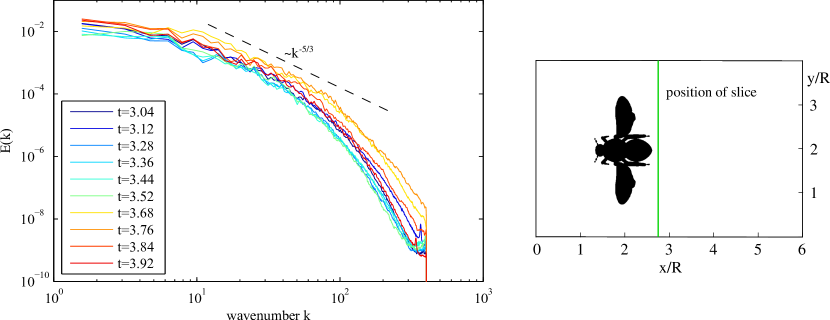
Figure 12: Right: Radial energy spectra in a slice perpendicular to the flow direction ($x=2.67$). The spectra are full and exhibit an inertial- and dissipative range. The resolution is $1152\times 768\times 768$, thus the highest resolved wavenumber is $k_{\mathrm{max}}=256\cdot\left(2\pi/4\right)$, due to the de-aliasing using the $2/3$ rule. Right: position of the slice and insect in the computational domain of size $6\times 4\times 4$.

As described in section 2.3, a vorticity sponge technique has been used to overcome the periodicity. Let us briefly discuss the influence of the sponge and the choice of parameters. Figure 13 visualizes the flow field from two simulations, one with a shorter domain ($4\times 4\times 4$) and the previously discussed one. In the shorter domain, a sponge is active in the region $3.5\leq x\leq 4$ with a constant of $C_{\mathrm{sp}}=10^{-1}$.

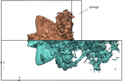
Figure 13: Influence of the vorticity sponge in a bumblebee simulation. Shown is the $\left\|\underline{\omega}\right\|=20$ isosurface of vorticity magnitude. A simulation with a longer ($\ell_{x}=6$, blue) and a shorter domain ($\ell_{x}=4$, orange) have been performed. In the shorter simulation, the sponge occupies the region $3.5\leq x\leq 4$. The sponge constant is $C_{\mathrm{sp}}=10^{-1}.$

7 Conclusions and Perspectives

This article presents the open source software FluSI (https://github.com/pseudospectators/FLUSI) for the numerical simulation of the aerodynamics of flapping insect flight running on massive parallel computer architectures. Different benchmarks demonstrated the efficiency of the code and showed its validity in comparison with results from the literature. The numerical method is based on a Fourier pseudo-spectral discretization of the three-dimensional incompressible Navier–Stokes equations. Thus no artificial numerical diffusion or dispersion are introduced in the discretization. The no-slip boundary conditions for the complexly shaped and time varying geometry of the flapping wings and the insect body are imposed with the volume penalization method. The penalization parameter is chosen such that the modeling error, due to penalization, and the discretization error are balanced. The computational cost of the flow solver is essentially due to the Fourier transforms. Benefiting from the efficient implementation of three-dimensional FFT, excellent scaling on large scale computing clusters has thus been obtained. A limitation of the current approach is that equidistant Cartesian grids are required and a compromize between the domain size and the number of grid points has to be imposed. The modular structure of the FluSI code permits to design different and complex geometries of the insect shape and its wings easily and also to change their kinematics. For the free flight option, equations in a quaternion-based formulation are solved. Different flow configurations, like channel flows with laminar or turbulent inflow or including bluff bodies of almost arbitrary shape, are possible using penalization together with a sponge technique.

References

- [1] P. Angot, C. Bruneau, and P. Fabrie, A penalization method to take into account obstacles in incompressible viscous flows, Numer. Math., 81 (1999), pp. 497–520.
- [2] E. Arquis and J.-P. Caltagirone, Sur les conditions hydrodynamiques au voisinage d’une interface milieu fluide milieu poreux: application à la convection naturelle, C. R. Acad. Sci. Paris, Sér. II, 299 (1984).
- [3] G. J. Berman and Z. J. Wang, Energy-minimizing kinematics in hovering insect flight, J. Fluid Mech., 582 (2007), pp. 153–168.
- [4] G. Bimbard, D. Kolomenskiy, O. Bouteleux, J. Casas, and R. Godoy-Diana, Force balance in the take-off of a pierid butterfly: relative importance and timing of leg impulsion and aerodynamic forces, J. Exp. Biol., 216 (2013), pp. 3551–3563.
- [5] C. Canuto, M. Y. Hussaini, A. Quarteroni, and T. Zang, Spectral Methods in Fluid Dynamics, Springer Verlag, 1986.
- [6] G. Carbou and P. Fabrie, Boundary layer for a penalization method for viscous incompressible flow, Adv. Diff. Equ., 8 (2003), pp. 1453–2480.
- [7] J. W. Cooley and J. W. Tukey, An algorithm for the machine calculation of complex Fourier series, Math. Comput., 19 (1965), pp. 297–301.
- [8] T. Engels, D. Kolomenskiy, K. Schneider, and J. Sesterhenn, Two-dimensional simulation of the fluttering instability using a pseudospectral method with volume penalization, Computers & Structures, 122 (2012), pp. 101–112.
- [9] T. Engels, D. Kolomenskiy, K. Schneider, and J. Sesterhenn, Numerical simulation of fluid-structure interaction with the volume penalization method, J. Comput. Phys., 281 (2015), pp. 96–115.
- [10] T. Engels, D. Kolomenskiy, K. Schneider, J. Sesterhenn, and F.-O. Lehmann, Bumblebee flight in heavy turbulence, Phys. Rev. Lett., accepted, (2015).
- [11] M. Frigo and S. G. Johnson, The design and implementation of FFTW3, Proc. IEEE, 94 (2005), pp. 216–231.
- [12] M. Hejlesen, P. Koumoutsakos, A. Leonard, and J. Walther, Iterative Brinkman penalization for remeshed vortex methods., J. Comput. Phys., 280 (2015), pp. 547–562.
- [13] C. Introini, M. Belliard, and C. Fournier, A second order penalized direct forcing for hybrid Cartesian/immersed boundary flow simulations, Computers & Fluids, 90 (2014), pp. 21–41.
- [14] C. Ji, A. Munjiza, and J. Williams, A novel iterative direct-forcing immersed boundary method and its finite volume applications, J. Comput. Phys., 231 (2012), pp. 1797–1821.
- [15] B. Kadoch, D. Kolomenskiy, P. Angot, and K. Schneider, A volume penalization method for incompressible flows and scalar advection-diffusion with moving obstacles, J. Comput. Phys., 231 (2012), pp. 4365–4383.
- [16] J. Kim and P. Moin, Application of a fractional-step method to incompressible navier-stokes equations, J. Comput. Phys., 59 (1985), pp. 308–323.
- [17] D. Kolomenskiy and K. Schneider, A Fourier spectral method for the Navier-Stokes equations with volume penalization for moving solid obstacles, J. Comput. Phys., 228 (2009), pp. 5687–5709.
- [18] M. Lesieur, O. Métais, and P. Comte, Large-Eddy Simulations of Turbulence, Cambridge University Press, 2005.
- [19] H. Liu, Integrated modeling of insect flight: From morphology, kinematics to aerodynamics, J. Comput. Phys., 228 (2009), pp. 439–459.
- [20] M. Maeda, N. Gao, N. Nishihashi, and H. Liu, A free-flight simulation of insect flapping flight, J. Aero Aqua Bio-mech., 1 (2010), pp. 71–79.
- [21] M. Maeda and H. Liu, Ground effect in fruit fly hovering: A three-dimensional computational study., J. Biomech. Sc. Engin., 8 (2013), pp. 344–355.
- [22] R. Mittal and G. Iaccarino, Immersed boundary methods, Annu. Rev. Fluid Mech., 37 (2005), pp. 239–261.
- [23] N. Mordant and J.-F. Pinton, Velocity measurement of a settling sphere, Eur. Phys. J. B, 18 (2000), pp. 343–352.
- [24] R. Nguyen van yen, D. Kolomenskiy, and K. Schneider, Approximation of the Laplace and Stokes operators with Dirichlet boundary conditions through volume penalization: A spectral viewpoint, Numer. Math., 128 (2014), pp. 301–338.
- [25] S. Osher and R. Fedkiw, Level Set Methods and Dynamic implicit Surfaces, Springer, 2003.
- [26] D. Pekurovsky, P3DFFT: a framework for parallel computations of Fourier transforms in three dimensions, SIAM J. Sci. Comput., 34 (2012), pp. C192–C209.
- [27] C. S. Peskin, The immersed boundary method, Acta Numerica, 11 (2002), pp. 479–517.
- [28] R. Peyret, Spectral Methods for Incompressible Viscous Flow, Springer Berlin / Heidelberg, 2002.
- [29] R. Ramamurti and W. Sandberg, A computational investigation of the three-dimensional unsteady aerodynamics of drosophila hovering and maneuvering, J. Exp. Biol., 210 (2009), pp. 881–896.
- [30] P. Schlatter, N. Adams, and L. Kleiser, A windowing method for periodic inflow/outflow boundary treatment of non-periodic flows, J. Comput. Phys., 206 (2005), pp. 505–535.
- [31] K. Schneider, Numerical simulation of the transient flow behaviour in chemical reactors using a penalisation method, Computers & Fluids, 34 (2005), pp. 1223–1238.
- [32] K. Schneider, Immersed boundary methods for numerical simulation of confined fluid and plasma turbulence in complex geometries: a review., J. Plasma Phys., 81 (2015), p. 435810601.
- [33] K. Schneider and M. Farge, Numerical simulation of the transient flow behaviour in tube bundles using a volume penalization method, J. Fluids Struct., 20 (2005), pp. 555–566.
- [34] K. Suzuki, K. Minami, and T. Inamuro, Lift and thrust generation by a butterfly-like flapping wing-body model: immersed boundary-lattice Boltzmann simulations, J. Fluid Mech., 767 (2015), pp. 659–695.
- [35] J. F. Thompson, Z. Warsi, and C. W. Mastin, Numerical grid generation: Foundations and Applications., North-Holland Amsterdam, 1985.
- [36] M. Uhlmann, An immersed boundary method with direct forcing for the simulation of particulate flows, J. Comput. Phys., 209 (2005), pp. 448–476.