$B^{*}B\pi$ coupling using relativistic heavy quarks

Abstract

We report on a calculation of the $B^{*}B\pi$ coupling in three-flavour lattice QCD. This coupling, defined from the strong-interaction matrix element $\langle B\pi|B^{*}\rangle$, is related to the leading order low-energy constant in heavy meson chiral perturbation theory (HM$\chi$PT). We carry out our calculation directly at the $b$-quark mass using a non-perturbatively tuned clover action that controls discretization effects of order $|\vec{p}a|$ and $(ma)^{n}$ for all $n$. Our analysis is performed on RBC/UKQCD gauge configurations using domain-wall fermions and the Iwasaki gauge action at two lattice spacings of $a^{-1}=1.729(25)\,\mathrm{GeV}$, $a^{-1}=2.281(28)\,\mathrm{GeV}$, and unitary pion masses down to $290\,\mathrm{MeV}$. We achieve good statistical precision and control all systematic uncertainties, giving a final result for the coupling $g_{b}=0.56(3)_{\mathrm{stat}}(7)_{\mathrm{sys}}$ in the continuum and at the physical light-quark masses. This is the first calculation performed directly at the physical $b$-quark mass and lies in the region one would expect from carrying out an interpolation between previous results at the charm mass and at the static point.

I Introduction

The power of lattice QCD in probing the Standard Model and uncovering evidence for new physics lies predominantly in the flavour sector. To constrain the Cabibbo–Kobayashi–Maskawa (CKM) unitarity triangle Charles et al. (2005); Bona et al. (2005); Laiho et al. (2010) requires many inputs that must be evaluated non-perturbatively, particularly in the $B$-meson sector. For instance, an important constraint on the apex of the CKM unitarity triangle comes from neutral $B$-meson mixing, which gives information on the ratio of CKM elements $|V_{ts}|^{2}/|V_{td}|^{2}$. Accessing these CKM elements from the experimental data requires knowledge of the $B$-meson decay constant and bag parameter, or alternatively the SU(3) breaking ratio

$$\frac{f_{B_{s}}\sqrt{B_{B_{s}}}}{f_{B_{d}}\sqrt{B_{B_{d}}}}.$$ (1)

Lattice calculations of the decay constants $f_{B_{d}}$ and $f_{B_{s}}$ are also necessary inputs for the Standard Model predictions of BR$(B\to\tau\nu)$ and BR$(B_{s}\to\mu^{+}\mu^{-})$ respectively, while lattice calculations of the $B\to\pi l\nu$ form factor allow a determination of the CKM matrix element $|V_{ub}|$. For both semileptonic form factors and mixing matrix elements, the precision of lattice calculations lags behind experiment. The experimental measurements will continue to improve with the large data sets available at Belle II and from LHCb. Therefore it is essential to reduce further the theoretical uncertainties in the non-perturbative hadronic parameters in order to maximise the scientific impact of current and future $B$-physics experiments.

A major source of uncertainty in all previous lattice calculations is from practical difficulties simulating at physical light-quark masses. Theoretical insight from HM$\chi$PT can guide extrapolations down to the physical point, but lack of knowledge of the low-energy constants (LECs) of the theory introduces uncertainties. For example, at next-to-leading order (NLO) in HM$\chi$PT and lowest order in the heavy-quark expansion the logarithmic dependence of $f_{B_{d}}$ and $B_{B_{d}}$ on the light-quark (or equivalently, pion) mass is given by Goity (1992); Sharpe and Zhang (1996)

$$f_{B_{d}} =F\left(1-\frac{3}{4}\frac{1+3\hat{g}^{2}}{(4\pi f_{\pi})^{2}}M_{\pi}^{2}\log(M_{\pi}^{2}/\mu^{2})\right)+\cdots,$$ (2)

$$B_{B_{d}} =B\left(1-\frac{1}{2}\frac{1-3\hat{g}^{2}}{(4\pi f_{\pi})^{2}}M_{\pi}^{2}\log(M_{\pi}^{2}/\mu^{2})\right)+\cdots,$$ (3)

where $\hat{g}$ is the leading-order LEC. The strong-interaction matrix element $\langle B\pi|B^{*}\rangle$ is used to determine a coupling $g_{b}$, which would become $\hat{g}$ in the static limit of an infinitely heavy $b$ quark. At the order used above in Eqs. (2) and (3), we are free to use $g_{b}$ in place of $\hat{g}$; differences between the two are of order $1/m_{b}$.

In this paper we perform the first calculation of the coupling $g_{b}$ directly at the $b$-quark mass. Previous determinations of the coupling have been hindered by the difficulties of simulating heavy quarks on the lattice. Lattice calculations have been performed for $g_{c}$, the analogous coupling for $D$-mesons Abada et al. (2002, 2004); Bećirević and Sanfilippo (2013); Can et al. (2013), and for $\hat{g}$ itself de Divitiis et al. (1998); Abada et al. (2004); Ohki et al. (2008); Detmold et al. (2012a); Bernardoni et al. (2015). Having a reliable theoretical calculation of the coupling for the $B$ system is important since this coupling cannot be accessed directly through experiment. The strong coupling $g_{D^{*}D\pi}$ has been measured by the CLEO collaboration Ahmed et al. (2001); Anastassov et al. (2002) and more recently by BaBar Lees et al. (2013a, b), but with $B$-mesons there is not enough phase-space for the $B^{*}\rightarrow B\pi$ decay to occur. Model estimates exist for $g_{b}$, including from QCD sum rules Colangelo et al. (1994); Belyaev et al. (1995); Dosch and Narison (1996); Colangelo and De Fazio (1998) and non-relativistic quark models Yan et al. (1992).

The rest of this paper is organised as follows. In section II we briefly review the framework of HM$\chi$PT, show how $g_{b}$ enters and present the method for extracting $g_{b}$ from lattice matrix-element calculations. Section III describes the parameters of the light-quark, gluon, and heavy-quark actions used in the numerical calculation and presents the ratios of two- and three-point correlators used to obtain $g_{b}$. In section IV we fit the correlator ratios to extract $g_{b}$ and then extrapolate these results to the continuum and physical quark masses using SU(2) HM$\chi$PT. We estimate the systematic errors in $g_{b}$ in section V, discussing each source of uncertainty in a different subsection. We conclude in section VI by presenting our final results and error budget, and comparing our result to other similar calculations.

II Heavy Meson Chiral Perturbation Theory

In the infinite heavy-quark mass limit the properties of heavy-light mesons become independent of the heavy quark’s spin and flavour quantum numbers. Combining this with the chiral symmetry present in the massless light-quark ($m_{q}\rightarrow 0$) limit of QCD provides the basis for heavy meson chiral perturbation theory. This effective theory of QCD is a joint expansion in powers of the inverse heavy-quark mass $1/m_{Q}$ and the light-quark-mass $m_{q}$.

In HM$\chi$PT the heavy-light pseudoscalar and vector mesons, $P$ and $P^{*}$, are combined in a covariant $4\times 4$ matrix representation

$$H=\frac{1+\not{v}}{2}\left(P^{*}_{\mu}\gamma^{\mu}-P\gamma_{5}\right).$$ (4)

If one includes three light dynamical quark flavors ($u,d,s$), this corresponds to SU(3) HM$\chi$PT with the usual octet of pseudo-Nambu-Goldstone bosons for the light pseudoscalars:

$$\mathcal{M}=\left(\begin{array}[]{ccc}\frac{1}{\sqrt{2}}\pi^{0}+\frac{1}{\sqrt{6}}\eta&\pi^{+}&K^{+}\\ \pi^{-}&-\frac{1}{\sqrt{2}}\pi^{0}+\frac{1}{\sqrt{6}}\eta&K^{0}\\ K^{-}&\bar{K}^{0}&-\sqrt{\frac{2}{3}}\eta\end{array}\right).$$ (5)

Because the strange-quark mass is almost thirty times larger than the average up-down quark mass, however, one can also treat the strange quark as heavy and include only the up- and down-quark dynamical degrees of freedom; this leads to SU(2) HM$\chi$PT (with the corresponding modification of $\mathcal{M}$). At lowest order the interactions between the heavy and light mesons are determined by a Lagrangian with a single LEC Wise (1992); Casalbuoni et al. (1997)

$$\mathcal{L}_{\mathrm{HM}\chi\mathrm{PT}}^{\mathrm{int}}=\hat{g}\,\mathrm{Tr}(\bar{H}_{a}H_{b}\mathcal{A}_{ba}^{\mu}\gamma_{\mu}\gamma_{5}),$$ (6)

where

$$\mathcal{A}_{\mu}=\frac{i}{2}\left(\xi^{\dagger}\partial_{\mu}\xi-\xi\partial_{\mu}\xi^{\dagger}\right)$$ (7)

and $\xi=\exp(i\mathcal{M}/f_{\pi})$. The roman indices run over light-quark flavour and the trace is over Dirac indices. We use a convention where $f_{\pi}\approx 130\,\mathrm{MeV}$.

The matrix element for the strong transition $B^{*}\rightarrow B\pi$ is parametrised by $g_{B^{*}B\pi}$,

$$\langle B(p^{\prime})\pi(q)|B^{*}(p,\lambda)\rangle=g_{B^{*}B\pi}\;q\cdot\epsilon^{(\lambda)}(p),$$ (8)

where $q=p-p^{\prime}$ and $\epsilon^{(\lambda)}(p)$ is the polarization vector for polarization state labelled by $\lambda$. Evaluating the same matrix element at leading order in HM$\chi$PT,

$$\langle P(p^{\prime})\pi(q)|P^{*}(p,\lambda)\rangle=\frac{2M_{P}}{f_{\pi}}\hat{g}\;q\cdot\epsilon^{(\lambda)}(p),$$ (9)

enables the determination of $g_{b}$ from

$$g_{B^{*}B\pi}=\frac{2M_{B}}{f_{\pi}}g_{b},$$ (10)

with $g_{b}$ equal to $\hat{g}$ up to $1/m_{b}^{n}$ corrections.

Performing a Lehmann–Symanzik–Zimmermann reduction and using the partially-conserved axial current relation for a soft pion, Eq. (8) becomes

$$g_{B^{*}B\pi}\;q\cdot\epsilon^{(\lambda)}(p)=\\ iq_{\mu}\frac{M_{\pi}^{2}-q^{2}}{f_{\pi}M_{\pi}^{2}}\int d^{4}x\;e^{iq\cdot x}\langle B(p^{\prime})|A^{\mu}(x)|B^{*}(p,\lambda)\rangle,$$ (11)

where $A^{\mu}=\bar{\psi}_{1}\gamma^{\mu}\gamma_{5}\psi_{2}$ is the light-quark axial-vector current. Using a form-factor decomposition of the matrix element

$$\langle B(p^{\prime})|A^{\mu}|B^{*}(p,\lambda)\rangle=2M_{B^{*}}A_{0}(q^{2})\,\frac{\epsilon^{(\lambda)}\cdot q}{q^{2}}q^{\mu}\\ \begin{aligned} &+(M_{B^{*}}+M_{B})A_{1}(q^{2})\left[\epsilon^{(\lambda)\mu}-\frac{\epsilon^{(\lambda)}\cdot q}{q^{2}}q^{\mu}\right]\\ &+A_{2}(q^{2})\,\frac{\epsilon^{(\lambda)}\cdot q}{M_{B^{*}}{+}M_{B}}\left[p^{\mu}+p^{\prime\mu}-\frac{M_{B^{*}}^{2}{-}M_{B}^{2}}{q^{2}}q^{\mu}\right],\end{aligned}$$ (12)

we see that at $q^{2}=0$

$$g_{B^{*}B\pi}=\frac{2M_{B^{*}}A_{0}(0)}{f_{\pi}}.$$ (13)

On the lattice, we cannot simulate exactly at $q^{2}=0$ without using twisted boundary conditions. Furthermore and from Eq. (11), we see that the form factor $A_{0}$ contains a pole at the pion mass, so it will be difficult to do a controlled extrapolation to $q^{2}=0$. However, the decomposition in Eq. (12) must be free of unphysical poles, which allows us to obtain the relation

$$g_{B^{*}B\pi}=\frac{1}{f_{\pi}}\left[(M_{B^{*}}+M_{B})A_{1}(0)+(M_{B^{*}}-M_{B})A_{2}(0)\right].$$ (14)

The $A_{1}$ term is expected to dominate because the relative contribution of $A_{2}$ is suppressed by the ratio $(M_{B^{*}}-M_{B})/(M_{B^{*}}+M_{B})$ whose value is $0.004$ for the physical $B$ and $B^{*}$ masses. It is this relation that we use for our numerical calculation.

III Calculational Strategy

III.1 Light quarks and gauge fields

Our analysis is carried out using ensembles produced by the RBC and UKQCD collaborations Allton et al. (2008); Aoki et al. (2011) with the Iwasaki gauge action Iwasaki (1983); Iwasaki and Yoshié (1984) and $2{+}1$ flavour dynamical domain-wall fermions Kaplan (1992); Shamir (1993). The configurations are at two lattice spacings, the finer $32^{2}$ ensembles have an inverse lattice spacing of $a^{-1}=2.281(28)\,\mathrm{GeV}$ and the coarser $24^{3}$ ensembles have $a^{-1}=1.729(25)\,\mathrm{GeV}$, corresponding to approximately $0.086\,\mathrm{fm}$ and $0.11\,\mathrm{fm}$ respectively. All ensembles have a spatial extent of $2.6\,\mathrm{fm}$. We simulate with unitary light-quarks corresponding to pion masses down to $M_{\pi}=289\,\mathrm{MeV}$. On all ensembles the strange sea-quark mass is tuned to within 10% of its physical value. The fifth dimensional extent of both lattices is $L_{S}=16$, corresponding to a residual quark mass of $m_{\mathrm{res}}a=0.003152$ on the $24^{3}$ ensembles and $m_{\mathrm{res}}a=0.0006664$ on the $32^{3}$ ensembles. The lattice quark masses corresponding to the physical $u/d$ and $s$ quarks are $\tilde{m}_{u/d}a=0.00136(4)$, $\tilde{m}_{s}a=0.0379(11)$ on the $24^{3}$ ensembles and $\tilde{m}_{u/d}a=0.00102(5)$, $\tilde{m}_{s}a=0.0280(7)$ on the $32^{3}$ ensembles. The tildes indicate that these values include the residual quark mass.

Our calculation makes use of unitary light-quark propagators with point sources previously generated as part of the RBC/UKQCD $B$-physics program Aoki et al. (2012); Witzel (2012); Christ et al. (2015); Kawanai et al. (2012); Flynn et al. (2015). Full details of the ensembles and propagators used are presented in Table 1. We perform a random translation on each gauge field configuration to minimise the effects of autocorrelations on our results, allowing us to use more closely spaced trajectories and gain statistics. For each configuration in the $32^{3}$ ensembles we use propagators computed at two time sources separated by half the lattice temporal extent to compensate for the smaller ensemble sizes.

Table 1: Lattice simulation parameters. All ensembles are generated using $2{+}1$ flavours of domain-wall fermions and the Iwasaki gauge action. All valence pion masses are equal to the sea-pion mass.

$L/a$	$a/\,\mathrm{fm}$	$m_{l}a$	$m_{s}a$	# configs	# sources	$M_{\pi}/\,\mathrm{MeV}$
24	0.11	0.005	0.04	1636	1	329
24	0.11	0.010	0.04	1419	1	419
24	0.11	0.020	0.04	345	1	558
32	0.08	0.004	0.03	628	2	289
32	0.08	0.006	0.03	889	2	345
32	0.08	0.008	0.03	544	2	394

III.2 Bottom quarks

Simulating heavy quarks on the lattice presents the problem of dealing with $m_{Q}a\geq 1$. A number of approaches have been developed to tackle this problem. In the limit of infinite mass the quarks become a static source of colour charge and their lattice propagator reduces to a trace of a product of temporal gauge links. This is the static action of Eichten and Hill Eichten and Hill (1990) which has been used extensively to calculate the coupling $g_{\infty}$, most recently in Detmold et al. (2012b); Bernardoni et al. (2015). Another approach is nonrelativistic QCD Lepage (1992), where the usual QCD Lagrangian is expanded in powers of $v/c$.

Here we use the relativistic heavy-quark (RHQ) action El-Khadra et al. (1997); Aoki et al. (2003); Christ et al. (2007) to simulate fully relativistic bottom quarks while controlling discretization effects. Although $m_{Q}a$ is large for the heavy quark in a heavy-light meson, the spatial momentum $|\vec{p}a|$ is of $O(a\Lambda_{\mathrm{QCD}})$. The RHQ action is an anisotropic Wilson action with a Sheikholeslami-Wohlert term Sheikholeslami and Wohlert (1985)

$$S_{\mathrm{RHQ}}=a^{4}\sum_{x,y}\bar{\psi}(y)\bigg{(}m_{0}+\gamma_{0}D_{0}+\zeta\vec{\gamma}\cdot\vec{D}-\frac{a}{2}(D_{0})^{2}-\frac{a}{2}\zeta(\vec{D})^{2}+\sum_{\mu\nu}\frac{ia}{4}c_{p}\sigma_{\mu\nu}F_{\mu\nu}\bigg{)}_{y,x}\psi(x).$$ (15)

El-Khadra, Kronfeld and Mackenzie showed that, for correctly tuned parameters, the anisotropic Clover action can be used to describe heavy quarks with controlled cut-off effects to all orders in $m_{Q}a$ and of $O(|\vec{p}a|)$ El-Khadra et al. (1997). Christ, Li, and Lin Christ et al. (2007) later showed that only three independent parameters need to be determined and, further, presented a method for performing this parameter tuning non-perturbatively Lin and Christ (2007).

This tuning has been completed for $b$ quarks Aoki et al. (2012) on the RBC/UKQCD configurations and those results (Table 2) are exploited in this calculation. The heavy-quark propagators and the correlation functions used in this analysis are calculated using the Chroma software library Edwards and Joo (2005). We apply Gaussian smearing to the heavy-quark propagators using parameters tuned in Aoki et al. (2012). Because the correlators become very small at large time separations owing to the large masses in the exponentials, we run the inverter for the heavy quark propagators to a very small relative residual ($10^{-45}$). We found that pursuing the conjugate gradient iteration to this small residual is equivalent to demanding convergence separately for the residual on each time slice.

Table 2: Tuned RHQ parameters for $b$ quarks from Ref. Aoki et al. (2012). The uncertainties shown are statistical, heavy-quark discretization effects, lattice-scale uncertainty, and from experimental inputs (the spin-averaged $B_{s}$-meson mass and $B_{s}$ hyperfine splitting) respectively.

$a/\,\mathrm{fm}$	$m_{0}a$	$c_{p}$	$\zeta$
0.11	8.45(6)(13)(50)(7)	5.8(1)(4)(4)(2)	3.10(7)(11)(9)(0)
0.08	3.99(3)(6)(18)(3)	3.57(7)(22)(19)(14)	1.93(4)(7)(3)(0)

III.3 Three-point correlation functions

Figure 1: Quark flow diagram

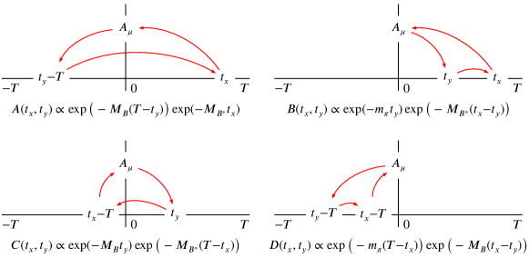
The matrix element that we wish to calculate in Eq. (12) corresponds to the quark-flow diagram shown in Fig. 1. To fully benefit from the available pre-calculated light-quark propagators, we arrange the calculation so that the axial-vector current is positioned at the light-quark propagator’s source. This means that we use the periodicity of the lattice, creating the $B^{*}$ meson at large time $t_{x}$, propagating to the origin at $t=0$, where the current acts and continuing to small time $t_{y}$, where the $B$-meson is annihilated. With this setup, we need only one inversion, a heavy-quark propagator calculated from $t_{y}$, using a light-quark propagator for the sequential source. The necessary trace is

$$C_{\mu\nu}^{(3)}\left(t_{x},t_{y};\vec{p},\vec{p}^{\prime}\right)=\\ \sum_{\vec{x},\vec{y}}e^{-i\vec{p}\cdot\vec{x}-i\vec{p}^{\prime}\cdot\vec{y}}\,\mathrm{Tr}\left[S_{l}(0,y)\gamma_{5}S_{h}(y,x)\gamma_{\nu}S_{l}(x,0)\gamma_{\mu}\gamma_{5}\right].$$ (16)

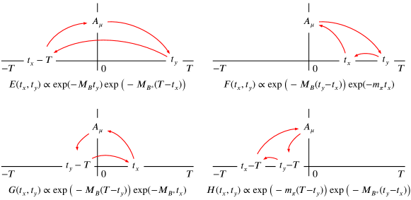
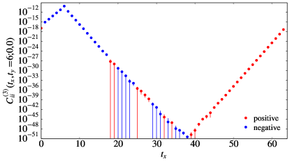
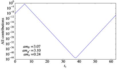
Because of the periodicity of the lattice there are further possible contributions beyond the desired Wick contraction in Fig. 1. An operator located at time $t$ can also be considered at location $t-T$, where $T$ is the lattice’s temporal extent. If we take into account separately the cases where $t_{x}>t_{y}$ and $t_{x}\leq t_{y}$, there are eight possible contributing arrangements (considering $t+nT$ for integer $n$ gives further contributions, but for increasing $|n|$ these are more and more suppressed). These are shown in Fig. 2. Using the approximation that the ground states immediately dominate the time dependence and that the matrix elements are all unity, we can estimate the time dependence of the three-point correlation function:

$$C^{(3)}(t_{x},t_{y})=\\ \begin{cases}A(t_{x},t_{y})+B(t_{x},t_{y})+C(t_{x},t_{y})+D(t_{x},t_{y})&t_{x}>t_{y},\\ E(t_{x},t_{y})+F(t_{x},t_{y})+G(t_{x},t_{y})+H(t_{x},t_{y})&t_{x}\leq t_{y}.\end{cases}$$ (17)

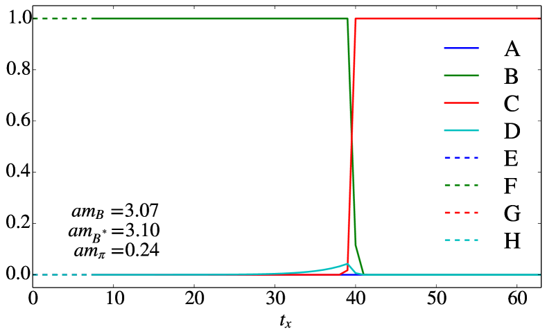
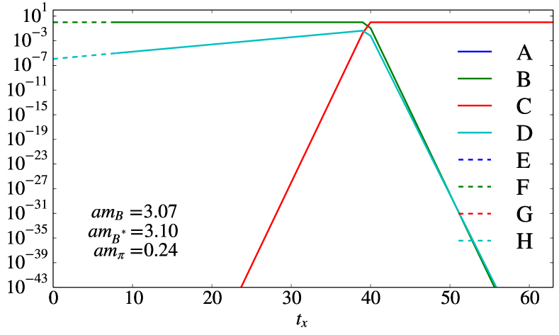
It is expected that the signal from which to extract the $B^{*}B\pi$ coupling will be seen at large $t_{x}$ (approaching $T$ from below), coming from the contribution shown as $C(t_{x},t_{y})$ in Fig. 2. Figure 3 shows the relative size of the different contributions as a function of $t_{x}$ with all matrix elements set to unity. As anticipated, $C$ is the dominant contribution in a region $T/2+t_{y}<t_{x}<T$. This result appears steady for a range of the masses $M_{B},M_{B^{*}},M_{\pi}$. Plotting the sum of the contributions as a function of $t_{x}$ (setting all matrix elements to unity) we see a peak at $t_{x}=t_{y}$ and an overall cosh-like form shifted by $t_{y}$ as shown on the right in Fig. 4. On the left of Fig. 4 we show good agreement with this form for our numerical data, with $t_{y}$ the time-position of the source for the sequential inversion. This gives us confidence that we can extract the desired matrix element from the large $t_{x}$ region of the three-point correlator.

Figure 2: Leading contributions to the three-point correlator for $t_{x}>t_{y}$ ($A,B,C,D$) and $t_{x}\leq t_{y}$ ($E,F,G,H$).

Figure 3: The estimated relative sizes, with $t_{y}=8$, of the eight contributions to the $B^{*}B\pi$ three-point function arising from different Wick contractions, using a linear scale (top) and log scale (bottom). Each contribution is scaled by dividing by the maximum contribution at that time. The matrix element of interest comes from $C$ which is shown as a solid red line on both plots. This contribution dominates for large $t_{x}$.

Figure 4: The three-point correlator of Eq. (18) evaluated on the $24^{3}$, $m_{l}a=0.005$ ensemble with $t_{y}=6$ (left). The time dependence closely matches that predicted from the analysis in Sec. III.3 (right).

III.4 Ratios

To access the matrix element in Eq. (12) we calculate the lattice three-point function

$$C_{\mu\nu}^{(3)}\left(t_{x},t_{y};\vec{p},\vec{p}^{\prime}\right)=\sum_{\vec{x},\vec{y}}e^{-i\vec{p}\cdot\vec{x}}e^{-i\vec{p}^{\prime}\cdot\vec{y}}\langle B(y)A_{\nu}(0)B_{\mu}^{*}(x)\rangle\overset{\begin{subarray}{c}T-t_{x}>0\\ t_{y}>0\end{subarray}}{\approx}\sum_{\lambda}\frac{Z_{B}^{1/2}Z_{B^{*}}^{1/2}}{2E_{B}2E_{B^{*}}}\langle B(p^{\prime})|A_{\nu}|B^{*}(p,\lambda)\rangle\epsilon^{(\lambda)}_{\mu}e^{-E_{B}t_{y}-E_{B^{*}}(T-t_{x})}$$ (18)

and the vector and pseudoscalar two-point functions

$$C_{BB}^{(2)}\left(t;\vec{p}\right) =\sum_{\vec{x}}e^{-i\vec{p}\cdot\vec{x}}\langle B(x)B(0)\rangle\approx Z_{B}\frac{e^{-E_{B}t}}{2E_{B}},$$ (19)

$$C_{B^{*}_{\mu}B^{*}_{\nu}}^{(2)}\left(t;\vec{p}\right) =\sum_{\vec{x}}e^{-i\vec{p}\cdot\vec{x}}\langle B^{*}_{\nu}(x)B^{*}_{\mu}(0)\rangle$$

$$\approx Z_{B^{*}}\frac{e^{-E_{B^{*}}t}}{2E_{B^{*}}}\left(\delta_{\mu\nu}-\frac{p_{\mu}p_{\nu}}{p^{2}},\right).$$ (20)

If we set both the vector and pseudoscalar momenta to zero in Eq. (18), such that $\vec{q}=\vec{p}=\vec{p}^{\prime}=0$ and $q^{2}=q_{0}^{2}=(M_{B^{*}}-M_{B})^{2}\approx 0$, we can see from Eq. (12) that the only form factor accessible is $A_{1}$. Hence we form the ratio (not summed on $i$):

$$R_{1}(t_{x},t_{y}) =\frac{C_{ii}^{(3)}(t_{x},t_{y};\vec{p}=0,\vec{p}^{\prime}=0)\,Z_{B}^{1/2}Z_{B^{*}}^{1/2}}{C_{BB}^{(2)}(t_{y};\vec{p}=0)\,C_{B^{*}_{i}B^{*}_{i}}^{(2)}(T-t_{x};\vec{p}=0)}$$

$$=(M_{B^{*}}+M_{B})A_{1}(q_{0}^{2}),$$ (21)

where we can average over the three spatial directions ($i=1,2,3$). To access the other form factors we need to inject a unit of momentum, such that $\vec{q}=\vec{p}=(1,0,0)\times 2\pi/L$ and $\vec{p}^{\prime}=0$. Following Abada et al. (2002), we define the ratios:

$$R_{2}(t_{x},t_{y}) =\frac{C_{10}^{(3)}(t_{x},t_{y};\vec{p}\neq 0,\vec{p}^{\prime}=0)\,Z_{B}^{1/2}Z_{B^{*}}^{1/2}}{C_{BB}^{(2)}(t_{y};\vec{p}^{\prime}=0)\,C_{B^{*}_{2}B^{*}_{2}}^{(2)}(T-t_{x};\vec{p}\neq 0)}$$

$$=\sum_{\lambda}\langle B(p^{\prime})|A_{0}|B^{*}(p,\lambda)\rangle\epsilon_{1}^{(\lambda)},$$ (22)

$$R_{3}(t_{x},t_{y}) =\frac{C_{11}^{(3)}(t_{x},t_{y};\vec{p}\neq 0,\vec{p}^{\prime}=0)\,Z_{B}^{1/2}Z_{B^{*}}^{1/2}}{C_{BB}^{(2)}(t_{y};\vec{p}^{\prime}=0)\,C_{B^{*}_{2}B^{*}_{2}}^{(2)}(T-t_{x};\vec{p}\neq 0)}$$

$$=\sum_{\lambda}\langle B(p^{\prime})|A_{1}|B^{*}(p,\lambda)\rangle\epsilon_{1}^{(\lambda)},$$ (23)

$$R_{4}(t_{x},t_{y}) =\frac{C_{22}^{(3)}(t_{x},t_{y};\vec{p}\neq 0,\vec{p}^{\prime}=0)\,Z_{B}^{1/2}Z_{B^{*}}^{1/2}}{C_{BB}^{(2)}(t_{y};\vec{p}^{\prime}=0)\,C_{B^{*}_{2}B^{*}_{2}}^{(2)}(T-t_{x};\vec{p}\neq 0)}$$

$$=\sum_{\lambda}\langle B(p^{\prime})|A_{2}|B^{*}(p,\lambda)\rangle\epsilon_{2}^{(\lambda)}$$

$$=(M_{B^{*}}+M_{B})A_{1}(q^{2}).$$ (24)

These allow access to the form factor $A_{2}$ through

$$\frac{A_{2}}{A_{1}}=\frac{(M_{B^{*}}+M_{B})^{2}}{2M_{B}^{2}q_{1}^{2}}\Bigg{[}-q^{2}_{1}+E_{B^{*}}(E_{B^{*}}-M_{B})\\ -\frac{M_{B^{*}}^{2}(E_{B^{*}}-M_{B})}{E_{B^{*}}}\frac{R_{3}}{R_{4}}-i\frac{M_{B^{*}}^{2}q_{1}}{E_{B^{*}}}\frac{R_{2}}{R_{4}}\Bigg{]}.$$ (25)

The ratio in Eq. (25) is obtained at non-zero values of $q^{2}$ and needs to be extrapolated to $q^{2}=0$. However, from Eq. (14) the contribution of $A_{2}(0)$ relative to $A_{1}(0)$ is suppressed by the ratio $(M_{B^{*}}-M_{B})/(M_{B^{*}}+M_{B})$. The form factor $A_{1}$ is obtained at $q_{0}^{2}=(M_{B^{*}}-M_{B})^{2}$ from Eq. (21), but examination shows that the slight extrapolation to $q^{2}=0$ is not necessary at the resolution possible with the available statistics. If we define functions $G_{1}$ and $G_{2}$

$$\begin{split}G_{1}(q^{2})&=(M_{B^{*}}+M_{B})A_{1}(q^{2}),\\ G_{2}(q^{2})&=(M_{B^{*}}-M_{B})A_{2}(q^{2}),\end{split}$$ (26)

we can write the coupling as $G_{1}(0)$ plus a small correction from the ratio $G_{2}/G_{1}$,

$$g_{b}=\frac{Z_{A}}{2M_{B}}G_{1}(0)\left(1+\frac{G_{2}(0)}{G_{1}(0)}\right),$$ (27)

where $Z_{A}$ is the light axial-vector current renormalization factor. In our simulations $A_{2}$ is of comparable size to $A_{1}$. The mass suppression in the ratio $G_{2}/G_{1}$ means that the correction term in (27) is at most $2\%$ on our ensembles and typically at the sub percent level, with an error comparable to its size.

We take $Z_{A}$ from the RBC/UKQCD combined analysis of the light hadron spectrum, pseudoscalar meson decay constants and quark masses on the $24^{3}$ and $32^{3}$ ensembles Aoki et al. (2011). The values are calculated from the ratio of the conserved and local vector currents, extrapolated to the chiral limit and are shown in Table 3.

Table 3: Axial current renormalization factors used in this work, calculated in Aoki et al. (2011).

Ensemble	$a/\mathrm{fm}$	$Z_{A}$
$24^{3}$	0.11	0.7019(26)
$32^{3}$	0.086	0.7396(17)

IV Analysis

IV.1 Correlator fits

Figure 5: The ratio $R_{1}(t,t_{y})$ evaluated for different values of $t_{y}$ on the $24^{3}$, $m_{l}a=0.005$ ensemble. $t_{y}=6$ gives the cleanest signal and longest plateau. The points for different $t_{y}$ have small horizontal offsets to help distinguish them on the plot.

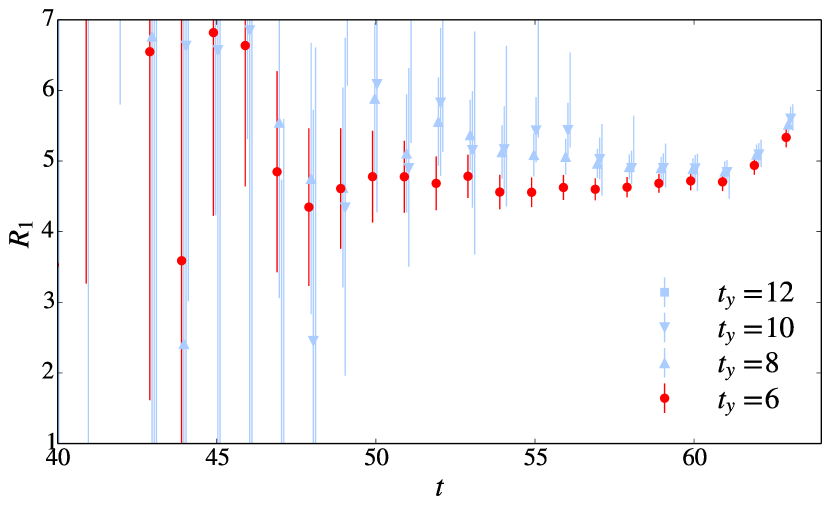
We first calculate the three-point function on the $24^{3}$ ensemble with $am_{l}=0.005$ for values of $t_{y}$ ranging from $6$ to $18$. Examining the data for $R_{1}$ (see Fig. 5), it is clear that the best signal is achieved with $t_{y}=6$. We therefore choose $t_{y}=6$ for our analysis on the $24^{3}$ ensembles and $t_{y}=8$ on the $32^{3}$ ensembles because it corresponds to the same physical distance.

Figure 6: Ratios $R_{1}(t,t_{y})$, $R_{2}(t,t_{y})$, $R_{3}(t,t_{y})$ and $R_{4}(t,t_{y})$ for $t_{y}=6$ on the $24^{3}$, $m_{l}a=0.005$ ensemble. $R_{1}$ is calculated with $\vec{p}=\vec{p}^{\prime}=0$, the other ratios with $\vec{p}=(1,0,0,0)2\pi/L$, $\vec{p}^{\prime}=0$.

Figure 7: $B$-meson (left) and $B^{*}$-meson (right) effective masses on the $24^{3}$, $m_{l}a=0.005$ ensemble.

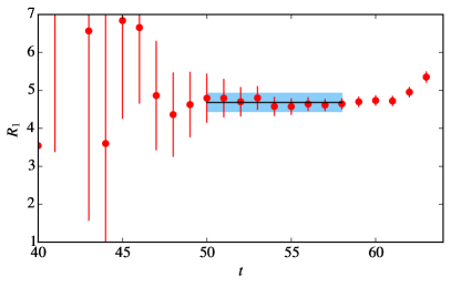
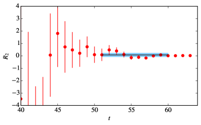
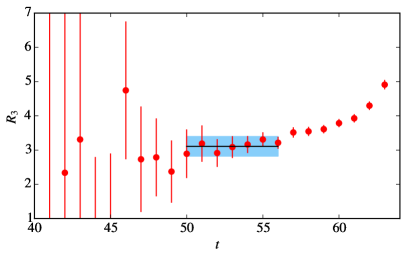
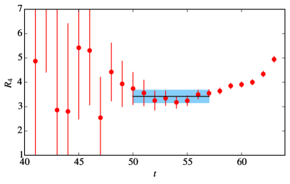
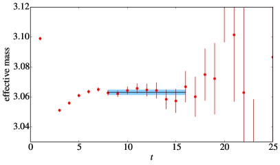
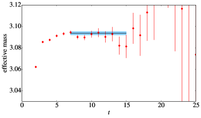
Fig. 6 shows the ratios $R_{1}$, $R_{2}$, $R_{3}$ and $R_{4}$ calculated on the $24^{3}$, $m_{l}a=0.005$ ensemble, and Fig. 7 shows the vector and pseudoscalar effective-mass plots. In all cases, we estimate the statistical error with a single-elimination jackknife. The two-point functions are fitted to a single exponential to extract $Z_{B}$ and $Z_{B^{*}}$. Using these values of $Z_{B^{(*)}}$, we then fit the ratios to a constant in the regions given in Table 4 where we expect excited-state contamination to be small. We choose the fit ranges for each ratio such that we obtain a good correlated $\chi^{2}/\mathrm{dof}$, and apply them to all ensembles of the same lattice spacing consistently.

From the ratios we use the procedure described in the previous section to extract $g_{b}$ on each ensemble, giving the values listed in Table 5.

Table 4: Fit ranges used for the two-point functions and the ratios. For non-zero momenta, equivalent combinations are averaged. Fit ranges are the same for different light-quark masses at the same lattice spacing, except in the case of the $B^{*}$ two-point function with momentum $(1,1,0)$ on $24^{3}$, $m_{l}a=0.020$ for which a range 7–15 is used in place of 9–15 listed in the table.

		fit range $t_{\mathrm{min}}$–$t_{\mathrm{max}}$
	$\vec{p}a/(2\pi/L)$	$24^{3}$	$32^{3}$
$B$	(0,0,0)	8–16	8–17
$B^{*}$	(0,0,0)	7–15	8–16
$R_{1}$	(0,0,0)	50–58	50–58
$B^{*}$	(1,0,0)	7–15	8–16
$R_{2}$	(1,0,0)	51–60	47–55
$R_{3}$	(1,0,0)	50–56	46–55
$R_{4}$	(1,0,0)	50–57	47–56
$B^{*}$	(1,1,0)	9–15	10–16
$R_{2}$	(1,1,0)	51–60	47–55
$R_{3}$	(1,1,0)	49–55	46–55
$R_{4}$	(1,1,0)	51–57	46–54

Table 5: Results for $g_{b}$ on the $24^{3}$ and $32^{3}$ ensembles. Errors for $g_{b}$ are statistical. Pion masses are from Aoki et al. (2011).

$L/a$	$m_{l}a$	$M_{\pi}^{2}/\,\mathrm{GeV}^{2}$	$g_{b}$
$24$	$0.005$	$0.108$	$0.533\pm 0.027$
$24$	$0.010$	$0.175$	$0.568\pm 0.023$
$24$	$0.020$	$0.311$	$0.580\pm 0.035$
$32$	$0.004$	$0.084$	$0.548\pm 0.020$
$32$	$0.006$	$0.119$	$0.603\pm 0.016$
$32$	$0.008$	$0.155$	$0.596\pm 0.018$

IV.2 Chiral and Continuum Extrapolations

We perform a chiral extrapolation using the SU(2) HM$\chi$PT formula for the axial coupling matrix element derived in Detmold et al. (2011):

$$g_{b}=g_{0}\left(1-\frac{2(1+2g_{0}^{2})}{(4\pi f_{\pi})^{2}}M_{\pi}^{2}\log\frac{M_{\pi}^{2}}{\mu^{2}}+\alpha M_{\pi}^{2}+\beta a^{2}\right),$$ (28)

which is next-to-leading order in the chiral expansion, but only leading order in the heavy-quark expansion. We parameterize the light-quark and gluon discretization effects with an $a^{2}$ term, as expected for the domain-wall light-quark and Iwasaki gauge actions. The lattice-spacing dependence from the RHQ action is more complicated. However, we argue in the next section that heavy-quark discretization effects are negligible and that an extrapolation in $a^{2}$ captures the leading scaling behaviour. We use the PDG value Beringer et al. (2012) of the pion decay constant, $f_{\pi}=130.4\,\mathrm{MeV}$.

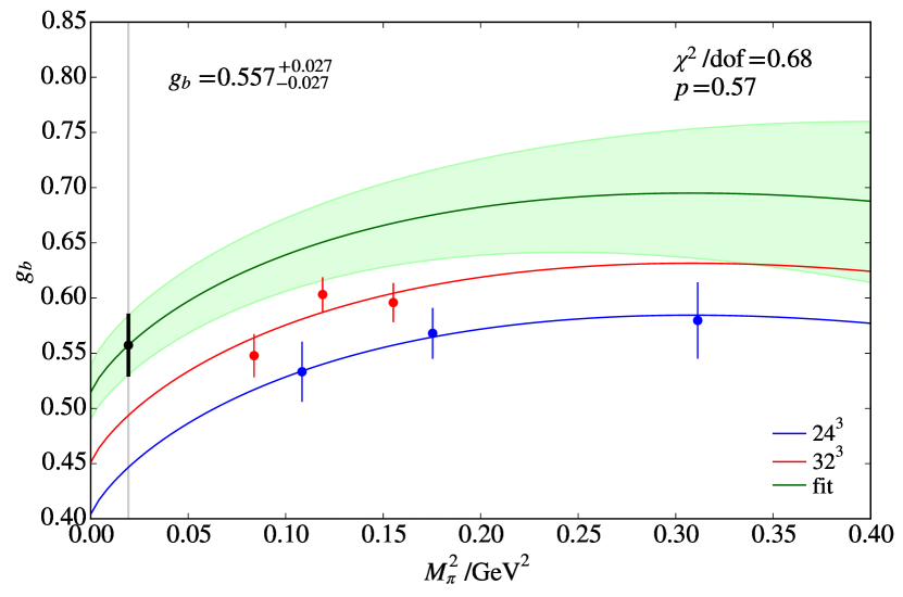
Fig. 8 shows the chiral-continuum extrapolation of the numerical simulation data to the physical light-quark mass and continuum using Eq. (28). The values of $Z_{A}$, as calculated in Allton et al. (2008) and Aoki et al. (2011), are included for each ensemble. The statistical errors in $Z_{A}$ are added in quadrature to the Monte-Carlo statistical errors in the lattice data for $g_{b}$ before performing the chiral fit. The six ensembles are statistically independent, hence the fit is calculated by minimizing an uncorrelated $\chi^{2}$ function. The parameters that minimise the $\chi^{2}$ are $g_{0}=0.515$, $\alpha=-1.324\,\mathrm{GeV}^{-2}$, $\beta=-0.648\,\mathrm{GeV}^{2}$. We use these fitted parameters and their covariance matrix to estimate the error bands in our plots and to give the errors in $g_{b}$. Our fitted result is $g_{b}=0.557\pm 0.027$.

Figure 8: Chiral and continuum extrapolation. The bottom (blue) curve is the fit through the $24^{3}$ ensemble points. The (red) curve above is the fit through the $32^{3}$ ensemble points and the (green) error band and curve show the continuum extrapolation. The intersection with the vertical grey line corresponds to the physical pion mass. The result at the physical mass is shown by the (black) point with error.

V Systematic Errors

V.1 Chiral Extrapolation

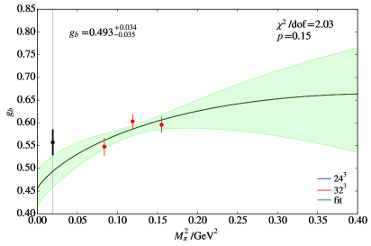
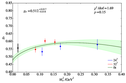
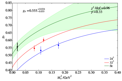
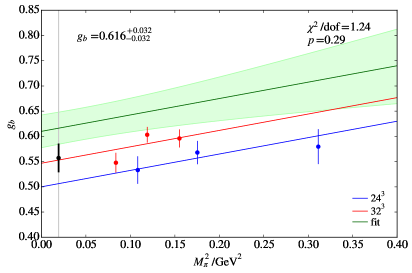
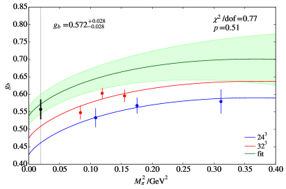
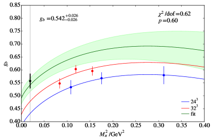
Our chiral extrapolation relies on NLO SU(2) HM$\chi$PT with pion masses above $400\,\mathrm{MeV}$. Therefore we may be using the theory beyond its range of applicability and we are certainly omitting higher order terms in the chiral expansion. To estimate the uncertainty this introduces we consider a range of possible fits. First, we consider the effect of neglecting the heaviest mass from each ensemble (center left plot in Fig. 9). This alters the form of the fit dramatically but does not significantly change the final result. In the bottom row of Fig. 9 we replace $f_{\pi}$ in the coefficient of the NLO chiral logarithms with $f_{K}=156.1\,\mathrm{MeV}$ Beringer et al. (2012) or with $f_{0}=112\,\mathrm{MeV}$ in the SU(2) chiral limit from the RBC/UKQCD light pseudoscalar meson analysis Aoki et al. (2011). This changes the relative size of NLO and NNLO and higher-order terms in the chiral expansion. Finally, we note that our data does not show any strong evidence of chiral log curvature, presumably because our lightest data point corresponds to $M_{\pi}\approx 289\,\mathrm{MeV}$ and is still rather heavy. We therefore consider an analytic fit, shown in the centre right plot of Fig. 9, where we extrapolate linearly in $M_{\pi}^{2}$. Of these variations, the largest difference from our central value for $g_{b}$ is from the linear fit in $M_{\pi}^{2}$ and $a^{2}$. This value is larger than our full chiral-continuum fit by $10.6\%$. Because the chiral and continuum extrapolations are treated together in our fitting procedure, however, discretization and chiral extrapolation errors cannot be fully disentangled. In section V.5.2 below we consider light-quark and gluon discretization errors, estimating a systematic error of $11.5\%$. This is the largest deviation seen in the chiral-continuum fits in Fig. 9 and is therefore the error we take for the combined chiral and continuum extrapolation.

Figure 9: Variations of chiral fits. Top left: $32^{2}$ data points only; top right: data points from both lattices with no $a^{2}$ term. Center left: heaviest masses dropped; center right: fit to a function linear in $M_{\pi}^{2}$. Bottom left: replacing $f_{\pi}$ with $f_{K}=156.1\,\mathrm{MeV}$; bottom right: replacing $f_{\pi}$ with $f_{0}=112\,\mathrm{MeV}$. In each plot, the result of the preferred fit from Fig. 8 is shown as the black point, with error, on the vertical line at the physical pion mass.

V.2 Lattice-scale uncertainty

The coupling $g_{b}$ is a dimensionless number calculated from ratios of correlators, so it should have only a mild dependence on the physical value of the lattice spacing. However, variations in $a$ affect the chiral and continuum extrapolations. We estimate the error in $g_{b}$ due to the lattice-spacing uncertainty by varying the $24^{3}$ and $32^{3}$ lattice spacings by their quoted (statistical plus systematic) uncertainties, $\sigma_{24}$ and $\sigma_{32}$ Aoki et al. (2011), one at a time whilst keeping the other fixed. Shifting the lattice spacing on the finest ensemble changes $g_{b}$ by $0.7\%$, and on the coarser ensemble $g_{b}$ changes by $0.6\%$. Therefore ascribing an error of $0.9\%$ (the sum in quadrature) to this source of uncertainty seems a conservative estimate.

V.3 Unphysical sea strange-quark mass

Our simulation is performed with a sea strange-quark mass that differs from the physical value by approximately $10\%$. To investigate the effect of the sea strange-quark mass on $g_{b}$ we use results from Detmold et al. (2011) for the NLO axial current matrix element in partially quenched HM$\chi$PT. This allows us to evaluate the expression with different valence and sea strange-quark masses. The NLO matrix element has four different contributions, coming from so called sunset diagrams, wave-function renormalization, tadpole diagrams and the NLO analytic terms. We have calculated the effect of a $10\%$ change in the sea strange-quark mass in the loop diagrams, assuming the values of the low-energy constants obtained from our preferred chiral fit, on the value of the coupling $g_{b}$. We find a change in $g_{b}$ of $1.5\%$. This result is numerically consistent with the effect of the strange sea-quark mass on the pion decay constant observed by the RBC/UKQCD collaboration in Aoki et al. (2011). Therefore we ascribe an error of $1.5\%$ in $g_{b}$ due to the unphysical strange-quark mass.

V.4 RHQ parameter uncertainties

V.4.1 Statistical

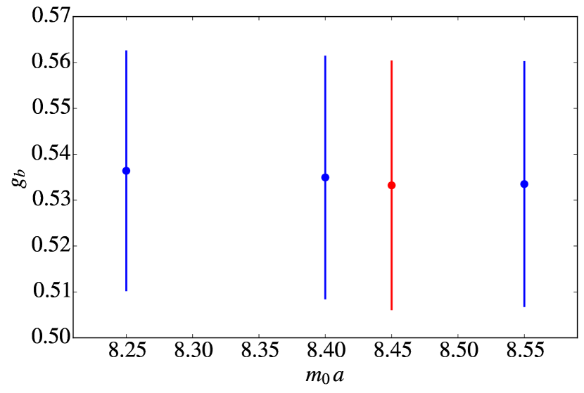
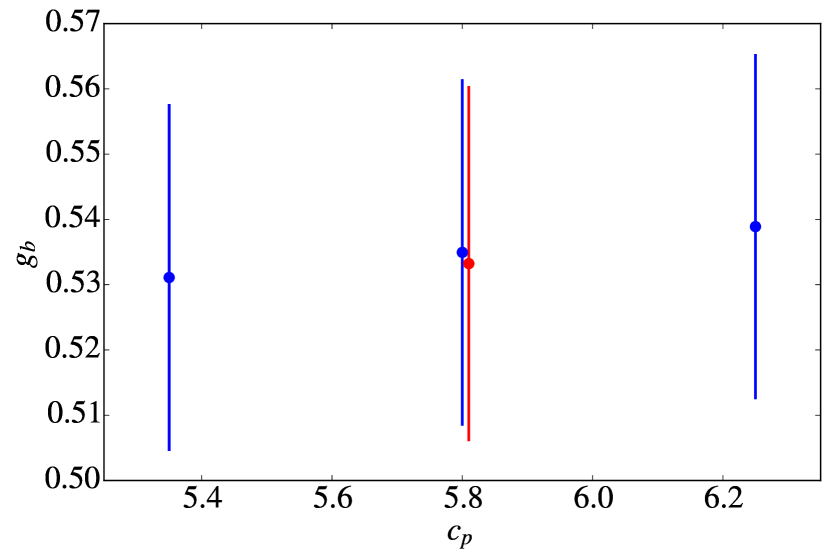
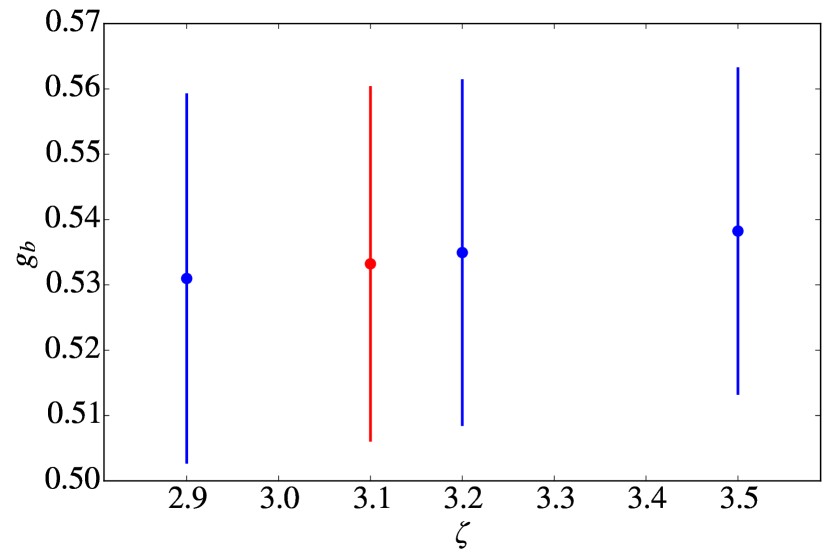
To test the dependence of $g_{b}$ on the uncertainties in the tuned RHQ parameters we calculate the coupling on the $24^{3}$ $m_{l}a=0.005$ ensemble using the full “box” of RHQ parameters used to interpolate to the tuned values:

$$\left[\begin{array}[]{c}m_{0}a\\ c_{p}\\ \zeta\end{array}\right],\left[\begin{array}[]{c}m_{0}a\pm\sigma_{m_{0}a}\\ c_{p}\\ \zeta\end{array}\right],\left[\begin{array}[]{c}m_{0}a\\ c_{p}\pm\sigma_{c_{p}}\\ \zeta\end{array}\right],\left[\begin{array}[]{c}m_{0}a\\ c_{p}\\ \zeta\pm\sigma_{\zeta}\end{array}\right].$$ (29)

For our $24^{3}$ ensembles, the box parameters are given by

$$(m_{0}a,c_{p},\zeta) =(8.40,5.80,3.20),$$ (30)

$$(\sigma_{m_{0}a},\sigma_{c_{p}},\sigma_{\zeta}) =(0.15,0.45,0.30).$$

We then linearly interpolate $g_{b}$ to the point of the tuned parameters. By following this procedure underneath the jackknife we can propagate the statistical errors from parameter tuning through to $g_{b}$. Comparison of this determination to the result calculated directly using the tuned values of the parameters gives a measure of how sensitive $g_{b}$ is to the uncertainties arising from the tuning. We find that the central values differ by $0.01\%$ and the errors agree to two significant figures. In the context of the overall uncertainty this can be considered negligible.

Figure 10 shows $g_{b}$ calculated on the seven sets of parameters indicated in Eq. (29) for the $24^{3}$ $m_{l}a=0.005$ ensemble.

Figure 10: $g_{b}$ calculated for the sets of RHQ parameters used to define the parameter “box” on the $24^{3}$ $m_{l}a=0.005$ ensemble. The blue points are the results for the box parameter choices and the red point shows $g_{b}$ calculated directly at the tuned parameter values.

V.4.2 Systematic

We also consider the effect on $g_{b}$ of systematic uncertainties in the RHQ parameters. These are estimated in Ref. Aoki et al. (2012) and given in Table 2. The three significant contributors are heavy-quark discretization effects, uncertainty in the lattice spacing, and uncertainty from the experimental inputs. To determine the sensitivity of $g_{b}$ to these uncertainties we use the calculation on the box of parameters, Eq. (29), described in the previous subsection. We assume a linear dependence of $g_{b}$ on the RHQ parameters for small shifts, then shift one parameter at a time by each systematic uncertainty and take the overall error as the effect of each of these shifts added in quadrature. The combined effect, shown in Table 6, is an error of $1.5\%$ in $g_{b}$.

Table 6: The effect of systematic uncertainties in the RHQ parameters on $g_{b}$. Each parameter was shifted by the uncertainty from each source and the effect on $g_{b}$ calculated by assuming $g_{b}$ depends linearly on the parameters.

	% error from parameter
Source	$m_{0}a$	$c_{p}$	$\zeta$	Total
HQ discretization	0.25	0.65	0.30	0.76
Lattice scale	0.97	0.65	0.24	1.19
Experimental inputs	0.14	0.33	0	0.35
Total	1.01	0.98	0.38	1.46

V.5 Discretization errors

V.5.1 Heavy-quark discretization errors

We estimate heavy-quark discretization errors using an effective field theory approach Symanzik (1983); El-Khadra et al. (1997); Oktay and Kronfeld (2008) in which both our lattice theory and QCD are described by effective continuum Lagrangians built from the same operators and errors stem from mismatches between the short-distance coefficients of higher-dimension operators in the two effective theories. Oktay and Kronfeld Oktay and Kronfeld (2008) have catalogued the relevant operators and calculated the mismatch coefficients at tree level.

Because we are evaluating a matrix element of the light-quark axial-vector current, heavy-quark discretization errors stem from mismatches in higher-dimension operators in the heavy-quark action which correct the $B$ and $B^{*}$ meson masses. We expect these effects to be negligible. From our tuning procedure Aoki et al. (2012) we can relate changes in the meson masses to changes in the RHQ parameters $m_{0}a$, $c_{p}$ and $\zeta$, while in section V.4 below, we relate changes in the RHQ parameters to changes in $g_{b}$. Hence we can estimate the effect of errors in the meson masses on $g_{b}$.

In Appendix C of Aoki et al. (2012), we estimated the heavy-quark discretization error on the spin-averaged $B_{s}$ meson mass as $0.05\%$. Also in Aoki et al. (2012), that spin-averaged mass was most sensitive to variations in $m_{0}a$, with a $0.05\%$ shift corresponding to a change of around $0.02$ in $m_{0}a$ on the $24^{3}$ $m_{l}a=0.005$ ensemble. From section V.4, shifting $m_{0}a$ by the halfwidth of our tuning “box” changes $g_{b}$ by no more than $1.5\%$. For the $24^{3}$ $m_{l}a=0.005$ ensemble, this shift in $m_{0}a$ is $0.15$ and hence we expect a heavy-quark discretization error on $g_{b}$ of no more than $(0.02/0.15)\times 1.5\%=0.2\%$, which is negligible compared to our overall uncertainty.

V.5.2 Light-quark and gluon discretization errors

Leading discretization errors from the domain-wall light-quark action and the Iwasaki gauge action are both $O(a^{2})$ and are included as an $a^{2}$ term in the combined chiral-continuum extrapolation. However the data is also compatible within errors with assuming no lattice-spacing dependence; a fit with no $a^{2}$ term also yields an acceptable, albeit larger, $\chi^{2}$/dof. The top row of Fig. 9 shows chiral fits to the data without an $a^{2}$ term. To estimate the systematic errors coming from the continuum extrapolation we use the difference of $11.5\%$ in $g_{b}$ between a fit to our finest data set ($a\approx 0.086$fm) and the $a^{2}$ extrapolation using both lattice spacings. This is the largest effect in all variations of our chiral and continuum extrapolations and is therefore the value appearing in Table 7 for the combined chiral and continuum extrapolation uncertainty.

V.6 Finite-volume effects

We expect that finite-volume effects are small since there are no propagating light particles in the simulated system. To estimate their size we compare the value of $g_{b}$ obtained from an NLO heavy-meson $\chi$PT fit to our data, with and without finite volume effects included. We compare the finite and infinite-volume fit result at all of our simulated pion-mass values. The largest finite-volume correction, which occurs for our lightest pion mass, is $\lesssim 1\%$, so we take $1\%$ as the finite-volume error in our calculation of $g_{b}$.

VI Conclusions

The sum in quadrature of all the systematic errors described in section V gives a total systematic uncertainty of 12%. Our final error budget is given in Table 7 and our final value of the coupling $g_{b}$ including statistical and systematic errors is

$$g_{b}=0.56(3)_{\mathrm{stat}}(7)_{\mathrm{sys}}$$ (31)

Table 7: Error budget for systematic and statistical errors.

Statistical errors	4.8%
Chiral and continuum extrapolation	11.5%
Lattice scale uncertainty	0.9%
Finite volume effects	1.0%
RHQ parameter uncertainties	1.5%
Unphysical sea strange-quark mass	1.5%
Systematic errors total	11.8%

Figure 11: Comparison of quenched (downward triangles), $N_{f}=2$ (upward triangles) and $N_{f}=2+1$ (circles) calculations of the couplings $g_{c}$, $g_{b}$ and $\hat{g}$ Bećirević and Sanfilippo (2013); Bećirević and Haas (2011); Abada et al. (2002, 2004); Detmold et al. (2012a); Bernardoni et al. (2015); Bulava et al. (2010); Bećirević et al. (2009); Ohki et al. (2008); Negishi et al. (2007); de Divitiis et al. (1998). Error bars represent the sum in quadrature of all quoted errors (statistical and systematic).

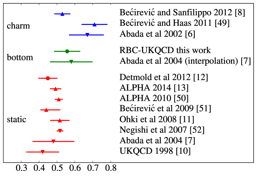
Our calculation is the first directly at the physical $b$-quark mass, and has a complete systematic error budget. Fig. 11 compares our result to earlier dynamical calculations at the charm-quark mass and in the static limit. The dependence of $g$ on the value of the heavy-quark mass is mild, and our result lies in the region that would be expected from interpolating between the charm- and infinite-mass determinations. Our result is compatible with the experimental value $g_{c}^{\mathrm{exp}}=0.570\pm 0.004\pm 0.005$ extracted from the natural linewidth of the transition $D^{*}(2010)^{+}\to D^{0}\pi^{+}$ by the BaBar Collaboration in Lees et al. (2013b). This further suggests that $1/m_{Q}^{n}$ corrections to the coupling $g$ are small. Our result has been used by the RBC/UKQCD collaboration in the chiral extrapolations of numerical lattice data for the $B$-meson leptonic decay constants Witzel (2012); Christ et al. (2015) and $B\to\pi\ell\nu$ and $B_{s}\to K\ell\nu$ semileptonic form factors Kawanai et al. (2012); Flynn et al. (2015).