Predicting the Influence of Plate Geometry on the Eddy Current Pendulum

Abstract

We quantitatively analyze a familiar classroom demonstration, Van Waltenhofen’s eddy current pendulum, to predict the damping effect for a variety of plate geometries from first principles. Results from conformal mapping, finite element simulations and a simplified model suitable for introductory classes are compared with experiments.

I Introduction

Eddy currents are induced electric currents in a conducting material that result when either the object moves through a nonuniform magnetic field or is stationary but subject to a time-changing magnetic field. They were first observed by François Arago(Babbage and Herschel, 1825) but it was not until Michael Faraday’s discovery of induction(Faraday, 1832) that the mechanism of this phenomenon was understood. A pioneering experiment to quantify the heat dissipated by the eddy currents, and hence connect electromagnetism to thermodynamics, is von Waltenhofen’s pendulum(von Waltenhofen, 1879) [figure 1(a)—(c)]. The bob of the pendulum is a non ferromagnetic conducting plate which swings between the poles of an electromagnet, generating circulating eddy currents. The dissipative eddy currents tend to oppose the motion of the bob, and hence damp the pendulum. The experiment is an example of magnetic braking: when the magnet is turned off, the pendulum oscillates as a classic pendulum, damped only by air resistance and frictional forces in the hinge; when the magnetic field is switched on, the pendulum comes to a rapid stop.

Von Waltenhofen’s pendulum is a popular demonstration in high school(Thompson and Leung, 2011) and introductory undergraduate(Onorato and Ambrosis, 2012) classes because it provides a striking visual illustration of the invisible eddy currents. It is easy to set up, and gives the instructor a chance to discuss real-world applications such as magnetic braking in roller coasters, hybrid cars and the detection of flaws in conductive materials. Moreover, by using different shaped plates as bobs, some of the characteristics of eddy currents can be explored: if the plate is now substituted with one where the slits do not reach the edges [figure 1(d)(ii)], the damping is only mildly altered. If a solid plate is replaced by a comb-like plate with slits cut into it [figure 1(d)(iii)-(iv)] the damping effect is greatly attenuated. Students infer from this that the eddy currents must be localized to some region of the plate.

Typically, however, the relationship between the shape of the plate and the damping is considered only qualitatively due to the complexity of the calculations required, which require advanced mathematical techniques introduced in higher-level electromagnetism classes. In this paper, therefore, we apply some of these strategies to predict the damping behavior of conducting plates with different geometries. We investigate four plate shapes, illustrated in figure 1(d): (i) a square plate, (ii) a plate with holes that do not reach the edge, (iii) a plate with with two slots, (iv) another with four slots. The present work was primarily performed during a project-based graduate electrodynamics class with the objective of giving students a real, tractable example of the utility of their calculations. It was also an opportunity to address the challenges of connecting theory to experiment, even where the fundamental theory is uncontroversial.

The paper is organized as follows: in section II, the form of the damping for the present experiment is derived first in terms of a simplified model suitable for undergraduate classes and the effect of these damping terms on the simple pendulum is explored. In section III, we present a more sophisticated model derived from Maxwell’s equations in the magneto-quasistatic approximation. Within this framework, the rate of power dissipation for each plate is estimated using a conformal mapping technique and a finite element solution. In section IV, the motion of the pendulum with each of the four plates is determined experimentally and compared with the predictions of each of the theoretical models in section V. In section VI, the pedagogical context of this work is discussed. Brief conclusions are presented in section VII.

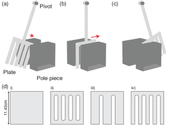
Figure 1: Schematic of Von Waltenhofen’s pendulum. (a) An aluminium plate swings between the pole pieces of an electromagnet. As it passes through the fringing field, eddy currents are induced in the plate that dissipate energy and damp the pendulum. (b) As the plate passes through the center of the pole pieces, the rate of change in flux through the plate vanishes and so the eddy current momentarily vanishes. (c) As the pendulum swings back, the eddy current reverses direction. (d) Various plate geometries under investigation in the present work (to scale).

II Simplified Model

The damped simple pendulum is, in the presence of dissipative forces, described by the equation,

$$\ddot{q}+\omega_{0}^{2}q+\frac{\partial D}{\partial\dot{q}}=0$$ (1)

where $D(q,\dot{q})$ is the Rayleigh dissipation function, $\omega_{0}$ is the natural frequency of the pendulum and $q(t)$ is a generalized coordinate. In the absence of the magnetic field, a Stokes-like drag is assumed,

$$D_{stokes}=\beta\dot{q}^{2},$$ (2)

arising from friction in the bearing and air resistance. In this section and the next, the form of the dissipation function in the presence of the magnetic field is derived, first for a simplified model suitable for introductory classes and second a more physically correct model based on the magneto-quasistatic approximation. The remaining theory section considers the effect of these terms on the solutions of (1).

To develop the simplified model, we make the gross approximation that the eddy currents are completely localized to the boundary of the plate. Then, the plate may be replaced by a thin closed loop of wire of equivalent shape with area $A$, length $L$, resistivity $\rho$ and with a normal unit vector $\hat{\mathbf{n}}$. The magnetic flux passing through the loop is,

$$\Phi=\int\mathbf{B}\cdot d\mathbf{A}=\left\langle\mathbf{B}\right\rangle A$$ (3)

where $\left\langle\mathbf{B}\right\rangle$ is the mean value of the magnetic field over the plate when it is located at a particular position $q$. The emf induced around the loop is, by the Faraday-Lenz law and using the chain rule,

$$V=-\frac{\partial\Phi}{\partial t}=-\frac{\partial\Phi}{\partial x}\dot{q}=-A\frac{d\left\langle\mathbf{B}\cdot\hat{\mathbf{n}}\right\rangle}{dq}\dot{q}.$$ (4)

The power dissipated in the loop is precisely the dissipation function desired and readily calculated,

$$D=V^{2}/R,$$ (5)

which, using $R=\rho L$, becomes,

$$D=\underbrace{\left(\frac{A^{2}}{L}\right)}\frac{1}{\rho}\left(\frac{d\left\langle\mathbf{B}\cdot\hat{\mathbf{n}}\right\rangle}{dq}\right)^{2}\dot{q}^{2}$$ (6)

where the highlighted term represents the “geometric factor” arising from the shape of the plate. The dissipation function (6) has the form of a position-dependent Stokes drag.

It is now necessary to solve the pendulum equation including the new dissipation terms (6),

$$\ddot{q}+\omega_{0}^{2}q+2\left[\beta+\frac{A^{2}}{L\rho}\left(\frac{d\left\langle\mathbf{B}\cdot\hat{\mathbf{n}}\right\rangle}{dq}\right)^{2}\right]\dot{q}=0,$$ (7)

for which the form of the magnetic field must be known. Here, the coordinate system is oriented as shown in figure 1 such that the plate normal $\hat{\mathbf{n}}$ is parallel to the $z$ axis, so only $B_{z}$ is required; the origin is chosen to lie in the middle of the pole pieces. An approximation made in other studies(Thompson and Leung, 2011; Onorato and Ambrosis, 2012) is that the magnetic field is constant between the pole pieces and zero everywhere else, i.e. that,

$$B_{z}=\begin{cases}B_{0}&-L_{pp}/2\leq x<L_{pp}/2\\ 0&x<-L_{pp}/2,\ x\geq L_{pp}/2\end{cases}$$ (8)

where $L_{pp}$ is the width of the pole pieces. If the plate is square of side $L$, the average value of the field over the surface of the plate when it is centered at $q$ along the $x$-axis may be determined,

$$\left\langle\mathbf{B}\cdot\hat{\mathbf{n}}\right\rangle=L\int_{q-L/2}^{q+L/2}B_{z}(x^{\prime})\ dx^{\prime}.$$ (9)

For the ansatz (8), the flux through the plate increases (decreases) linearly as it enters (leaves) the field. Depending on the size of the plate, and the amplitude of the motion, the plate may also experience portions of the motion where there is no change in flux. If the plate is the same size as the pole pieces $L=L_{pp}$, and never fully leaves the field, i.e. $\left|x\right|<(L_{pp}+L)/2$ , then $\left\langle\mathbf{B}\cdot\hat{\mathbf{n}}\right\rangle\sim B_{0}q$ and the classical damped pendulum is recovered, but with a modified damping constant,

$$\ddot{x}+\omega_{0}^{2}x+2\left[\beta+\frac{A^{2}B_{0}^{2}}{L\rho}\right]\dot{x}=0.$$ (10)

In order to gauge the validity of the (8) for the pendulum we calculated the spatial dependence of the magnetic field due to the pole pieces in the magnetostatic formulation, using a scalar potential function defined $\mathbf{B}=-\nabla\phi$ and subject to Laplace’s equation $\nabla^{2}\phi=0$. This was solved using the finite element software FlexPDE for square pole pieces of width $11$cm and separation $3.5$cm. Dirichlet boundary conditions were imposed on the pole pieces. A plot of $B_{z}$ along the horizontal centerline of the midplane of the pole pieces is displayed in fig. 2(a), showing as expected that the field is constant between the pole pieces with the fringing field decaying rapidly outside. From this calculated profile, the flux $\int\mathbf{B}\cdot d\mathbf{A}$ through a square plate placed at different horizontal positions was also calculated; the result is displayed in fig. 2(b). Notice that the flux depends linearly on position for $1\lesssim\left|x\right|\lesssim 10$cm, suggesting that the equation of motion (10) is likely to be valid for moderate amplitudes; however around $x=0$ the flux depends quadratically on $x$, suggesting that (10) is likely to be inaccurate for small amplitudes.

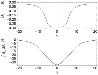
Figure 2: (a) Field strength as a function of distance $x$ through the center of the pole pieces. (b) Magnetic flux through a square plate as a function of the position of the plate $x$.

III Magneto-quasistatic Model

Since the eddy current is not strictly confined to the edges of the plate, it is necessary to develop a more sophisticated model by solving Maxwell’s equations

$$\nabla\cdot\mathbf{E}=0,\ \nabla\cdot\mathbf{B}=0,\ \nabla\times\mathbf{H}=\mathbf{J},\ \nabla\times\mathbf{E}+\frac{\partial\mathbf{B}}{\partial t}=0$$ (11)

together with the continuity equation

$$\nabla\cdot\mathbf{J}+\frac{\partial\rho}{\partial t}=0$$ (12)

to determine the true current density in the plate. Here, the magneto-quasistatic approximation(Jackson, 1975) has been made, i.e. the Maxwell correction to Ampere’s law is neglected. This is justified because the timescale of variation of the magnetic field over the surface of the plate is sufficiently long that the eddy current produced does not significantly alter the magnetic field in turn.

To perform the analysis, consider a thin metal plate of uniform conductivity $\sigma$ and thickness $d$ and where the shape of the plate is arbitrary. It is assumed that Ohm’s law holds for the plate, so

$$\mathbf{J}=\sigma\mathbf{E}.$$ (13)

In the frame of the laboratory, since the pendulum is rigid, the position of the plate may be described by the single generalized coordinate $q(t)$ in eq. 1. As the pendulum swings, the plate passes through regions of different magnetic field strength. Viewed from the point of view of the plate, the magnetic field across its surface changes as a function of time. This may be described by defining a local coordinate system $(x^{\prime},y^{\prime},z^{\prime})$ relative to the plate such that the plate lies in the $x^{\prime}-y^{\prime}$ plane, and considering the magnetic field in this frame,

$$\mathbf{B}=\mathbf{B}(x^{\prime},y^{\prime},q(t)).$$ (14)

We note that the reference frame $(x^{\prime},y^{\prime},z^{\prime})$ is not an inertial frame as the pendulum undergoes periodic acceleration during the course of its motion; however we neglect these effects as the pendulum velocity $r\dot{q}\ll c$. By Faraday’s law, an electric field and hence an eddy current is induced in the plate: if $d\ll\delta$ the skin depth of the material it may be assumed that $\mathbf{E}$ is oriented in the $x-y$ plane and does not vary significantly over the thickness of the plate; hence the problem is quasi-two-dimensional.

From equations (11) and (13), it is a standard textbook problem to show that the quantities $\mathbf{E}$, $\mathbf{B}$, $\mathbf{A}$ and $\mathbf{J}$ all obey the diffusion equation,

$$\nabla^{2}\mathbf{J}=\sigma\frac{\partial\mathbf{J}}{\partial t}.$$ (15)

Since $\rho=0$, the continuity equation implies that $\mathbf{J}$ must have no divergence and hence can be written using a stream function,

$$J_{x}=\frac{\partial\phi(x^{\prime},y^{\prime})}{\partial y},\ J_{y}=-\frac{\partial\phi(x^{\prime},y^{\prime})}{\partial x^{\prime}}.$$ (16)

By inserting (16) into (15), together with the given applied Magnetic field into Maxwell’s equations, it may be shown that the stream function obeys Poisson’s equation

$$\nabla^{2}\phi(x^{\prime},y^{\prime})=\sigma\frac{d\mathbf{B}\cdot\hat{\mathbf{n}}}{dq}\dot{q}=B_{0}\sigma\dot{q}\zeta(\mathbf{x}^{\prime},q)$$ (17)

where $\nabla$ here is the 2D Laplacian, $B_{0}$ is the magnetic field strength and we defined a source term $\zeta(\mathbf{x},q)=\frac{d\mathbf{B}\cdot\hat{\mathbf{n}}}{dq}/B_{0}$. Since $\mathbf{J}$ must lie tangentially to the edge of the plate, $\phi$ obeys a Dirichlet boundary condition $\phi=0$ on all edges of the plate. From the solution for $\phi$, the instantaneous rate of power dissipation by the plate is then calculated,

$$D=\frac{d}{\sigma}\int\left|\mathbf{J}\right|^{2}\ \text{d}A,$$ (18)

where the integral is to be taken over the plate. Inserting the stream function (16) into (18), integrating by parts and using (17), we obtain

$$D = \frac{d}{\sigma}\int\nabla\phi\cdot\nabla\phi\ \text{d}A,$$ (19)

$$= \frac{d}{\sigma}\left(\oint\phi\nabla\phi dl-\int\phi\nabla^{2}\phi\ dA\right)$$ (20)

$$= -d\dot{q}B_{0}\int\phi\zeta(\mathbf{x}^{\prime},q)\ dA.$$ (21)

A formal solution to (17) may be constructed using the Green function for the Laplacian,

$$\phi(\mathbf{x}^{\prime})=\sigma\dot{q}B_{0}G\zeta=\sigma\dot{q}B_{0}\int G(\mathbf{x}^{\prime},\mathbf{x}^{\prime\prime})\zeta(\mathbf{x}^{\prime\prime},q)\ dA^{\prime\prime}.$$ (22)

Inserting this into (21) and rearranging we obtain the dissipation function,

$$D(q,\dot{q}) = -dB_{0}\dot{q}\int\left[\sigma B_{0}\dot{q}\int G(\mathbf{x}^{\prime},\mathbf{x}^{\prime\prime})\zeta(\mathbf{x}^{\prime\prime},q)\ dA^{\prime\prime}\right]\zeta(\mathbf{x}^{\prime})\ dA^{\prime}$$ (23)

$$= -d\sigma B_{0}^{2}\dot{q}^{2}\int\int\zeta(\mathbf{x}^{\prime},q)\zeta(\mathbf{x}^{\prime\prime},q)G(\mathbf{x}^{\prime},\mathbf{x}^{\prime\prime})\ dA^{\prime}\ dA^{\prime\prime}.$$ (24)

Since the source function $\zeta(\mathbf{x},q)$ depends on the position of the pendulum $q$, this has the form

$$D(q,\dot{q})\propto B_{0}^{2}P(q)\dot{q}^{2}$$ (25)

where we define a local dissipation rate $P(q)$. To determine an effective damping coefficient, the calculations proceed as follows: in subsection III.1 the form of $\zeta(\mathbf{x},q)$ is determined, then the positional dependence of the drag term is evaluated using a conformal mapping technique in subsection III.2, and also by solving (17) with FlexPDE in subsection III.3; finally, the effect of the position dependent damping on the motion of the pendulum is considered in the subsection III.4.

III.1 Evaluating the Fringe field

Before evaluating the power dissipation, it is first necessary to determine the functional form of the magnetic fringe field that the plate experiences as it moves between the pole pieces and hence the function $\zeta(x)$. This could also be obtained from a finite element calculation as was done for the simplified model in section (II). We made the approximation that only the fringe fields from the sides of the pole pieces are significant in the damping, and the vertical extent of the pole pieces are neglected; the formulation above remains sufficiently general that these details could easily be included in a more sophisticated calculation of $\zeta(x)$.

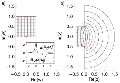
Figure 3: Conformal mapping $z(w)$ from (a) a portion of the strip $0\leq\Im(w)\leq 1$ to (b) the depicted region in the $z$ plane. Places where the integrand in (26) vanishes are indicated by red circles; these introduce corners into the map. Contours of constant $\Re(w)$ (dashed lines) and $\Im(w)$ (solid lines) and their projection are indicated corresponding to equipotentials and field lines respectively. Inset: Plots of the field profile $B_{z}(x)$ and its spatial derivative $B_{z}^{\prime}(x)$ calculated from the conformal mapping.

Within this approximation, the problem is two dimensional and hence can be solved using conformal mapping, an important technique for solving electrostatics problems. For a full discussion we refer the reader to (Needham, 1999) and (Driscoll and Trefethen, 2002). Briefly, however: A map from a domain to its image is called conformal if angles measured locally around a point in the source domain are preserved under the mapping. A key property of such maps is that if a function that is a solution to Laplace’s equation is constructed on some domain, then the projection of that function under the action of the mapping will also obey Laplace’s equation. Boundary value electrostatics problems in two dimensions can hence often be solved using this method by constructing a solution to Laplace’s equation with appropriate boundary conditions in some simple domain and then finding a conformal map to the domain of interest. The powerful Riemann mapping theorem guarantees such a map exists if the domains are simply connected; mappings between multiply-connected domains may also exist if certain compatibility criteria are met(Driscoll and Trefethen, 2002). A rich source of such maps are analytic complex functions $z(w)$ that map a domain in the complex plane $w=u+iv$ to an image in the plane $z=x(u,v)+iy(u,v)$. The required mapping to find the fringe field is,

$$z(w)=\int_{0}^{w}\exp(-\pi\xi/2)\left[\sinh\left(\pi\xi\right)\right]^{1/2}\ d\xi.$$ (26)

As shown in figure 3, this maps the strip defined by $0\leq\Im(w)\leq 1$ in the $w=u+iv$ plane onto the depicted region in the $z=x+iy$ plane; the resulting shape resembles an overhead view of the edge of two parallel pole pieces. The integrand in (26) vanishes at $\xi=0$ and $\xi=\imath$. The effect of these poles is to introduce corners in the map; the angle of these is controlled by the strength of the pole, here $1/2$. The factor of $\exp(-\pi\xi/2$) is required to ensure that the boundary of the $\Re(w)<0$ part of the strip remains horizontal while the $\Re(w)>0$ half is mapped to the vertical boundaries. The integral can be performed analytically,

$$z(w)=\frac{\sqrt{2}}{\pi}e^{-\frac{\pi w}{2}}\left(1+\frac{e^{\pi w}\arcsin\left(e^{\pi w}\right)}{\sqrt{1-e^{2\pi w}}}\right)\sqrt{\sinh(\pi w)},$$ (27)

where the overall prefactor is chosen to ensure that the $\Re(w)<0$ half of the strip is mapped onto $0\leq\Im(z)\leq 1$.

The magnetic field strength can be determined using this map as follows: in the space between the pole pieces $\nabla\cdot\mathbf{B}=0$ and hence the magnetic field can be constructed from a scalar potential $\mathbf{B}=-\nabla\psi$ subject to Laplace’s equation $\nabla^{2}\psi=0$. On the boundary, $\mathbf{B}$ must be perpendicular to the pole pieces so these must be surfaces of constant $\psi$. In the $w$-plane, the system resembles a parallel plate capacitor with the solution $\psi=Av+B$ where $A$ and $B$ are arbitrary constants. Since Laplace’s equation is invariant under the conformal mapping, this solution remains valid when projected into the $z$-plane: the lines of constant $v$ are equipotentials and lines of constant $u$ are the field lines as shown in figure 3.

The magnetic field can be found from $\mathbf{B}=-A\left(\partial_{x}v,\partial_{y}v\right)$ ; this can be expressed in complex form in the $w$-plane as $B(w)=-A/z^{\prime}(w)$(Needham, 1999). Evaluating $z(w)$ and $B(w)$ along the center of the strip $w=t+i/2$ yields $B_{y}^{0}$ along the midplane; the $x$ derivative of $B_{y}$ required for the pendulum motion is evaluated from these using the chain rule,

$$x = \frac{1}{\pi}\left[e^{\pi t}\sqrt{1+e^{-2\pi t}}-2\text{arccosh}(e^{\pi t})\right]$$

$$B_{y}^{0} = \left(1+e^{2\pi t}\right)^{-1/2}$$

$$\frac{\partial B_{y}^{0}}{\partial x} = -\frac{1}{4}\pi\text{sech}(\pi t)^{2}.$$ (28)

Having tabulated values of $B_{y}^{\prime}(x)$ using the above implicit expressions, a final form for $\zeta(x)$ was assembled from two appropriately translated and rescaled copies of $B_{y}^{\prime}(x)$ as shown in the inset of figure 3; this was used in subsequent calculations as an InterpolatingFunction in Mathematica, or exported as a table for use in FlexPDE. For the plates and pole pieces considered, it is actually the case that the plates were slightly larger than the width of the pole pieces; while this could easily be accommodated by a simple rescaling of the solution (28), it was found in practice not to affect the dissipation enough to affect the quality of the fit.

III.2 Conformal Mapping Solution

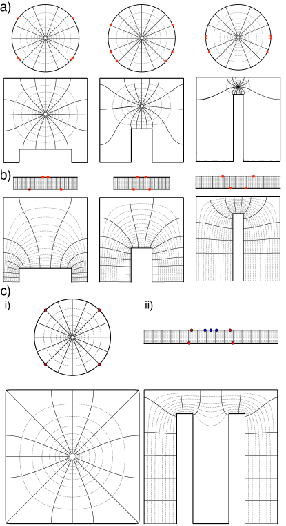
Figure 4: (a) Map from the unit circle to a paddle with a single slit of variable geometry. (b) Map from a rectangular domain to the slit. The position of poles in the canonical domains is indicated with red circles; these become vertices in the image domain. (c) Two maps relevant to the experiment: i) map from a circle to a square; ii) map from a rectangular domain to a square with two slits—note significant crowding in the central spar.

Conformal mapping can be also used to evaluate the power dissipation of the plate as it passes through the fringing field. The strategy here is to find a mapping from a simple canonical domain on which the Green function is known to one that approximates the shape of the plates; then the integral (24) can be computed. As will be seen, the choice of canonical domain is important to render the problem tractable. We therefore examined two choices: first, the mapping from the unit circle ($w$-plane) to a polygon of interest ($z$-plane) defined by an ordered set of vertices $z_{i}^{0}$ is given by the Schwarz-Christoffel formula(Driscoll and Trefethen, 2002),

$$z=A+C\int^{w}\prod_{i}(\xi-w_{i}^{0})^{-\alpha_{i}}\ d\xi$$ (29)

where $\alpha_{i}$ is the exterior turning angle of the polygon at vertex $i$ and the $w_{i}^{0}$ are the points on the unit circle that are mapped to the vertices of the polygon $z_{i}^{0}$. The constants $A$ and $C$ are translation and scaling factors respectively. While the set of parameters $\{\alpha_{i}\}$ can be determined directly from the polygon, the positions of the parameters $\{w_{i}^{0}\}$ must be determined numerically(Driscoll and Trefethen, 2002). $A$ and $C$ are then determined to rotate and scale the result onto the polygon of interest. Some representative results for a single slit are shown in fig. 4(a). Due to the symmetry of the problem, the position of three poles must be determined numerically with the remaining vertices provided by reflection.

The second choice of canonical domain is a rectangular portion of the semi-infinite strip, $-W<\Re(w)<W$ , $0<\Im(w)<1$. A mapping onto the shape of interest is given by,

$$z=A+C\int^{w}\prod_{i}\left(\sinh\left[\frac{\pi}{2}\left(w-w_{i}^{0}\right)\right]\right)^{-\alpha_{i}}\ d\xi$$ (30)

where similarly $w_{i}^{0}$ are the position of the poles which produce the required corners in the image domain and $\alpha_{i}$ are the turning angles; this formula is a more general version of equation (26) used to determine the fringing field. Results for the single slit are shown in fig. 4(b). Note that this map is approximate only: the left and right sides of the rectangle are mapped to the bottom of the paddle—the side that the slit is on—but their image under (30) is not a straight line. Hence, only two poles $\{w_{i}^{0}\}$—mapped to the interior vertices of the slit—need be determined numerically; the third parameter is the width of the rectangle $W$. Despite the approximate nature of the map, the distortion of the lower boundary is very small. These parameters were found by minimizing an objective function that was constructed from the $L_{2}$ norm of the difference between the ratios of the sides of the polygon and their desired values; a notebook to do so is provided as Supplementary Material. Robust numerical codes including SCPACK(Trefethen, 1980) and the SC Toolbox(Driscoll, 1996) are available for more complex shapes.

Comparing the two choices of canonical domain in figure 4, an important difference is apparent. The poles in the maps from the unit circle tend to lie very close to one another, becoming in some cases indistinguishable in the figure, though they remain numerically distinct. As a consequence of this phenomenon, known as crowding(Driscoll and Trefethen, 2002), very small regions adjacent to these crowded poles are mapped to large regions in the image domain. Crowding is problematic, because it makes numerically finding the $w_{i}^{0}$ challenging; it will also cause problems in evaluating the power dissipation. Notice that using the rectangular source domain eliminates the crowding problem as the poles remain well-separated.

In fig. 4(c), we show two maps relevant to the experiment. First, the map from the circle to the square is famously

$$z=A+C\int^{w}\frac{1}{\sqrt{1+\xi^{4}}}\ d\xi.$$ (31)

An example with two slits that closely matches the experimental plate is shown in fig. 4(c)(ii), constructed by introducing additional poles into one side of the one-slit rectangle maps above. Unfortunately, the crowding phenomenon is visible in this map: a very small piece of the rectangle is mapped to the central spar of the plate. As will be seen later, this will reduce the accuracy of the power dissipation calculation when this spar coincides with the edge of the pole pieces. While it is possible to find maps with crowding localized to different portions of the plate(Driscoll and Trefethen, 2002), it cannot be alleviated entirely if more than one slit is present. Hence, we did not pursue maps for plates with more than 2 slits.

Turning, then, to the issue of evaluating the power dissipated by the induced current, we initially tried to use the eigenfunction expansion of the Green function,

$$G(\mathbf{x}^{\prime},\mathbf{x}^{\prime\prime})=\sum_{n}\frac{\psi_{n}(\mathbf{x})\psi_{n}(\mathbf{x}^{\prime})}{\lambda_{n}},$$ (32)

which, inserted into the integral in (24) allows one to obtain,

$$\int\int\zeta(\mathbf{x}^{\prime},q)\zeta(\mathbf{x}^{\prime\prime},q)G(\mathbf{x}^{\prime},\mathbf{x}^{\prime\prime})\ dA^{\prime}\ dA^{\prime\prime}$$ (33)

$$=\sum_{n}\frac{\left[\int\zeta(\mathbf{x},q)\psi_{n}(\mathbf{x})\ dA\right]^{2}}{\lambda_{n}}$$ (34)

The 2D integral in (33) can then be performed in the $w$-plane using the normalized eigenfunctions of the unit disk and the mapping $z(w)$,

$$\int\zeta(\mathbf{x})\psi_{n}(\mathbf{x})\ dA=\int\zeta(z(w),q)\psi_{n}(w)\left|z^{\prime}(w)\right|^{2}\ dw.$$ (35)

Unfortunately, we found that the series (34) converges very slowly except for the square map (31). The problem is further compounded for the unit circle by the fact that the integrand in (35) is very sharply peaked and localized to the boundary in many cases due to crowding. For these reasons, we abandoned this approach and the unit circle maps as viable means to evaluate the dissipation.

The power dissipation integral (24) can be re-expressed in the $w$-plane as,

$$D\propto\int\int\zeta(z(w^{\prime}),q)\zeta(z(w^{\prime\prime}),q)G(w^{\prime},w^{\prime\prime})\left|z^{\prime}(w^{\prime})\right|^{2}\left|z^{\prime}(w^{\prime\prime})\right|^{2}\ dw^{\prime}\ dw^{\prime\prime}.$$ (36)

In order to evaluate this integral, one requires a numerically efficient representation of the Green function. Unfortunately, the Green’s function for a rectangle cannot be expressed in closed form, requiring expensive evaluation of elliptic integrals. Recently, however, renewed interest in Green function methods has yielded rapidly converging series representations(Melnikov and Melnikov, 2006). Briefly, the strategy is to start from the eigenfunction expansion of $G(w,w^{\prime})$ (32) on the rectangle and separate the double summation into two pieces: one that can be summed analytically and a second that remains to be performed numerically. Fortuitously, the analytical part contains the inherent singularity; the remaining numerical sum is a smooth function requiring few terms to converge to machine precision. Equation (7) of (Melnikov and Melnikov, 2006) presents an expression for the green function in a square; we derived an equivalent expression for the rectangle $-W<\Re(w)<W$ , $0<\Im(w)<1$ of interest,

$$G(w,w^{\prime})=\frac{1}{2\pi}\ln\frac{\left|1-e^{w-\bar{w^{\prime}}}\right|\left|1-e^{w+\bar{w^{\prime}}}\right|}{\left|1-e^{w-w^{\prime}}\right|\left|1-e^{w+w^{\prime}}\right|}-\frac{2}{\pi}\sum_{n=1}^{\infty}\frac{\sinh\left(n\pi u\right)\sinh\left(n\pi u^{\prime}\right)}{ne^{2n\pi W}\sinh\left(2n\pi W\right)}\sin\left(n\pi v\right)\sin\left(n\pi v^{\prime}\right)$$ (37)

where $w=u+iv$ and $w^{\prime}=u^{\prime}+iv^{\prime}$ consistent with our earlier definitions.

Inserting (37), (30) and $\zeta(x)$ derived in the previous section into (36), we evaluated the local power dissipation rate $P(q)$ as a function of $q$ for a variety of plate geometries. A notebook to perform these calculations is presented as Supplementary Material; we defer consideration of the results until the subsequent section, in which the same function is calculated by finite element simulations.

III.3 Finite Element Simulations

Figure 5: (a) Dissipation rate as a function of position and (b) i-iv corresponding current density profiles obtained numerically for the various shapes from FlexPDE.

Finite element analysis is a commonly used numerical technique for solving partial differential equations in systems too complicated for analytical solution. Here, the PDE of interest is, as shown in the previous sections, Poisson’s equation with a spatially dependent source term (17). This must be solved to obtain the stream function $\phi(x^{\prime},y^{\prime})$ for each of the paddle shapes of interest and at each point $q$ in the motion of the paddle. Suitable input files for FlexPDE for each plate are included as Supplementary Material. Each script contains field variable and parameter definitions, a definition of the PDE, a description of the appropriate domain boundary and specification of the boundary conditions, and a list of the outputs desired, i.e. $\phi$, $\mathbf{J}$ and the value of the integral (24). A relative error of $<10^{-4}$ in the absolute $\phi$ was requested and used by FlexPDE to guide adaptive refinement.

For each plate, the boundary condition on the exterior is simply $\phi=0$, which forces the stream function to lie tangentially to the edge of the plate. The plate with holes requires special treatment: around each of the holes $\phi$ should be constant, i.e. the hole should be an equipotential surface, but the correct value is not a priori known. A way to obtain the correct solution is to exploit an electrostatic analogy, modifying Poisson’s equation by introducing a permittivity $\epsilon$,

$$\nabla\cdot(\epsilon\nabla\phi)=\zeta(x^{\prime},q).$$ (38)

The computational domain is extended so that $\phi$ is also defined inside the holes. Different values of $\epsilon$ are used for the interior of the plate $\epsilon_{plate}$ and the holes $\epsilon_{holes}$. As the ratio $\epsilon_{holes}/\epsilon_{plate}\to\infty$, the solution converges to the desired solution where $\phi$ constant inside the holes. For the purposes of calculation, $\epsilon_{plate}$ is chosen arbitrarily to be $1$ and $\epsilon_{holes}$ is successively increased; the value of (24) converged to a relative error of $10^{-3}$ for $\epsilon_{holes}>10^{4}$. Plots of the stream function $\phi$ and the corresponding current densities $\mathbf{J}$ resulting from the calculations are displayed in figure 5, together with a plot of the dissipation rate $P(q)$.

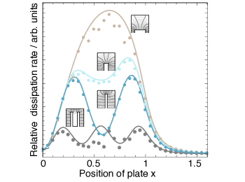
Figure 6: Comparison of finite element (solid lines) and conformal mapping (points) approaches to calculating the local rate of dissipation $P(q)$.

It is now possible to compare the Conformal Mapping and Finite Element methods for this problem. To do so, we used both methods to calculate the dissipation rate $P(q)$ for the plate geometries displayed in fig. 4(b) and (c), i.e. those for which we were able to find appropropriate mappings. To perform the integral (36), we used Mathematica’s NIntegrate with the AdaptiveMonteCarlo method and $10^{5}$ evaluation points. The calculation for each plate took $\sim 5$ minutes for FlexPDE and $\sim 20$ minutes for the conformal mapping approach on the same computer (Apple Macbook Air 11” Late 2014). Results for the various plates are shown in fig. (6). The agreement is very good for the single slit geometries, with the position and size of extrema reproduced well by both methods. For the two slit geometry, however, the conformal mapping method performs less well: the outer maxima are reproduced well, but the central one is not. This corresponds to the positioning of the plate where the edge of the pole piece coincides the central spar, where as discussed in section III.2 the mapping is crowded. Clearly from this comparison, the method of choice appears to be finite elements, since the results are less noisy and all plate shapes can be simulated using the method.

III.4 Effect on the Motion of the Pendulum

Having formulated both models, we turn to the effect of the dissipation on the motion of the pendulum. For both the simplified wire model of section II and the magneto-quasistatic model of section III, the equation of motion has the form,

$$\ddot{x}+\omega_{0}^{2}x+\lambda(x)\dot{x}=0.$$ (39)

For the wire model,

$$\lambda_{wire}=2\left[\beta+\left(\frac{A^{2}}{L}\right)\frac{B_{0}^{2}}{\rho}\right]$$ (40)

as read off from eq. (10); for the magneto-quasistatic model the Stokes drag is supplemented by the position-dependent dissipation rate,

$$\lambda_{mqs}=2\beta+d\sigma P(q)B_{0}^{2}.$$ (41)

As is well-known, the equation of motion (39) with constant $\lambda$ can be solved analytically yielding,

$$x(t)=x_{0}e^{-\lambda t/2}\cos(\omega^{\prime}t+\phi)+x_{1}$$ (42)

where $x_{0}$ and $x_{1}$ are amplitude and offset parameters, $\phi$ is a phase and $\omega^{\prime}=\sqrt{\omega^{2}-\lambda^{2}}$. Hence, the motion remains oscillatory for $\omega>\lambda$. If the plate is centered with respect to the pole pieces, $x_{1}=0$; $q_{0}$ and $\phi$ similarly represent initial conditions that are experimentally controllable. Rather than fit to the entire trajectory, it is convenient to look only at the extreme points where the pendulum is stationary and $\cos(\omega_{0}t+\phi)=\pm 1$. Inserting this into (42) and rearranging, we obtain

$$\log|x(t)|=\log x_{0}-\lambda t/2,$$ (43)

showing that the values of the position of the pendulum at successive stationary points should obey a linear relation on a plot of $\log(x)$ versus $t$.

For the magneto-quasistatic model, analytical solution of (39) is impossible and hence the equation must be solved numerically. This was performed in Mathematica. Because the strategy of looking at successive extrema on log scales remains a valuable fitting strategy even if the equation of motion is solved numerically, we additionally incorporated an extremum-finding routine to identify the stationary points from the calculated trajectory. With these simplified analytical and numerical magneto-quasistatic models, we are now ready to compare them with experimental data.

IV Experiment

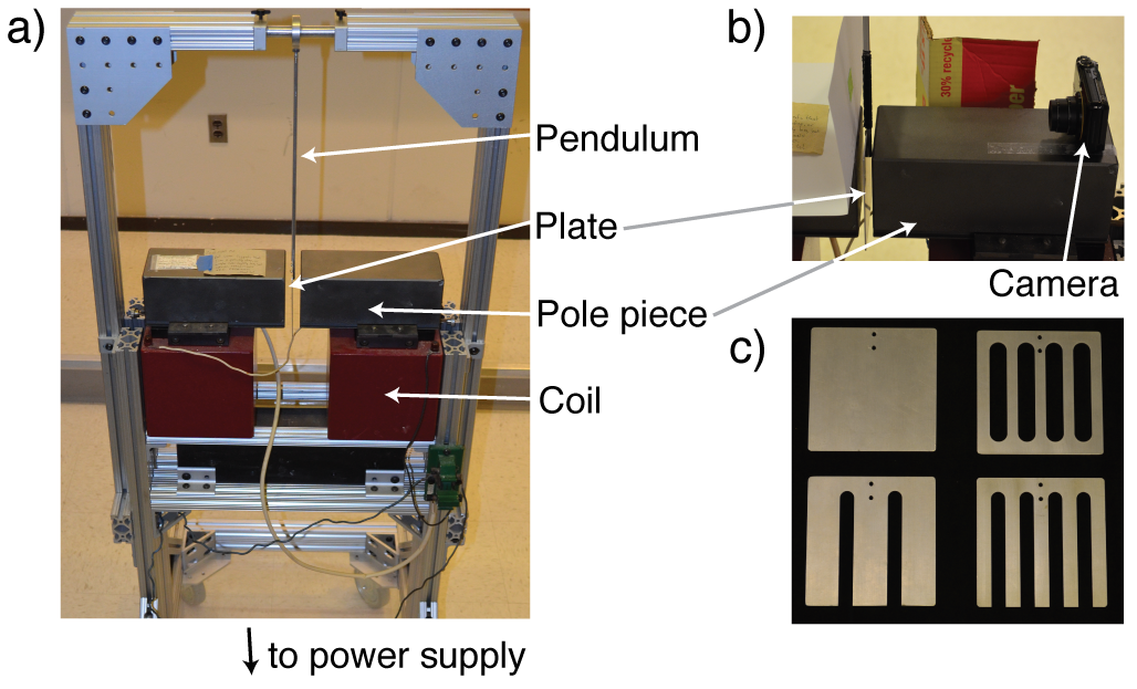
Figure 7: (a) Photograph of the experimental setup, designed as a classroom demonstration for introductory physics. (b) Detail showing placement of camera and screen for imaging. (c) Photograph of paddle shapes used.

In order to test the predictions of the calculations performed in previous sections, we performed an experiment to observe the motion of a pendulum with the different paddles attached and fit the models described in previous sections to the trajectories obtained.

The magnetic brake apparatus used, shown in Figure 7, was designed as a classroom demonstration for introductory physics classes. The apparatus consists of an electromagnet with flat pole pieces of adjustable separation, powered by a 12V car battery. A potential divider and ammeter were incorporated into the circuit so that the current through the magnet could be changed and measured. The pole pieces are $10\times 10$cm and for the present experiment were separated by $2.5$cm. The pendulum hangs from a supporting frame above the pole pieces and is made from a solid rod of length 39.5 cm to which different paddles of interest can be affixed with screws. Four plates were studied, each of side 11.43 cm by 11.43 cm with different arrangements of holes or slits as shown earlier in figure 1(d).

Students collected videos of the motion of the pendulum using a cellphone camera, and in a later iteration a digital camera was used to achieve higher image quality and frame rate. Although data logging hardware could also be used where available, the video approach was adopted as it is inexpensive, required no additional apparatus beyond the existing demonstration and is easily reproduced by others. A white piece of paper with a scale bar was attached to the pole piece behind the camera to provide a uniform background and facilitate quantitative analysis of the resulting videos. The camera was positioned so that the lens was aligned with the rod at rest; its position was marked with chalk so that it could be easily replaced after each trial. The plates were released from the same point outside of the magnet, determined by a ruler placed on top of the pole pieces. The plates were released when the camera started recording and data was collected until the pendulum came to a rest. Two sample frames from one of the movies are shown in figure 8(a). For each plate, 5 videos were collected with $0A$, $0.6A$, $1A$, $1.4A$ and $1.8A$ current flowing through the circuit respectively. Selected videos were taken more than once to verify repeatability. These values obviously depend on the details of the circuit, but were chosen as follows: for the lower bound, a value was sought such that there was a visible difference between the motion of the plate with weakest damping (the one with 4 slits) in the on and off states. For the upper bound, we found a current level such that the plate with the strongest damping gave 2-3 oscillations before coming to a stop, i.e. we are in the oscillatory regime of $\omega>\lambda$ in equation (39).

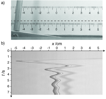
Figure 8: (a) Sample frames from a video of the pendulum’s motion. From this movie, the row of pixels indicated with the dashed line is taken from each frame and composited to produce the resliced image (b).

Having collected the dataset of videos of the pendulum with different plates, the trajectories were extracted from the videos. This was done in two steps: First, the open-source image processing program ImageJ (Schneider et al., 2012) was used to “reslice” the movie, converting it from a stack of images of the $(x,y)$ plane at different time points $t$ to a new stack of images of $(x,t)$ at different vertical positions $y$. An sample output is displayed in fig. 8(b), showing the damped motion of the pendulum as a function of time for the row of the movie indicated by the dashed line in fig. 8(a). The second step in the data extraction was performed by a custom program written in Mathematica, included as Supplementary Material. This first subtracted the background, then for each time point located the position of the bob by finding the centroid of the pixels with intensity above a certain value. The result of this process was to yield for each movie a list of $(x,t)$ representing the trajectory of the pendulum. Using the rulers and known frame rate of the camera (30fps), the list was calibrated to physical coordinates; the program also subtracts the equilibrium position of the pendulum from the $x$ position. To facilitate comparison with the models, the extremum-finding routine mentioned in the previous section was used to identify a list of stationary points $\{(x_{i},t_{i})\}$ from each trajectory. A constant was subtracted from the times such that for each trajectory the first extremum was set to $t=0$.

V Model Comparison

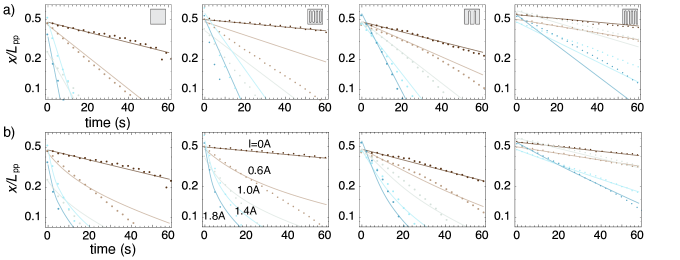
Figure 9: Fits for (a) the simplified wire model and (b) the magneto-quasistatic model. Experimental data is shown as points; the model is shown as lines.

Having obtained a set of experimental trajectories, we now fit both models to the data. Beginning with the simplified wire model, the analytical solution in section III.4 implies that for each individual trajectory the extrema should follow a straight line on semi-log scales with slope

$$\lambda_{wire}=\beta+\left(\frac{A^{2}}{L}\right)\frac{B_{0}^{2}}{\rho}.$$ (44)

From the set of results displayed as points in fig. 9, it is seen that this is generally the case, though some deviations are apparent. In particular, the motion starts to decay more rapidly once $\left|x/L_{pp}\right|\lesssim 0.1$; we therefore excluded this data from our fit. For each plate, several values of current $I$ were used to take a succession of trajectories. Although it is obvious that $B_{0}\propto I$, we did not explicitly measure the magnetic field and therefore absorb this unknown constant of proportionality together with $\rho$ the effective resistivity of the wire into a single fitting parameter $\alpha$. This fitting parameter could, of course, in principle be calculated or measured separately, but the purpose of fitting here is to establish whether the model is consistent with the results for all plates simultaneously. The slopes extracted from the ensemble of plates with different $\Gamma=A^{2}/L$ (calculated values are shown in table 1) at different applied currents $I$ should therefore universally be described by,

$$\lambda_{wire}=\beta+\alpha\Gamma I^{2}.$$ (45)

Estimates for the initial position of each trajectory $x_{0}$ were obtained by fitting a straight line to the extrema individually on semi-log scales. We then estimated $\beta$ for each plate from the $I=0$ trajectory for each plate; the results are shown in table 1. Two pairs of plates seem to cluster around similar values; these were collected at different times indicating that the natural damping of the apparatus, perhaps lubricant in the hinge, changed between them.

	$\Gamma/\Gamma_{square}$	$\beta$	$\alpha$
Square	1	$1.1\times 10^{-2}$	0.060
4 holes	0.441	$4.4\times 10^{-3}$	0.130
2 slits	0.348	$1.2\times 10^{-2}$	0.074
4 slits	0.136	$5.2\times 10^{-3}$	0.044

Table 1: Geometric parameters and fitted $\alpha$, $\beta$ for each plate using the simplified model.

Results from the universal least-squares one-parameter fit for $\alpha$ are shown in fig. 9(a). As can be seen, the fit isn’t bad and follows many of the trajectories quite well. That said, there are many discrepancies. We therefore estimated $\alpha$ from each individual plate using the data at different applied field. While the details of these are not shown here, the quality of fit was very much better. The resultant values of $\alpha$ are displayed in table 1. In particular, it is not surprising that the plate with 4 holes is such an outlier as the wire model cannot account for this geometry. Values for the other plates are the same order of magnitude, which together with fig. 9(a) demonstrates that the simplified model gives reasonable estimates for the influence of plate geometry even though it is based on quite egregious approximations.

In the same spirit, we assume that the damping term in (39) for the magneto-quasistatic model can similarly be described by a universal constant $\alpha$,

$$\lambda_{mqs}(x)=\beta+\alpha P(x)I^{2}.$$

For this model, as well as $x_{0}$, $\beta$, $\alpha$, $P(x)$ and $I$, it is also necessary to specify the natural angular frequency $\omega$; the value from the $I=0$ trajectory for each plate is used since $\beta\ll\omega$ for the weak damping in the absence of the magnetic field and hence $\omega^{\prime}\approx\omega$. The results of the one-parameter universal fit for $\alpha$ are displayed in 9(b). The quality of fit is significantly better, especially for large amplitudes and early times, and more consistent between plates than for the simple model, implying that the magneto-quasistatic model yields good predictions of the effect of plate geometry. Of particular importance is the fact that the fit for the 4 hole plate is no worse than that of the other plates, suggesting that these features have been handled correctly by the model.

Nonetheless, there remains an unexplained phenomenon in the data, i.e the anomalous increase in damping once the amplitude of the motion drops below $x/L_{pp}\sim 0.1$. This is not predicted by either model. The simplified model predicts a constant rate of damping, while the magneto-quasistatic model predicts a crossover from magnetically dominated damping at large amplitudes to Stokes dominated damping at small amplitudes. We tried adjusting the magneto-quasistatic model in various ways—offsetting the position of the plate with respect to the pole pieces and changing the size of the plate relative to the pole pieces—but found no similar effect for any reasonable parameters for the experiment. Clearly, the Stokes form of the non-magnetic damping is most likely at fault, because the source of damping is likely to be primarily the hinge rather than air resistance; further analysis should be performed to determine the origin of this anomaly.

VI Pedagogical Context

The scientific results presented in this paper were obtained in part by students in Spring 2013 as part of the Electromagnetic Theory II class at Tufts University, the second course in the E&M sequence in the graduate program at Tufts; two students from the class are co-authors on the paper (CW and JW) having spent a considerable time subsequently acquiring additional data and performing calculations. In this section, the pedagogical context of these activities is briefly documented in the hope that it is of use to others. The idea of incorporating (simple) experiments in class was motivated by an observation that key scientific skills expected of graduate students—connecting theory and experiment; article reading; journal selection and article preparation—are not included explicitly in the curriculum. The project was spread over the second half of the semester as follows:—

1. A prepatory homework where students derived the magneto-quasistatic model III.

2. Two $1\frac{1}{4}$ hour class periods where students worked in groups. The students were divided into groups of four and worked on: i) conformal mapping analysis, ii) finite element analysis and iii) experiments. The instructor provided scaffolding activities to help students learn FlexPDE and the Schwarz-Christoffel mapping technique. These activities continued subsequently outside of class.

3. A reading activity whereby students had to identify possible journals for publication of this work; this was followed by a 15 minute discussion of journal selection in class.

4. A Just-In-Time Teaching(Novak et al., 1999)-like pre-class activity in which students had to identify the structural elements in a typical paper and construct an outline; these were passed round anonymously for peer feedback.

5. A homework activity in which students prepared an introduction for the paper. Students were asked to read each other’s work and identify strong features as well as possible modifications as a pre-class activity. This was followed by a discussion in class.

6. Each group collaboratively produced a draft section for the final paper as part of a homework; these were combined by TJA into a coherent document and extensively rewritten during the second iteration of experiments.

The focus of the class and restricted time available necessitated some design trade-offs. For example, we chose to use an existing commercial software package, FlexPDE, as opposed to implementing a custom finite element program, for several reasons: First, the scale and complexity of problems solvable with a specialist code is much greater than with a simple custom-written program and hence should be applicable to situations encountered in student’s research projects. Second, the program contains advanced features such as adaptive refinement—allocation of grid points based on estimated error—that are time-consuming to implement. Third, by removing the focus of the exercise from programmatic implementation, time can be spent on understanding how to properly interpret the output using fundamental principles of numerical analysis such as order, error estimation and convergence.

While the project-based approach is well-grounded in a theory of learning (constructivism), due to the small $N=13$ size of the class, it is difficult to rigorously demonstrate the effectiveness of the activity. Future iterations would strongly benefit from pre and post testing. Even so, the outcomes of the project indicate that students made considerable progress towards learning these challenging scientific skills. Moreover, the class was very highly rated in the formal feedback mechanism. It is hoped that, in future, physics education researchers might attempt a thorough analysis of this and related approaches at the graduate level.

VII Conclusion

The present work has provided a careful, quantitative analysis of a familiar classroom demonstration, the van Waltenhofen pendulum. A magneto-quasistatic model has been shown to successfully predict the relative damping of a selection of plates with different geometry using conformal mapping and finite elements as tools to carry out the necessary calculations. As a by-product, a number of valuable resources for more general use, including plots of the current distribution during the course of the motion of the pendulum, have been produced. Additionally, a greatly simplified model, suitable for use in introductory physics classes, has been formulated that could be used to make the classroom demonstration more quantitative.

References

- Babbage and Herschel (1825) C. Babbage and J. F. W. Herschel, Philosophical Transactions of the Royal Society of London 115, 467 (1825).
- Faraday (1832) M. Faraday, Philosophical Transactions of the Royal Society of London 122, 125 (1832).
- von Waltenhofen (1879) A. von Waltenhofen, Taylor & Francis (1879).
- Thompson and Leung (2011) M. Thompson and C. Leung, Physics Education (2011).
- Onorato and Ambrosis (2012) P. Onorato and A. D. Ambrosis, American journal of physics 80, 27 (2012).
- Jackson (1975) J. Jackson, Classical electrodynamics (Wiley, 1975).
- Needham (1999) T. Needham, Visual Complex Analysis (Oxford University Press, USA, 1999).
- Driscoll and Trefethen (2002) T. Driscoll and L. Trefethen, Schwarz-Christoffel Mapping, Cambridge Monographs on Applied and Computational Mathematics (Cambridge University Press, 2002).
- Trefethen (1980) L. N. Trefethen, SIAM Journal on Scientific and Statistical Computing 1, 82 (1980).
- Driscoll (1996) T. A. Driscoll, ACM Trans. Math. Software , 168 (1996).
- Melnikov and Melnikov (2006) Y. Melnikov and M. Melnikov, Engineering Analysis with Boundary Elements 30, 774 (2006).
- Schneider et al. (2012) C. A. Schneider, W. S. Rasband, and K. W. Eliceiri, Nature Materials 9, 671 (2012).
- Novak et al. (1999) G. M. Novak, A. Gavrin, and C. Wolfgang, Just-in-Time Teaching: Blending Active Learning with Web Technology, 1st ed. (Prentice Hall PTR, Upper Saddle River, NJ, USA, 1999).