Quantum Phase Transition and Protected Ideal Transport in a Kondo Chain

Abstract

We study the low energy physics of a Kondo chain where electrons from a one-dimensional band interact with magnetic moments via an anisotropic exchange interaction. It is demonstrated that the anisotropy gives rise to two different phases which are separated by a quantum phase transition. In the phase with easy plane anisotropy, Z₂ symmetry between sectors with different helicity of the electrons is broken. As a result, localization effects are suppressed and the dc transport acquires (partial) symmetry protection. This effect is similar to the protection of the edge transport in time-reversal invariant topological insulators. The phase with easy axis anisotropy corresponds to the Tomonaga-Luttinger liquid with a pronounced spin-charge separation. The slow charge density wave modes have no protection against localizatioin.

Introduction. One-dimensional systems present an ideal platform for formation of charge density waves (CDW) Giamarchi (2004); the transport in clean systems is almost ideal Rosch and Andrei (2000). However, for realistic interactions and at low temperatures, even a weak disorder pins the CDW suppressing the charge transport Giamarchi and Schulz (1988). The ideal transport can be protected by symmetries: a well-known example is the edge transport in two-dimensional time-reversal invariant topological insulators (TIs)Hasan and Kane (2010); Qi and Zhang (2011); Shen (2012); Franz and Molenkamp (2013). The topologically non-trivial state of the bulk and time-reversal symmetry lead to a lock-in relation between the chirality and the spin of edge modes making them helical Wu et al. (2006). As a result, the electron backscattering must be accompanied by a spin-flip; hence the edge transport becomes immune to effects of potential disorder. Other processes which can suppress the ideal transport include scattering by magnetic impurities Tanaka et al. (2011) or inelastic processes due to interactions Schmidt et al. (2012); Cheianov and Glazman (2013); Väyrynen et al. (2013, 2014); Kainaris et al. (2014). All of them become ineffective at low temperatures. The presence of (almost) ballistic edge transport has been confirmed in state-of-the-art experiments König et al. (2007); Roth et al. (2009); Knez et al. (2011); Suzuki et al. (2013). Hence it is accepted that the ballistic transport is protected by time-reversal symmetry and this protection is removed when this symmetry is broken Altshuler et al. (2013); Yevtushenko et al. (2015).

Helical boundary modes can exist in noninteracting systems due to topological nontriviality of the bulk Bernevig and Hughes (2013). In this Letter, we show that helical modes may emerge in interacting systems as a result of spontaneous symmetry breaking. As an illustration, we study a model of Kondo chain Zachar et al. (1996); Honner and Gulacsi (1997); Tsunetsugu et al. (1997); Novais et al. (2002); Gulácsi (2004) consisting of band one-dimensional electrons interacting with local spins; the Hamiltonian of this system is:

$$\hat{H}=-t\sum_{n}\hat{c}^{\dagger}_{n+1}\hat{c}_{n}+\sum_{m}J_{a}\,\hat{c}^{\dagger}_{m}\,\hat{\sigma}^{a}\hat{S}^{a}(m)\,\hat{c}_{m}+H.c.$$ (1)

Here $\,\hat{c}^{\rm T}_{n}\equiv(\hat{c}_{\uparrow}(n),\hat{c}_{\downarrow}(n))\,$ are electron operators at lattice site $\,n$; $\,\hat{\sigma}^{a}\,$ are Pauli matrices ($a=x,y,z$); $\,\hat{S}^{a}(m)$ are components of the spin-s operator located on lattice site $\,m$; $\,t\,$ denotes the overlap integral. It is assumed that sites $\{m\}$ constitute some (not necessarily regular) subset of sites $\{n\}$. We concentrate on the regime of sufficiently high density of spins where the Kondo effect is suppressed and the physics is determined mostly by the Ruderman-Kittel-Kasuya-Yosida (RKKY) interaction NoK . The band is far from half filling, the spins are quantum and the coupling constants are much smaller than the bandwidth, $\,sJ_{a}\ll t$. We will consider the coupling which is isotropic in the $\,XY$-plane: $\,J_{x}=J_{y}\equiv J_{\perp}$.

Brief summary of the results: The low energy (LE) behavior of model (1) includes two distinct regimes corresponding to the easy axis (EA), $J_{z}>J_{\perp}$, and the easy plane (EP), $J_{z}<J_{\perp}$, anisotropy. In the first case, all quasiparticle (fermionic) excitations are gapped. The transport is carried by gapless collective modes, the charge and the spin density waves. The CDW couples to a potential disorder which is able to pin it and to block the charge transport. The SU(2) symmetric point, $J_{z}=J_{\perp}$, is the point of quantum phase transition into a phase with spontaneously broken helicity. In the EP phase at $T=0$, quasiparticles with a given helicity acquire a gap and the other helical branch remains gapless. The charge transport is carried by the gapless helical electrons and by the slow collective excitations (spin-fermion waves). If the spin U(1) symmetry is respected the long range helical ordering makes single-particle backscattering of the gapless modes impossible as in the noninteracting TIs. This leads to suppression of localization effects: the localization radius becomes parametrically large and the dc transport acquires a (partial) symmetry protection in finite but long samples.

Continuum limit: To describe the LE physics we develop a continuum limit theory. This requires to single out smooth modes. We linearize the spectrum of electrons and expand operators $\hat{c}$ in smooth chiral modes:

$$\hat{c}_{\uparrow\downarrow}(n)=\mbox{e}^{-\mbox{i}k_{F}\xi_{0}n}\hat{R}_{\uparrow\downarrow}(x)+\mbox{e}^{\mbox{i}k_{F}\xi_{0}n}\hat{L}_{\uparrow\downarrow}(x),\ x=n\xi_{0}\,;$$ (2)

were $\xi_{0}$ is the lattice constant. The Lagrangian density of the band electrons becomes

$${\cal L}_{\rm e}=\Psi^{\dagger}\Big{[}(\hat{I}\otimes\hat{I})\partial_{\tau}-\mbox{i}(\hat{I}\otimes\hat{\tau}^{z})v_{F}\partial_{x}\Big{]}\Psi.$$ (3)

Here $\tau$ is the imaginary time; the first space in the tensor product is the spin one, the Pauli matrices $\hat{\tau}^{a}$ act in the chiral space; $\hat{I}={\rm diag}(1,1)$; $\,v_{F}=2t\xi_{0}\sin(k_{F}\xi_{0})$ is the Fermi velocity ($\,k_{F}\,$ is the Fermi momentum); $\,\Psi^{\rm T}=\left(R^{\rm T},L^{\rm T}\right)\,$ is the 4-component fermionic spinor field.

Contrary to Ref.Zachar et al. (1996), where the effects of forward scattering at $J_{z}\sim t$ (i.e., of the Kondo physics) were considered, we suggest that the LE physics in the dense limit with $J_{a}\ll t$ (dominated by the RKKY interaction) is governed by backscattering of the fermionic modes. It is described by

$${\cal L}_{\rm bs}=\rho_{s}\sum_{a=x,y,z}J_{a}\sum_{m}\mbox{e}^{2\mbox{i}k_{F}\xi_{0}m}R^{\dagger}S^{a}(m)\hat{\sigma}^{a}L+H.c.$$ (4)

$\rho_{s}$ denotes the dimensionless spin density. ${\cal L}_{\rm bs}$ is expected to lead to opening of the spectral gaps thus reducing the energy of the electrons. As will be clear from the subsequent discussion, the resulting physics is quite different from that of Ref.Zachar et al. (1996).

We can eliminate the oscillatory factors in (4) by absorbing them into the spin configurations which amounts to separation of fast and slow spin variables Hel . The standard parametrization of the spin by azimuthal and polar angles, ${\bf S}=s\{\sin(\theta)\cos(\psi),\sin(\theta)\sin(\psi),\cos(\theta)\}$, with the integration measure ${\cal D}\{\Omega_{S}\}=\sin(\theta){\cal D}\{\theta\}{\cal D}\{\psi\}$ Lwz is not convenient for our purposes. Therefore, we change to the rotating orthonormal basis ${\bf e}_{1,2,3}$ with ${\bf e}_{3}={\bf S}/s$. We define a “longitudinal”, $\roarrow{\cal S}_{\parallel}$, and the “transverse”, $\roarrow{\cal S}_{\perp}$, components of the new spin vector $\roarrow{\cal S}=\roarrow{\cal S}_{\perp}+\roarrow{\cal S}_{\parallel}$ (Fig.1):

$$\frac{\roarrow{\cal S}_{\parallel}}{s}\equiv{\bf e}_{3}\sin\alpha_{\parallel};\,\frac{\roarrow{\cal S}_{\perp}}{s}\equiv[{\bf e}_{1}\cos\alpha_{\perp}+{\bf e}_{2}\sin\alpha_{\perp}]\cos\alpha_{\parallel};$$ (5)

$\alpha_{\perp}=2k_{F}\xi_{0}m+\alpha(x)$. The orthonormality can be resolved by choosing

$${\bf e}_{1} = \{-\cos(\theta)\cos(\psi),-\cos(\theta)\sin(\psi),\sin(\theta)\},$$ (6)

$${\bf e}_{2} = \{\sin(\psi),-\cos(\psi),0\}.$$ (7)

The integration measure for $\alpha,\alpha_{\parallel}$ will be ${\cal D}\{\Omega_{\alpha}\}=\cos(\alpha_{\parallel}){\cal D}\{\alpha_{\parallel}\}{\cal D}\{\alpha\}$, the total measure reads ${\cal D}\{\Omega\}={\cal D}\{\Omega_{\alpha}\}{\cal D}\{\Omega_{S}\}$. This does not result in overcounting the degrees of freedom since we will find a scale separation with two fast (massive $\alpha_{\parallel},\theta$) and two slow (massless $\alpha,\psi$) angles Sca . Verification of the scale separation and stability of the chosen spin configuration will confirm self-consistency of our approach.

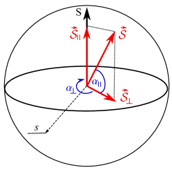
Figure 1: Transformation from the frame of the vector ${\bf S}$ to that of $\roarrow{\cal S}$. Angles $\alpha_{\parallel,\perp}$ define the modulus of the transverse component $\roarrow{\cal S}_{\perp}$ and its rotation around the longitudinal component $\roarrow{\cal S}_{\parallel}$, respectively.

Inserting the new parametrization in Eq.(4) and keeping only the non-oscillatory terms, we find LE Lagrangian ${\cal L}_{\rm eff}={\cal L}_{\rm e}+{\cal L}_{\rm bs}^{\rm(sl)}+{\cal L}_{\rm WZ}$ where

$${\cal L}_{\rm bs}^{\rm(sl)} = \frac{\tilde{s}\rho_{s}}{2}R^{\dagger}\Bigl{\{}J_{\perp}\left[\mbox{e}^{\mbox{i}\psi}\sin^{2}\!\left(\frac{\theta}{2}\right)\hat{\sigma}^{-}\!\!-\mbox{e}^{-\mbox{i}\psi}\cos^{2}\!\left(\frac{\theta}{2}\right)\hat{\sigma}^{+}\right]$$ (9)

$$+J_{z}\sin(\theta)\hat{\sigma}^{z}\Bigr{\}}L\mbox{e}^{-\mbox{i}\alpha}+H.c.;\quad\tilde{s}\equiv s\cos(\alpha_{\parallel});$$

${\cal L}_{\rm WZ}$ is the topological Wess-Zumino term Tsvelik (2003); Sup :

$${\cal L}_{\rm WZ} = \mbox{i}s\rho_{s}\xi_{0}^{-1}\sin(\alpha_{\parallel})[\partial_{\tau}\alpha+\cos(\theta)\partial_{\tau}\psi].$$ (10)

The fermionic gaps become maximal at $\alpha_{\parallel}=0$ and $\theta=0,\pi/2,\pi$. Thus, we expect three extrema of the action whose stability depends on the ratio $J_{\perp}/J_{z}$.

EA anisotropy, $J_{z}>J_{\perp}$: The term $O(J_{z})$ dominates and opens the gap in all fermionic modes. This can be shown straightforwardly after removing the angles $\alpha,\psi$ from the backscattering term (9) by using the Abelian bosonization Gogolin et al. (1998); Fun : we bosonize the fermions and shift bosonic phases:

$$\tilde{\Phi}_{c}=\Phi_{c}-\alpha/2,\ \tilde{\Theta}_{s}=\Theta_{s}-\psi/2.$$ (11)

Here $\Phi_{c}$ and $\Theta_{s}$ are the charge and the (dual) spin phases, their gradients are coupled to charge- and spin source fields, respectively Dua : ${\cal L}_{h}=h_{c}\partial_{x}\Phi_{c}+h_{s}\partial_{x}\Theta_{s}$. After shifting the bosonic phases, terms $\propto h_{c}\partial_{x}\alpha/2$ and $\propto h_{s}\partial_{x}\psi/2$ arise in the Lagrangian. Finally, we can return to the fermionic variables:

$${\cal L}^{\rm(sl)}\simeq{\cal L}_{\rm e}+{\cal L}_{\rm bs}^{\rm(sl)}\!|_{\alpha,\psi=0}+\!\!\!\!\!\!\sum_{2\Phi=\alpha,\psi}\!\!\!\!{\cal L}_{\rm TL}(\Phi,v_{F})+{\cal L}_{\rm WZ}.$$ (12)

Here ${\cal L}_{\rm TL}(\Phi,v)=[(\partial_{\tau}\Phi)^{2}+(v\,\partial_{x}\Phi)^{2}]/\pi v$ is the Lagrangian of the Tomonaga-Luttinger Liquid (TLL), i.e., the anomaly Cro .

For fixed values of $\{\theta,\alpha_{\parallel}\}$, the fermionic spectrum consists of the four Dirac modes with the masses given by:

$$m_{\pm}^{2}=(\tilde{s}\rho_{s}/2)^{2}\left(\sqrt{J^{2}_{\perp}\cos^{2}\theta+J^{2}_{z}\sin^{2}\theta}\pm J_{\perp}\right)^{2}.$$ (13)

Integrating out the gapped fermions, we get the contribution to the ground state energy:

$$E_{\rm GS}=-\frac{\xi_{0}}{2\pi v_{F}}\sum_{\chi=\pm}m_{\chi}^{2}\ln[t/|m_{\chi}|]+o(J_{\perp}^{2},J_{z}^{2}).$$ (14)

If $J_{z}>J_{\perp}$, $E_{\rm GS}$ has minima at $\theta=\pi/2,\alpha_{\parallel}=0$; small fluctuations around the minima read:

$$\delta E_{\rm ea}/{\cal E}\approx(J_{z}^{2}-J_{\perp}^{2})\cos^{2}(\theta)+(J_{z}^{2}+J_{\perp}^{2})\sin^{2}(\alpha_{\parallel}),$$ (15)

where ${\cal E}\equiv\ln\left(t/J\right)(s\rho_{s})^{2}\xi_{0}/4\pi v_{F}$ and we do not distinguish between $J_{z}$ and $J_{\perp}$ in the logarithm. Using Eqs.(10,15) and integrating over the Gaussian fluctuations of the angles, we can find parameters of ${\cal L}_{\rm TL}(\alpha)$ which are renormalized due to the coupling of the spin wave to the gapped fermions: $\,4v_{\alpha}/v_{F}=K_{\alpha}\ll 1$ Lut . The LE Lagrangian for the EA anisotropy is Sub :

$${\cal L}_{\rm ea}={\cal L}_{\rm TL}(\psi,v_{F})/4+{\cal L}_{\rm TL}(\alpha,v_{\alpha})/K_{\alpha}+{\cal L}_{h}^{\rm(ea)}.$$ (16)

${\cal L}_{\rm ea}$ corresponds to two U(1)-symmetric TLL models with the slow charge, $\alpha$, and the fast spin, $\psi$, bosonic modes.

Breaking Z₂ symmetry: If $J_{z}\gg J_{\perp}$, then $m_{+}\simeq m_{-}$, all fermionic modes have (almost) the same gap $\sim J_{z}$, cf. Eq.(9). Mass $m_{-}$ progressively shrinks towards the SU(2) symmetric point of the quantum phase transition where $\,m_{-}=0$ and one subsystem of the helical fermions becomes gapless. Our approach looses its validity at $m_{-}\to 0$. We leave a description of the SU(2) symmetric point for future studies and consider instead the case of the strong EP anisotropy $J_{z}\ll J_{\perp}$.

EP anisotropy, $J_{z}\ll J_{\perp}$: To make the consideration transparent, we put $J_{z}\to 0$ and rewrite Eq.(9) as a sum of helical contributions:

$${\cal L}_{\rm bs}^{\rm(H1)} = \tilde{s}\rho_{s}J_{\perp}R_{\uparrow}^{\dagger}\cos^{2}\left(\theta/2\right)\mbox{e}^{-\mbox{i}(\psi+\alpha)}L_{\downarrow}+H.c.$$ (17)

$${\cal L}_{\rm bs}^{\rm(H2)} = -\tilde{s}\rho_{s}J_{\perp}R_{\downarrow}^{\dagger}\sin^{2}\left(\theta/2\right)\mbox{e}^{\mbox{i}(\psi-\alpha)}L_{\uparrow}+H.c.$$ (18)

If $\,\theta\simeq\pi/2$, both helical sectors have a gap though the coupling constant $J_{\perp}$ is effectively decreased because $\sin^{2}\left(\theta/2\right)\simeq\cos^{2}\left(\theta/2\right)\simeq 1/2$. If $\,\theta\simeq 0,\pi$, only one helical sector acquires the gap $m=m_{+}(J_{z}=0,\alpha_{\parallel}=\theta=0)$, and $\,J_{\perp}\,$ is not suppressed because either $\sin^{2}\left(\theta/2\right)\simeq 1$ or $\cos^{2}\left(\theta/2\right)\simeq 1$. Since the contribution of the gapped fermions to the ground state energy is negative and quadratic in the gap, Eq.(14), we conclude that $\,\theta=\pi/2$ yields maximum of the energy and two (degenerate) minima are $\,\theta=0,\pi$. Thus, the Z₂ symmetry between the helical subsystems is spontaneously broken confirming that the SU(2) symmetric point is the point of a quantum phase transition Dis .

Let us consider the configuration $\theta\simeq 0$ where only ${\cal L}_{\rm bs}^{\rm(H1)}$ yields the femionic gap Sec . One can straightforwardly estimate that contributions of the gapped and the gapless fermions to fluctuations of the ground state energy are of order $\sim(J_{\perp}^{2}/v_{F})\sin^{2}(\theta/2)$ and $\sim(J_{\perp}^{2}/v_{F})\sin^{4}(\theta/2)$, respectively. The latter is subleading, it is beyond our accuracy and must be neglected. Thus, ${\cal L}_{\rm bs}^{\rm(H2)}$ is irrelevant for the effective LE theory and must be neglected too. The combination $\psi-\alpha$ becomes redundant and $\psi$ in the combination $\psi+\alpha$ [see Eqs.(10,17)] can be absorbed in $\alpha$: $\psi+\alpha\to\alpha$ Par . Now, we can proceed very similar to the case of the EA anisotropy: (a) eliminate the shifted spin phase $\alpha$ from ${\cal L}_{\rm bs}^{\rm(H1)}$ with the help of the transformation

$$\tilde{\Phi}_{c}=\Phi_{c}+\alpha/2,\ \tilde{\Theta}_{s}=\Theta_{s}-\alpha/2;$$ (19)

(b) integrate out massive helical fermions and obtain the fermionic energy close to its minima:

$$\delta E_{\rm ep}/{\cal E}\simeq J_{\perp}^{2}[\sin^{2}(\theta/2)+\sin^{2}(\alpha_{\parallel})/2]\,;$$

(c) integrate out small quadratic fluctuations of angles around the stationary value; and (d) bosonize fermions from the gapless helical sector by using the Abelian phase $\Phi_{\rm H}$. These steps yield the effective Lagrangian for the case of the EP Sub :

$${\cal L}_{\rm ep} = {\cal L}_{\rm TL}(\Phi_{\rm H},v_{F})/2+{\cal L}_{\rm TL}(\alpha,v^{\prime}_{\alpha})/K^{\prime}_{\alpha}+{\cal L}_{h}^{\rm(ep)};$$ (20)

where $4v^{\prime}_{\alpha}/v_{F}=K^{\prime}_{\alpha}\ll 1$ Lut . Similar to the EA anisotropy, ${\cal L}_{\rm ep}$ corresponds to two U(1)-symmetric TLL models with the fast, $\Phi_{\rm H}$, and the slow, $\alpha$, bosonic modes. However, as we discuss below, the effective theories with- and without the helical symmetry have different transport properties if a disorder is added.

To conclude this section, we note that Eqs.(17,20) are equivalent to their counterparts describing a helical edge mode in the TI with an array of the Kondo impurities Altshuler et al. (2013); Yevtushenko et al. (2015). In our case, however, this helical mode has emerged as a result of spontaneous symmetry breaking.

Density correlation functions and effects of the disorder: Let us keep source terms for the charge sector: ${\cal L}_{h}^{\rm(ea)}=h_{c}\,\partial_{x}\alpha/2;\ {\cal L}_{h}^{\rm(ep)}=h_{c}(\partial_{x}\Phi_{\rm H}+\partial_{x}\alpha/2)$. The charge density-density correlation function at given frequency and momentum reads as:

$${\cal C}_{\rm ea}\propto Q^{2}\langle\alpha^{*}\alpha\rangle;\ {\cal C}_{\rm ep}\propto Q^{2}\Bigl{(}\langle\Phi_{\rm H}^{*}\Phi_{\rm H}\rangle+\langle\alpha^{*}\alpha\rangle/4\Bigr{)}.$$ (21)

${\cal C}_{\rm ea,ep}$ with Lagrangians ${\cal L}_{\rm ea,ep}$ correspond to the ideal metallic transport. In the EA case, it is supported by the slow CDW with the small compressibility, $K_{\alpha}$. $\,{\cal C}_{\rm ep}\,$ contains the contribution from the helical quasiparticles with the bare velocity and from the slow collective wave with the small compressibility, $K^{\prime}_{\alpha}$ Dru .

The coupling of backscattering spinless impurities to the fermions is described by:

$$V_{\rm dis}[g]=g(x)\Psi^{\dagger}(I\otimes\tau^{\dagger})\Psi+H.c.$$ (22)

Here $g(x)$ is the smooth $2k_{F}$-component of the scalar random potential. We use the model of the Gaussian white noise: $\langle g^{1,2}\rangle_{\rm dis}=0;\langle g(x_{1})g^{*}(x_{2})\rangle_{\rm dis}={\cal D}\delta(x_{1}-x_{2})$, assuming that the disorder is weak, ${\cal D}\ll(m_{\pm},m)v_{F}$, and it cannot change the gaps. After shifts Eq.(11,19), the potential $g$ acquires the phase factor: $g\to g\times\mbox{e}^{\mbox{i}\alpha/2}$. Thus, the backscatterering impurities are coupled to all gapless charge carriers (collective waves and helical fermions).

To figure out whether the disorder may lead to localization, we perform the disorder averaging and integrate out the massive fermions Col . The relevant terms appear only in ${\cal D}^{2}$-order and have a different form in EA and EP phases. In the first case, ${\cal D}^{2}$ couples directly to $\exp(\mbox{i}\alpha)$; in the EP phase, it couples to $R^{+}_{\sigma}L_{-\sigma}\exp(\mbox{i}\alpha)$. The latter fact is related to impossibility of single particle backscattering in the phase with broken helicity. The power counting indicates the parametric difference in the localization radius in both phases: $L^{\rm(loc)}_{\rm ea}/L^{\rm(loc)}_{\rm ep}\sim K_{\alpha}({\cal D}/v_{F}m)^{4/3}\ll 1,$ with $L^{\rm(loc)}_{\rm ep}\sim(v_{F}/m)\left(v_{F}m/{\cal D}\right)^{2}$.

Localization can block the dc transport if a sample size $L$ is large: $L\gg L^{\rm(loc)}$. We thus conclude that the ballistic transport in the phase with broken helical symmetry acquires the symmetry protection up to the parametrically large scale $L^{\rm(loc)}_{\rm ep}$. This conclusion holds true as long as the U(1) symmetry in the spin sector is respected. Breaking the U(1) spin symmetry (e.g. after introducing an anisotropy in the XY-plane) allows the direct backscattering of all fermions and removes protection of the ideal transport in the EP phase [cf. localization of the helical edge modes of the TIs Altshuler et al. (2013) in the absence of the U(1) spin symmetry].

Finite temperature effects in the clean case: All previous calculations have been done for zero temperature, $T=0$. They can be generalized for $T\neq 0$ provided $T$ is smaller than the fermionic gaps. Finite temperature restores a broken helical symmetry at $J_{z}<J_{\perp}$ since thermal fluctuations produce domains with opposite helicity. When the spin configuration interpolates between the phases with different helicity there is an energy increase of the order of the difference between the energy in the unstable state (with $\theta\simeq\pi/2$) and the energy of one of the ground states (with $\theta\simeq 0$ or $\pi$). Thus, we can estimate the energy of the domain wall as $E_{\rm wall}\sim m^{2}\xi_{0}/v_{F}$, cf.Eq.(14). The maximal number of the domain walls in the system of the size $L$ reads as $Lm/v_{F}$. If $T\ll E_{\rm wall}$, it becomes exponentially suppressed: $N_{\rm wall}\sim Lm/v_{F}\exp(-E_{\rm wall}/T)$. If $N_{\rm wall}>1$, the walls appear and block the quasiparticle transport since the electrons with a given helicity are massless only in one domain and massive in the other (neighboring) one. Hence the electrons are reflected from domain boundaries. On the other hand, an influence of the domain wall on the field $\alpha$ is reduced to a jump in the Luttinger parameter $K^{\prime}_{\alpha}$ which cannot affect the dc conductance, cf. Ref.Sedlmayr et al. (2012). Thus, we arrive at the conclusion that the dc transport in the phase with the broken helical symmetry will remain ballistic even at finite temperatures. Temperature effects in the disordered case deserve a separate study because of a complicated interplay between formation of the domain walls and many-body (de)localization of collective waves Basko et al. (2006).

Validity: The effective LE theory, Eqs.(16,20), is valid at energies below the smallest fermionic gap, $m_{-}$ and $m$ for the EA and the EP anisotropy, respectively. Since $m_{-}$ vanishes at the SU(2) symmetric point, the approach fails in the vicinity of the quantum critical point. Quickly oscillating contributions $\propto e^{\pm 2ik_{F}x}$, which we neglected, are generically unable to change the physics at the large distances: If the Kondo chain is close to incommensurability the quickly-oscillating exponentials can be treated as random variables, cf. Ref.Honner and Gulacsi (1997). We note, however, that, in the most interesting case of the broken helical symmetry, the amplitude of the oscillating terms is suppressed in the vicinity of the classical spin configuration, $\theta\simeq 0$, as $\sim(\xi_{0}J_{\perp}^{2}/v_{F})\sin^{4}(\theta/2)$ [see the discussion of the derivation of Eq.(20)] which is squared after averaging over the random fluctuations, i.e., becomes negligible.

Conclusions: We have demonstrated that the dc charge transport in the Kondo chain model (1) with the U(1) symmetry of spins remains ballistic in long samples, $L<L^{\rm(loc)}_{\rm ep}$ even in the presence of the potential disorder when the anisotropy of the exchange interaction is of the easy plane type. Due to the spontaneous breaking of the Z₂ symmetry the current is carried by quasiparticles possessing a particular helicity (i.e. whose spin and chirality are locked) and by composite spin-fermion collective modes. In the presence of the U(1) spin symmetry, all gapless modes are protected from simple backscattering by the mechanism similar to that in noninteracting TIs. We emphasize that the symmetry protected transport in our model results from interaction many-body effects instead of the coupling to the non-interacting and topologically non-trivial bulk. In the case of the easy axis anisotropy, the helical symmetry is respected. The quasiparticles are fully gapped and the transport is carried solely by the collective modes. The slow CDWs do not posses the symmetry protection: the potential disorder can pin them and render the Kondo chain insulating.

Supplemental Materials

.1 1. Derivation of the Wess-Zumino term

Here we discuss the subject of spin action which is usually formulated in the Wess-Zumino form Tsvelik (2003). This form is invariant under rotations, however, it requires an integration over an auxiliary variable which is not convenient for our purposes. We have to find another formulation which would not include the additional integration and, nevertheless, would allow us to change the basis.

Let us start with the spin being defined as ${\bf S}=s\,{\bf e}_{3}$, see the paragraph before Eq.(5) in the main text. Here ${\bf e}_{3}$ is one of vectors from the orthonormal basis ${\bf e}_{1,2,3}$, an example of the vectors ${\bf e}_{1,2}$ is given in Eqs.(6,7). The Wess-Zumino term for this representation is well-known:

$${\cal L}_{\rm WZ}[\theta,\psi]=\frac{\mbox{i}s\rho_{s}}{\xi_{0}}\cos(\theta)\partial_{\tau}\psi\,.$$ (23)

The boundary contribution has been neglected in Eq.(23) and in all equations below since we are interested in smooth (semiclassical) spin modes. We note that Eq.(23) is invariant with respect to all O(2) rotations of the vectors $\,{\bf e}_{1,2}\perp{\bf e}_{3}$:

$${\bf e}_{1}=\cos(\beta)\tilde{{\bf e}}_{1}+\sin(\beta)\tilde{{\bf e}}_{2},\quad{\bf e}_{1}=-\sin(\beta)\tilde{{\bf e}}_{1}+\cos(\beta)\tilde{{\bf e}}_{2}.$$ (24)

This is because $\beta$ is the gauge angle and it either drops out from Eq.(23) (if $\beta={\rm const}$) or yields an unimportant boundary contribution (if $\beta$ depends on time). This allows us to rewrite Eq.(23) by using the vectors $\,{\bf e}_{1,2}\,$ from any orthonormal basis:

$${\cal L}_{\rm WZ}[\theta,\psi]=\frac{\mbox{i}s\rho_{s}}{2\xi_{0}}[({\bf e}_{2},\partial_{\tau}{\bf e}_{1})-({\bf e}_{1},\partial_{\tau}{\bf e}_{2})]=\frac{\mbox{i}s\rho_{s}}{\xi_{0}}({\bf e}_{2},\partial_{\tau}{\bf e}_{1}).$$ (25)

The first equality in Eq.(25) can be verified by direct inspection after inserting expressions (6,7) into Eq.(25) and the second one follows from the orthogonality condition $({\bf e}_{1},{\bf e}_{2})=0$. We note that Eq.(25) contains only scalar products of two vectors and, therefore, it is invariant under the global rotation of the $\{x,y,z\}$-basis:

$$({\bf e}_{j},\partial_{\tau}{\bf e}_{k})=({\bf E}_{j},\partial_{\tau}{\bf E}_{k})\quad\mbox{ if }\quad{\bf E}_{1,2}=\hat{R}_{\rm xyz}\,{\bf e}_{1,2},\quad\hat{R}_{\rm xyz}\hat{R}^{\rm T}_{\rm xyz}=1.$$ (26)

To avoid confusions, subscriptips of orthogonal matrices show the basis where they operate.

Now we change to the new spin, Eq.(5), and define the new orthonormal basis ${\bf e}_{1,23}^{\prime}$ with:

$${\bf e}_{3}^{\prime}\equiv\roarrow{\cal S}/s=\cos({\alpha_{\parallel}})[\cos(\alpha_{\perp}){\bf e}_{1}+\sin(\alpha_{\perp}){\bf e}_{2}]+\sin({\alpha_{\parallel}}){\bf e}_{3}\,.$$ (27)

Two remaining vectors from the new basis can be chosen, for example, as follows:

$${\bf e}_{1}^{\prime} = -\sin({\alpha_{\parallel}})[\cos(\alpha_{\perp}){\bf e}_{1}+\sin(\alpha_{\perp}){\bf e}_{2}]+\cos({\alpha_{\parallel}}){\bf e}_{3},$$ (28)

$${\bf e}_{2}^{\prime} = \sin(\alpha_{\perp}){\bf e}_{1}-\cos(\alpha_{\perp}){\bf e}_{2}.$$ (29)

Let us first assume that $\alpha_{\perp,\parallel}$ does not depend on time. In this simple case, the transformation (27–29) is global in the ${\bf e}_{1,2,3}$ basis but it is local in the $\{x,y,z\}$-basis. The latter statement results from the rotation of the basis vectors ${\bf e}_{1,2,3}$. Thus, before using Eq.(27–29), we have to rewrite Eq.(25) in the form which is invariant under all possible global rotations. Such a form reads as

$${\cal L}_{\rm WZ}[\theta,\psi]=-\frac{\mbox{i}\rho_{s}}{2\xi_{0}}({\bf S},{\bf e}_{i})({\bf e}_{j},\partial_{\tau}{\bf e}_{k})\epsilon_{ijk},$$ (30)

where $\epsilon_{ijk}$ is the antisymmetric tensor. Eq.(30) reduces to Eq.(25) if ${\bf S}=s\,{\bf e}_{3}$. It is clearly invariant under the global rotation by the matrix $\hat{R}_{\rm xyz}$. The invariance under the global rotation by the matrix $\hat{R}_{\rm 123}$ can be easily shown after rewriting the vector ${\bf S}$ in the ${\bf e}_{1,2,3}$-basis, substituting the basis $({\bf e}_{1}^{\prime},{\bf e}_{2}^{\prime},{\bf e}_{3}^{\prime})^{\rm T}=\hat{R}_{\rm 123}({\bf e}_{1},{\bf e}_{2},{\bf e}_{3})^{\rm T}$ into Eq.(30) and using the identity

$$\sum_{i,j,k=1,2,3}[\hat{R}_{\rm 123}]_{ip}\,[\hat{R}_{\rm 123}]_{jm}\,[\hat{R}_{\rm 123}]_{kq}\,\epsilon_{ijk}=\epsilon_{pmq}\,.$$

Following the approach explained in Sect. Continuum limit of the main text, we insert Eqs.(27–29) into Eq.(30) allowing the angles $\alpha_{\perp,\parallel}$ to be the independent variables and substitute $s\,\sin(\alpha_{\parallel}){\bf e}_{3}$ for the spin ${\bf S}$. This procedure yields Eq.(10) in the main text. The second substitution takes into account an effective decrease of the slow component of the spin: after introducing the new rotating frame, the size of the spin will be given by the overlap of this effective spin with the original one, i.e. by $s({\bf e}_{3},{\bf e}_{3}^{\prime})=s\sin(\alpha_{\parallel})$, see Fig.1.

To finalize the discussion of the Wess-Zumino term, we point out a short-cut which allows one to obtain the answer Eq.(10) even faster: we can 1) exploit the gauge invariance described in Eq.(24) and directly insert the vectors ${\bf e}_{1,2}^{\prime}$ into Eq.(25); 2) allow the angles $\alpha_{\perp,\parallel}$ to be independent variables in the actions; 3) do the shift of $\alpha_{\perp}$ and omit the oscillatory terms in ${\cal L}_{\rm WZ}$.

.2 2. Alternative derivation of the effective Lagrangian in the case $J_{z}=0$.

Let us consider the extreme case of the easy plane anisotropy where $J_{z}=0$. Eq.(4) simplifies to

$${\cal L}_{\rm bs}=\rho_{s}J_{\perp}\mbox{e}^{2\mbox{i}k_{F}x}\left(S^{+}R^{\dagger}_{\downarrow}L_{\uparrow}+S^{-}R_{\uparrow}^{\dagger}L_{\downarrow}\right)+H.c.$$ (31)

here $S^{\pm}\equiv S^{x}\pm\mbox{i}S^{y}$. Now we can use the standard parametrization of $\bf S$ by azimuthal and polar angles:

$${\bf S} = s[\sin(P)\cos(A),\sin(P)\sin(A),\cos(P)],$$ (32)

$$\Rightarrow{\cal L}_{\rm bs} = s\rho_{s}J_{\perp}\cos(P)\mbox{e}^{2\mbox{i}k_{F}x}\left(\mbox{e}^{\mbox{i}A}R^{\dagger}_{\downarrow}L_{\uparrow}+\mbox{e}^{-\mbox{i}A}R_{\uparrow}^{\dagger}L_{\downarrow}\right)+H.c.$$ (33)

(notation for the angles are changed as compared to the main text to avoid confusions) and note that the slow spin modes can be easily singled out after a shift

$$A\to A\pm 2k_{F}x.$$ (34)

The choice of the $\pm$ sign substitutes now the choice of the minima (either $\theta=0$ or $\theta=\pi$, see the main text): it breaks the helicity symmetry and corresponds to the strong correlation of the spins to one or the other sector of the helical fermions. The helical sector, which is not correlated with the spins, acquires $4k_{F}$-oscillations and vanishes in the effective Lagrangian for the backscattering. For example, choosing the plus sign, we obtain

$${\cal L}_{\rm bs}^{\rm(H1)}=s\rho_{s}J_{\perp}\cos(P)\mbox{e}^{-\mbox{i}A}R_{\uparrow}^{\dagger}L_{\downarrow}+H.c.,\quad{\cal L}_{\rm bs}^{\rm(H2)}=0;$$ (35)

with the Wess-Zumino term ${\cal L}_{\rm WZ}=\mbox{i}s\rho_{s}\xi_{0}^{-1}\cos(P)\partial_{\tau}A$ and with the integration measure ${\cal D}\{\Omega\}=\sin(P)\,{\cal D}\{P\}{\cal D}\{A\}$. This confirms that the third angle becomes redundant for the effective low-energy theory at $J_{z}=0$.

.3 3. Luttinger parameters $K_{\alpha}$ and $K^{\prime}_{\alpha}$

Calculations described after Eq.(15) of the main text yield the following expressions for the Luttinger parameters:

$$K_{\alpha}\simeq\xi_{0}\frac{\sqrt{J_{z}^{2}+J_{\perp}^{2}}}{\pi v_{F}}\sqrt{\log(t/J)}\ll 1;\quad K^{\prime}_{\alpha}\simeq\frac{4m\xi_{0}}{\pi s\rho_{s}v_{F}}\sqrt{\log(t/m)}\ll\!1.$$ (36)

.4 4. Derivation of the localization radius, $L^{\rm(loc)}$.

In this section, we derive an estimate for the localization radius in the Kondo chain coupled to spinless backscattering impurities. Firstly, we replicate fields

$$V_{\rm dis}[g\,\mbox{e}^{\mbox{i}\alpha/2}]\to\sum_{a}\sum_{\sigma}g\mbox{e}^{\mbox{i}\alpha_{a}/2}R^{\dagger}_{a,\sigma}L_{a,\sigma},\quad\sigma=\uparrow,\downarrow\,;$$ (37)

and calculate the Gaussian integral over the random field $g$. This yields the standard contribution to the action

$$S_{\rm dis}=-\frac{{\cal D}}{2}\int{\rm d}\{x,\tau_{1,2}\}\sum_{a_{1,2}}\sum_{\sigma_{1,2}}\left(\mbox{e}^{\mbox{i}\alpha/2}(R^{\dagger}L)\right)[{\bf 1}]\times\left(\mbox{e}^{-\mbox{i}\alpha/2}(L^{\dagger}R)\right)[{\bf 2}]+H.c.\,,\quad{\bf n}\equiv\{x,\tau_{n},a_{n},\sigma_{n}\}\,,n=1,2\,.$$ (38)

At the next step, we integrate out massive fermions perturbatively by doing an expansion in the small parameter $\,{\cal D}/(m_{\pm},m)v_{F}\ll 1$. Our goal is to find leading terms which can result in pinning of all collective charge carriers (EA and EP phases) and in localization of the massless helical fermions (EP phase). We do it separately for the two different phases.

.4.1 4.1 The EA phase: most relevant terms

Let us put $\,J_{\perp}\to 0\,$ and introduce a spin-dependent fermionic mass $\,m_{\rm ea}(\sigma)=\pm(\tilde{s}\rho_{s}/2)J_{z}\,$ where the plus (minus) correspond to $\,\sigma=\uparrow\,$ ($\sigma=\downarrow$). This allows us to simplify the derivation without loss of generality. The matrix Green’s function for the fermions with a given spin reads:

$$\hat{G}_{m}(\sigma)=\left(G^{(0)}_{R}G^{(0)}_{L}-m_{\rm ea}(\sigma)^{2}\right)^{-1}\left(\begin{array}[]{cc}\left(G^{(0)}_{L}\right)^{-1}&-m_{\rm ea}(\sigma)\\ -m_{\rm ea}(\sigma)&\left(G^{(0)}_{R}\right)^{-1}\end{array}\right);$$ (39)

where $G^{(0)}_{R,L}$ are the Green’s functions of free chiral particles. It is important that $\hat{G}_{m}$ is short ranged and it decays beyond the time scale $1/m_{\rm ea}$ (or beyond the coherence length $\xi_{\rm ea}\equiv v_{f}/m_{\rm ea}$).

Leading terms of the order of $\,O({\cal D}^{1})\,$ are given by $\langle S_{\rm dis}\rangle$ where brackets mean that the massive fermions are integrated out. The corresponding diagrams are shown in Fig.2. It is easy to check that the diagrams from Fig.2-a cancel out after summation over spins indices because $\,m_{\rm ea}(\uparrow)=-m_{\rm ea}(\downarrow)$. The diagrams from Fig.2-b are trivial since $\hat{G}_{m}$ is diagonal in the replica space and the spin phase $\alpha$ is smooth on the scale $1/m_{\rm ea}$; therefore,

$$\mbox{e}^{\mbox{i}\alpha[{\bf 1}]/2}\mbox{e}^{-\mbox{i}\alpha[{\bf 2}]/2}\simeq 1\,,$$ (40)

with some small gradient corrections which are unable to yield pinning.

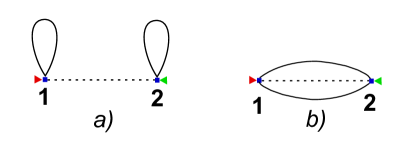
Figure 2: First order diagrams $\,O({\cal D}^{1})\,$ for the EA phase. Red (green) triangulars denote $\,\mbox{e}^{\mbox{i}\alpha/2}\,$ ($\,\mbox{e}^{-\mbox{i}\alpha/2}\,$) with arguments of either the 1st or the 2nd vertex; dashed lines are the disorder correlation functions, solid lines stand for Green’s functions of the massive fermions.

Sub-leading terms of the order of $\,O({\cal D}^{2})\,$ are given by $\langle S_{\rm dis}S_{\rm dis}\rangle$ which generates a lot of diagrams. We leave a detailed analysis for the future and calculate only one typical diagrams which survives after all summations and is able to generate pinning. An example of such a diagram is shown in Fig.3.

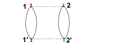
Figure 3: A typical non-trivial diagram, $D^{(2)}_{\rm ea}$, of the order $\,O({\cal D}^{2})\,$ for the EA phase; notations are explained in the caption of Fig.2.

Neglecting unimportant numerical factors, the analytical expression for the diagram from Fig.3 reads as:

$$D^{(2)}_{\rm ea}\propto{\cal D}^{2}\sum_{a_{1,2}}\int{\rm d}\{x,x^{\prime};\tau_{1,2},\tau_{1,2}^{\prime}\}\mbox{e}^{\mbox{i}\left(\alpha[{\bf 1}]-\alpha[{\bf 2}]\right)}\left[\hat{G}_{m}({\bf 1,1^{\prime}})\right]_{1,2}\left[\hat{G}_{m}({\bf 1^{\prime},1})\right]_{1,2}\left[\hat{G}_{m}({\bf 2,2^{\prime}})\right]_{1,2}\left[\hat{G}_{m}({\bf 2^{\prime},2})\right]_{1,2}\,.$$ (41)

Here, we have taken into account the the diagonal structure of $\hat{G}_{m}$ results in $a_{1}=a_{1}^{\prime};a_{2}=a_{2}^{\prime}$ and fused together slow spin phases, for instance: $\alpha[{\bf 1}]+\alpha[{\bf 1^{\prime}}]\simeq 2\alpha[{\bf 1}]$. Now we note that $\hat{G}_{m}({\bf 1,1^{\prime}})=\hat{G}_{m}({\bf 1-1^{\prime}})$ and integrate over all primed variables:

$$D^{(2)}_{\rm ea}\propto\frac{\tilde{{\cal D}}_{0}}{\xi_{\rm ea}^{2}}\sum_{a_{1,2}}\int{\rm d}\{x;\tau_{1,2}\}\mbox{e}^{\mbox{i}\left(\alpha[{\bf 1}]-\alpha[{\bf 2}]\right)}\,;\quad\tilde{{\cal D}}_{0}\equiv{\cal D}\left(\frac{{\cal D}}{v_{F}m_{\rm ea}}\right).$$ (42)

The structure of Eq.(42) corresponds to the disordered Sine-Gordon model which appears in the theory of the usual TLL Giamarchi (2004). The effective disorder strength $\tilde{{\cal D}}$ is renormalized and obeys the well-known RG equation Giamarchi and Schulz (1988):

$${\mbox{E}A}:\quad\partial_{\log}\log(\tilde{{\cal D}})=3-2K_{\alpha}\simeq 3\,,\quad\tilde{{\cal D}}(\xi_{\rm ea})=\tilde{{\cal D}}_{0}\,;$$ (43)

the second equality of Eq.(43) has been obtained by using Eq.(36).

.4.2 4.2 The EP phase: most relevant terms

We start again from the leading diagrams generated by $\langle S_{\rm dis}\rangle$. The principal difference of the EP phase from the EA one is that the matrix Green’s function, Eq.(39), corresponds now to the massive fermions with a given helicity. This changes the structure of the first order diagram, see Fig.4. All these diagrams correspond to forward-scattering of the massless helical fermions and they contain only small gradients of the phase $\,\alpha$, cf. Eq.(40) and its explanation. Thus, the leading diagrams are trivial and they cannot yield localization, the sub-leading diagrams must be considered.

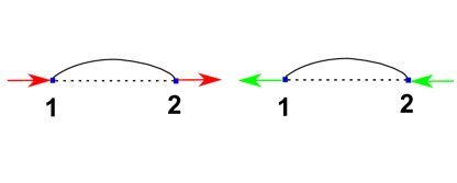
Figure 4: Two typical examples of first order diagrams $\,O({\cal D}^{1})\,$ for the EP phase. Incoming red (green) arrows denote the product of smooth fields $\,\mbox{e}^{\mbox{i}\alpha/2}L_{\uparrow}\,$ ($\,\mbox{e}^{-\mbox{i}\alpha/2}R_{\downarrow}\,$) with arguments of either the 1st or the 2nd vertex; outgoing arrows denote the conjugated product, dashed lines are the disorder correlation functions, solid lines stand for Green’s functions of the massive helical fermions.

$\langle S_{\rm dis}S_{\rm dis}\rangle$ generates 16 diagrams with back-scattering of the massless fermions and exponentials of the phase $\alpha$ which do not cancel, see Fig.5

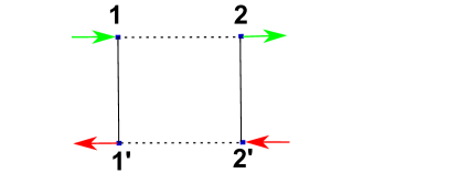
Figure 5: A typical non-trivial diagram, $D^{(2)}_{\rm ep}$, of the order $\,O({\cal D}^{2})\,$ for the EP phase; notations are explained in the caption of Fig.4.

Neglecting unimportant numerical factors, the analytical expression for the diagram from Fig.5 reads as:

$$D^{(2)}_{\rm ep}\propto{\cal D}^{2}\sum_{a_{1,2}}\int{\rm d}\{x,x^{\prime};\tau_{1,2},\tau_{1,2}^{\prime}\}\mbox{e}^{\mbox{i}\left(\alpha[{\bf 1}]-\alpha[{\bf 2}]\right)}\,L^{\dagger}_{\downarrow}[{\bf 2}]R^{\dagger}_{\uparrow}[{\bf 1}]\,L_{\downarrow}[{\bf 1}]R_{\uparrow}[{\bf 2}]\,\left[\hat{G}_{m}({\bf 1,1^{\prime}})\right]_{1,2}\left[\hat{G}_{m}({\bf 2,2^{\prime}})\right]_{1,2}\,;$$ (44)

see explanations after Eq.(41) and note the $m$ must be substituted for $m_{\rm ea}(\sigma)$ in $\hat{G}_{m}$. Calculating integrals over all primed variables, we find:

$$D^{(2)}_{\rm ep}\propto\bar{{\cal D}}_{0}\sum_{a_{1,2}}\int{\rm d}\{x;\tau_{1,2}\}\mbox{e}^{\mbox{i}\left(\alpha[{\bf 1}]-\alpha[{\bf 2}]\right)}\,L^{\dagger}_{\downarrow}[{\bf 2}]R^{\dagger}_{\uparrow}[{\bf 1}]\,L_{\downarrow}[{\bf 1}]R_{\uparrow}[{\bf 2}]\,,\quad\bar{{\cal D}}_{0}\equiv{\cal D}\left(\frac{{\cal D}}{v_{F}m}\right).$$ (45)

This equation also can be reduced to the form of Eq.(42) if remaining fermions are bosonized and we explicitly single out new charge- and spin- density waves. However, the RG equation for $\bar{{\cal D}}$ can be obtained without such a complicated procedure with the help of the power counting. Firstly we note that the scaling dimension of each back-scattering term in Eq.(45), $L^{\dagger}R$ and $R^{\dagger}L$, is 1. The anomalous dimension of each exponential, $\mbox{e}^{\pm\mbox{i}\alpha}$, is $K_{\alpha}^{\prime}\ll 1$. The normal dimension in Eq.(45) is 3 which comes from three-fold integral. Combining these dimensions together and neglecting small $K_{\alpha}^{\prime}$, we find

$${\mbox{E}P}:\quad\partial_{\log}\log(\bar{{\cal D}})=3-2\times 1+O(K_{\alpha})\simeq 1\,;\quad\bar{{\cal D}}(\xi_{\rm ep})=\bar{{\cal D}}_{0}\,,\ \xi_{\rm ep}=v_{F}/m\,.$$ (46)

.4.3 4.3 Comparison of the localization radius in different phases

The solution of the RG equations, Eqs.(43,46), reads as

$$\tilde{\cal D}(x)=\tilde{\cal D}_{0}\left(\frac{x}{\xi_{\rm ea}}\right)^{3},\quad\bar{\cal D}(x)=\bar{\cal D}_{0}\frac{x}{\xi_{\rm ep}}\,;$$ (47)

with $\xi_{\rm ep}=v_{F}/m$. The localization radius is defined as a scale on which the renormalized disorder becomes of the order of the cut-off:

$$\tilde{\cal D}\left(L^{\rm(loc)}_{\rm ea}\right)=K_{\alpha}v_{\alpha}^{2}/\xi_{\rm ea}\sim K_{\alpha}^{3}v_{F}^{2}/\xi_{\rm ea}\,;\quad\bar{\cal D}\left(L^{\rm(loc)}_{\rm ep}\right)=v_{F}^{2}/\xi_{\rm ep}\,.$$ (48)

The additional small factor $K_{\alpha}$ is the equation for $L^{\rm(loc)}_{\rm ea}$ can be justified with the help of the standard optimization procedure Giamarchi (2004) where $L^{\rm(loc)}\,$ is defined as a spatial scale on which the typical potential energy of the disorder becomes equal to the energy governed by the term $\,\propto(\partial_{x}\alpha)^{2}\,$ in the Lagrangian ${\cal L}_{\rm ea}$, Eq.(16).

Definitions Eq.(48) result in

$$L^{\rm(loc)}_{\rm ea}\sim\xi_{\rm ea}K_{\alpha}\left(\frac{v_{F}^{2}}{\xi_{\rm ea}\tilde{\cal D}_{0}}\right)^{1/3}\!\!\!\sim\xi_{\rm ea}K_{\alpha}\left(\frac{v_{F}m_{\rm ea}}{{\cal D}}\right)^{2/3}\!\!\!;\quad L^{\rm(loc)}_{\rm ep}\sim\frac{v_{F}^{2}}{\bar{\cal{D}}_{0}}\sim\xi_{\rm ep}\left(\frac{v_{F}m}{{\cal D}}\right)^{2}\,.$$ (49)

Assuming $\xi_{\rm ea}\sim\xi_{\rm ep}$ and $m_{\rm ea}\sim m$, we obtain

$$\frac{L^{\rm(loc)}_{\rm ea}}{L^{\rm(loc)}_{\rm ep}}\sim K_{\alpha}\left(\frac{{\cal D}}{v_{F}m}\right)^{4/3}\ll 1\,.$$ (50)

This demonstrates that the strong suppression of localization can occur in the EP phase where the helical symmetry is broken.

We note in passing that the scaling exponent of $\bar{\cal D}(x)$ is the same as in the case of non-interacting 1d fermions but suppression of localization in the EP phase is reflected by the additional large factor $v_{F}m/{\cal D}$ in the expression for the localization radius $L^{\rm(loc)}_{\rm ep}$.

References

Giamarchi (2004)T. Giamarchi, Quantum physics in
one dimension (Clarendon; Oxford University
Press, Oxford, 2004).
Rosch and Andrei (2000)A. Rosch and N. Andrei, Phys. Rev. Lett. 85, 1092 (2000).
Giamarchi and Schulz (1988)T. Giamarchi and H. J. Schulz, Phys. Rev. B 37, 325 (1988).
Hasan and Kane (2010)M. Z. Hasan and C. L. Kane, Rev.
Mod. Phys. 82, 3045
(2010).
Qi and Zhang (2011)X. L. Qi and S. C. Zhang, Rev. Mod. Phys. 83, 1057 (2011).
Franz and Molenkamp (2013)M. Franz and L. Molenkamp, Topological
Insulators (Elsevier Science, 2013).
Wu et al. (2006)C. Wu, B. A. Bernevig, and S. C. Zhang, Phys. Rev. Lett. 96, 106401 (2006).
Tanaka et al. (2011)Y. Tanaka, A. Furusaki, and K. A. Matveev, Phys. Rev. Lett. 106, 236402 (2011).
Schmidt et al. (2012)T. L. Schmidt, S. Rachel,
F. von Oppen, and L. I. Glazman, Phys. Rev. Lett. 108, 156402 (2012).
Cheianov and Glazman (2013)V. Cheianov and L. I. Glazman, Phys. Rev. Lett. 110, 206803
(2013).
Väyrynen et al. (2013)J. I. Väyrynen, M. Goldstein, and L. I. Glazman, Phys. Rev. Lett. 110, 216402
(2013).
Väyrynen et al. (2014)J. I. Väyrynen, M. Goldstein, Y. Gefen, and L. I. Glazman, PRB 90, 115309 (2014).
Kainaris et al. (2014)N. Kainaris, I. V. Gornyi, S. T. Carr, and A. D. Mirlin, Phys. Rev. B 90, 075118 (2014).
König et al. (2007)M. König, S. Wiedmann,
C. Brune, A. Roth, H. Buhmann, L. W. Molenkamp, X. L. Qi, and S. C. Zhang, Science 318, 766 (2007).
Roth et al. (2009)A. Roth, C. Brüne,
H. Buhmann, L. W. Molenkamp, J. Maciejko, X.-L. Qi, and S.-C. Zhang, Science 325, 294 (2009).
Knez et al. (2011)I. Knez, R.-R. Du, and G. Sullivan, Phys. Rev. Lett. 107, 136603 (2011).
Suzuki et al. (2013)K. Suzuki, Y. Harada,
K. Onomitsu, and K. Muraki, Phys. Rev. B 87, 235311 (2013).
Altshuler et al. (2013)B. L. Altshuler, I. L. Aleiner, and V. I. Yudson, Phys. Rev. Lett. 111, 086401 (2013).
Yevtushenko et al. (2015)O. M. Yevtushenko, A. Wugalter, V. I. Yudson, and B. L. Altshuler, “Transport in
helical Luttinger Liquid with Kondo impurities,” (2015), arXiv:1503.03348.
Bernevig and Hughes (2013)B. A. Bernevig and T. L. Hughes, Topological insulators
and topological superconductors (Princeton
University Press, 2013).
Zachar et al. (1996)O. Zachar, S. A. Kivelson, and V. J. Emery, Phys. Rev. Lett. 77, 1342 (1996).
Honner and Gulacsi (1997)G. Honner and M. Gulacsi, Phys. Rev. Lett. 78, 2180 (1997).
Tsunetsugu et al. (1997)H. Tsunetsugu, M. Sigrist,
and K. Ueda, Rev. Mod. Phys. 69, 809 (1997).
Novais et al. (2002)E. Novais, E. Miranda,
A. H. Castro Neto, and G. G. Cabrera, Phys. Rev. B 66, 174409 (2002).
(27)This statement means that the spin density
is sufficiently high so that the Kondo effect is cut by the gap generated by
backscattering terms in , cf. Refs.Altshuler et al. (2013); Yevtushenko et al. (2015). It
holds true when the gap exceeds the Kondo temperature.
(28)This approach is supported by numerical
studies of the Kondo chain of classical spins which indicate that the phase
diagram of the system reflects helical spin configurations
Hu et al. (2015). The physics, which is governed by the helical effects
in spins, is also studied in
Refs.Braunecker et al. (2009); Klinovaja et al. (2013); Choy et al. (2011).
(29)The topological Wess-Zumino term (the Berry
phase), , must be added to the Lagrangian
Tsvelik (2003).
(30)We note that the procedure of separation of
slow and fast variables is standard and is routinely used in RG calculations:
see, for example, Chapter 1 in Ref.Tsvelik (2003).
Tsvelik (2003)A. M. Tsvelik, Quantum Field Theory in
Condensed Matter Physics (Cambridge: Cambridge
University Press, 2003).
(32)Derivation of Eq.(10) is explained in
Suppl.Mat. No.1.
Gogolin et al. (1998)A. O. Gogolin, A. A. Nersesyan, and A. M. Tsvelik, Bosonization and
strongly correlated systems (Cambridge: Cambridge
University Press, 1998).
(34)Alternatively, one can do gauge
transformations of the fermionic fields and obtaine an anomaly from the
Jacobian Grishin et al. (2004).
(35)Two remaining fields can be integrated
out.
(36)While deriving Eq.(12), we
have neglected the gradient coupling of the fermions and the spin phases, , which is justified for
energies below the fermion gaps.
(37)Expressions for the Luttinger parameters and are given Suppl.Mat. No.3.
(38)While deriving Eqs.(16) and
(20), we have neglected in the subleading
terms and
,
respectively. This is justified for energies below the fermion
gaps.
(39)We note that helicity is given by the
product of the spin projection and the electron velocity, . Hence, helical symmetry is discrete and it can be
spontaneously broken in one dimension at . The corresponding order
parameter is related to the average : in the phase with the broken symmetry
and
otherwise.
(40)The second minima can
be considered similarly and it yields the same effective Lagrangian , Eq.(20).
(41)One can arrive at the same conclusion even
faster using the standard parametrization of , see Suppl.Mat.
No.2.
(42)The small compressibility of the bosonic
modes leads to suppression of the Drude weight which reflects the coupling of
the spin waves to the gapped fermions Altshuler et al. (2013).
(43)All essential details of this calculus are
presented in Suppl.Mat. No.4.
Sedlmayr et al. (2012)N. Sedlmayr, J. Ohst,
I. Affleck, J. Sirker, and S. Eggert, Phys. Rev. B 86, 121302 (2012).
Basko et al. (2006)D. M. Basko, I. L. Aleiner,
and B. L. Altshuler, Annals of
Physics 321, 1126
(2006).
Hu et al. (2015)W. Hu, R. T. Scalettar, and R. R. P. Singh, “Interplay of magnetic order,
pairing and phase separation in a one dimensional spin fermion model,”
(2015), arXiv:1506.04809.
Braunecker et al. (2009)B. Braunecker, P. Simon, and D. Loss, Phys. Rev. B 80, 165119 (2009).
Klinovaja et al. (2013)J. Klinovaja, P. Stano,
A. Yazdani, and D. Loss, Phys. Rev. Lett. 111, 186805 (2013).
Choy et al. (2011)T.-P. Choy, J. M. Edge,
A. R. Akhmerov, and C. W. J. Beenakker, Phys. Rev. B 84, 195442 (2011).
Grishin et al. (2004)A. Grishin, I. V. Yurkevich, and I. V. Lerner, Phys. Rev. B 69, 165108 (2004).