Mining Mid-level Visual Patterns with Deep CNN Activations

Abstract

The purpose of mid-level visual element discovery is to find clusters of image patches that are representative of, and which discriminate between, the contents of the relevant images. Here we propose a pattern-mining approach to the problem of identifying mid-level elements within images, motivated by the observation that such techniques have been very effective, and efficient, in achieving similar goals when applied to other data types. We show that CNN activations extracted from image patches typical possess two appealing properties that enable seamless integration with pattern mining techniques. The marriage between CNN activations and a pattern mining technique leads to fast and effective discovery of representative and discriminative patterns from a huge number of image patches, from which mid-level elements are retrieved. Given the patterns and retrieved mid-level visual elements, we propose two methods to generate image feature representations. The first encoding method uses the patterns as codewords in a dictionary in a manner similar to the Bag-of-Visual-Words model. We thus label this a Bag-of-Patterns representation. The second relies on mid-level visual elements to construct a Bag-of-Elements representation. We evaluate the two encoding methods on object and scene classification tasks, and demonstrate that our approach outperforms or matches the performance of the state-of-the-arts on these tasks.

keywords: Mid-level visual element discovery, pattern mining, convolutional neural networks

1 Introduction

Image patches that capture important aspects of objects are crucial to a variety of state-of-the-art object recognition systems. For instance, in the Deformable Parts Model (DPM) [31] such image patches represent object parts that are treated as latent variables in the training process. In Poselets [12], such image patches are used to represent human body parts, which have been shown to be beneficial for human detection [10] and human attribute prediction [11] tasks. Yet, obtaining these informative image patches in both DPM and Poselets require extensive human annotations (DPM needs object bounding boxes while the Poselets model needs the information of human body keypoints). Clearly, the discovery of these representative image patches with minimal human supervision would be desirable. Studies on mid-level visual elements (a.k.a, mid-level discriminative patches) offer one possible solution to this problem.

Mid-level visual elements are clusters of image patches discovered from a dataset where only image labels are available. As noted in the pioneering work of [80], such patch clusters are suitable for interpretation as mid-level visual elements only if they satisfy two requirements, i.e., representativeness and discriminativeness. Representativeness requires that mid-level visual elements should frequently occur in the images with same label (i.e., target category), while discriminativeness implies that they should be seldom found in images not containing the object of interest. For instance, image patches containing the wheel of a car may be a mid-level visual element for the car category, as most car images contain wheels, and car wheels are seldom found in images of other objects (this implies also that they are visually distinct from other types of wheels). The discovery of mid-level visual elements has boosted performance in a variety of vision tasks, such as image classification [80, 50, 24] and action recognition [47, 91].

As another line of research, pattern mining techniques have also enjoyed popularity amongst the computer vision community, including image classification [95, 32, 33, 87], image retrieval [34] and action recognition  [39, 38], largely to due to their capability of discovering informative patterns hidden inside massive of data.

In this paper, we address mid-level visual element discovery from a pattern mining perspective. The novelty in our approach of is that it systematically brings together Convolutional Neural Networks (CNN) activations and association rule mining, a well-known pattern mining technique. Specifically, we observe that for an image patch, activations extracted from fully-connected layers of a CNN possess two appealing properties which enable their seamless integration with this pattern mining technique. Based on this observation, we formulate mid-level visual element discovery from the perspective of pattern mining and propose a Mid-level Deep Pattern Mining (MDPM) algorithm that effectively and efficiently discovers representative and discriminative patterns from a huge number of image patches. When we retrieve and visualize image patches with the same pattern, it turns out that they are not only visually similar, but also semantically consistent (see by way of example the game in Fig. 1 and then check your answers below).

Relying on the discovered patterns and retrieved mid-level visual elements, we propose two methods to generate image features for each of them (Sec. 5). For the first feature encoding method, we compute a Bag-of-Patterns representation which is motivated by the well-known Bag-of-Visual-Words representation [81]. For the second method, we first merge mid-level visual elements and train detectors simultaneously, followed by the construction of a Bag-of-Elements representation. We evaluate the proposed feature representations on generic object and scene classification tasks. Our experiments demonstrate that the classification performance of the proposed feature representation not only outperforms all current methods in mid-level visual element discovery by a noticeable margin with far fewer elements used, but also outperform or match the performance of state-of-the-arts using CNNs for the same task.

In summary, the merits of the proposed approach can be understood from different prospectives.

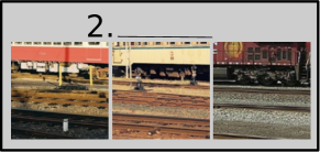
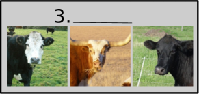
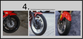
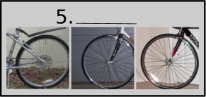
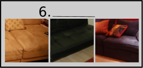
Figure 1: Name that Object: Given the mid-level visual elements discovered by our algorithm from the Pascal VOC 2007 dataset, can you guess what categories are they from?

• Efficient handling of massive image patches. As noted by [24], one of the challenges in mid-level visual element discovery is the massive amount of random sampled patches to go through. However, pattern mining techniques are designed to handle large data sets, and are extremely capable of doing so. In this sense, if appropriately employed, pattern mining techniques can be a powerful tool for overcoming this data deluge in mid-level visual element discovery.

• A straightforward interpretation of representativness and discriminativeness. In previous works on mid-level visual element discovery, different methods have been proposed for interpreting the dual requirements of representativeness and discriminativeness. Here in this work, interpreting these two requirements in the pattern mining terminology is straightforward. To our knowledge, we are the first to formulate mid-level visual element discovery from the perspective of pattern mining.

• Feature encoder of CNN activations of image patches. Recent state-of-the-art results on many image classification tasks (e.g., indoor scene, object, texture) are achieved by applying classical feature encoding methods [69, 48] on the top of CNN activations of image patches [42, 18, 17]. In our work, we demonstrate that mid-level visual elements, which are discovered by the proposed MDPM algorithm, can also be a good alternative feature encoder for CNN activations of image patches.

The remainder of the paper is organized as follows. In Sec. 2, we review some of the related work on mid-level visual element discovery as well as relevant vision applications. In Sec. 3 we explain some of the relevant pattern mining terminology and how pattern mining techniques have been successfully applied to computer vision tasks previously. The details of our MDPM algorithm are provided in Sec. 4. In particular, we start by introducing two desirable properties of CNN activations extracted from image patches (Sec. 4.1), which serve as the cornerstones of the proposed MDPM algorithm. In Sec. 5, we apply the discovered patterns and mid-level visual elements to generate image feature representations, followed by extensive experimental validations in Sec. 6. Some further discussions are presented in Sec. 7 and we conclude the paper in Sec. 8.

Preliminary results of this work appeared in [55]. In this paper, we extend [55] in the following aspects. Firstly, for the theory part, we propose a new method to generate image representations using the discovered patterns (i.e., the Bag-of-Patterns representation). Furthermore, more extensive experiment are presented in this manuscript, such as more detailed analysis of different components of the proposed framework. Last but not least, we present a new application of mid-level visual elements, which is the analysis of the role of context information using mid-level visual elements (Sec. 6.4). At the time of preparing of this manuscript, we are aware of at least two works [22, 65] which are built on our previous work [55] in different vision applications, including human action and attribute recognition [22] and modeling visual compatibility [65], which reflects that our work is valuable to the computer vision community. Our code is available at https://github.com/yaoliUoA/MDPM.

2 Related work

2.1 Mid-level visual elements

Mid-level visual features have been widely used in computer vision, which can be constructed by different methods, such as supervised dictionary learning [13], hierarchically encoding of low-level descriptors [1, 78, 33] and the family of mid-level visual elements [80, 50, 24]. As the discovery of mid-level visual elements is the very topic of this paper, we mainly discuss previous works on this topic.

Mid-level visual element discovery has been shown to be beneficial to image classification tasks, including scene categorization [80, 24, 50, 83, 54, 92, 9, 67, 55, 62] and fine-grained categorization [93]. For this task, there are three key steps, (1) discovering candidates of mid-level visual elements, (2) selecting a subset of the candidates, and finally (3) generating image feature representations.

In the first step, various methods have been proposed in previous work to discover candidates of mid-level visual elements in previous works. Usually starting from random sampled patches which are weakly-labeled (e.g., image-level labels are known), candidates are discovered from the target category by different methods, such as cross-validation training patch detectors [80], training Exemplar LDA detectors [50], discriminative mode seeking [24], minimizing a latent SVM object function with a group sparsity regularizer [83, 84], and the usage of Random Forest [9]. In this work, we propose a new algorithm for discovering the candidates from a pattern mining perspective (Sec. 4).

The goal of the second step is to select mid-level visual elements from a large pool of candidates, which can best interpret the requirements of representative and discriminative. Some notable criteria in previous includes a combination of purity and discriminativeness scores [80], entropy ranking  [50, 53]. the Purity-Coverage plot [24] and the squared whitened norm response  [4, 5]. In our work, we select mid-level visual elements from the perspective of pattern selection (Sec. 5.1.1) and merging (Sec. 5.2.1).

As for the final step of generating image feature representation for classification, most previous works [80, 50, 24] follow the same principle, that is, the combination of maximum detection scores of all mid-level elements from different categories in a spatial pyramid [52]. This encoding method is also adopted in our work (Sec. 5.2.2).

In addition to image classification, some works apply mid-level visual elements to other vision tasks as well, including visual data mining [25, 74], action recognition [47, 91], discovering stylistic elements [53], scene understanding [35, 66, 36], person re-identification [99], image re-ranking [20], weakly-supervised object detection [82]. In object detection, before the popularity of R-CNN [41], approaches on object detection by learning a collection of mid-level detectors are illustrated by [27, 76, 7].

2.2 Pattern mining in computer vision

Pattern mining techniques, such as frequent itemset mining and its variants, have been studied primarily amongst the data mining community, but a growing number of applications can be found in the computer vision community.

Early works have used pattern mining techniques in object recognition tasks, such as finding frequent co-occurrent visual words [97] and discovering distinctive feature configurations [70]. Later on, for recognizing human-object interactions, [95] introduce ‘gouplets’ discovered in a pattern mining algorithm, which encodes appearance, shape and spatial relations of multiple image patches. For 3D human action recognition, discriminative actionlets are discovered in a pattern mining fashion [89]. By finding closed patterns from local visual word histograms, [32, 33] introduce Frequent Local Histograms (FLHs) which can be utilized to generate new image representation for classification. Another interesting work is [87] in which images are represented by histograms of pattern sets. Relying on a pattern mining technique,  [34] illustrate how to address the image retrieval problem using mid-level patterns. More recently, [74] design a method for summarizing image collections using closed patterns. Pattern mining techniques have been also successfully applied to some other vision problems, such as action recognition in videos  [39, 38].

For the image classification task, most of the aforementioned works are relying on hand-crafted features, especially Bag-of-visual-words [81], for pattern mining. In contrast, to our knowledge, we are first to describe how pattern mining techniques can be combine with the state-of-the-art CNN features, which have been widely applied in computer vision nowadays. Besides, our work can be viewed as a new application of pattern mining techniques in vision, that is, the discovery of mid-level visual elements.

3 Background on pattern mining

3.1 Terminology

Originally developed for market basket analysis, frequent itemset and association rule are well-known terminologies within data mining. Both might be used in processing large numbers of customer transactions to reveal information about their shopping behaviour, for example.

More formally, let $A=\{a_{1},a_{2},\ldots,a_{M}\}$ denote a set of $M$ items. A transaction $T$ is a subset of $A$ (i.e., $T\subseteq A$) which contains only a subset of items ($|T|\ll M$). We also define a transaction database $\mathcal{D}=\{T_{1},T_{2},\ldots,T_{N}\}$ containing $N$ (typically millions, or more) transactions. Given these definitions, the frequent itemset and association rule are defined as follows.

Frequent itemset. A pattern $P$ is also a subset of $A$ (i.e., itemset). We are interested in the fraction of transactions $T\in\mathcal{D}$ which contain $P$. The support of $P$ reflects this quantity:

$${\mathrm{supp}}(P)=\frac{|\{T|T\in\mathcal{D},P\subseteq T\}|}{N}\in[0,1],$$ (1)

where $|\cdot|$ measures the cardinality. $P$ is called a frequent itemset when ${\mathrm{supp}}(P)$ is larger than a predefined threshold.
Association rule. An association rule $I\rightarrow{a}$ implies a relationship between pattern $P$ (antecedents) and an item ${a}$ (consequence). We are interested in how likely it is that ${a}$ is present in the transactions which contain $P$ within $\mathcal{D}$ . In a typical application this might be taken to imply that customers who bought items in $P$ are also likely to buy item ${a}$, for instance. The confidence of an association rule ${\mathrm{conf}}(P\rightarrow{a})$ can be taken to reflect this probability:

$$\begin{split}{\mathrm{conf}}(P\rightarrow{a})&=\frac{{\mathrm{supp}}(P\cup\{{a}\})}{{\mathrm{supp}}(P)}\\ &=\frac{|\{T|T\in\mathcal{D},(P\cup\{{a}\})\subseteq T\}|}{|\{T|T\in\mathcal{D},P\subseteq T\}|}\in[0,1].\end{split}$$ (2)

In practice, we are interested in “good” rules, meaning that the confidence of these rules should be reasonably high.

A running example. Consider the case when there are $4$ items in the set (i.e., $A=\{a_{1},a_{2},a_{3},a_{4}\}$) and $5$ transactions in $\mathcal{D}$,

• $T_{1}=\{a_{3},a_{4}\}$,

• $T_{2}=\{a_{1},a_{2},a_{4}\}$,

• $T_{3}=\{a_{1},a_{4}\}$,

• $T_{4}=\{a_{1},a_{3},a_{4}\}$,

• $T_{5}=\{a_{1},a_{2},a_{3},a_{4}\}$,

The value of $supp(\{a_{1},a_{4}\})$ is $0.8$ as the itemset (pattern) $\{a_{1},a_{4}\}$ appears in $4$ out of $5$ transactions (i.e., $\{T_{2},T_{3},T_{4},T_{5}\}$). The confidence value of the rule $\{a_{1},a_{4}\}\rightarrow a_{3}$ is $0.5$ (i.e., ${\mathrm{conf}}(\{a_{1},a_{4}\}\rightarrow a_{3})=0.5$) as $50$% of the transactions containing $\{a_{1},a_{4}\}$ also contains the item $a_{3}$ (i.e., $\{T_{4},T_{5}\}$).

3.2 Algorithms

The Apriori algorithm [3] is the most renowned pattern mining technique for discovering frequent itemsets and association rules from a huge number of transactions. It employs a breadth-first, bottom-up strategy to explore item sets. Staring from an item, at each iteration the algorithm checks the frequency of a subset of items in the transactions with the same item set size, and then only the ones whose support values exceed a predefined threshold are retained, followed by increasing the item set size by one. The Apriori algorithm relies on the heuristic that if an item set does not meet the threshold, none of its supersets can do so. Thus the search space can be dramatically reduced. For computer vision applications, the Apriori algorithm has been used by [70, 95] and [39].

There are also some other well-known pattern mining techniques, such as the FP-growth [43], LCM [86], DDPMine [15] and KRIMP [88] algorithms. These pattern mining techniques have also been adopted in computer vision research [97, 32, 33, 74, 34]. In this work, we opt for the Apriori algorithm for pattern mining.

3.3 Challenges

Transaction creation. The process of transforming data into a set of transactions is the most crucial step in applying such pattern mining techniques for vision applications. Ideally, the representation of the data in this format should allow all of the relevant information to be represented, with no information loss. However, as noted in [87], there are two strict requirements of pattern mining techniques that make creating transactions with no information loss very challenging.

1. Each transaction can only have a small number of items, as the potential search space grows exponentially with the number of items in each transaction.

2. What is recorded in a transaction must be a set of integers (which are typically the indices of items).

As we will show in the next section, thanks to two appealing properties of CNN activations (Sec. 4.1), these two requirements can be fulfilled effortlessly if one uses CNN activations to create transactions.

Pattern explosion. Known as pattern explosion in the pattern mining literature, the number of patterns discovered with a pattern mining technique can be enormous, with some of the patterns being highly correlated. Therefore, before using patterns for applications, the first step is pattern selection, that is, to select a subset of patterns which are both discriminative and not redundant.

For the task of pattern selection, some heuristic rules are proposed in previous works. For instance, [97] compute a likelihood ratio to select patterns. [32, 33] use a combination of discriminativity scores and representativity scores to select patterns. [74], instead, propose a pattern interestingness criterion and a greedy algorithm for selecting patterns. Instead of a two-step framework which includes pattern mining and selection, some previous works in pattern mining [15, 88] propose to find discriminative patterns within the pattern mining algorithm itself, thus avoid the problem of pattern explosion and relieve the need of pattern selection. In this work, to address the problem of pattern explosion, we advocate merging patterns describing the same visual concept rather than selecting a subset of patterns.

4 Mid-level deep pattern mining

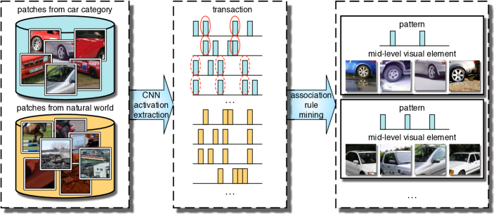
Figure 2: An illustration of the mid-level deep pattern mining process. Given image patches sampled from both the target category (e.g., car) and the background class we represent each as a transaction after extracting their CNN activation. Patterns are then discovered by the well-known association rule mining. Mid-level visual elements are retrieved from image patches with the same patterns.

An overview of the proposed the MDPM algorithm is illustrated in Fig. 2. Assuming that image labels are known, we start by sampling a huge number of random patches both from images of the target category (e.g., car) and images that do not contain the target category (i.e., the background class). With the two appealing properties of CNN activations of image patches (Sec. 4.1), we then create a transaction database in which each transaction corresponds to a particular image patch (Sec. 4.2). Patterns are then discovered from the transaction database using association rule mining (Sec. 4.3), from which mid-level visual elements can be retrieved efficiently (Sec. 4.4).

4.1 Properties of CNN activation of patches

In this section we provide a detailed analysis of the performance of CNN activations on the MIT Indoor dataset [71], from which we are able to deduce two important properties thereof. These two properties are critical to the suitability of such activations to form the basis of a transaction-based approach.

We first sample $128\times 128$ patches with a stride of $32$ pixels from each image. Then, for each image patch, we extract the $4096$-dimensional non-negative output of the first fully-connected layer of BVLC Reference CaffeNet [49]. To generate image features, we consider the following three strategies. The first strategy is our baseline, which is simply the outcome of max pooling on CNN activations of all patches in an image. The next two strategies are variants of the baseline which are detailed as follows.

1. CNN-Sparsified. For each $4096$-dimensional CNN activation of an image patch, we retain the magnitudes of only the $K$ largest elements in the vector, setting the remaining elements to zero. The feature representation for an image is the outcome of applying max pooling to the thus revised CNN activations.

2. CNN-Binarized. For each $4096$-dimensional CNN activation of an image patch, we set the $K$ largest elements in the vector to one and the remaining elements to zero. The feature representation for an image is the outcome of performing max pooling on these binarized CNN activations.

For each strategy we train a multi-class linear SVM classifier in a one-vs-all fashion. The classification accuracy achieved by each of the two above strategies for a range of $K$ values is summarized in Table 1. In comparison, our baseline method gives an accuracy of $65.15$%. Analyzing the results in Table 1 leads to two observations of CNN activations of fully-connected layers (expect the last classification layer):

$K$	$10$	$20$	$50$	$100$
CNN-Sparsified	$50.10$	$56.33$	$60.34$	$61.68$
CNN-Binarized	$54.34$	$59.15$	$61.35$	$61.29$

Table 1: Classification accuracies achieved by the two strategies for keeping the $K$ largest magnitudes of CNN activations of image patches on the MIT Indoor dataset. Note that our baseline, the outcome of max pooling on CNN activations of all patches in an image, gives an accuracy of $65.15$%.

1. Sparse. Comparing the performance of “CNN-Sparsified” with that of the baseline feature ($65.15$%), it is clear that accuracy is reasonably high when using sparsified CNN activations with a small fraction of non-zero magnitudes out of $4096$.

2. Binary. Comparing “CNN-Binarized” with the “CNN-Sparsified” counterpart, it can be seen that CNN activations do not suffer from binarization when $K$ is small. Accuracy even increases slightly in some cases.

Note that the above properties are also observed in recent works on analyzing CNNs [2, 26].

Conclusion. The above two properties imply that for an image patch, the discriminative information within its CNN activation is mostly embedded in the dimension indices of the $K$ largest magnitudes.

4.2 Transaction creation

Transactions must be created before any pattern mining algorithm can proceed. In our work, as we aim to discover patterns from image patches, a transaction is created for each image patch.

The most critical issue now is how to transform an image patch into a transaction while retaining as much information as possible. Fortunately the analysis above (Sec. 4.1) illustrates that CNN activations are particularly well suited to the task. Specifically, we treat each dimension index of a CNN activation as an item ($4096$ items in total). Given the performance of the binarized features shown above, each transaction is then represented by the dimension indices of the $K$ largest elements of the corresponding image patch.

This strategy satisfies both requirements for applying pattern mining techniques (Sec. 3). Specifically, given little performance is lost when using a sparse representation of CNN activations (‘sparse property’ in Sec. 4.1), each transaction calculated as described contains only a small number items ($K$ is small). And because binarization of CNN activations has little deleterious effect on classification performance (‘binary property’ in Sec. 4.1), most of the discriminative information within a CNN activation is retained by treating dimension indices as items.

Following the work of [70], at the end of each transaction, we add a $pos$ (or $neg$) item if the corresponding image patch comes from the target category (or the background class). Therefore, each complete transaction has $K+1$ items, consisting of the indices of the $K$ largest elements in the CNN activation plus one class label. For example, if we set $K=3$, given a CNN activation of an image patch from the target category which has $3$ largest magnitudes in its 3rd, $100$-th and $4096$-th dimensions, the corresponding transaction will be $\{3,100,4096,pos\}$.

In practice, we first sample a large number of patches from images in both the target category and the background class. After extracting their CNN activations, a transaction database $\mathcal{D}$ is created, containing a large number of transactions created using the proposed technique. Note that the class labels, $pos$ and $neg$, are represented by $4097$ and $4098$ respectively in the transactions.

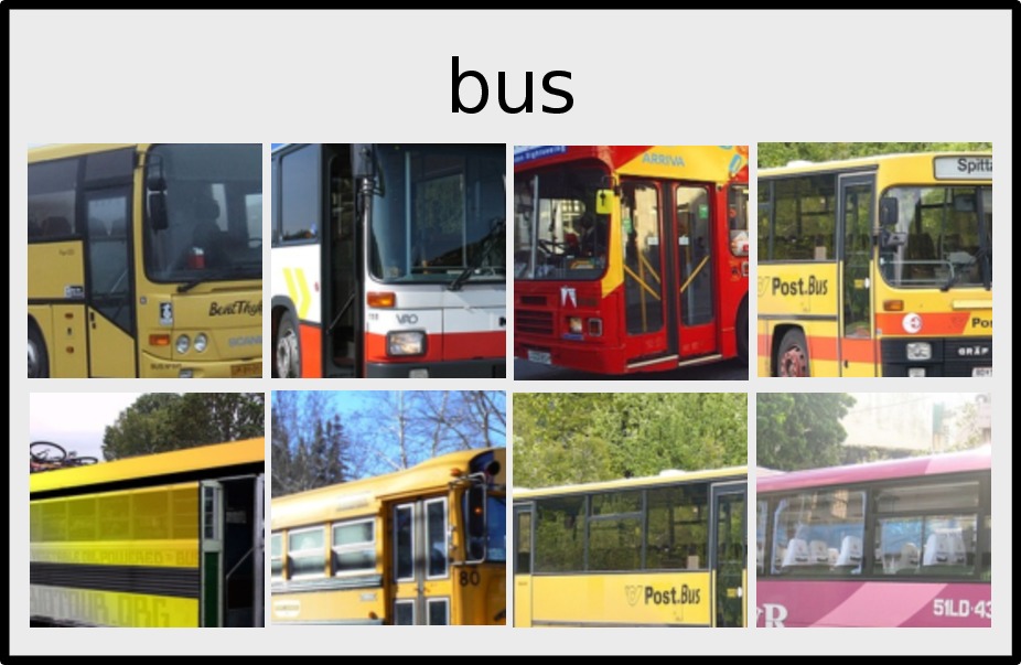
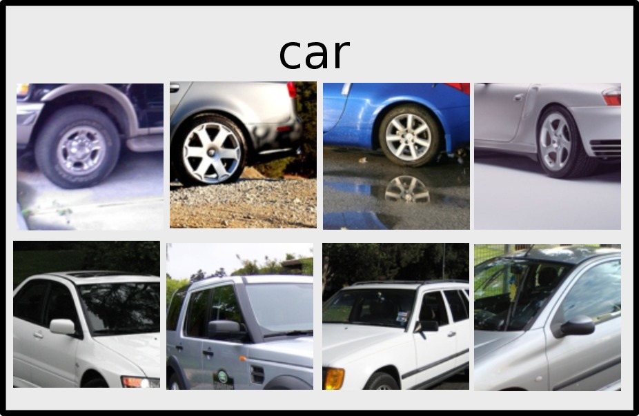
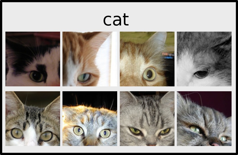
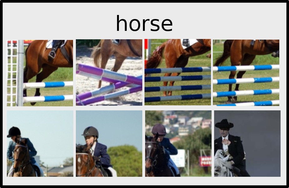
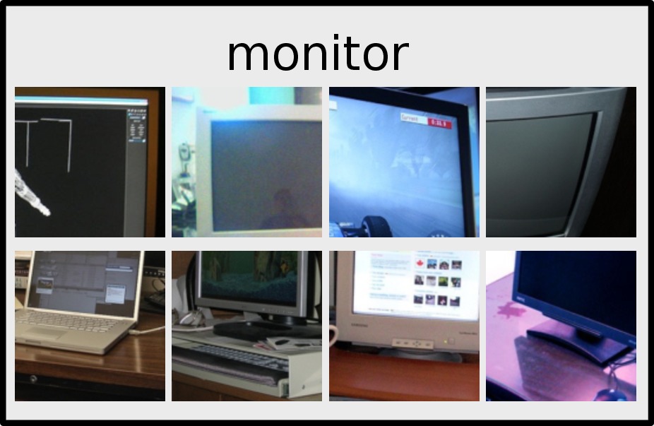
Figure 3: Mid-level visual elements discovered by our algorithm on the Pascal VOC 2007 dataset (for each category, each row is one exemplar).

4.3 Mining representative and discriminative patterns

Given the transaction database $\mathcal{D}$ constructed in Sec. 4.2, we use the Aprior algorithm [3] to discover a set of patterns $\mathcal{P}$ through association rule mining. More specifically, Each pattern $P\in\mathcal{P}$ must satisfy the following two criteria:

$${\mathrm{supp}}(P) >{\mathrm{supp}}_{\min},$$ (3)

$${\mathrm{conf}}(P\rightarrow pos) >{\mathrm{conf}}_{\min},$$ (4)

where ${\mathrm{supp}}_{\min}$ and ${\mathrm{conf}}_{\min}$ are thresholds for the support value and confidence.
Representativeness and discriminativeness. We now demonstrate how association rule mining implicitly satisfies the two requirements of mid-level visual element discovery, i.e., representativeness and discriminativeness. Specifically, based on Eq. (3) and Eq. (4), we are able to rewrite Eq. (2) thus

$$\begin{split}{\mathrm{supp}}(P\cup\{pos\})&={\mathrm{supp}}(P)\times{\mathrm{conf}}(P\rightarrow pos)\\ &>{\mathrm{supp}}_{\min}\times{\mathrm{conf}}_{\min},\end{split}$$ (5)

where ${\mathrm{supp}}(P\cup\{pos\})$ measures the fraction of pattern $P$ found in transactions of the target category among all the transactions. Therefore, having values of ${\mathrm{supp}}(P)$ and ${\mathrm{conf}}(P\rightarrow pos)$ larger than their thresholds ensure that pattern $P$ is found frequently in the target category, akin to the representativeness requirement. A high value of ${\mathrm{conf}}_{\min}$ (Eq. (4)) also ensures that pattern $P$ is more likely to be found in the target category rather than the background class, reflecting the discriminativeness requirement.

4.4 Retrieving mid-level visual elements

Given the set of patterns $\mathcal{P}$ discovered in Sec. 4.3, finding mid-level visual elements is straightforward. A mid-level visual element $V$ contains the image patches sharing the same pattern $P$, which can be retrieved efficiently through an inverted index. This process outputs a set of mid-level visual elements $\mathcal{V}$ (i.e., $V\in\mathcal{V}$).

We provide a visualization of some of the discovered mid-level visual elements in Fig. 3. It is clear that image patches in each visual element are visually similar and depicting the same semantic concept while being discriminative from other categories. For instance, some mid-level visual elements catch discriminative parts of objects (e.g., cat faces found in the cat category), and some depict typical objects or people in a category (e.g., horse-rider found in the horse category). An interesting observation is that mid-level elements discovered by the proposed MDPM algorithm are invariant to horizontal flipping. This is due to the fact that original images and their horizontal flipping counterparts are fed into the CNN during the pre-training process.

5 Image representation

To discover patterns from a dataset containing $Y$ categories, each category is treated as the target category while all remaining $Y-1$ categories in the dataset are treated as the background class. Thus $Y$ sets of patterns will be discovered by the MDPM algorithm, one for each of the $Y$ categories. Given the $Y$ sets of patterns and retrieved mid-level visual elements, we propose two methods to generate image feature representations. The first method is to use a subset of patterns (Sec. 5.1), whereas the second one relies on the retrieved mid-level visual elements (Sec. 5.2). The details of both methods are as follows.

5.1 Encoding an image using patterns

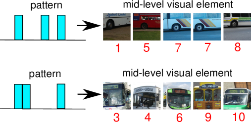
Figure 4: An illustration of the pattern selection process (Sec. 5.1.1). For each pattern on the left, the image patches which form the corresponding mid-level visual elements are shown on the right. The red number underneath each patch is the image index. Since the top and bottom pattern cover $4$ and $5$ unique images, the coverage values of them are $4$ and $5$ respectively.

5.1.1 Pattern selection

Due the problem of pattern explosion (Sec. 3.3), we first select a subset of the discovered patterns based on a simple criterion. We define the coverage of a pattern and its retrieved mid-level visual element as the number of unique images that image patches in this element comes from (see Fig. 4 for an intuitive example). Then, we rank the patterns using the proposed coverage criterion. The intuition here is that we aim to find the patterns whose corresponding mid-level elements cover as many different images as possible, resembling the “Purity-Coverage Plot” in [24]. Thus, from each category, we select $X$ patterns whose corresponding mid-level elements have top-$X$ coverage values. Then, the selected patterns from all $Y$ categories are combined into a new set of patterns $\hat{\mathcal{P}}$ which contains $X\times Y$ elements in total.

5.1.2 Bag-of-Patterns representation

To encode a new image using a set of patterns $\hat{\mathcal{P}}$, we first sample image patches at multiple scales and locations, and extract their CNN activations. For each 4096-dimensional CNN activation vector of an image patch, after finding $C_{i}$, the set of indices of dimensions that have non-zero values, we check for each selected pattern $P_{k}\in\hat{\mathcal{P}}$ whether $P\subseteq C_{i}$. Thus, our Bag-of-Patterns representation (BoP for short) $f_{BoP}\in\mathbf{R}^{X\times Y}$ is a histogram encoding of the set of local CNN activations, satisfying $[f_{BoP}]_{k}=|\{i|P_{k}\in C_{i}\}|$.

Our Bag-of-Patterns representation is similar to the well-known Bag-of-Visual-Words (BoW) representation [81] if one thinks of a pattern $P\in\hat{\mathcal{P}}$ as one visual word. The difference is that in the BoW model one local descriptor is typically assigned to one visual word, whereas in our BoP representation, multiple patterns can fire given on the basis of a CNN activation (and thus image patch). Note that BoP representation has also been utilized by  [34] for image retrieval. In practice, we also add a $2$-level ($1\times 1$ and $2\times 2$) spatial pyramid [52] when computing the BoP representation. More specifically, to generate the final feature representation, we concatenate the normalized BoP representations extracted from different spatial cells.

5.2 Encoding an image using mid-level elements

Due to the redundant nature of the discovered patterns, mid-level visual elements retrieved from those patterns are also likely to be redundant.

For the purpose of removing this redundancy, we merge mid-level elements that are both visually similar and which depict the same visual concept (Sec. 5.2.1). Patch detectors trained from the merged mid-level elements can then be used to construct a Bag-of-Elements representation (Sec. 5.2.2).

Input: A set of partially redundant visual elements $\mathcal{V}$

Output: A set of clean mid-level visual elements $\mathcal{V}^{\prime}$ and corresponding patch detectors $D$

Initialize $\mathcal{V}^{\prime}\leftarrow\emptyset$, $D_{c}\leftarrow\emptyset$;

while $\mathcal{V}\neq\emptyset$ do

       $[\mathcal{V}_{t},d]\leftarrow\textnormal{{MergingTrain}}(\mathcal{V})$;

       $\mathcal{V}\leftarrow\mathcal{V}\setminus\mathcal{V}_{t}$;

       $\mathcal{V}^{\prime}\leftarrow\mathcal{V}^{\prime}\cup\{\mathop{\cup}\limits_{V\in\mathcal{V}_{t}}V\}$;

       $D\leftarrow D\cup\{d\}$;

      

end while

return $\mathcal{V}^{\prime}$, $D$;

Function MergingTrain($\mathcal{V}$)

       Select $V^{\ast}\in\mathcal{V}$ which covers the maximum number of training images;

       Initialize $\mathcal{V}_{t}\leftarrow\{V^{\ast}\}$, $\mathcal{S}\leftarrow\emptyset$ ;

      

      repeat

             $\mathcal{V}_{t}\leftarrow\mathcal{V}_{t}\cup\mathcal{S}$;

             Train LDA detector $d$ using $\mathcal{V}_{t}$;

             $\mathcal{S}\leftarrow\{V\in\mathcal{V}\setminus\mathcal{V}_{t}|\textnormal{{Score}}(V,d)>Th$} where $\textnormal{{Score}}(V,d)=\frac{1}{|V|}\sum_{x\in V}d^{T}x$ ($Th$ is a pre-defined threshold);

            

      until $\mathcal{S}=\emptyset$;

      return $\mathcal{V}_{t}$, $d$;

      

Algorithm 1 Ensemble Merging Pseudocode

5.2.1 Merging mid-level elements

We propose to merge mid-level elements while simultaneously training corresponding detectors using an iterative approach.

Algorithm 1 summarizes the proposed ensemble merging procedure. At each iteration, we greedily merge overlapping mid-level elements and train the corresponding detector through the MergingTrain function in Algorithm 1. In the MergingTrain function, we begin by selecting the element covering the maximum number of training images, and then train a Linear Discriminant Analysis (LDA) detector [44]. The LDA detector has the advantage that it can be computed efficiently using a closed-form solution $\Sigma^{-1}(\bar{x}_{p}-\bar{x})$ where $\bar{x}_{p}$ is the mean of CNN activations of positive samples, $\bar{x}$ and $\Sigma$ are the mean and covariance matrix respectively which are estimated from a large set of random CNN activations. Inspired by previous works [50, 53, 80], We then incrementally revise this detector. At each step, we run the current detector on the activations of all the remaining mid-level elements, and retrain it by augmenting the positive training set with positive detections. We repeat this iterative procedure until no more elements can be added into the positive training set. The idea behind this process is using the detection score as a similarity metric, inspired by Exemplar SVM [61, 77]. The output of the ensemble merging step is a merged set of mid-level elements and their corresponding detectors. The limitation of the proposed merging method is that the merging threshold $Th$ (see Algorithm 1) needs to be tuned, which will be analyzed in the experiment (Sec. 6.2.1).

After merging mid-level elements, we again use the coverage criterion (Sec. 5.1.1) to select $X$ detectors of merged mid-level elements for each of the $Y$ categories and stack them together.

5.2.2 Bag-of-Elements representation

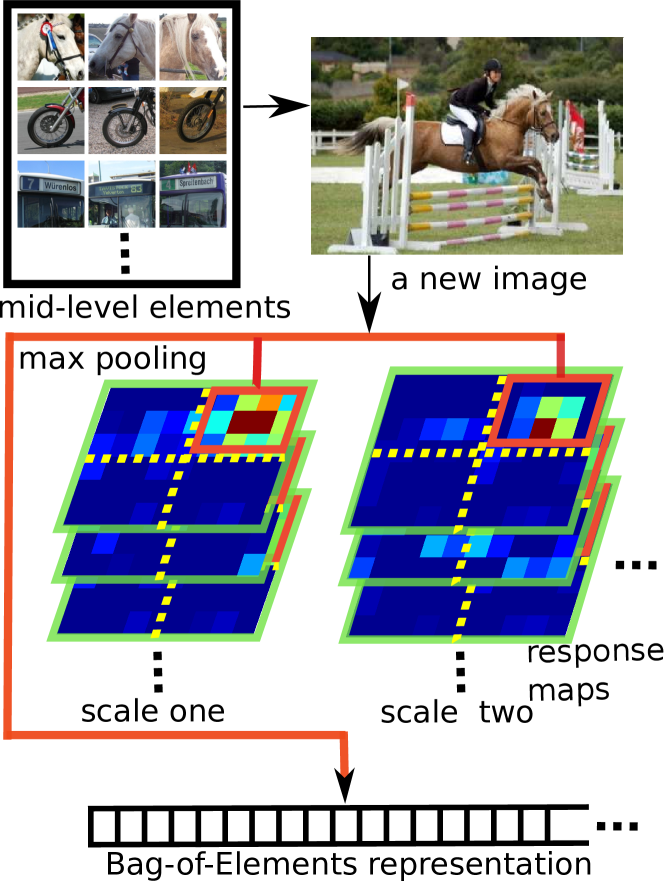
Figure 5: Pipeline to construct a Bag-of-Elements representation, which has been used in previous works as well [80, 24, 50, 7].

As shown in previous works on mid-level visual element discovery [80, 50, 24, 7], detectors of mid-level elements can be utilized to generate a Bag-of-Elements representation. An illustration of this process is shown in Fig. 5. Concretely, given an image, we evaluate each of the detectors at multiple scales, which results in a stack of response maps of detection scores. For each scale, we take the max score per detector per region encoded in a $2$-level ($1\times 1$ and $2\times 2$) spatial pyramid. The final feature representation of an image has $X\times Y\times 5$ dimensions, which is the outcome of max pooling on the responses from all scales in each spatial cell.

6 Experiments

This section contains an extensive set of experimental result and summarizes the main findings. Firstly, some general experimental setups (e.g., datasets, implementation details) are discussed in Sec. 6.1, followed by detailed analysis of the proposed approach on object (Sec. 6.2) and indoor scene (Sec. 6.3) classification tasks respectively. Rely on the discovered mid-level visual elements. Sec. 6.4 provides further analysis of the importance of context information for recognition, which seldom appears in previous works on mid-level elements.

6.1 Experimental setup

6.1.1 CNN models

For extracting CNN activations from image patches, we consider two state-of-the-art CNN models which are both pre-trained on the ImageNet dataset [21]. The first CNN model is the BVLC Reference CaffeNet [49] (CaffeRef for short), whose architecture is similar to that of AlexNet [51], that is, five convolution layers followed by two 4096-dimensional and one 1000-dimensional fully-connected layers. The second CNN model is the 19-layer VGG-VD model [79] which has shown good performance in the ILSVRC-2014 competition [75]. For both models, we extract the non-negative 4096-dimensional activation from the first fully-connected layer after the rectified linear unit (ReLU) transformation as image patch representations.

6.1.2 Datasets

We evaluate our approach on three publicly available image classification datasets, two for generic object classification and the other for scene classification. The details of the datasets are as follows.

Pascal VOC 2007 dataset. The Pascal VOC 2007 dataset [29, 28] contains a total of $9,963$ images from $20$ object classes, including $5,011$ images for training and validation, and $4,952$ for testing. For evaluating different algorithms, mean average precision (mAP) is adopted as the standard quantitative measurement.

Pascal VOC 2012 dataset. The Pascal VOC 2012 dataset [29, 28] is an extension of the VOC 2007 dataset, which contains a total of $22,531$ images from $20$ object classes, including $11,540$ images for training and validation, and $10,991$ for testing. We use the online evaluation server of this dataset to evaluate the proposed approach.

MIT Indoor dataset. The MIT Indoor dataset [71] contains 67 classes of indoors scenes. A characteristic of indoor scenes is that unique configurations or objects are often found in a particular scene, e.g., computers are more likely to be found in a computer room rather than a laundry. For this reason, many mid-level element discovery algorithms [80, 50, 24, 83, 9] are evaluated on this dataset and have achieved state-of-the-art performance. We follow the standard partition of [71], i.e., approximately 80 training and 20 test images per class. The evaluation metric for MIT Indoor dataset is the mean classification accuracy.

6.1.3 Implementation details

Given an image, we resize its smaller dimension to $256$ while maintaining its aspect ratio, then we sample $128\times 128$ patches with a stride of $32$ pixels, and calculate the CNN activations from Caffe (using either the CaffeRef or VGG-VD models). When mining mid-level visual elements, only training images are used to create transactions (trainval set for Pascal VOC datasets). The length of each is transaction is set as $20$, which corresponds to $20$ largest dimension indices of CNN activations of an image patch. We use the implementation of association rule mining from [8]. The merging threshold $Th$ in Algorithm 1 (Sec. 5.2.1) is set as $150$. For generating image features for classification, CNN activations are extracted from five scales for the Pascal VOC datasets as compared to three scales for the MIT Indoor dataset (we experimentally found using more than three scales for MIT Indoor does not improve the overall classification performance. ) . For training image classifiers, we use the Liblinear toolbox [30] with $5$-fold cross validation. For association rule mining, the value of $supo_{min}$ (Eq. 3) is always set as $0.01$% whereas the value of $conf_{min}$ (Eq. 4) is tuned for different datasets.

6.2 Object classification

In this section, we provide a detailed analysis of the proposed system for object classification on the Pascal VOC 2007 and 2012 datasets. We begin with an ablation study which illustrates the importance of the different components of our system (Sec. 6.2.1). In Sec. 6.2.2, we compare our system with state-of-the-art algorithms which also rely on CNNs, followed by computational complexity analysis in Sec. 6.2.4. Some visualizations of mid-level visual elements are provided in Sec. 6.2.3. On VOC 2007 dataset, the ${\mathrm{conf}}_{\min}$ (Eq. 4) is set as $60\%$ for CaffRef and $80\%$ for VGG-VD model respectively. On VOC 2012 dataset, we use $40\%$ for ${\mathrm{conf}}_{\min}$ when VGG-VD model is adopted.

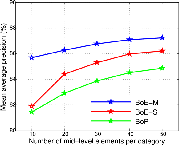
(a)

(b)

Figure 6: Performance of proposed feature encoding methods on the Pascal VOC 2007 dataset. Note that VGG-VD model is used for evaluation.

6.2.1 Ablation study

Bag-of-Elements vs. Bag-of-Patterns. We analyze the performance achieved by different encoding methods proposed in Sec. 5. We denote the the Bag-of-Patterns representation as BoP, and the Bag-of-Elements representation constructed after the merging process as BoE-M. We also implement another encoding method, BoE-S which does not merge mid-level elements but rather select mid-level elements from a large pool of candidates using the coverage criterion. The performance of the above encoding methods are illustrated in Fig. 6.

As is illustrated in Fig. 6, when using the same number of mid-level elements and the same CNN model, the Bag-of-Elements representation significantly outperforms the Bag-of-Patterns representation. This could be interpreted as resulting from the “hard-assignment” process at the heart of the Bag-of-Patterns method. In contrast, Bag-of-Elements does not suffer from this problem because it relies on the detection responses of the patch detectors. Compared with direct selection of mid-level elements, performance is consistently boosted when mid-level elements are first merged (BoE-M vs. BoE-S), which shows the importance of the proposed merging algorithm (c.f. Algorithm 1). Therefore, we use our best encoding method, BoE-M, to compare with the state-of-the-art below (note that the suffix is dropped).

Number of mid-level elements. Irrespective of the CNN architecture or encoding method, adding more mid-level elements or patterns to construct image features consistently improves classification accuracy (see Fig. 6). Note also that the performance gain is large when a small number of mid-level elements (patterns) are used (e.g., from $10$ to $20$), and seems to saturate when the number of mid-level elements reaches $50$. This is particularly interesting given the differences between the datasets and the CNN networks used.

Transaction length. We evaluate the performance of our approach under three settings of the transaction length, which are $10$, $20$ and $30$ respectively. Table 2 depicts the results. It is clear from Table 2 that more information will be lost when using a smaller transaction length. However, as the search space of the association rule mining algorithm grows exponentially with the transaction length, this value cannot be set very large or otherwise it becomes both time and memory consuming. Therefore, we opt for $20$ as the default setting for transaction length as a tradeoff between performance and time efficiency.

transaction length	$10$	$20$	$30$
mAP ($\%$)	$85.4$	$87.3$	$87.6$

Table 2: Analysis of the transaction length on the VOC 2007 dataset using the VGG-VD model. Other parameters are frozen.

$Th$	$50$	$100$	$150$	$200$
mAP ($\%$)	$86.4$	$87.2$	$87.3$	$87.0$

Table 3: Analysis of the merging threshold $Th$ in Algorithm 1 on the VOC 2007 dataset using the VGG-VD model. Other parameters are frozen.

VOC 2007 test	aero	bike	bird	boat	bottle	bus	car	cat	chair	cow	table	dog	horse	mbike	person	plant	sheep	sofa	train	tv	mAP
FC (CaffeRef)	$87.2$	$78.1$	$79.4$	$79.3$	$25.4$	$63.3$	$81.2$	$75.0$	$46.6$	$53.7$	$61.8$	$65.1$	$82.8$	$70.7$	$88.5$	$39.4$	$69.2$	$51.1$	$87.5$	$60.0$	$67.3$
FC (VGG-VD)	$95.2$	$85.5$	$89.9$	$88.1$	$45.9$	$81.7$	$89.3$	$88.6$	$55.2$	$73.2$	$75.1$	$84.3$	$91.3$	$87.0$	$92.2$	$48.4$	$80.1$	$70.9$	$95.2$	$74.1$	$79.6$
[73]	$88.5$	$81.0$	$83.5$	$82.0$	$42.0$	$72.5$	$85.3$	$81.6$	$59.9$	$58.5$	$66.5$	$77.8$	$81.8$	$78.8$	$90.2$	$54.8$	$71.1$	$62.6$	$87.4$	$71.8$	$73.9$
[58]	$89.5$	$84.1$	$83.7$	$83.7$	$43.9$	$76.7$	$87.8$	$82.5$	$60.6$	$69.6$	$72.0$	$77.1$	$88.7$	$82.1$	$94.4$	$56.8$	$71.4$	$67.7$	$90.9$	$75.0$	$76.9$
[14]	$95.3$	$90.4$	$92.5$	$89.6$	$54.4$	$81.9$	$91.5$	$91.9$	$64.1$	$76.3$	$74.9$	$89.7$	$92.2$	$86.9$	$95.2$	$60.7$	$82.9$	$68.0$	$95.5$	$74.4$	$82.4$
[64]	$88.5$	$81.5$	$87.9$	$82.0$	$47.5$	$75.5$	$90.1$	$87.2$	$61.6$	$75.7$	$67.3$	$85.5$	$83.5$	$80.0$	$95.6$	$60.8$	$76.8$	$58.0$	$90.4$	$77.9$	$77.7$
[45]	$91.9$	$88.6$	$91.2$	$89.5$	$63.0$	$81.8$	$88.7$	$90.1$	$62.7$	$79.6$	$72.8$	$88.7$	$90.0$	$85.8$	$93.5$	$63.8$	$88.4$	$68.1$	$92.1$	$78.7$	$82.4$
[94]	$95.1$	$90.1$	$92.8$	$89.9$	$51.5$	$80.0$	$91.7$	$91.6$	$57.7$	$77.8$	$70.9$	$89.3$	$89.3$	$85.2$	$93.0$	$64.0$	$85.7$	$62.7$	$94.4$	$78.3$	$81.5$
[90]	$96.7$	$83.1$	$94.2$	$92.8$	$61.2$	$82.1$	$89.1$	$94.2$	$64.2$	$83.6$	$70.0$	$92.4$	$91.7$	$84.2$	$93.7$	$59.8$	$93.2$	$75.3$	$99.7$	$78.6$	$84.0$
[17]	$91.3$	$90.5$	$91.3$	$88.9$	$66.4$	$85.6$	$91.1$	$90.7$	$71.3$	$79.8$	$82.8$	$90.1$	$90.8$	$88.6$	$94.7$	$67.7$	$83.5$	$78.6$	$92.9$	$82.2$	$84.9$
[79]	-	-	-	-	-	-	-	-	-	-	-	-	-	-	-	-	-	-	-	-	$89.3$
BoE (CaffeRef,50)	$90.3$	$85.4$	$82.9$	$79.8$	$45.9$	$75.5$	$89.6$	$85.1$	$61.6$	$60.0$	$71.2$	$79.9$	$88.9$	$83.4$	$94.2$	$53.3$	$65.9$	$67.2$	$91.4$	$76.0$	$76.4$
BoE (VGG-VD,50)	$97.2$	$93.3$	$95.0$	$91.3$	$63.3$	$88.2$	$93.0$	$94.1$	$70.5$	$79.9$	$85.6$	$93.2$	$94.4$	$90.4$	$95.4$	$70.1$	$87.7$	$78.3$	$97.2$	$87.0$	$87.3$

Table 4: Comparison of classification results on the Pascal VOC 2007 dataset. For the sake of fair comparison, CNN models of all above methods are trained using the dataset used in the ILSVRC competition [75], i.e., 1000 classes from the ImageNet [21].

VOC 2012 test	aero	bike	bird	boat	bottle	bus	car	cat	chair	cow	table	dog	horse	mbike	person	plant	sheep	sofa	train	tv	mAP
FC (VGG-VD)	$97.0$	$76.3$	$86.8$	$85.8$	$47.9$	$87.9$	$72.8$	$90.0$	$57.1$	$70.2$	$67.5$	$87.1$	$86.3$	$85.1$	$89.7$	$40.0$	$77.7$	$54.0$	$94.1$	$75.3$	$76.4$
[64]	$93.5$	$78.4$	$87.7$	$80.9$	$57.3$	$85.0$	$81.6$	$89.4$	$66.9$	$73.8$	$62.0$	$89.5$	$83.2$	$87.6$	$95.8$	$61.4$	$79.0$	$54.3$	$88.0$	$78.3$	$78.7$
[98]	$96.0$	$77.1$	$88.4$	$85.5$	$55.8$	$85.8$	$78.6$	$91.2$	$65.0$	$74.4$	$67.7$	$87.8$	$86.0$	$85.1$	$90.9$	$52.2$	$83.6$	$61.1$	$91.8$	$76.1$	$79.0$
[94]	$97.7$	$83.0$	$93.2$	$87.2$	$59.6$	$88.2$	$81.9$	$94.7$	$66.9$	$81.6$	$68.0$	$93.0$	$88.2$	$87.7$	$92.7$	$59.0$	$85.1$	$55.4$	$93.0$	$77.2$	$81.7$
[14]	$96.8$	$82.5$	$91.5$	$88.1$	$62.1$	$88.3$	$81.9$	$94.8$	$70.3$	$80.2$	$76.2$	$92.9$	$90.3$	$89.3$	$95.2$	$57.4$	$83.6$	$66.4$	$93.5$	$81.9$	$83.2$
[79]	-	-	-	-	-	-	-	-	-	-	-	-	-	-	-	-	-	-	-	-	$89.0$
BoE (VGG-VD,50)	$97.9$	$86.3$	$92.2$	$88.6$	$66.2$	$90.4$	$83.6$	$95.2$	$76.6$	$84.1$	$77.3$	$94.9$	$94.6$	$92.5$	$95.5$	$57.5$	$87.3$	$67.9$	$94.6$	$86.3$	$85.5$

Table 5: Comparison of classification results on the Pascal VOC 2012 dataset. For the sake of fair comparison, CNN models of all above methods are trained using the dataset used in the ILSVRC competition [75], i.e., 1000 classes from the ImageNet [21].

The merging threshold. The merging threshold $Th$ in Algorithm 1 controls how many mid-level elements should be merged together. While keeping other parameters fixed, we evaluate this parameter under different settings. As shown in Table 3, the best performance is reached when using value of $150$ for $Th$.

Pattern selection method in [74]. To show the effectiveness of the proposed pattern selection (Sec. 5.1.1) and merging (Sec. 5.2.1) methods, we re-implemented the pattern selection method proposed by [74] and combine it with our framework. In [74], patterns are first ranked according to an interesting score and then non-overlapping patterns are selected in a greedy fashion (please refer to Algorithm 1 in [74]). In our case, after selecting patterns following  [74], we train detectors for the mid-level elements retrieved from those patterns and construct a Bag-of-Elements representation (Sec. 5.2.2). On the VOC 2007 dataset, when using the VGG-VD model and $50$ elements per category, this framework gives $85.0\%$ mAP, which is lower than that of our pattern selection method ($86.2\%$) and pattern merging method ($87.3\%$).

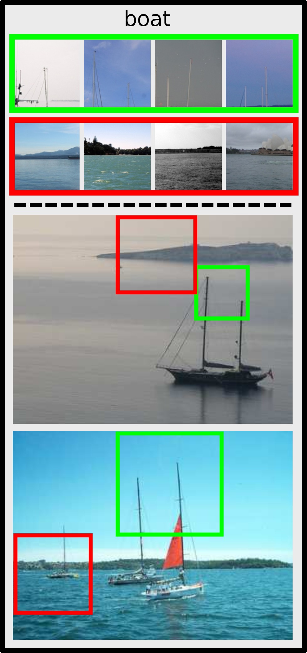
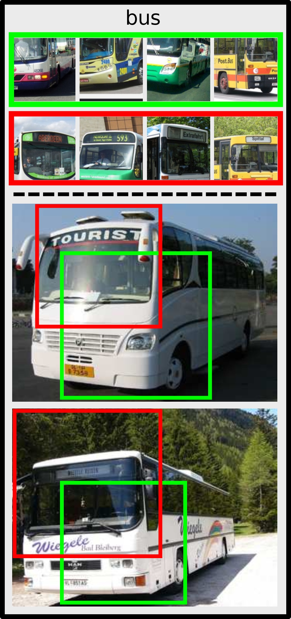
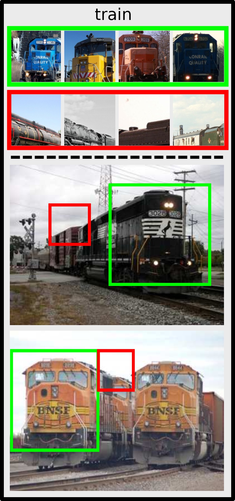
Figure 7: Discovered mid-level visual elements and their corresponding detections on test images on the Pascal VOC 2007 dataset.

6.2.2 Comparison with state-of-the-arts

To compare with the state-of-the-art we use the BoE representation with $50$ mid-level elements per category, which demonstrated the best performance in the ablation study (Fig. 6). We also consider one baseline method (denoted as ‘FC’) in which a 4096-dimensional fully-connected activation extracted from a global image is used as the feature representation. Table 4 summarizes the performance of our approach as well as state-of-the-art approaches on Pascal VOC 2007.

For encoding high-dimensional local descriptors, [58] propose a new variant of Fisher vector encoding [68]. When the same CaffeRef model is used in both methods, our performance is on par with that of [58] ($76.4$% vs. $76.9$%) whereas the feature dimension is $40$ times lower ($5$k vs. $200$k).  [64] adds two more layers on the top of fully-connected layers of the AlexNet and fine-tunes the pre-trained network on the PASCAL VOC. Although the method performs well ($77.7$%), it relies on bounding box annotations which makes the task easier. The FV-CNN method of [18] extracts dense CNN activations from the last convolutional layer and encodes them using the classic Fisher vector encoding. Using the same VGG-VD model, our BoE representation performs better than this method by a noticeable margin ($87.3$% vs. $84.9\%$, despite the fact that we only use half of the image scales of FV-CNN ($5$ vs. $10$) and feature dimension is significantly lower ($5$k vs. $65$k).

As for the VOC 2012 dataset, as shown in Table 5, when using the VGG-VD CNN model and $50$ elements per category, the proposed BoE representation reaches a mAP of $85.5$%, outperforming most state-of-the-art methods.

6.2.3 Visualizing mid-level visual elements

We visualize some mid-level elements discovered by the proposed MDPM algorithm and their firings on test images of the VOC 2007 dataset in Fig. 7.

Clearly, some mid-level visual elements capture discriminative parts of an object (e.g., horse faces for the horse class, the front of locomotives for the train class and wheels for the motorbike class). It is worth noting here these discriminative parts have been shown to be extremely important for state-of-the-art object recognition systems, such as Deformable Part Models [31] and Poselets [12]. Moreover, rather than firing on the underlying object, some mid-level elements focus on valuable contextual information. For instance, as shown in Fig. 7, ‘people’ is an important cue both for the horse and motorbike classes, and ‘coastline’ is crucial for classifying boat. This fact indicates that mid-level elements may be a good tool for analysing the importance of context for image classification (Sec. 6.4).

6.2.4 Computational complexity

The effectiveness of any mid-level visual element discovery process depends on being able to process very large numbers of image patches. The recent work of [67], for example, takes $5$ days to find mid-level elements on the MIT Indoor dataset. The proposed MDPM algorithm has been designed from the beginning with speed in mind, as it is based on a very efficient pattern mining algorithm. Thus, for approximately $0.2$ million transactions created from CNN activations of image patches on the Pascal VOC 2007 dataset, association rule mining takes only $23$ seconds to discover representative and discriminative patterns. The bottleneck of our approach thus lies in the process of extracting CNN activations from image patches, which is slower than the calculation of hand-crafted HOG features. All CNN-based approaches will suffer this time penalty, of course. However, the process can be sped up using the technique proposed in [96] which avoids duplicated convolution operations between overlapping image patches. GPUs can also be used to accelerate CNN feature extraction.

6.3 Scene classification

We now provide detailed analysis of the proposed system for the task of scene classification on the MIT Indoor dataset. As many mid-level element discovery algorithms have reported performance on this dataset, we first provide a comprehensive comparison between these algorithms and our method in Sec. 6.3.1. The comparison between the performance of state-of-the-art methods with CNN involved and ours are presented in Sec. 6.3.2. Finally, we visualize some mid-level elements discovered by the proposed MDPM algorithm and their firings in Sec. 6.3.3. For this dataset, the value of $conf_{min}$ (Eq. 4) is always set as $30\%$.

6.3.1 Comparison with methods using mid-level elements

Method	$\#$ of elements	Acc (%)
[80]	$210$	$38.10$
[50]	$50$	$46.10$
[54]	$20$	$46.40$
[92]	$11$	$50.15$
[83]	$73$	$51.40$
[9]	$50$	$54.40$
[24]	$200$	$64.03$
[67]	$5$	$73.30$
LDA-Retrained (CaffeRef)	$20$	$58.78$
LDA-Retrained (CaffeRef)	$50$	$62.30$
LDA-KNN (CaffeRef)	$20$	$59.14$
LDA-KNN (CaffeRef)	$20$	$63.93$
BoE (CaffeRef)	$20$	$68.24$
BoE (CaffeRef)	$50$	$69.69$
BoE (VGG-VD)	$20$	$76.93$
BoE (VGG-VD)	$50$	$77.63$

Table 6: Classification results of mid-level visual element discovery algorithms on MIT Indoor dataset.

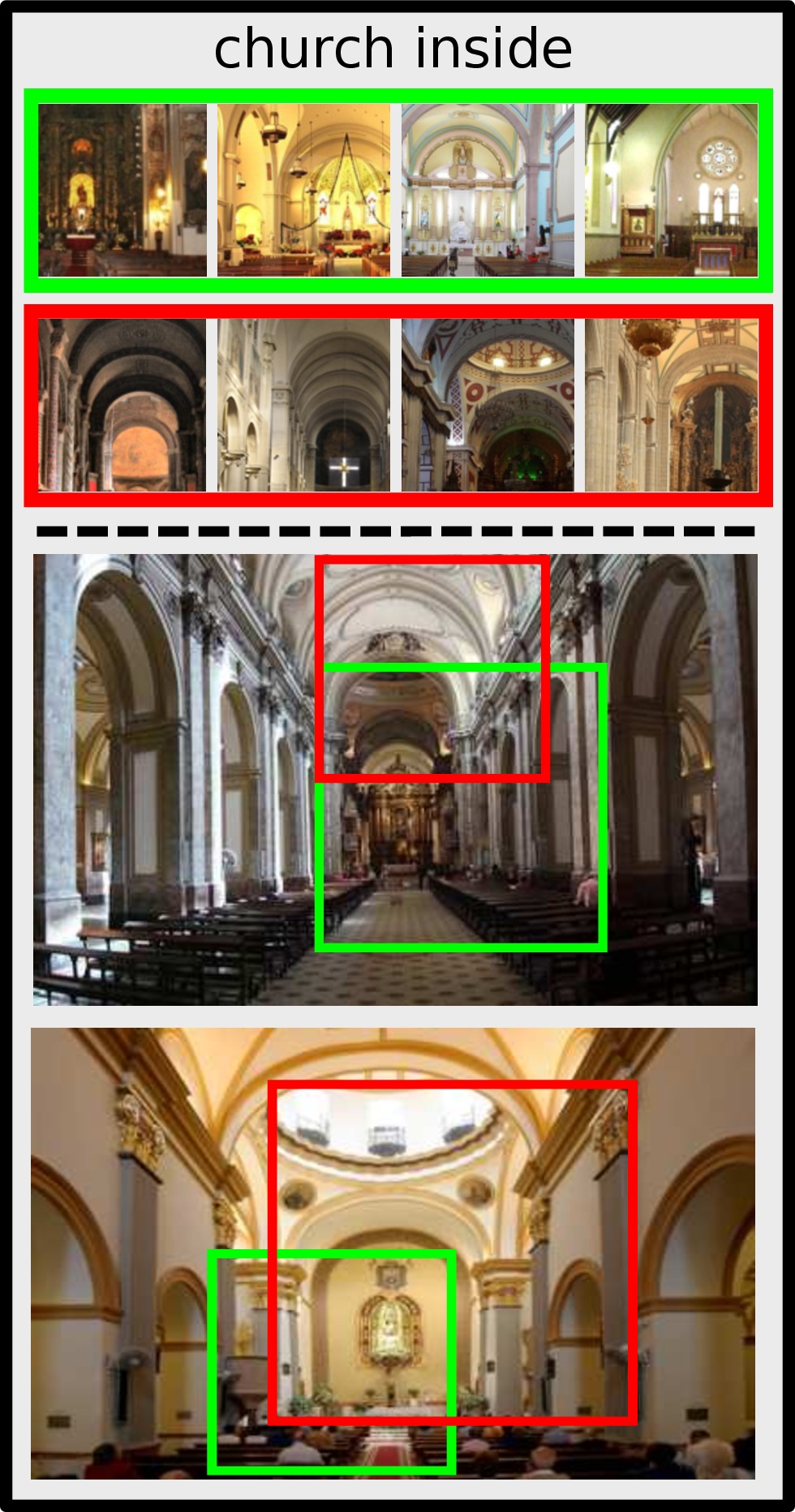
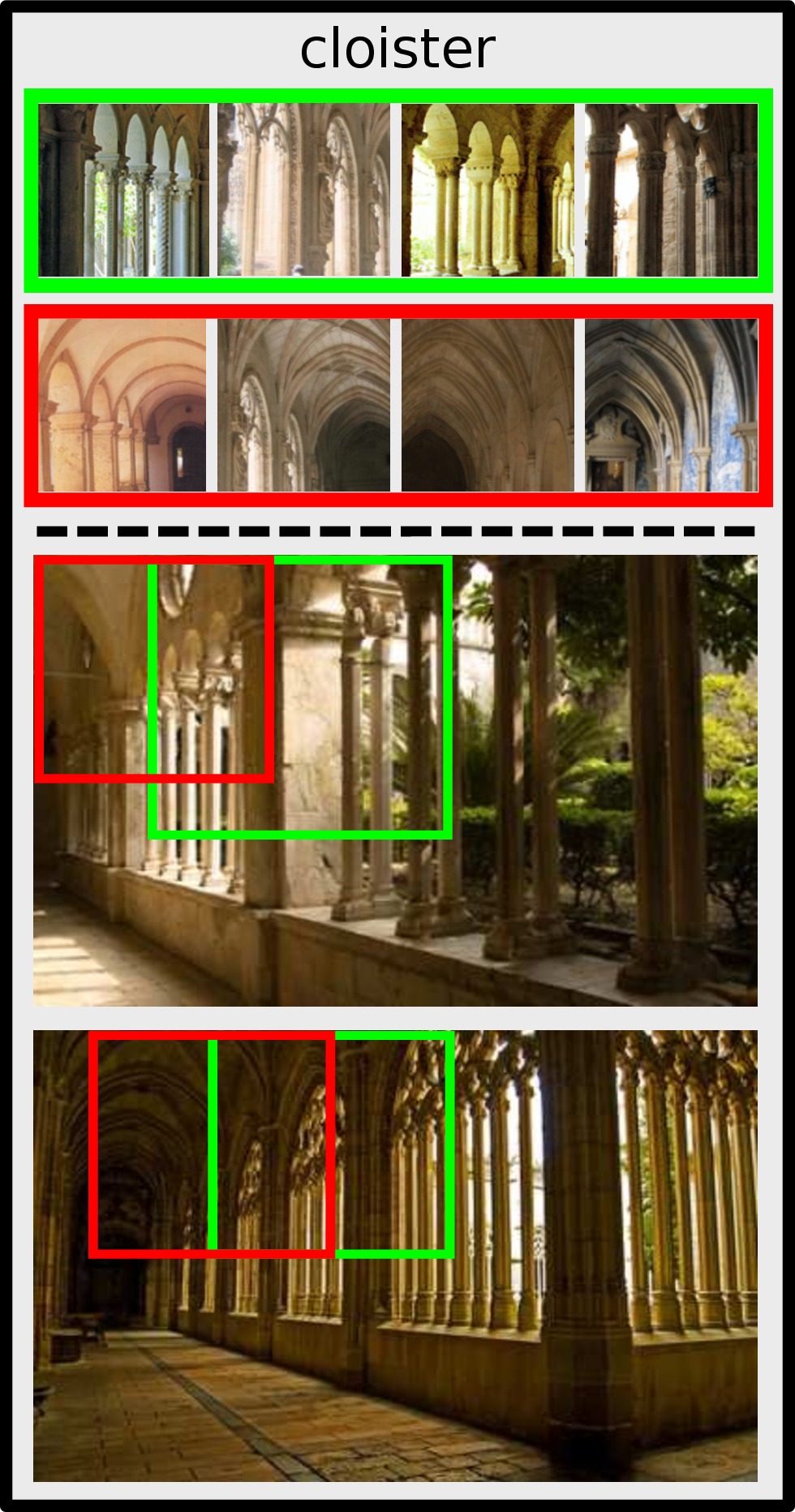
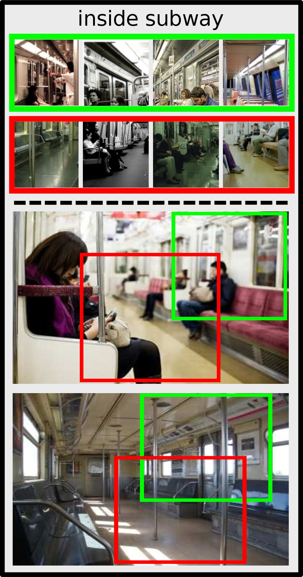
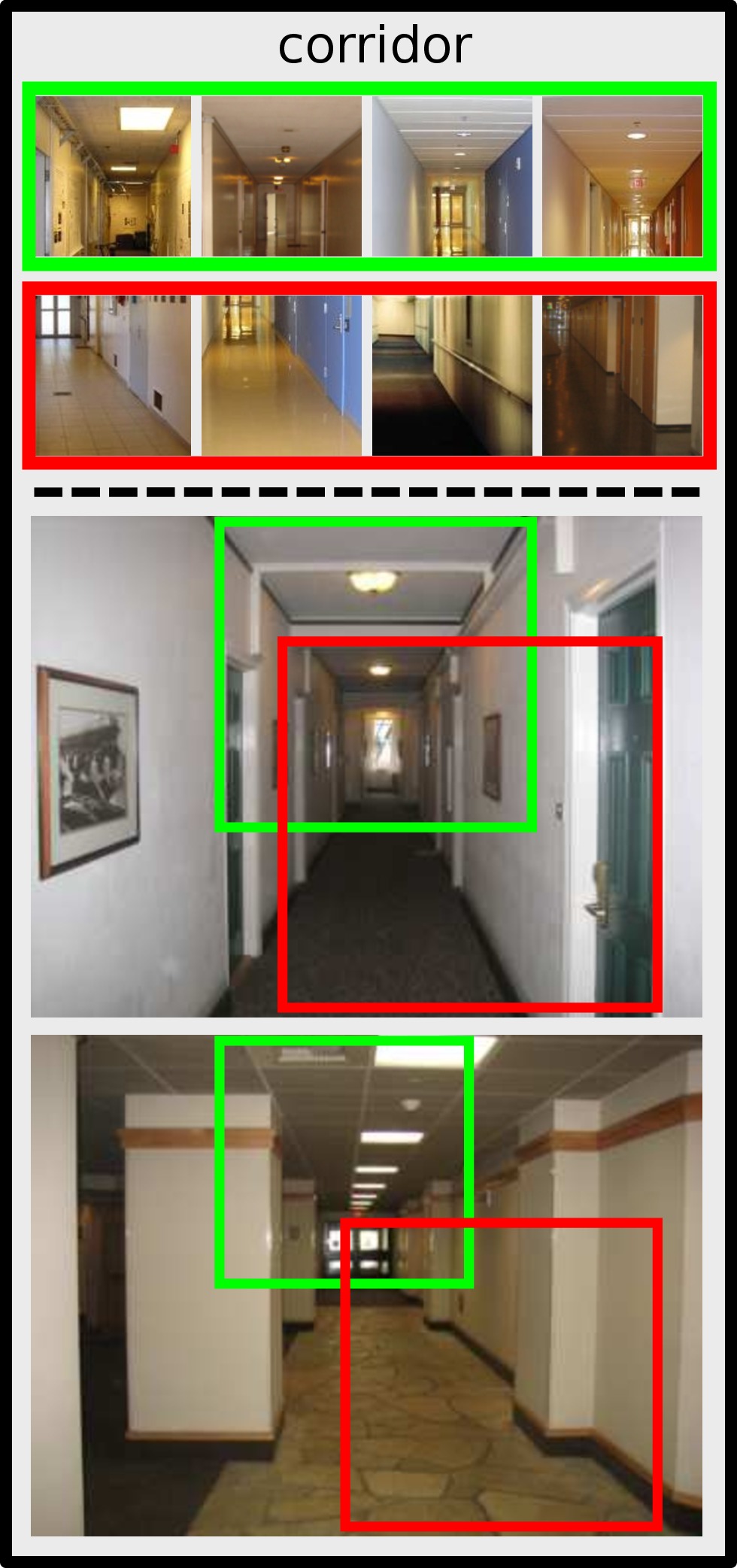
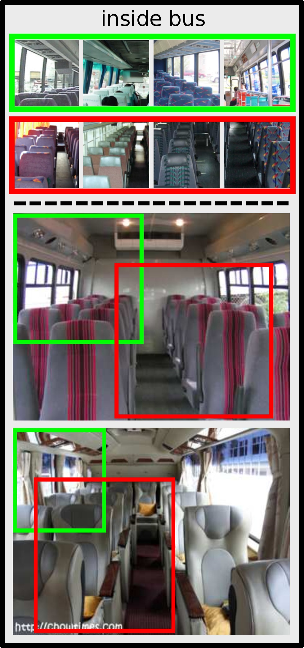
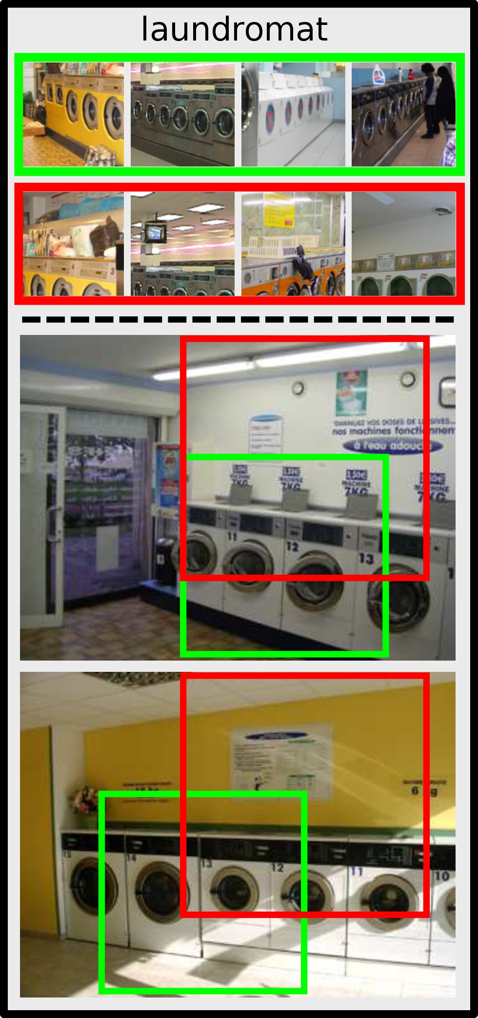
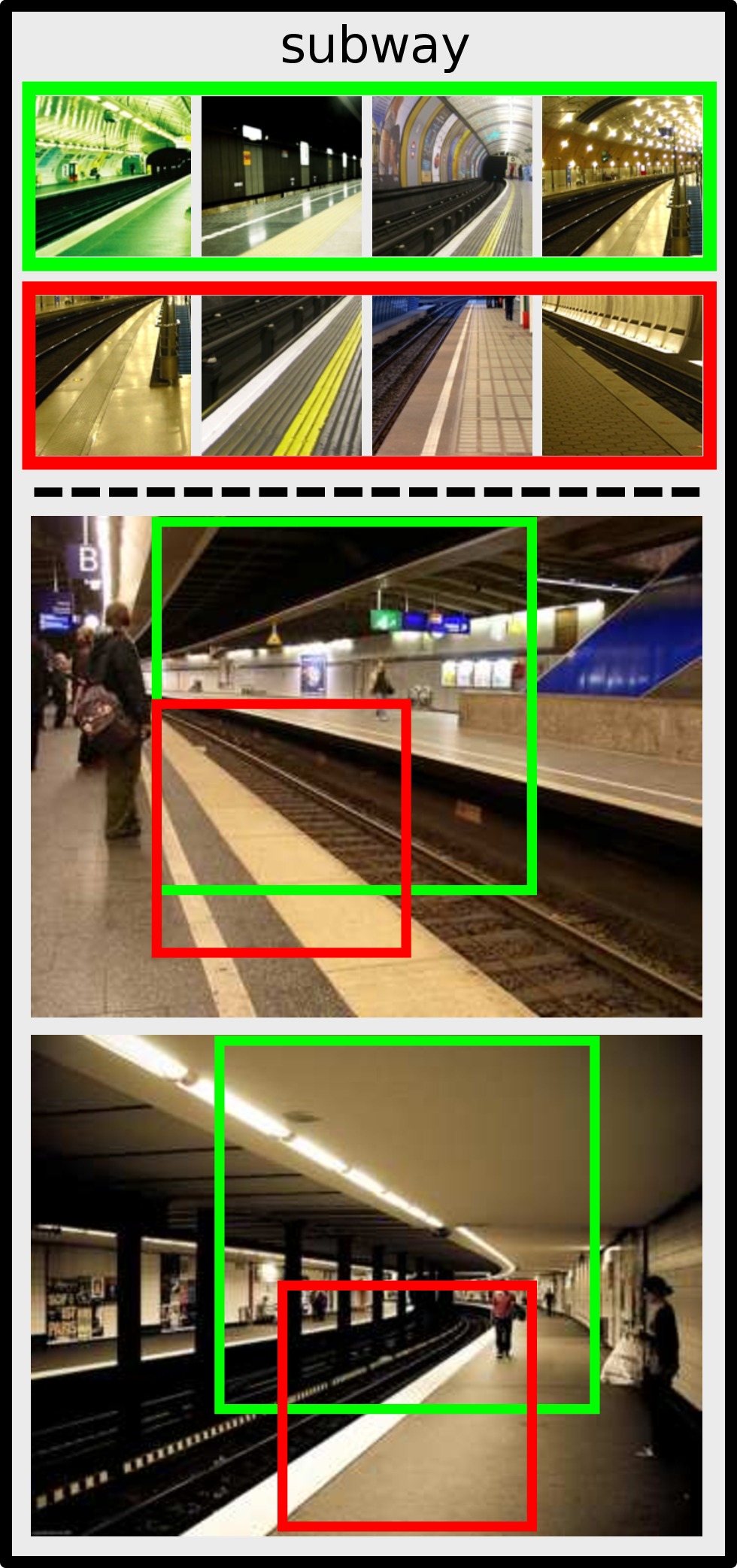
Figure 8: Discovered mid-level visual elements and their corresponding detections on test images on the MIT Indoor dataset.

As hand-crafted features, especially HOG, are widely utilized as image patch representations in previous works, we here analyze the performance of previous approaches if CNN activations are used in place of their original feature types. We have thus designed two baseline methods so as to use CNN activations as an image patch representation.

The first baseline “LDA-Retrained” initially trains Exemplar LDA using the CNN activation of a sampled patch and then re-trains the detector $10$ times by adding top-$10$ positive detections as positive training samples at each iteration. This is similar to the “Expansion” step of [50]. The second baseline “LDA-KNN” retrieves 5-nearest neighbors of an image patch and trains an LDA detector using the CNN activations of retrieved patches (including itself) as positive training data. For both baselines, discriminative detectors are selected based on the Entropy-Rank Curves proposed by [50].

As shown in Table 6, when using the CaffeRef model, MDPM achieves significantly better results than both baselines in the same setting. This attests to the fact that the pattern mining approach at the core of MDPM is an important factor in its performance.

We also compare the proposed method against recent work in mid-level visual element discovery in Table 6. Clearly, by combining the power of deep features and pattern mining techniques, the proposed method outperforms all previous mid-level element discovery methods by a sizeable margin.

6.3.2 Comparison with methods using CNN

Method	Acc (%)	Comments
FC (CaffeRef)	$57.74$	CNN for whole image
FC (VGG-VD)	$68.87$	CNN for whole image
[73]	$58.40$	OverFeat toolbox
[42] (CaffeRef)	$68.88$	concatenation
[6]	$65.90$	jittered CNN
[6]	$66.30$	FT CNN
[100]	$68.24$	Places dataset used
[58] (CaffeRef)	$68.20$	new Fisher encoding
[57] (CaffeRef)	$68.80$	cross-layer pooling
[67]	$73.30$	unified pipeline
[56] (VGG-VD)	$77.55$	Bilinear CNN
[37] (VGG-VD)	$76.17$	compact Bilinear CNN
[63]	$77.40$	shared parts
[17] (VGG-VD)	$81.00$	Fisher Vector
BoE (CaffeRef)	$69.69$	$50$ elements
BoE (VGG-VD)	$77.63$	$50$ elements

Table 7: Classification results of methods using CNN activations on MIT Indoor dataset.

In Table 7, we compare the proposed method to others in which CNN activations are used, at the task of scene classification. The baseline method, using fully-connected CNN activations extracted from the whole image using CaffeRef (resp. VGG-VD), gives an accuracy of $57.74\%$ (resp. $68.87$%). The proposed method achieves $69.69\%$ using CaffeRef and $77.63$% using VGG-VD, which are significant improvements over the corresponding baselines.

Our method is closely related to [42] and  [57] in the sense that all rely on off-the-shelf CNN activations of image patches. Our BoE representation, which is based on mid-level elements discovered by the MDPM algorithm, not only outperforms [42] on $128\times 128$ and $64\times 64$ patches by a considerable margin ($69.69\%$ vs. $65.52\%$ and $69.69\%$ vs. $62.24\%$), it also slightly outperforms that of [57] ($69.69\%$ vs. $68.20\%$). Our performance ($77.63\%$) is also comparable to that of the recent works of bilinear CNN [56] ($77.55\%$) and its compact version [37] ($76.17\%$) when the VGG-VD model is adopted.

Fine-tuning has been shown to be beneficial when transferring pre-trained CNN models to another dataset [40, 64, 2]. We are interested in how the performance changes if a fine-tuned CNN model is adopted in our framework. For this purpose, we first fine-tuned the VGG-VD model on the MIT Indoor dataset with a learning rate of $0.0005$. The fine-tuned model reaches $69.85\%$ accuracy after $70k$ iterations. After applying the fine-tuned model in our framework, the proposed approach reaches $71.82\%$ accuracy, which is lower than the case of using a pre-trained model ($77.63\%$) but still improves the accuracy of directly fine-tuning ($69.85\%$). The underlying reason is probably due to the small training data size of the MIT Indoor dataset and the large capacity of the VGG-VD model. We plan to investigate this issue in our future work. Similar observation was made in [37].

6.3.3 Visualizing mid-level visual elements

We visualize some visual elements discovered and their firings on test images of the MIT Indoor dataset in Fig. 8. It is intuitive that the discovered mid-level visual elements capture the visual patterns which are often repeated within a scene category. Some of the mid-level visual elements refer to frequently occurring object configurations, e.g., the configuration between table and chair in the meeting room category. Some instead capture a particular type of object in the scene, such as washing machines in the laundromat.

6.4 Do mid-level visual elements capture context?

VOC 2007	aero	bike	bird	boat	bottle	bus	car	cat	chair	cow	table	dog	horse	mbike	person	plant	sheep	sofa	train	tv	Average
gt-object	$95.0$	$100.0$	$90.0$	$65.0$	$43.7$	$100.0$	$100.0$	$100.0$	$55.0$	$87.5$	$100.0$	$100.0$	$100.0$	$100.0$	$40.0$	$88.2$	$90.0$	$100.0$	$100.0$	$95.0$	$87.5$
object-context	$0.0$	$0.0$	$0.0$	$0.0$	$56.3$	$0.0$	$0.0$	$0.0$	$45.0$	$0.0$	$0.0$	$0.0$	$0.0$	$0.0$	$60.0$	$5.9$	$0.0$	$0.0$	$0.0$	$0.0$	$8.3$
scene-context	$5.0$	$0.0$	$10.0$	$35.0$	$0.0$	$0.0$	$0.0$	$0.0$	$0.0$	$12.5$	$0.0$	$0.0$	$0.0$	$0.0$	$0.0$	$5.9$	$10.0$	$0.0$	$0.0$	$5.0$	$4.2$

Table 8: Firing types of the top-$20$ mid-level elements on the Pascal VOC 2007 dataset (VGG-VD model adopted).

It is well known that humans do not perceive every instance in the scene in isolation. Instead, context information plays an important role [85, 46, 23, 60, 16, 59]. In the our scenario, we consider how likely that the discovered mid-level visual elements fire on context rather than the underlying object. In this section, we give answer to this question based on the Pascal VOC07 dataset which has ground truth bounding boxes annotations.

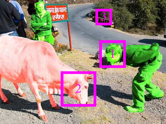
Figure 9: An illustration of the three firing types of mid-level elements. In the image, ground-truth object instances of the underlying category (e.g., “person”) are overlaid in green while instances of other categories (e.g., “cow”) are overlaid in red. Obviously, the firing (1) fires on the ground-truth object while firings (2) and (3) belong to object and scene context respectively.

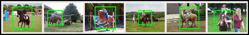
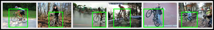
Figure 10: Detections of two object-context mid-level visual elements discovered from the “person” category on the Pascal VOC 2007 dataset.

6.4.1 Object and scene context

We first need to define context qualitatively. For this purpose, we leverage the test set of the segmentation challenge of the Pascal VOC 2007 dataset in which per-pixel labeling is available. Given a test image of a given object category, its ground-truth pixels annotations $S$ are categorized into the following three categories,

• $S_{gt}$: pixels belong to the underlying object category.

• $S_{ot}$: pixels belong to any of the rest $19$ object categories.

• $S_{sc}$: pixels belong to none of the $20$ object categories, i.e., belong to the background.

Accordingly, given a firing (i.e., predicted bounding box) $B$ of a mid-level visual element on an image, we compute an overlap ratio for each of the three types of pixels,

$$O_{gt}=\frac{|B\cap S_{gt}|}{|B|},O_{ot}=\frac{|B\cap S_{ot}|}{|B|},O_{sc}=\frac{|B\cap S_{sc}|}{|B|},$$ (6)

where $|\cdot|$ measures cardinality. Note that $O_{gt}+O_{ot}+O_{sc}=1$. By comparing the three types of overlap ratios, we can easily define three firing types, which includes two types of context firing and one ground-truth object firing,

• Scene context: if $O_{sc}>0.9$.

• Object context: if $O_{sc}<=0.9$ and $O_{ot}>O_{gt}$.

• Ground-truth object: if $O_{sc}<=0.9$ and $O_{ot}<O_{ht}$.

Fig. 9 depicts a visual example of the three firing types. In practice, for each image in the test set, we collect the predicted bounding box with the maximum detection score if there exists any positive detections (larger than a threshold), followed by categorizing it into one of the three types based on Eq. 6. Thus, a mid-level visual element is categorized into the three firing types based on its major votes of positive detections.

6.4.2 Analysis

Following the context definition in Sec. 6.4.1, we categorize the each of the top-$20$ discovered mid-level visual elements of each category of the Pascal VOC 2007 dataset into one of the three categories: gt-object, object or scene context. The distribution of this categorization is illustrated in Table 8.

Interestingly, for many classes, the majority of the discovered mid-level visual elements fires on the underlying object, and context information seems to be less important. More specifically, as shown in Table 8, mid-level visual elements in $10$ out of $20$ classes never capture context information, which reflects image patches capture context in these classes are neither representative nor discriminative. On average, more than $87\%$ mid-level visual element capture the underlying object across all the categories.

We also observe that contextual information from other object categories plays a important role for discovering mid-level visual element from person($60.0\%$), bottle($56.3\%$) and chair($45.0\%$). Fig. 10 shows two examples of object-context mid-level visual elements discovered from class person.

As depicted in Table 8, most categories have very low proportion of scene-context mid-level visual elements except for boat, which has a relatively high value of $35\%$.

We also compare distributions of mid-level elements discovered using different CNN models (Fig. 11). As shown in Fig. 11, for both CNN models, the majority consists of those mid-level elements tend to capture parts of ground-truth objects and contextual ones only constitute a relatively small fraction. Also, for mid-level visual elements capturing ground-truth objects, the fraction of those discovered from the VGG-VD model bypasses that from the CaffeRef model by $14\%$ ($88\%$ vs.$74\%$). We thus conjecture that for image classification, deeper CNNs will more likely to learn to represent the underlying objects and contextual information may not be that valuable.

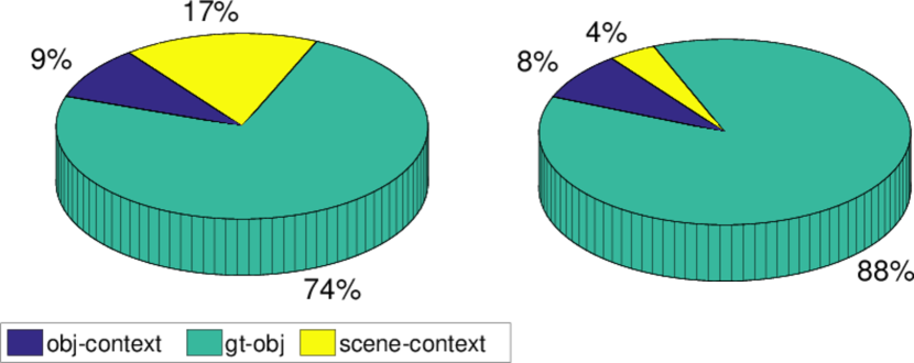
Figure 11: Distributions of mid-level visual elements discovered using different CNN models—CaffeRef (left) and VGG-VD (right).

7 Discussion

Recently, some works on accelerating CNNs [19, 72] advocate using binary activation values in CNNs. It would be interesting to try binary CNN features for creating transactions. In this case, for an image patch, all of its CNN dimensions with positive activation values will be kept to generate on transaction. This means we do not need to select the K largest activation magnitudes as in the current approach (Sec.4.2), and there will be no information loss for transaction creation at all.

As the feature dimension of the Bag-of-Elements representation (Sec. 5.2.2) is proportion to the number of categories, most of the current works on mid-level visual elements, including ours, cannot be applied to image classification datasets which contain a huge number of categories (e.g., ImageNet [21] and Places [100]). A good indication of future work to address this scalability issue may be using shared mid-level visual elements [63].

8 Conclusion and future work

We have addressed the task of mid-level visual element discovery from the perspective of pattern mining. More specifically, we have shown that CNN activation can be encoded into transactions, the data structure used by existing pattern mining techniques which can be readily applied to discover discriminative mid-level visual element candidates. We further develop different strategies to generate image representations from the mined visual element candidates. We experimentally demonstrate the effectiveness of the mined mid-level visual elements and achieve the state-of-the-art classification performance on various datasets by using the generated image representation.

Although this paper only addresses the image classification problem, our method can be extended to many other applications and serves as a bridge between visual recognition and pattern mining research fields. Since the publication of our conference paper [55], there have been several works [22, 65] which follow our approach to develop methods suited for various applications, including human action and attribute recognition [22] and modeling visual compatibility [65].

In future work, we plan to investigate three directions to extend our approach. Firstly, we will develop efficient mining methods to mine the patterns that are shared across categories. This will address the limitation of the current method that it can only detect discriminative patterns for each category and thus is not very scalable to a dataset with a huge number of categories, e.g., ImageNet. Secondly, we will extend our method to the metric learning setting. In such a setting, the mined discriminative patterns are only used to make a binary decision, that is, whether the input two images are from the same category. Finally, we will apply our method to more applications, especially those that can leverage the state-of-the-art pattern mining techniques.

References

- [1] A. Agarwal and B. Triggs. Multilevel image coding with hyperfeatures. Int. J. Comp. Vis., 78(1):15–27, 2008.
- [2] P. Agrawal, R. Girshick, and J. Malik. Analyzing the performance of multilayer neural networks for object recognition. In Proc. Eur. Conf. Comp. Vis., pages 329–344, 2014.
- [3] R. Agrawal and R. Srikant. Fast algorithms for mining association rules in large databases. In Proc. Int. Conf. Very Large Databases, pages 487–499, 1994.
- [4] M. Aubry, D. Maturana, A. A. Efros, B. C. Russell, and J. Sivic. Seeing 3d chairs: exemplar part-based 2d-3d alignment using a large dataset of cad models. In Proc. IEEE Conf. Comp. Vis. Patt. Recogn., pages 3762–3769, 2014.
- [5] M. Aubry, B. C. Russell, and J. Sivic. Painting-to-3d model alignment via discriminative visual elements. Proc. Ann. ACM SIGIR Conf., 33(2):14, 2014.
- [6] H. Azizpour, A. S. Razavian, J. Sullivan, A. Maki, and S. Carlsson. Factors of transferability for a generic convnet representation. IEEE Trans. Pattern Anal. Mach. Intell., 2016.
- [7] A. Bansal, A. Shrivastava, C. Doersch, and A. Gupta. Mid-level elements for object detection. arXiv preprint arXiv:1504.07284, 2015.
- [8] C. Borgelt. Frequent item set mining. Wiley Interdisc. Rew.: Data Mining and Knowledge Discovery, 2(6):437–456, 2012.
- [9] L. Bossard, M. Guillaumin, and L. V. Gool. Food-101 – mining discriminative components with random forests. In Proc. Eur. Conf. Comp. Vis., pages 446–461, 2014.
- [10] L. D. Bourdev, S. Maji, T. Brox, and J. Malik. Detecting people using mutually consistent poselet activations. In Proc. Eur. Conf. Comp. Vis., pages 168–181, 2010.
- [11] L. D. Bourdev, S. Maji, and J. Malik. Describing people: A poselet-based approach to attribute classification. In Proc. IEEE Int. Conf. Comp. Vis., pages 1543–1550, 2011.
- [12] L. D. Bourdev and J. Malik. Poselets: Body part detectors trained using 3d human pose annotations. In Proc. IEEE Int. Conf. Comp. Vis., pages 1365–1372, 2009.
- [13] Y. Boureau, F. R. Bach, Y. LeCun, and J. Ponce. Learning mid-level features for recognition. In Proc. IEEE Conf. Comp. Vis. Patt. Recogn., 2010.
- [14] K. Chatfield, K. Simonyan, A. Vedaldi, and A. Zisserman. Return of the devil in the details: Delving deep into convolutional nets. In Proc. Brit. Mach. Vis. Conf., 2014.
- [15] H. Cheng, X. Yan, J. Han, and P. S. Yu. Direct discriminative pattern mining for effective classification. In Proc. IEEE Int. Conf. Data Engr., pages 169–178, 2008.
- [16] M. J. Choi, A. Torralba, and A. S. Willsky. A tree-based context model for object recognition. IEEE Trans. Pattern Anal. Mach. Intell., 34(2):240–252, 2012.
- [17] M. Cimpoi, S. Maji, I. Kokkinos, and A. Vedaldi. Deep filter banks for texture recognition, description, and segmentation. Int. J. Comp. Vis., 118(1):65–94, 2016.
- [18] M. Cimpoi, S. Maji, and A. Vedaldi. Deep filter banks for texture recognition and segmentation. In Proc. IEEE Conf. Comp. Vis. Patt. Recogn., pages 3828–3836, 2015.
- [19] M. Courbariaux and Y. Bengio. Binarynet: Training deep neural networks with weights and activations constrained to+ 1 or-1. arXiv preprint arXiv:1602.02830, 2016.
- [20] E. Crowley and A. Zisserman. The state of the art: Object retrieval in paintings using discriminative regions. In Proc. Brit. Mach. Vis. Conf., 2014.
- [21] J. Deng, W. Dong, R. Socher, L.-J. Li, K. Li, and F.-F. Li. Imagenet: A large-scale hierarchical image database. In Proc. IEEE Conf. Comp. Vis. Patt. Recogn., pages 248–255, 2009.
- [22] A. Diba, A. M. Pazandeh, H. Pirsiavash, and L. V. Gool. Deepcamp: Deep convolutional action & attribute mid-level patterns. In Proc. IEEE Conf. Comp. Vis. Patt. Recogn., 2016.
- [23] S. K. Divvala, D. Hoiem, J. Hays, A. A. Efros, and M. Hebert. An empirical study of context in object detection. In Proc. IEEE Conf. Comp. Vis. Patt. Recogn., pages 1271–1278, 2009.
- [24] C. Doersch, A. Gupta, and A. A. Efros. Mid-level visual element discovery as discriminative mode seeking. In Proc. Adv. Neural Inf. Process. Syst., pages 494–502, 2013.
- [25] C. Doersch, S. Singh, A. Gupta, J. Sivic, and A. A. Efros. What makes paris look like paris? Proc. Ann. ACM SIGIR Conf., 31(4):101, 2012.
- [26] A. Dosovitskiy and T. Brox. Inverting visual representations with convolutional networks. In Proc. IEEE Conf. Comp. Vis. Patt. Recogn., 2016.
- [27] I. Endres, K. J. Shih, J. Jiaa, and D. Hoiem. Learning collections of part models for object recognition. In Proc. IEEE Conf. Comp. Vis. Patt. Recogn., pages 939–946, 2013.
- [28] M. Everingham, S. M. A. Eslami, L. V. Gool, C. K. I. Williams, J. M. Winn, and A. Zisserman. The pascal visual object classes challenge: A retrospective. Int. J. Comp. Vis., 111(1):98–136, 2015.
- [29] M. Everingham, L. J. V. Gool, C. K. I. Williams, J. M. Winn, and A. Zisserman. The pascal visual object classes (VOC) challenge. Int. J. Comp. Vis., 88(2):303–338, 2010.
- [30] R.-E. Fan, K.-W. Chang, C.-J. Hsieh, X.-R. Wang, and C.-J. Lin. Liblinear: A library for large linear classification. J. Mach. Learn. Res., 9:1871–1874, 2008.
- [31] P. F. Felzenszwalb, R. B. Girshick, D. A. McAllester, and D. Ramanan. Object detection with discriminatively trained part-based models. IEEE Trans. Pattern Anal. Mach. Intell., 32(9):1627–1645, 2010.
- [32] B. Fernando, É. Fromont, and T. Tuytelaars. Effective use of frequent itemset mining for image classification. In Proc. Eur. Conf. Comp. Vis., pages 214–227, 2012.
- [33] B. Fernando, É. Fromont, and T. Tuytelaars. Mining mid-level features for image classification. Int. J. Comp. Vis., 108(3):186–203, 2014.
- [34] B. Fernando and T. Tuytelaars. Mining multiple queries for image retrieval: On-the-fly learning of an object-specific mid-level representation. In Proc. IEEE Int. Conf. Comp. Vis., pages 2544–2551, 2013.
- [35] D. F. Fouhey, A. Gupta, and M. Hebert. Data-driven 3d primitives for single image understanding. In Proc. IEEE Int. Conf. Comp. Vis., pages 3392–3399, 2013.
- [36] D. F. Fouhey, W. Hussain, A. Gupta, and M. Hebert. Single image 3d without a single 3d image. In Proc. IEEE Int. Conf. Comp. Vis., pages 1053–1061, 2015.
- [37] Y. Gao, O. Beijbom, N. Zhang, and T. Darrell. Compact bilinear pooling. In Proc. IEEE Conf. Comp. Vis. Patt. Recogn., 2016.
- [38] A. Gilbert and R. Bowden. Data mining for action recognition. In Proc. Asian Conf. Comp. Vis., pages 290–303, 2014.
- [39] A. Gilbert, J. Illingworth, and R. Bowden. Action recognition using mined hierarchical compound features. IEEE Trans. Pattern Anal. Mach. Intell., 33(5):883–897, 2011.
- [40] R. Girshick, J. Donahue, T. Darrell, and J. Malik. Rich feature hierarchies for accurate object detection and semantic segmentation. In Proc. IEEE Conf. Comp. Vis. Patt. Recogn., pages 580–587, 2014.
- [41] R. B. Girshick, J. Donahue, T. Darrell, and J. Malik. Region-based convolutional networks for accurate object detection and segmentation. IEEE Trans. Pattern Anal. Mach. Intell., 38(1):142–158, 2016.
- [42] Y. Gong, L. Wang, R. Guo, and S. Lazebnik. Multi-scale orderless pooling of deep convolutional activation features. In Proc. Eur. Conf. Comp. Vis., pages 392–407, 2014.
- [43] G. Grahne and J. Zhu. Fast algorithms for frequent itemset mining using fp-trees. IEEE Trans. Knowl. Data Eng., 17(10):1347–1362, 2005.
- [44] B. Hariharan, J. Malik, and D. Ramanan. Discriminative decorrelation for clustering and classification. In Proc. Eur. Conf. Comp. Vis., pages 459–472, 2012.
- [45] K. He, X. Zhang, S. Ren, and J. Sun. Spatial pyramid pooling in deep convolutional networks for visual recognition. IEEE Trans. Pattern Anal. Mach. Intell., 37(9):1904–1916, 2015.
- [46] D. Hoiem, A. A. Efros, and M. Hebert. Putting objects in perspective. Int. J. Comp. Vis., 80(1):3–15, 2008.
- [47] A. Jain, A. Gupta, M. Rodriguez, and L. S. Davis. Representing videos using mid-level discriminative patches. In Proc. IEEE Conf. Comp. Vis. Patt. Recogn., pages 2571–2578, 2013.
- [48] H. Jegou, M. Douze, C. Schmid, and P. Pérez. Aggregating local descriptors into a compact image representation. In Proc. IEEE Conf. Comp. Vis. Patt. Recogn., pages 3304–3311, 2010.
- [49] Y. Jia, E. Shelhamer, J. Donahue, S. Karayev, J. Long, R. Girshick, S. Guadarrama, and T. Darrell. Caffe: Convolutional architecture for fast feature embedding. arXiv preprint arXiv:1408.5093, 2014.
- [50] M. Juneja, A. Vedaldi, C. V. Jawahar, and A. Zisserman. Blocks that shout: Distinctive parts for scene classification. In Proc. IEEE Conf. Comp. Vis. Patt. Recogn., pages 923–930, 2013.
- [51] A. Krizhevsky, I. Sutskever, and G. E. Hinton. Imagenet classification with deep convolutional neural networks. In Proc. Adv. Neural Inf. Process. Syst., pages 1106–1114, 2012.
- [52] S. Lazebnik, C. Schmid, and J. Ponce. Beyond bags of features: Spatial pyramid matching for recognizing natural scene categories. In Proc. IEEE Conf. Comp. Vis. Patt. Recogn., pages 2169–2178, 2006.
- [53] Y. J. Lee, A. A. Efros, and M. Hebert. Style-aware mid-level representation for discovering visual connections in space and time. In Proc. IEEE Int. Conf. Comp. Vis., pages 1857–1864, 2013.
- [54] Q. Li, J. Wu, and Z. Tu. Harvesting mid-level visual concepts from large-scale internet images. In Proc. IEEE Conf. Comp. Vis. Patt. Recogn., pages 851–858, 2013.
- [55] Y. Li, L. Liu, C. Shen, and A. van den Hengel. Mid-level deep pattern mining. In Proc. IEEE Conf. Comp. Vis. Patt. Recogn., pages 971–980, 2015.
- [56] T. Lin, A. RoyChowdhury, and S. Maji. Bilinear CNN models for fine-grained visual recognition. In Proc. IEEE Int. Conf. Comp. Vis., pages 1449–1457, 2015.
- [57] L. Liu, C. Shen, and A. van den Hengel. The treasure beneath convolutional layers: Cross convolutional layer pooling for image classification. In Proc. IEEE Conf. Comp. Vis. Patt. Recogn., pages 4749–4757, 2015.
- [58] L. Liu, C. Shen, L. Wang, A. van den Hengel, and C. Wang. Encoding high dimensional local features by sparse coding based fisher vectors. In Proc. Adv. Neural Inf. Process. Syst., pages 1143–1151, 2014.
- [59] L. Liu and L. Wang. What has my classifier learned? visualizing the classification rules of bag-of-feature model by support region detection. In Proc. IEEE Conf. Comp. Vis. Patt. Recogn., pages 3586–3593, 2012.
- [60] T. Malisiewicz and A. A. Efros. Beyond categories: The visual memex model for reasoning about object relationships. In Proc. Adv. Neural Inf. Process. Syst., pages 1222–1230, 2009.
- [61] T. Malisiewicz, A. Gupta, and A. A. Efros. Ensemble of exemplar-svms for object detection and beyond. In Proc. IEEE Int. Conf. Comp. Vis., pages 89–96, 2011.
- [62] K. Matzen and N. Snavely. Bubblenet: Foveated imaging for visual discovery. In Proc. IEEE Int. Conf. Comp. Vis., pages 1931–1939, 2015.
- [63] P. Mettes, J. C. van Gemert, and C. G. M. Snoek. No spare parts: Sharing part detectors for image categorization. Comp. Vis. Image Understanding, 2016.
- [64] M. Oquab, L. Bottou, I. Laptev, and J. Sivic. Learning and transferring mid-level image representations using convolutional neural networks. In Proc. IEEE Conf. Comp. Vis. Patt. Recogn., pages 1717–1724, 2014.
- [65] J. Oramas and T. Tuytelaars. Modeling visual compatibility through hierarchical mid-level elements. arXiv preprint arXiv:1604.00036, 2016.
- [66] A. Owens, J. Xiao, A. Torralba, and W. T. Freeman. Shape anchors for data-driven multi-view reconstruction. In Proc. IEEE Int. Conf. Comp. Vis., pages 33–40, 2013.
- [67] S. N. Parizi, A. Vedaldi, A. Zisserman, and P. Felzenszwalb. Automatic discovery and optimization of parts for image classification. In Proc. Int. Conf. Learn. Repr., 2015.
- [68] F. Perronnin, Y. Liu, J. Sánchez, and H. Poirier. Large-scale image retrieval with compressed fisher vectors. In Proc. IEEE Conf. Comp. Vis. Patt. Recogn., pages 3384–3391, 2010.
- [69] F. Perronnin, J. Sánchez, and T. Mensink. Improving the fisher kernel for large-scale image classification. In Proc. Eur. Conf. Comp. Vis., pages 143–156, 2010.
- [70] T. Quack, V. Ferrari, B. Leibe, and L. J. V. Gool. Efficient mining of frequent and distinctive feature configurations. In Proc. IEEE Int. Conf. Comp. Vis., pages 1–8, 2007.
- [71] A. Quattoni and A. Torralba. Recognizing indoor scenes. In Proc. IEEE Conf. Comp. Vis. Patt. Recogn., pages 413–420, 2009.
- [72] M. Rastegari, V. Ordonez, J. Redmon, and A. Farhadi. Xnor-net: Imagenet classification using binary convolutional neural networks. arXiv preprint arXiv:1603.05279, 2016.
- [73] A. S. Razavian, H. Azizpour, J. Sullivan, and S. Carlsson. Cnn features off-the-shelf: An astounding baseline for recognition. In Proc. IEEE Conf. Comp. Vis. Patt. Recogn. Workshops, pages 512–519, 2014.
- [74] K. Rematas, B. Fernando, F. Dellaert, and T. Tuytelaars. Dataset fingerprints: Exploring image collections through data mining. In Proc. IEEE Conf. Comp. Vis. Patt. Recogn., pages 4867–4875, 2015.
- [75] O. Russakovsky, J. Deng, H. Su, J. Krause, S. Satheesh, S. Ma, Z. Huang, A. Karpathy, A. Khosla, M. S. Bernstein, A. C. Berg, and L. Fei-Fei. Imagenet large scale visual recognition challenge. Int. J. Comp. Vis., 115(3):211–252, 2015.
- [76] K. J. Shih, I. Endres, and D. Hoiem. Learning discriminative collections of part detectors for object recognition. IEEE Trans. Pattern Anal. Mach. Intell., 37(8):1571–1584, 2015.
- [77] A. Shrivastava, T. Malisiewicz, A. Gupta, and A. A. Efros. Data-driven visual similarity for cross-domain image matching. Proc. Ann. ACM SIGIR Conf., 30(6):154, 2011.
- [78] K. Simonyan, A. Vedaldi, and A. Zisserman. Deep fisher networks for large-scale image classification. In Proc. Adv. Neural Inf. Process. Syst., pages 163–171, 2013.
- [79] K. Simonyan and A. Zisserman. Very deep convolutional networks for large-scale image recognition. In Proc. Int. Conf. Learn. Repr., 2015.
- [80] S. Singh, A. Gupta, and A. A. Efros. Unsupervised discovery of mid-level discriminative patches. In Proc. Eur. Conf. Comp. Vis., pages 73–86, 2012.
- [81] J. Sivic and A. Zisserman. Video google: A text retrieval approach to object matching in videos. In Proc. IEEE Int. Conf. Comp. Vis., pages 1470–1477, 2003.
- [82] H. O. Song, Y. J. Lee, S. Jegelka, and T. Darrell. Weakly-supervised discovery of visual pattern configurations. In Proc. Adv. Neural Inf. Process. Syst., pages 1637–1645, 2014.
- [83] J. Sun and J. Ponce. Learning discriminative part detectors for image classification and cosegmentation. In Proc. IEEE Int. Conf. Comp. Vis., pages 3400–3407, 2013.
- [84] J. Sun and J. Ponce. Learning dictionary of discriminative part detectors for image categorization and cosegmentation. Int. J. Comp. Vis., pages 1–23, 2016.
- [85] A. Torralba. Contextual priming for object detection. Int. J. Comp. Vis., 53(2):169–191, 2003.
- [86] T. Uno, T. Asai, Y. Uchida, and H. Arimura. LCM: an efficient algorithm for enumerating frequent closed item sets. In FIMI, 2003.
- [87] W. Voravuthikunchai, B. Crémilleux, and F. Jurie. Histograms of pattern sets for image classification and object recognition. In Proc. IEEE Conf. Comp. Vis. Patt. Recogn., pages 224–231, 2014.
- [88] J. Vreeken, M. van Leeuwen, and A. Siebes. Krimp: mining itemsets that compress. Data Min. Knowl. Discov., 23(1):169–214, 2011.
- [89] J. Wang, Z. Liu, Y. Wu, and J. Yuan. Learning actionlet ensemble for 3d human action recognition. IEEE Trans. Pattern Anal. Mach. Intell., 36(5):914–927, 2014.
- [90] J. Wang, Y. Yang, J. Mao, Z. Huang, and C. H. W. Xu. Cnn–rnn: A unified framework for multi-label image classification. In Proc. IEEE Conf. Comp. Vis. Patt. Recogn., 2016.
- [91] L. Wang, Y. Qiao, and X. Tang. Motionlets: Mid-level 3d parts for human motion recognition. In Proc. IEEE Conf. Comp. Vis. Patt. Recogn., pages 2674–2681, 2013.
- [92] X. Wang, B. Wang, X. Bai, W. Liu, and Z. Tu. Max-margin multiple-instance dictionary learning. In Proc. Int. Conf. Mach. Learn., pages 846–854, 2013.
- [93] Y. Wang, J. Choi, V. I. Morariu, and L. S. Davis. Mining discriminative triplets of patches for fine-grained classification. In Proc. IEEE Conf. Comp. Vis. Patt. Recogn., 2016.
- [94] Y. Wei, W. Xia, J. Huang, B. Ni, J. Dong, Y. Zhao, and S. Yan. CNN: single-label to multi-label. CoRR, abs/1406.5726, 2014.
- [95] B. Yao and L. Fei-Fei. Grouplet: A structured image representation for recognizing human and object interactions. In Proc. IEEE Conf. Comp. Vis. Patt. Recogn., pages 9–16, 2010.
- [96] D. Yoo, S. Park, J.-Y. Lee, and I. S. Kweon. Multi-scale pyramid pooling for deep convolutional representation. In Proc. IEEE Conf. Comp. Vis. Patt. Recogn. Workshops, pages 71–80, 2015.
- [97] J. Yuan, Y. Wu, and M. Yang. Discovery of collocation patterns: from visual words to visual phrases. In Proc. IEEE Conf. Comp. Vis. Patt. Recogn., 2007.
- [98] M. D. Zeiler and R. Fergus. Visualizing and understanding convolutional networks. In Proc. Eur. Conf. Comp. Vis., pages 818–833, 2014.
- [99] R. Zhao, W. Ouyang, and X. Wang. Learning mid-level filters for person re-identification. In Proc. IEEE Conf. Comp. Vis. Patt. Recogn., pages 144–151, 2014.
- [100] B. Zhou, À. Lapedriza, J. Xiao, A. Torralba, and A. Oliva. Learning deep features for scene recognition using places database. In Proc. Adv. Neural Inf. Process. Syst., pages 487–495, 2014.