Lipschitz Metrics for a Class of Nonlinear Wave Equations

Abstract

The nonlinear wave equation $u_{tt}-c(u)(c(u)u_{x})_{x}=0$ determines a flow of conservative solutions taking values in the space $H^{1}({\mathbb{R}})$. However, this flow is not continuous w.r.t. the natural $H^{1}$ distance. Aim of this paper is to construct a new metric which renders the flow uniformly Lipschitz continuous on bounded subsets of $H^{1}({\mathbb{R}})$. For this purpose, $H^{1}$ is given the structure of a Finsler manifold, where the norm of tangent vectors is defined in terms of an optimal transportation problem. For paths of piecewise smooth solutions, one can carefully estimate how the weighted length grows in time. By the generic regularity result proved in [7], these piecewise regular paths are dense and can be used to construct a geodesic distance with the desired Lipschitz property.

1 Introduction

Aim of this paper is to understand the continuous dependence of solutions to the nonlinear wave equation

$$u_{tt}-c(u)\bigl{(}c(u)u_{x}\bigr{)}_{x}~{}=~{}0\,.$$ (1.1)

Roughly speaking, the analysis in [8, 17, 22] shows that conservative solutions are unique, globally defined, and yield a flow on the space of couples $(u,u_{t})\in H^{1}({\mathbb{R}})\times{\bf L}^{2}({\mathbb{R}})$. For each conservative solution, the total energy

$$E(t)~{}\doteq~{}\int\bigl{[}u_{t}^{2}+c^{2}(u)\,u_{x}^{2}\bigr{]}\,dx$$ (1.2)

remains constant in time. Precise results in this direction will be recalled in Section 2. On the other hand, these solutions do not depend continuously on the initial data, w.r.t. the distance in the normed space $H^{1}\times{\bf L}^{2}$.

In the present paper we construct a new distance functional which renders Lipschitz continuous the flow generated by (1.1). We recall that, for solutions of the Hunter-Saxton or the Camassa-Holm equation, a similar task was achieved in [10, 13, 14, 20, 21].

Developing ideas in [13], our distance will be determined by the minimum cost to transport an energy measure from one solution to the other. While all previous papers dealt with first order equations, to define a suitable transportation distance between two solutions $u,\tilde{u}$ of (1.1) one now faces three main difficulties:

• At any given time $t$, each solution determines two distinct measures. These account for the energy $\mu^{t}_{+}$ of forward moving waves and the energy $\mu_{t}^{-}$ of backward moving waves. The distance between $u(t)$ and $\tilde{u}(t)$ should be measured by the minimum cost for transporting $\mu^{t}_{+}$ to $\tilde{\mu}^{t}_{+}$ and $\mu^{t}_{-}$ to $\tilde{\mu}^{t}_{-}$.

• The above double transportation problem is considerably complicated by the fact that, while the total energy is conserved, some energy can be transferred from forward to backward moving waves, or viceversa. These source terms must be accounted for, when designing an “optimal double transportation plan”.

• As a wave front crosses waves of the opposite family, its speed can change. As a consequence, the distance between two corresponding fronts in $u$ and $\tilde{u}$ may quickly increase, making the optimal transportation plan more costly. To compensate for this effect, one needs to insert a weight function, accounting for the total energy of approaching waves.

In Section 3 we introduce a Finsler norm on tangent vectors, related to an energy transportation cost. Given a smooth path $\gamma:\theta\mapsto(u^{\theta},u_{t}^{\theta})$, one can then define its weighted length $\|\gamma\|$ by integrating the norm of the tangent vector $d\gamma/d\theta$. Proposition 1, stated in Section 3 and proved in Section 4, contains the key estimate, describing how the norm of a tangent vector grows in time. Assuming that, for $\theta\in[0,1]$ and $t\in[0,T]$, all solutions $u^{\theta}(t,\cdot)$ remain sufficiently regular so that the length of the path $\gamma^{t}:\theta\mapsto(u^{\theta}(t),u_{t}^{\theta}(t))$ can still be computed, we obtain the bound

$$\|\gamma^{t}\|~{}\leq~{}C_{T}\,\|\gamma^{0}\|\,,\qquad\qquad\hbox{for all }~{}t\in[0,T].$$ (1.3)

Here the constant $C_{T}$ depends only on $T$ and on a bound on the $H^{1}\times{\bf L}^{2}$ norm of the initial data. At this stage, it is natural to define the geodesic distance

$$d^{*}\Big{(}(u,u_{t})\,,~{}(\tilde{u},\tilde{u}_{t})\Big{)}~{}\doteq~{}\inf~{}\Big{\{}\|\gamma\|\,;~{}~{}~{}\gamma:[0,1]\mapsto H^{1}\times{\bf L}^{2}\,,\quad\gamma(0)=(u,u_{t}),~{}~{}\gamma(1)=(\tilde{u},\tilde{u}_{t})\Big{\}}.$$ (1.4)

By (1.3) we thus expect that, for any two solutions of (1.1) and any $t\in[0,T]$, this distance should satisfy

$$d^{*}\Big{(}(u(t),u_{t}(t))\,,~{}(\tilde{u}(t),\tilde{u}_{t}(t))\Big{)}~{}\leq~{}C_{T}\cdot d^{*}\Big{(}(u(0),u_{t}(0))\,,~{}(\tilde{u}(0),\tilde{u}_{t}(0))\Big{)}.$$ (1.5)

This would imply that solutions depend Lipschitz continuously on the initial data, in the distance $d^{*}$.

To clinch this argument, one major difficulty must be overcome. Indeed, smooth solutions may well develop singularities in finite time, [19]. Given a path $\gamma^{0}$ of smooth initial data, there is no guarantee that at any time $t\in[0,T]$ the path $\gamma^{t}$ will be regular enough so that the tangent vectors $d\gamma^{t}/d\theta$ are meaningfully defined (see Fig. 1). We remark that a similar issue was encountered in the analysis of hyperbolic conservation laws [6]. For a path of piecewise smooth solutions with finitely many shocks, a weighted norm on a suitable family of tangent vectors was introduced in [5]. However, a lengthy effort was later required [9, 12], in order to construct paths of approximate solutions which retained enough regularity, so that their length could still be estimated in terms of these tangent vectors.

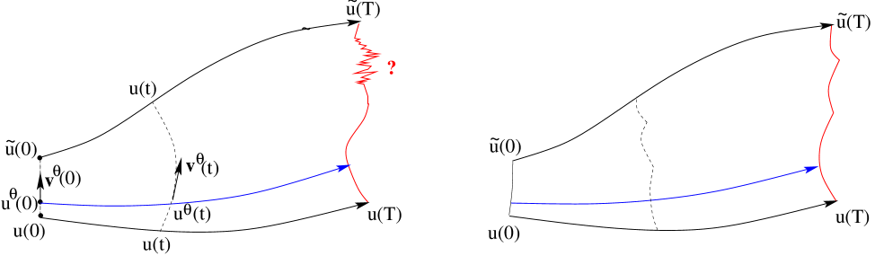
Figure 1: Left: due to singularity formation, a smooth path of initial data $\gamma^{0}:\theta\mapsto u^{\theta}(0)$ may lose regularity at a later time $T$. In this case, the weighted length $\|\gamma^{T}\|$ can no longer be computed by integrating the norm of a tangent vector. Right: by a small perturbation of the initial data, one obtains a path of solutions $\theta\mapsto u^{\theta}$ which remain piecewise smooth, for all except finitely many values of $\theta\in[0,1]$ .

In the present context, we can take advantage of the generic regularity results recently proved in [7]. These can be summarized as follows.

• For an open dense set of initial data

  $$(u(0,\cdot)\,,~{}u_{t}(0,\cdot))~{}=~{}(u_{0},u_{1})~{}\in~{}\Big{(}{\mathcal{C}}^{3}({\mathbb{R}})\cap H^{1}({\mathbb{R}})\Big{)}\times\Big{(}{\mathcal{C}}^{2}({\mathbb{R}})\cap{\bf L}^{2}({\mathbb{R}})\Big{)}$$ (1.6)

  the corresponding solution $u=u(t,x)$ of (1.1) is piecewise smooth in the $t$-$x$ plane, with singularities occurring along a finite set of smooth curves.

• Every path of initial data $\theta\mapsto\gamma^{0}(\theta)=(u_{0}^{\theta},u_{1}^{\theta})$ can be approximated by a second path $\theta\mapsto\tilde{\gamma}^{0}(\theta)=(\tilde{u}_{0}^{\theta},\tilde{u}_{1}^{\theta})$ such that, for all but finitely many values of $\theta\in[0,1]$, the corresponding solution $\tilde{u}^{\theta}$ remains piecewise smooth on the domain $[0,T]\times{\mathbb{R}}$.

Using this dense set of piecewise regular paths, we can thus define a geodesic distance on the space $H^{1}\times{\bf L}^{2}$, with the desired Lipschitz property. Our main results are contained in

• Proposition 1, which establishes the basic estimate (3.22) on the size of tangent vectors.

• Theorem 5, providing the bound (6.3) on how the length of a path of solutions can grow in time.

• Theorem 7, showing that, by (7.6), the flow generated by the wave equation (1.1) is Lipschitz continuous w.r.t. the geodesic distance $d^{*}$.

We remark that, for hyperbolic conservation laws, the distance constructed in [5, 9, 12] is equivalent to the ${\bf L}^{1}$ distance. On the contrary, our new metric is not equivalent to the norm distance on $H^{1}\times{\bf L}^{2}$. The completion of $H^{1}\times{\bf L}^{2}$ w.r.t. the geodesic distance includes a family of measures. This should not come as a surprise, since it was already observed in [17, 22] that conservative solutions can occasionally be measure-valued.

In Section 7 we compare the geodesic distance (1.4) with more familiar distances found in the literature. In one direction, we show that

$$d^{*}\Big{(}(u_{0},u_{1})\,,~{}(\tilde{u}_{0},\tilde{u}_{1})\Big{)}~{}\leq~{}C\cdot\Big{(}\|u_{0}-\tilde{u}_{0}\|_{H^{1}}+\|u_{0}-\tilde{u}_{0}\|_{W^{1.1}}+\|u_{1}-\tilde{u}_{1}\|_{{\bf L}^{2}}+\|u_{1}-\tilde{u}_{1}\|_{{\bf L}^{1}}\Big{)}\,,$$

for some constant $C$. On the other hand, let $\mu$ and $\tilde{\mu}$ be the positive measures having densities respectively

$$u_{t}^{2}+c^{2}(u)u_{x}^{2}\qquad\hbox{and}\qquad\tilde{u}_{t}^{2}+c^{2}(\tilde{u})\tilde{u}_{x}^{2}$$ (1.7)

w.r.t. Lebesgue measure. Then the geodesic distance $d^{*}$ dominates the Wasserstein distance between the two measures. Namely

$$\sup\,\left\{\bigg{|}\int f\,d\mu-\int fd\tilde{\mu}\bigg{|}\,;~{}~{}\|f\|_{{\mathcal{C}}^{1}}\leq 1\right\}~{}\leq~{}d^{*}\Big{(}(u,u_{t})\,,~{}(\tilde{u},\tilde{u}_{t})\Big{)}\,.$$ (1.8)

All of the present analysis is concerned with conservative solutions to (1.1). For dissipative solutions, studied in [15, 19, 26, 27], the continuous dependence for general initial data in $H^{1}\times{\bf L}^{2}$ remains an open question. For scalar conservation laws, an entirely different approach to continuous dependence, relying on an ${\bf L}^{2}$ formulation, was developed in [2, 3, 4].

2 Conservative solutions to the nonlinear wave equation

In this section we review the main results in [7, 8, 17] on the Cauchy problem for the quasilinear second order wave equation

$$u_{tt}-c(u)\big{(}c(u)u_{x}\big{)}_{x}=0\,,$$ (2.1)

with initial data

$$u(0,x)=u_{0}(x)\,,\qquad u_{t}(0,x)=u_{1}(x)\,.$$ (2.2)

Here $c:{\mathbb{R}}\mapsto{\mathbb{R}}_{+}$ is a smooth, uniformly positive function, such that

$$c(u)~{}\geq~{}c_{0}~{}>~{}0\,.$$ (2.3)

Consider the variables

$$\left\{\begin{array}[]{rcl}R&\doteq&u_{t}+c(u)u_{x}\,,\\ S&\doteq&u_{t}-c(u)u_{x}\,,\end{array}\right.$$ (2.4)

so that

$$u_{t}={R+S\over 2}\,,\qquad\qquad u_{x}={R-S\over 2c}\,.$$ (2.5)

By (2.1), the variables $R,S$ satisfy

$$\left\{\begin{array}[]{rcl}R_{t}-cR_{x}&=&{c^{\prime}\over 4c}(R^{2}-S^{2}),\\[8.53581pt] S_{t}+cS_{x}&=&{c^{\prime}\over 4c}(S^{2}-R^{2}).\end{array}\right.$$ (2.6)

Multiplying the first equation in (2.6) by $R$ and the second one by $S$, one obtains balance laws for $R^{2}$ and $S^{2}$, namely

$$\left\{\begin{array}[]{rcl}(R^{2})_{t}-(cR^{2})_{x}&=&{c^{\prime}\over 2c}(R^{2}S-RS^{2})\,,\\[8.53581pt] (S^{2})_{t}+(cS^{2})_{x}&=&-{c^{\prime}\over 2c}(R^{2}S-RS^{2})\,.\end{array}\right.$$ (2.7)

As a consequence, for smooth solutions the following quantity is conserved:

$$e~{}\doteq~{}u_{t}^{2}+c^{2}u_{x}^{2}~{}=~{}{R^{2}+S^{2}\over 2}\,.$$ (2.8)

We think of $R^{2}/2$ and $S^{2}/2$ as the energy of backward and forward moving waves, respectively. These are not separately conserved. Indeed, by (2.7) energy is transferred from forward to backward waves, and viceversa. The main results on the existence of solutions to the Cauchy problem can be summarized as follows. Theorem 1. Let $c:{\mathbb{R}}\mapsto{\mathbb{R}}$ be a smooth function satisfying (2.3). Assume that the initial data $u_{0}$ in (2.2) is absolutely continuous, and that $(u_{0})_{x}\in{\bf L}^{2}\,$,  $u_{1}\in{\bf L}^{2}$. Then the Cauchy problem (2.1)-(2.2) admits a weak solution $u=u(t,x)$, defined for all $(t,x)\in{\mathbb{R}}\times{\mathbb{R}}$. In the $t$-$x$ plane, the function $u$ is locally Hölder continuous with exponent $1/2$. This solution $t\mapsto u(t,\cdot)$ is continuously differentiable as a map with values in ${\bf L}^{p}_{\rm loc}$, for all $1\leq p<2$. Moreover, it is Lipschitz continuous w.r.t. the ${\bf L}^{2}$ distance, i.e.

$$\big{\|}u(t,\cdot)-u(s,\cdot)\big{\|}_{{\bf L}^{2}}~{}\leq~{}L\,|t-s|$$ (2.9)

for all $t,s\in{\mathbb{R}}$. The equation (2.1) is satisfied in distributional sense, i.e.

$$\int\!\!\int\Big{[}\phi_{t}\,u_{t}-\big{(}c(u)\phi\big{)}_{x}c(u)\,u_{x}\Big{]}\,dxdt~{}=~{}0$$ (2.10)

for all test functions $\phi\in{\mathcal{C}}^{1}_{c}$. The maps $t\mapsto u_{t}(t,\cdot)$ and $t\mapsto u_{x}(t,\cdot)$ are continuous with values in ${\bf L}^{p}_{loc}({\mathbb{R}})$, for every $p\in[1,2[\,$. Theorem 2. In the same setting as Theorem 1, a unique solution $u=u(t,x)$ exists which is conservative in the following sense.

There exists two families of positive Radon measures on the real line: $\{\mu_{-}^{t}\}$ and $\{\mu_{+}^{t}\}$, depending continuously on $t$ in the weak topology of measures, with the following properties.

• At every time $t$ one has

  $$\mu_{-}^{t}({\mathbb{R}})+\mu_{+}^{t}({\mathbb{R}})~{}=~{}E_{0}~{}\doteq~{}\int_{-\infty}^{\infty}\Big{[}u_{1}^{2}(x)+\bigl{(}c(u_{0}(x))u_{0,x}(x)\bigr{)}^{2}\Big{]}\,dx\,.$$ (2.11)

• For each $t$, the absolutely continuous parts of $\mu_{-}^{t}$ and $\mu_{+}^{t}$ w.r.t. the Lebesgue measure have densities respectively given by

  $$R^{2}~{}=~{}\bigl{(}u_{t}+c(u)u_{x}\bigr{)}^{2},\qquad\qquad S^{2}~{}=~{}\bigl{(}u_{t}-c(u)u_{x}\bigr{)}^{2}.$$ (2.12)

• For almost every $t\in{\mathbb{R}}$, the singular parts of $\mu^{t}_{-}$ and $\mu^{t}_{+}$ are concentrated on the set where $c^{\prime}(u)=0$.

• The measures $\mu_{-}^{t}$ and $\mu_{+}^{t}$ provide measure-valued solutions respectively to the balance laws

  $$\left\{\begin{array}[]{rcl}\xi_{t}-(c\xi)_{x}&=&{c^{\prime}\over 2c}(R^{2}S-RS^{2})\,,\\[8.53581pt] \eta_{t}+(c\eta)_{x}&=&-{c^{\prime}\over 2c}(R^{2}S-RS^{2})\,.\end{array}\right.$$ (2.13)

The existence part of the above theorems was proved in [17]. The uniqueness of conservative solutions has been recently established in [8]. Remark 1. By (2.13) the total energy, represented by the positive measure $\mu^{t}=\mu^{t}_{+}+\mu^{t}_{-}$, is conserved in time. Occasionally, some of this energy is concentrated on a set of measure zero. At a time $\tau$ when this happens, $\mu^{\tau}$ has a non-trivial singular part and hence its absolutely continuous part satisfies

$$\int\Big{[}u_{t}^{2}(\tau,x)+c^{2}\big{(}u(\tau,x)\big{)}\,u_{x}^{2}(\tau,x)\Big{]}\,dx~{}<~{}E_{0}\,.$$

The condition (iii) puts some restrictions on the set of such times $\tau$. In particular, if $c^{\prime}(u)\not=0$ for all $u$, then this set has measure zero. Remark 2. For any $t\geq 0$, the conservation of the total energy implies

$$\|u_{t}(t)\|^{2}_{{\bf L}^{2}}~{}\leq~{}E_{0}~{}\doteq~{}\int(u_{1}^{2}+c^{2}(u_{0})u^{2}_{0,x})\,dx\,.$$ (2.14)

Hence (2.9) holds with Lipschitz constant $L=\sqrt{E_{0}}$. Moreover, one has the bounds

$$\|u(t,\cdot)\|_{{\bf L}^{2}}~{}\leq~{}\|u_{0}\|_{{\bf L}^{2}}+t\,\sqrt{E_{0}}\,,\qquad\qquad\|u_{x}(t,\cdot)\|_{{\bf L}^{2}}~{}\leq~{}{\sqrt{E_{0}}\over c_{0}}\,.$$ (2.15)

This yields an a priori bound on $\|u(t,\cdot)\|_{H^{1}}$, and hence on $\|u(t,\cdot)\|_{L^{\infty}}$, depending only on time and on the total energy $E_{0}$. In turn, since the wave speed $c(\cdot)$ is smooth, we obtain an a priori bound on $c(u)$ and $|c^{\prime}(u)|$.

3 First order variations

For simplicity, in this section we consider solutions of (2.1) with bounded support. More precisely, we shall assume that all our solutions satisfy

$$u(t,x)~{}=~{}0\qquad\qquad\hbox{for}~{}x\notin[0,L_{0}],\quad t\in[0,T].$$ (3.1)

Because of finite propagation speed, this is hardly a restriction.

Let $(u,R,S)$ provide a smooth solution to (2.1), (2.4), and consider a family of perturbed solutions of the form

$$u^{\varepsilon}~{}=~{}u+\varepsilon v+o(\varepsilon)\,,\qquad\qquad\left\{\begin{array}[]{rl}R^{\varepsilon}&=~{}R+\varepsilon r+o(\varepsilon)\,,\cr S^{\varepsilon}&=~{}S+\varepsilon s+o(\varepsilon)\,.\end{array}\right.$$ (3.2)

From (2.5) it follows

$$u^{\varepsilon}_{t}~{}=~{}{R^{\varepsilon}+S^{\varepsilon}\over 2}~{}=~{}{R+S\over 2}+\varepsilon{r+s\over 2}+o(\varepsilon)\,,$$ (3.3)

$$u^{\varepsilon}_{x}~{}=~{}{R^{\varepsilon}-S^{\varepsilon}\over 2c(u^{\varepsilon})}~{}=~{}{R-S\over 2c(u)}+\varepsilon{r-s\over 2c(u)}-\varepsilon{R-S\over 2c^{2}(u)}c^{\prime}(u)\,v+o(\varepsilon)\,.$$ (3.4)

Under the assumption (3.1), given $r,s$, the perturbation $v$ is uniquely determined by

$$v_{x}~{}=~{}-{(R-S)c^{\prime}(u)\over 2c^{2}(u)}\,v+{r-s\over 2c(u)}\,,\qquad\qquad v(t,0)~{}=~{}0\,.$$ (3.5)

Furthermore, we have

$$v_{t}~{}=~{}{r+s\over 2}\,.$$ (3.6)

A direct computation shows that the first order perturbations $v,s,r$ satisfy the linear equations

$$v_{tt}-c^{2}v_{xx}~{}=~{}{2cc^{\prime}u_{x}v_{x}}+\Big{(}(c^{\prime})^{2}u_{x}^{2}+cc^{\prime\prime}u_{x}^{2}+2cc^{\prime}u_{xx}\Big{)}v\,.$$ (3.7)

$$\left\{\begin{array}[]{rl}r_{t}-c(u)r_{x}&\displaystyle=~{}c^{\prime}R_{x}v+\left({c^{\prime\prime}\over 4c}-{(c^{\prime})^{2}\over 4c^{2}}\right)(R^{2}-S^{2})v+{c^{\prime}\over 2c}(Rr-Ss)\,,\cr&\cr s_{t}+c(u)s_{x}&\displaystyle=~{}-c^{\prime}S_{x}v+\left({c^{\prime\prime}\over 4c}-{(c^{\prime})^{2}\over 4c^{2}}\right)(S^{2}-R^{2})v+{c^{\prime}\over 2c}(Ss-Rr)\,.\end{array}\right.$$ (3.8)

By the assumptions (2.3) on the wave speed $c(u)$, all functions $c^{\prime}/4c$, $c^{\prime\prime}/4c$, $(c^{\prime})^{2}/4c^{2}$, are smooth functions of $u$. We shall introduce a weighted norm on tangent vectors $r,s$, which takes into account the total energy of waves which are approaching a given wave located at $x$. This is described by the weights

$${\mathcal{W}}^{-}(x)~{}\doteq~{}\displaystyle 1+\int^{x}_{-\infty}S^{2}(y)\,dy\,,\qquad\qquad{\mathcal{W}}^{+}(x)~{}\doteq~{}\displaystyle 1+\int_{x}^{+\infty}R^{2}(y)\,dy\,.$$ (3.9)

In addition, consider the function

$$a(t)~{}\doteq~{}\int_{-\infty}^{\infty}\frac{|c^{\prime}|\,\bigl{|}R^{2}S-S^{2}R\bigr{|}}{2c}(t,x)~{}dx.$$ (3.10)

As proved in [8], the function

$$\tau~{}\mapsto~{}\int_{0}^{\tau}\int_{-\infty}^{+\infty}\left|\frac{c^{\prime}}{2c}(R^{2}S-RS^{2})\right|(t,x)\,dx\,dt$$

is Hölder continuous and absolutely continuous on bounded time intervals, and has sub-linear growth. In particular (see (3.11)-(3.12) in the proof of Lemma 1 in [8]), one has

$$\int_{0}^{T}a(t)\,dt~{}\leq~{}C_{T}\,,$$ (3.11)

for some constant $C_{T}$ depending only on $T$ and on the total energy $E_{0}$. By (2.7) it follows

$$\left\{\begin{array}[]{rl}{\mathcal{W}}^{-}_{t}-c{\mathcal{W}}^{-}_{x}&\displaystyle=~{}-2cS^{2}+\int^{x}_{-\infty}\frac{c^{\prime}}{2c}(S^{2}R-R^{2}S)~{}dy~{}\leq~{}-2c_{0}S^{2}+a(t),\cr\cr{\mathcal{W}}^{+}_{t}+c{\mathcal{W}}^{+}_{x}&\displaystyle=~{}-2cR^{2}+\int^{+\infty}_{x}\frac{c^{\prime}}{2c}(R^{2}S-S^{2}R)~{}dy~{}\leq~{}-2c_{0}R^{2}+a(t)\,.\end{array}\right.$$ (3.12)

On the space of tangent vectors $(v,r,s)$ we introduce a Finsler norm, having the form

$$\Big{\|}(v,\,r,\,s)\Big{\|}_{(u,R,S)}~{}\doteq~{}\inf_{\tilde{r},\tilde{s},w,z}\Big{\|}(\tilde{r},w,\tilde{s},z)\Big{\|}_{(u,R,S)}\,,$$ (3.13)

where the infimum is taken over the set of vertical displacements $\tilde{r},\tilde{s}$ and shifts $w,z$ which satisfy

$$\left\{\begin{array}[]{rl}r&=~{}\tilde{r}-wR_{x}+{c^{\prime}\over 8c^{2}}(w-z)S^{2}\,,\cr\cr s&=~{}\tilde{s}-zS_{x}+{c^{\prime}\over 8c^{2}}(w-z)R^{2}\,.\end{array}\right.$$ (3.14)

This norm is defined as

$$\begin{array}[]{l}\Big{\|}(\tilde{r},w,\tilde{s},z)\Big{\|}_{(u,R,S)}\cr\cr\doteq\displaystyle~{}\kappa_{1}\int\Big{\{}|w|\bigl{(}1+R^{2}\bigr{)}{\mathcal{W}}^{-}+|z|\bigl{(}1+S^{2}\bigr{)}{\mathcal{W}}^{+}\Big{\}}dx\cr\cr\quad\displaystyle+\kappa_{2}\int\Big{\{}|\tilde{r}|{\mathcal{W}}^{-}+|\tilde{s}|{\mathcal{W}}^{+}\Big{\}}dx\cr\cr\quad\displaystyle+\kappa_{3}\int\Big{|}v+\frac{Rw}{2c}-\frac{Sz}{2c}\Big{|}\,\bigg{\{}(1+R^{2})\,{\mathcal{W}}^{-}+(1+S^{2})\,{\mathcal{W}}^{+}\bigg{\}}dx\cr\cr\quad\displaystyle+\kappa_{4}\int\bigg{\{}\Big{|}w_{x}+\frac{c^{\prime}}{4c^{2}}(w-z)S\Big{|}{\mathcal{W}}^{-}+\Big{|}z_{x}+\frac{c^{\prime}}{4c^{2}}(w-z)R\Big{|}{\mathcal{W}}^{+}\bigg{\}}dx\cr\cr\quad\displaystyle+\kappa_{5}\int\bigg{\{}\Big{|}Rw_{x}+\frac{c^{\prime}}{4c^{2}}(w-z)SR\Big{|}{\mathcal{W}}^{-}+\Big{|}Sz_{x}+\frac{c^{\prime}}{4c^{2}}(w-z)RS\Big{|}{\mathcal{W}}^{+}\bigg{\}}dx\cr\cr\displaystyle\quad+\kappa_{6}\int\bigg{\{}\Big{|}2R\tilde{r}+R^{2}w_{x}+\frac{c^{\prime}}{4c^{2}}R^{2}S(w-z)\Big{|}{\mathcal{W}}^{-}+\Big{|}2S\tilde{s}+S^{2}z_{x}+\frac{c^{\prime}}{4c^{2}}S^{2}R(w-z)\Big{|}{\mathcal{W}}^{+}\bigg{\}}dx\cr\cr\doteq~{}\kappa_{1}I_{1}+\kappa_{2}I_{2}+\kappa_{3}I_{3}+\kappa_{4}I_{4}+\kappa_{5}I_{5}+\kappa_{6}I_{6}\,,\end{array}$$ (3.15)

for suitable constants $\kappa_{1},\ldots,\kappa_{6}$ to be determined later.

To motivate (3.13), consider a profile $R$ and a perturbation $R^{\varepsilon}$, as shown in figure 2. In first approximation, $R^{\varepsilon}\approx R+\varepsilon r$. Notice that we could also obtain the profile $R^{\varepsilon}$ starting from the graph of $R$, performing a horizontal shift in the amount $\varepsilon w$ and then a vertical shift in the amount $\varepsilon\tilde{r}$, provided that

$$r~{}=~{}\tilde{r}-wR_{x}\,.$$ (3.16)

As a first guess, one could thus define a norm $\|r\|_{\dagger}$ by optimizing the choice of $\tilde{r},w$, subject to (3.16). However, a detailed analysis has shown that this approach does not work. Indeed, it does not take into account the fact that, when backward and forward moving waves cross each other, by (2.6) their sizes $R,S$ are modified. Compared with (3.16), the additional term in the first equation of (3.14) accounts for this interaction. Notice that $w-z$ is the relative shift of backward w.r.t. forward waves.

Figure 2: A perturbation of the $R$-component of the solution to the variational wave equation.

We now explain the meaning of each integral on the right hand side of (3.15).

• The integral of $|w|(1+R^{2})$ can be interpreted as the cost for transporting the base measure with density $1+R^{2}$ from the point $x$ to the point $x+\varepsilon w(x)$.

  Similarly, the integral of $|z|(1+S^{2})$ accounts for the cost of transporting the measure with density $1+S^{2}$ from $x$ to $x+\varepsilon z(x)$.

  Here, as in all other terms, we insert the weights ${\mathcal{W}}^{\pm}$ coming from the interaction potential.

• $I_{2}$ accounts for the vertical shifts in the graphs of $R,S$. We interpret the integrand as the change in $\arctan R$ times the density $(1+R^{2})$ of the base measure. Notice that here the factor $(1+R^{2})$ cancels out with the derivative of the arctangent.

• $I_{3}$ accounts for the changes in $u$. Observe that

  $$\varepsilon^{-1}[u^{\varepsilon}(x+\varepsilon w(x))-u(x)]~{}\approx~{}v(x)+u_{x}(x)w(x)~{}=~{}v(x)+{R(x)-S(x)\over 2c(u(x))}w(x).$$

  This can be written in the form

  $$v+{R-S\over 2c}w~{}=~{}\left(v+{R\over 2c}w-{S\over 2c}z\right)+{S(z-w)\over 2c}\,.$$ (3.17)

  Notice that the last term on the right hand side of (3.17) does not appear in $I_{3}$. In fact, the last term ${S(z-w)\over 2c}$ is the relative shift term coming from the equation (2.4). Subsequent computations will show that this term is inessential, because its contribution can be bounded by the decrease in the interaction potential. In an entirely similar way we obtain

  $$\varepsilon^{-1}[u^{\varepsilon}(x+\varepsilon z(x))-u(x)]~{}\approx~{}v(x)+u_{x}(x)z(x)~{}=~{}v(x)+{R(x)-S(x)\over 2c(u(x))}z(x),$$

  $$v+{R-S\over 2c}z~{}=~{}\left(v+{R\over 2c}w-{S\over 2c}z\right)+{R(z-w)\over 2c}\,.$$

• $I_{6}$ accounts for the change in base measure with densities $R^{2}$ and $S^{2}$, produced by the shifts $w,z$. To see this, assume that the mass with density $R^{2}$ is transported from $x$ to $x+\varepsilon w(x)$. If the mass were conserved, the new density should be

  $$(R^{\varepsilon})^{2}(x+\varepsilon w(x))~{}=~{}R^{2}(x)-\varepsilon w(x)(R^{2})_{x}(x)-\varepsilon w_{x}(x)R^{2}(x)+o(\varepsilon).$$ (3.18)

  In addition, if the mass with density $S^{2}$ is transported from $x$ to $x+\varepsilon z(x)$, by (2.7) the crossing between forward and backward waves yields the source term

  $${c^{\prime}\over 2c}(R^{2}S-RS^{2})\cdot{z-w\over 2c}\,.$$ (3.19)

  On the other hand, if we shift the graph of $R$ horizontally by $\varepsilon w$ and then vertically by $\varepsilon\tilde{r}$, the new density will be

  $$(R^{\varepsilon})^{2}(x+\varepsilon w(x))~{}=~{}R^{2}(x)-\varepsilon w(x)(R^{2})_{x}(x)+2\varepsilon R(x)\tilde{r}(x)+o(\varepsilon).$$ (3.20)

  Subtracting (3.18)-(3.19) from (3.20) we obtain the expression

  $$2R(r+wR_{x})+R^{2}w_{x}+{c^{\prime}\over 4c^{2}}(R^{2}S-RS^{2})\cdot(w-z)\,.$$ (3.21)

• The integrals $I_{4}$ and $I_{5}$ does not seem to have a clear geometric interpretation. $I_{4}$ is somewhat related to the change in Lebesgue measure produced by the shifts $w,z$, while $I_{5}$ is related to the change in base measure with densities $R$ and $S$, produced by the shifts $w,z$. As shown by our subsequent computations, these two additional terms must be included in the definition (3.15), in order to estimate the time derivatives of $I_{3}$ and $I_{6}$.

Our goal is to prove

Proposition 1. Let $(u,R,S)$ be a smooth solution to (2.1) and (2.6), and assume that the first order perturbations $(v,r,s)$ satisfy the corresponding linear equations (3.7)-(3.8). Then for any $\tau\geq 0$ one has

$$\Big{\|}(v(\tau),r(\tau),s(\tau))\Big{\|}_{(u(\tau),R(\tau),S(\tau))}~{}\leq~{}\exp\left\{C\tau+\int_{0}^{\tau}a(s)ds\right\}\cdot\Big{\|}(v(0),r(0),s(0))\Big{\|}_{(u(0),R(0),S(0))}\,,$$ (3.22)

with a constant $C$ depending only on the total energy. Toward the proof, the main argument goes as follows. At time $t=0$ let a tangent vector $(v(0),r(0),s(0))$ be given. By the definition (3.13), for any $\epsilon>0$ we can find shifts $w_{0},z_{0}$ and perturbations $\tilde{r}_{0},\tilde{s}_{0}$ satisfying

$$\Big{\|}(\tilde{r}_{0},w_{0},\tilde{s}_{0},z_{0})\Big{\|}_{(u(0),R(0),S(0))}~{}\leq~{}\epsilon+\Big{\|}(v(0),\,r(0),\,s(0))\Big{\|}_{(u(0),R(0),S(0))}$$ (3.23)

together with the constraints

$$\left\{\begin{array}[]{rl}r(0)&=~{}\tilde{r}_{0}-w_{0}R_{x}(0)+{c^{\prime}\over 8c^{2}}(w_{0}-z_{0})S^{2}(0)\,,\cr\cr s(0)&=~{}\tilde{s}_{0}-z_{0}S_{x}(0)+{c^{\prime}\over 8c^{2}}(w_{0}-z_{0})R^{2}(0)\,.\end{array}\right.$$ (3.24)

In order to prove (3.22), for any $t\in[0,\tau]$ it suffices to find shifts $w(t),z(t)$, together with $\tilde{r}(t)$, $\tilde{s}(t)$ satisfying (3.14) and the initial condition (3.24), so that

$${d\over dt}\Big{\|}(\tilde{r}(t),w(t),\tilde{s}(t),z(t))\Big{\|}_{(u(t),R(t),S(t))}~{}\leq~{}\bigl{(}C+a(t)\bigr{)}\cdot\Big{\|}(\tilde{r}(t),w(t),\tilde{s}(t),z(t))\Big{\|}_{(u(t),R(t),S(t))}\,.$$ (3.25)

These shifts $w(t),z(t)$ will be obtained by propagating along characteristics the shifts $w_{0},z_{0}$ in the initial data. More precisely, we choose $w,z$ to be the solutions of the linearized system

$$\left\{\begin{array}[]{rl}w_{t}-c(u)w_{x}&=~{}-c^{\prime}(u)\,(v+u_{x}w)\,,\cr\cr z_{t}+c(u)z_{x}&=~{}c^{\prime}(u)(v+u_{x}z)\,,\end{array}\right.$$ (3.26)

with initial data

$$\left\{\begin{array}[]{rl}w(0,x)&=~{}w_{0}(x)\,,\cr\cr z(0,x)&=~{}z_{0}(x)\,.\end{array}\right.$$ (3.27)

By (3.8) and the identities (3.14), this determines the evolution equation for $\tilde{r},\tilde{s}$.

In the next section, by carefully estimating the time derivatives of all terms in (3.15), we shall prove that (3.25) holds. In turn, this will yield (3.22).

4 Estimates on the norm of tangent vectors

The first part of the proof of (3.25) is largely computational. Using the evolution equations (2.1), (2.4), (2.6) for $u,R,S$, and (3.8), (3.26) for $r,s,w,z$, together with the identities (3.14), we estimate the time derivative of each integral in (3.15). 1. To estimate the time derivative of $I_{1}$ (shift in the base measure), using (3.26) we first compute

$$\begin{array}[]{l}\bigl{(}w(1+R^{2})\bigr{)}_{t}-\bigl{(}cw(1+R^{2})\bigr{)}_{x}\cr\cr\qquad=~{}(w_{t}-cw_{x})(1+R^{2})+w\bigl{[}(R^{2})_{t}-(cR^{2})_{x}\bigr{]}-wc_{x}\cr\cr\qquad\displaystyle=~{}-c^{\prime}\Big{(}v+\frac{R-S}{2c}w\Big{)}(1+R^{2})+\frac{c^{\prime}}{2c}w(R^{2}S-RS^{2}-R+S)\cr\cr\qquad\displaystyle=~{}-c^{\prime}\Big{(}v+\frac{R}{2c}w-\frac{S}{2c}z\Big{)}(1+R^{2})+\frac{c^{\prime}}{2c}w(2R^{2}S-RS^{2}-R+2S)-\frac{c^{\prime}}{2c}zS(1+R^{2}).\end{array}$$

Thanks to (3.12) we obtain

$$\begin{array}[]{l}\displaystyle\frac{d}{dt}\int|w|\bigl{(}1+R^{2}\bigr{)}{\mathcal{W}}^{-}\,dx~{}\leq~{}O(1)\cdot\int|w|\,\bigl{(}1+|R^{2}S|+|RS^{2}|+|R|+|S|\bigr{)}{\mathcal{W}}^{-}\,dx\cr\cr\qquad\displaystyle+O(1)\cdot\int|z|\,\bigl{(}|S|+|R^{2}S|\bigr{)}{\mathcal{W}}^{+}\,dx+{\cal O}(1)\cdot\int\Big{|}v+\frac{Rw}{2c}-{Sz\over 2c}\Big{|}(1+R^{2}){\mathcal{W}}^{-}\,dx\cr\cr\displaystyle\qquad+a(t)\int|w|\bigl{(}1+R^{2}\bigr{)}\,{\mathcal{W}}^{-}\,dx-2c_{0}\int|w|\bigl{(}1+R^{2}\bigr{)}S^{2}{\mathcal{W}}^{-}\,dx\,.\end{array}$$ (4.1)

2. To estimate the time derivative of $I_{2}$ (change in arctan), using (3.8) we first compute

$$\begin{array}[]{l}\bigl{(}r+wR_{x}\bigr{)}_{t}-\bigl{(}c(r+wR_{x})\bigr{)}_{x}\cr\cr\qquad\displaystyle=~{}\bigl{[}r_{t}-(cr)_{x}\bigr{]}+(w_{t}-cw_{x})R_{x}+w\bigl{[}(R_{x})_{t}-(cR_{x})_{x}\bigr{]}\cr\cr\qquad\displaystyle=~{}-c^{\prime}\,{R-S\over 2c}\,r+c^{\prime}R_{x}v+\frac{c^{\prime\prime}c-(c^{\prime})^{2}}{4c^{2}}(R^{2}-S^{2})v+{c^{\prime}\over 2c}(Rr-Ss)\cr\cr\qquad\qquad\displaystyle-c^{\prime}\,\left(v+{R-S\over 2c}w\right)R_{x}+w\left[\frac{c^{\prime\prime}c-(c^{\prime})^{2}}{4c^{2}}\,\frac{R-S}{2c}\,(R^{2}-S^{2})+\frac{c^{\prime}}{4c}(2RR_{x}-2SS_{x})\right]\cr\cr\qquad=~{}\displaystyle\frac{c^{\prime}}{2c}Sw(R_{x}-S_{x})+\frac{c^{\prime}}{2c}S(r-s)+\frac{c^{\prime\prime}c-(c^{\prime})^{2}}{4c^{2}}(R^{2}-S^{2})\left(v+{R-S\over 2c}w\right)\,.\end{array}$$ (4.2)

Next,

$$\begin{array}[]{l}\displaystyle\left(\frac{c^{\prime}}{8c^{2}}(w-z)S^{2}\right)_{t}-\left(c\frac{c^{\prime}}{8c^{2}}(w-z)S^{2}\right)_{x}\cr\cr\qquad\displaystyle=~{}\frac{c^{\prime\prime}c-2(c^{\prime})^{2}}{8c^{3}}(u_{t}-cu_{x})(w-z)S^{2}+\frac{c^{\prime}}{8c^{2}}(w_{t}-cw_{x})S^{2}-\frac{c^{\prime}}{8c^{2}}(z_{t}+cz_{x})S^{2}\cr\cr\qquad\qquad\displaystyle+\frac{c^{\prime}}{8c^{2}}2cz_{x}S^{2}+\frac{c^{\prime}}{8c^{2}}(w-z)\left[(S^{2})_{t}+(cS^{2})_{x}\right]-\frac{c^{\prime}}{8c^{2}}2(w-z)(cS^{2})_{x}\cr\cr\qquad\displaystyle=~{}\frac{c^{\prime\prime}c-2(c^{\prime})^{2}}{8c^{3}}(w-z)S^{3}-\frac{(c^{\prime})^{2}}{8c^{2}}\left(v+\frac{R-S}{2c}w\right)S^{2}-\frac{(c^{\prime})^{2}}{8c^{2}}\left(v+\frac{R-S}{2c}z\right)S^{2}\cr\cr\qquad\quad\ \displaystyle+\frac{c^{\prime}}{4c}z_{x}S^{2}-\frac{(c^{\prime})^{2}}{16c^{3}}(w-z)(R^{2}S-RS^{2})-\frac{(c^{\prime})^{2}}{8c^{3}}(w-z)(RS^{2}-S^{3})-\frac{c^{\prime}}{2c}(w-z)SS_{x}\qquad\displaystyle\,.\end{array}$$ (4.3)

By (3.14), combining (4.2) with (4.3) we obtain

$$\begin{array}[]{l}\displaystyle\qquad\tilde{r}_{t}-(c\tilde{r})_{x}\cr\cr\displaystyle=~{}\left[\bigl{(}r+wR_{x}\bigr{)}_{t}-\bigl{(}c(r+wR_{x})\bigr{)}_{x}\,\right]-\left[\left(\frac{c^{\prime}}{8c^{2}}(w-z)S^{2}\right)_{t}-\left(c\frac{c^{\prime}}{8c^{2}}(w-z)S^{2}\right)_{x}\,\right]\cr\cr\displaystyle=~{}\frac{c^{\prime}}{2c}Sw(R_{x}-S_{x})+\frac{c^{\prime}}{2c}S(r-s)+\frac{c^{\prime\prime}c-(c^{\prime})^{2}}{4c^{2}}(R^{2}-S^{2})\left(v+{R-S\over 2c}w\right)\cr\cr\qquad\qquad\displaystyle-\frac{c^{\prime\prime}c-2(c^{\prime})^{2}}{8c^{3}}(w-z)S^{3}+\frac{(c^{\prime})^{2}}{8c^{2}}\left(2v+\frac{R-S}{2c}(w+z)\right)S^{2}-\frac{c^{\prime}}{4c}z_{x}S^{2}\cr\cr\qquad\qquad\displaystyle+\frac{(c^{\prime})^{2}}{16c^{3}}(w-z)(R^{2}S-RS^{2})+\frac{(c^{\prime})^{2}}{8c^{3}}(w-z)(RS^{2}-S^{3})+\frac{c^{\prime}}{2c}(w-z)SS_{x}\cr\cr\displaystyle=~{}{c^{\prime}\over 2c}(wSR_{x}-zSS_{x})-\frac{c^{\prime}}{4c}z_{x}S^{2}+\frac{c^{\prime}}{2c}S\left((\tilde{r}-\tilde{s})-(wR_{x}-zS_{x})+{c^{\prime}\over 8c}(w-z)(S^{2}-R^{2})\right)\cr\cr\qquad\qquad\displaystyle+\frac{c^{\prime\prime}c-(c^{\prime})^{2}}{4c^{2}}(R^{2}-S^{2})\left(v+{R-S\over 2c}w\right)-\frac{c^{\prime\prime}c-2(c^{\prime})^{2}}{8c^{3}}(w-z)S^{3}\cr\cr\qquad\qquad\displaystyle+\frac{(c^{\prime})^{2}}{8c^{2}}\left(2v+\frac{R-S}{2c}(w+z)\right)S^{2}\cr\cr\displaystyle=~{}{c^{\prime}\over 2c}S\tilde{r}-{c^{\prime}\over 4c}\left(2S\tilde{s}+S^{2}z_{x}+{c^{\prime}\over 4c}S^{2}R(w-z)\right)\cr\cr\displaystyle\qquad\qquad+\frac{c^{\prime\prime}c-(c^{\prime})^{2}}{4c^{2}}\,R^{2}\left(v+{Rw\over 2c}-{Sz\over 2c}\right)-\frac{c^{\prime\prime}c-2(c^{\prime})^{2}}{4c^{2}}\,S^{2}\left(v+{Rw\over 2c}-{Sz\over 2c}\right)\cr\cr\qquad\qquad+{\cal O}(1)\cdot\bigl{(}|w|+|z|\bigr{)}\bigl{(}1+|R^{2}S|+|RS^{2}|\bigr{)}\,.\end{array}$$ (4.4)

We thus conclude

$$\begin{array}[]{l}\displaystyle\frac{d}{dt}\int|\tilde{r}|{\mathcal{W}}^{-}dx~{}=~{}{\cal O}(1)\cdot\int|S\tilde{r}|\,{\mathcal{W}}^{-}+{\cal O}(1)\cdot\int\,\left|2S\tilde{s}+S^{2}z_{x}+{c^{\prime}\over 4c}S^{2}R(w-z)\right|\,{\mathcal{W}}^{+}\,dx\cr\cr\quad\displaystyle+{\cal O}(1)\cdot\int\,S^{2}\left|v+{Rw\over 2c}-{Sz\over 2c}\right|{\mathcal{W}}^{+}\,dx+{\cal O}(1)\cdot\int\,R^{2}\left|v+{Rw\over 2c}-{Sz\over 2c}\right|{\mathcal{W}}^{-}\,dx\cr\cr\displaystyle\quad\displaystyle+{\cal O}(1)\cdot\int|w|\bigl{(}1+|R^{2}S|+|RS^{2}|\bigr{)}\,{\mathcal{W}}^{-}\,dx+{\cal O}(1)\cdot\int|z|\bigl{(}1+|R^{2}S|+|RS^{2}|\bigr{)}\,{\mathcal{W}}^{+}\,dx\cr\cr\quad\displaystyle+a(t)\int|\tilde{r}|{\mathcal{W}}^{-}dx-2c_{0}\int|\tilde{r}|\,S^{2}\,{\mathcal{W}}^{-}dx\,.\end{array}$$ (4.5)

3. To estimate the time derivative of $I_{3}$ (change in $u$), using the identities in (3.5)-(3.6) for $v_{t}$ and $v_{x}$, we first compute

$$v_{t}-cv_{x}~{}=~{}s+\frac{c^{\prime}}{2c}(R-S)v.$$ (4.6)

Next, by (2.4) and (3.26) we obtain

$$\begin{array}[]{l}\displaystyle\left(\frac{Rw}{2c}-\frac{Sz}{2c}\right)_{t}-c\left(\frac{Rw}{2c}-\frac{Sz}{2c}\right)_{x}\cr\cr\displaystyle\qquad=~{}\frac{1}{2c}w(R_{t}-cR_{x})-\frac{1}{2c}z(S_{t}+cS_{x})+zS_{x}\cr\cr\displaystyle\qquad\qquad+\frac{R}{2c}(w_{t}-cw_{x})-\frac{S}{2c}(z_{t}+cz_{x})+Sz_{x}-\frac{c^{\prime}}{2c^{2}}(RSw-S^{2}z)\cr\cr\displaystyle\qquad=~{}\frac{c^{\prime}}{8c^{2}}w(R^{2}-S^{2})-\frac{c^{\prime}}{8c^{2}}z(S^{2}-R^{2})+zS_{x}\cr\cr\displaystyle\qquad\qquad-\frac{c^{\prime}}{2c}R\Big{(}v+\frac{R-S}{2c}w\Big{)}-\frac{c^{\prime}}{2c}S\Big{(}v+\frac{R-S}{2c}z\Big{)}+Sz_{x}-\frac{c^{\prime}}{2c^{2}}(RSw-S^{2}z),\end{array}$$ (4.7)

Finally, by (2.6) it follows

$$(1+R^{2})_{t}-(c(1+R^{2}))_{x}~{}=~{}\frac{c^{\prime}}{2c}(R^{2}S-RS^{2})-\frac{c^{\prime}}{2c}(R-S).$$

Putting together (4.6)–(4) and using (3.14) one obtains

$$\begin{array}[]{l}\displaystyle\left[\Big{(}v+\frac{Rw}{2c}-\frac{Sz}{2c}\Big{)}(1+R^{2})\right]_{t}-\left[c\Big{(}v+\frac{Rw}{2c}-\frac{Sz}{2c}\Big{)}(1+R^{2})\right]_{x}\cr\cr\displaystyle\qquad=~{}\left[v_{t}-cv_{x}+\Big{(}\frac{Rw}{2c}-\frac{Sz}{2c}\Big{)}_{t}-c\Big{(}\frac{Rw}{2c}-\frac{Sz}{2c}\Big{)}_{x}\right](1+R^{2})\cr\cr\qquad\qquad\displaystyle+\Big{(}v+\frac{Rw}{2c}-\frac{Sz}{2c}\Big{)}\Big{[}(1+R^{2})_{t}-\bigl{(}c(1+R^{2})\bigr{)}_{x}\Big{]}\cr\cr\qquad=\displaystyle~{}\bigg{[}s+\frac{c^{\prime}}{2c}v(R-S)+\frac{c^{\prime}}{8c^{2}}w(R^{2}-S^{2})-\frac{c^{\prime}}{8c^{2}}z(S^{2}-R^{2})+zS_{x}\cr\cr\qquad\qquad\displaystyle-\frac{c^{\prime}}{2c}R\Big{(}v+\frac{R-S}{2c}w\Big{)}-\frac{c^{\prime}}{2c}S\Big{(}v+\frac{R-S}{2c}z\Big{)}+Sz_{x}-\frac{c^{\prime}}{2c^{2}}(SRw-S^{2}z)\bigg{]}(1+R^{2})\cr\cr\qquad\qquad\displaystyle+\Big{(}v+\frac{Rw}{2c}-\frac{Sz}{2c}\Big{)}\left[\frac{c^{\prime}}{2c}(R^{2}S-RS^{2})-\frac{c^{\prime}}{2c}(R-S)\right]\cr\cr\qquad\displaystyle=~{}\left[\tilde{s}+\frac{c^{\prime}}{8c^{2}}(z-w)S^{2}-\frac{c^{\prime}}{c}S\Big{(}v+\frac{Rw}{2c}-\frac{Sz}{2c}\Big{)}+\Big{(}Sz_{x}+\frac{c^{\prime}}{4c^{2}}(w-z)RS\Big{)}\right](1+R^{2})\cr\cr\qquad\qquad\displaystyle+\Big{(}v+\frac{Rw}{2c}-\frac{Sz}{2c}\Big{)}\left[\frac{c^{\prime}}{2c}(R^{2}S-RS^{2})-\frac{c^{\prime}}{2c}(R-S)\right].\end{array}$$ (4.8)

We thus conclude

$$\begin{array}[]{l}\displaystyle\frac{d}{dt}\int\left|v+\frac{Rw}{2c}-\frac{Sz}{2c}\right|\,(1+R^{2})\,{\mathcal{W}}^{-}\,dx\cr\cr\displaystyle\quad\leq~{}\int|\tilde{s}|(1+R^{2}){\mathcal{W}}^{+}\,dx+\displaystyle{\cal O}(1)\cdot\int\left|v+\frac{Rw}{2c}-\frac{Sz}{2c}\right|\,\bigl{(}1+|R|+|S|+|R^{2}S|+|RS^{2}|\bigr{)}\,{\mathcal{W}}^{-}\,dx\cr\cr\displaystyle\quad\qquad+{\cal O}(1)\cdot\int|w|S^{2}(1+R^{2}){\mathcal{W}}^{-}\,dx+{\cal O}(1)\cdot\int|z|S^{2}(1+R^{2}){\mathcal{W}}^{+}\,dx\cr\cr\qquad\qquad\displaystyle+{\cal O}(1)\cdot\int\left|Sz_{x}+\frac{c^{\prime}}{4c^{2}}(w-z)RS\right|\,(1+R^{2}){\mathcal{W}}^{-}\,dx\cr\cr\quad\qquad\displaystyle+a(t)\int\left|v+\frac{Rw}{2c}-\frac{Sz}{2c}\right|\,(1+R^{2})\,{\mathcal{W}}^{-}-2c_{0}\int\left|v+\frac{Rw}{2c}-\frac{Sz}{2c}\right|\,(1+R^{2})S^{2}\,{\mathcal{W}}^{-}dx\,.\end{array}$$ (4.9)

4. To estimate the time derivative of $I_{4}$, recalling (3.26) we first compute

$$\begin{array}[]{l}(w_{x})_{t}-(cw_{x})_{x}\cr\cr\qquad\displaystyle=~{}-\frac{c^{\prime\prime}}{2c}(R-S)\Big{(}v+\frac{R-S}{2c}w\Big{)}-c^{\prime}\left[-\frac{(R-S)c^{\prime}}{2c^{2}}v+{\frac{r-s}{2c}}-\frac{c^{\prime}}{4c^{3}}(R-S)^{2}w\right]\cr\cr\qquad\displaystyle\qquad-\frac{c^{\prime}}{2c}(R_{x}w-S_{x}w)-\frac{c^{\prime}}{2c}(R-S)w_{x}\,.\end{array}$$ (4.10)

Moreover, by (2.4) and (3.26), one has

$$\begin{array}[]{l}\displaystyle\left(\frac{c^{\prime}}{4c^{2}}wS\right)_{t}-\left(c\frac{c^{\prime}}{4c^{2}}wS\right)_{x}\cr\cr\quad\displaystyle=~{}\left(\frac{c^{\prime}}{4c^{2}}\right)^{\prime}wS^{2}-\frac{(c^{\prime})^{2}}{4c^{2}}\left(v+\frac{R-S}{2c}w\right)S-\frac{(c^{\prime})^{2}}{16c^{3}}w(R^{2}-S^{2})-\frac{(c^{\prime})^{2}}{8c^{3}}(R-S)wS-\frac{c^{\prime}}{2c}wS_{x}\,,\end{array}$$ (4.11)

$$\begin{array}[]{rl}\displaystyle\left(\frac{c^{\prime}}{4c^{2}}zS\right)_{t}-\left(c\frac{c^{\prime}}{4c^{2}}zS\right)_{x}&\displaystyle=~{}\left(\frac{c^{\prime}}{4c^{2}}\right)^{\prime}zS^{2}+\frac{(c^{\prime})^{2}}{4c^{2}}\left(v+\frac{R-S}{2c}z\right)S+\frac{(c^{\prime})^{2}}{16c^{3}}z(S^{2}-R^{2})\cr\cr&\qquad\displaystyle-\frac{(c^{\prime})^{2}}{8c^{3}}(R-S)zS-\frac{c^{\prime}}{2c}zS_{x}-\frac{c^{\prime}}{2c}z_{x}S\,.\end{array}$$ (4.12)

Combining the identities (4.10)–(4.12) and recalling (3.14), we obtain

$$\begin{array}[]{l}\displaystyle\Big{(}w_{x}+{c^{\prime}\over 4c^{2}}(w-z)S\Big{)}_{t}-\left[c\Big{(}w_{x}+{c^{\prime}\over 4c^{2}}(w-z)S\Big{)}\right]_{t}\cr\cr\qquad=~{}\displaystyle\frac{c^{\prime}}{2c}\tilde{s}-\frac{c^{\prime}}{2c}\tilde{r}+\frac{c^{\prime}}{2c}S\Big{(}w_{x}+\frac{c^{\prime}}{4c^{2}}(w-z)S\Big{)}\cr\cr\qquad\qquad\displaystyle+\frac{c^{\prime}}{2c}\Big{(}Sz_{x}+\frac{c^{\prime}}{4c^{2}}(w-z)SR\Big{)}-\frac{c^{\prime}}{2c}\Big{(}Rw_{x}+\frac{c^{\prime}}{4c^{2}}(w-z)SR\Big{)}\cr\cr\qquad\qquad\displaystyle-\frac{c^{\prime\prime}c-(c^{\prime})^{2}}{2c^{2}}R\Big{(}v+\frac{Rw}{2c}-\frac{Sz}{2c}\Big{)}+\frac{c^{\prime\prime}c-2(c^{\prime})^{2}}{2c^{2}}S\Big{(}v+\frac{Rw}{2c}-\frac{Sz}{2c}\Big{)}\cr\cr\qquad\qquad\displaystyle+\frac{c^{\prime\prime}c-(c^{\prime})^{2}}{4c^{3}}RS(w-z)-\frac{(c^{\prime})^{2}}{8c^{3}}S^{2}(w-z).\end{array}$$ (4.13)

By the previous analysis, thanks to the uniform bounds (3.12) on the weights, we conclude

$$\begin{array}[]{l}\displaystyle\frac{d}{dt}\int\left|w_{x}+\frac{c^{\prime}}{4c^{2}}(w-z)S\right|{\mathcal{W}}^{-}\,dx\cr\cr\qquad\displaystyle\leq~{}O(1)\cdot\int|\tilde{r}|\,{\mathcal{W}}^{-}dx+O(1)\cdot\int|\tilde{s}|\,{\mathcal{W}}^{+}dx+{\cal O}(1)\cdot\int\Big{|}S\Big{|}\Big{|}w_{x}+\frac{c^{\prime}}{4c^{2}}(w-z)S\Big{|}\,{\mathcal{W}}^{-}dx\cr\cr\qquad\qquad\displaystyle+{\cal O}(1)\cdot\int\Big{|}Sz_{x}+\frac{c^{\prime}}{4c^{2}}(w-z)RS\Big{|}\,{\mathcal{W}}^{+}dx+{\cal O}(1)\cdot\int\Big{|}Rw_{x}+\frac{c^{\prime}}{4c^{2}}(w-z)RS\Big{|}\,{\mathcal{W}}^{-}dx\cr\cr\qquad\qquad\displaystyle+{{\cal O}(1)\cdot}\int\Big{|}v+\frac{Rw}{2c}-\frac{Sz}{2c}\Big{|}\,|R|\,{\mathcal{W}}^{-}dx+{{\cal O}(1)\cdot}\int\Big{|}v+\frac{Rw}{2c}-\frac{Sz}{2c}\Big{|}|S|\,{\mathcal{W}}^{+}dx\cr\cr\qquad\qquad\displaystyle+{\cal O}(1)\cdot\int|w|\bigl{(}|RS|+S^{2}\bigr{)}\,{\mathcal{W}}^{-}\,dx+{\cal O}(1)\cdot\int|z|\bigl{(}|RS|+S^{2}\bigr{)}\,{\mathcal{W}}^{+}\,dx\cr\cr\displaystyle\qquad\qquad+a(t)\int\left|w_{x}+\frac{c^{\prime}}{4c^{2}}(w-z)S\right|{\mathcal{W}}^{-}\,dx-2c_{0}\cdot\int\left|w_{x}+\frac{c^{\prime}}{4c^{2}}(w-z)S\right|\,S^{2}\,{\mathcal{W}}^{-}\,dx\,.\end{array}$$ (4.14)

5. To estimate the time derivative of $I_{5}$, using (4.13) we compute

$$\begin{array}[]{l}\displaystyle\left[R\Big{(}w_{x}+\frac{c^{\prime}}{4c^{2}}(w-z)S\Big{)}\right]_{t}+\left[Rc\Big{(}w_{x}+\frac{c^{\prime}}{4c^{2}}(w-z)S\Big{)}\right]_{x}\cr\cr\qquad\displaystyle=~{}\frac{c^{\prime}}{2c}R\tilde{s}-\frac{c^{\prime}}{2c}R\tilde{r}+\frac{c^{\prime}}{2c}RS\Big{(}w_{x}+\frac{c^{\prime}}{4c^{2}}(w-z)S\Big{)}\cr\cr\qquad\qquad\displaystyle+\frac{c^{\prime}}{2c}R\Big{(}Sz_{x}+\frac{c^{\prime}}{4c^{2}}(w-z)SR\Big{)}-\frac{c^{\prime}}{2c}R\Big{(}Rw_{x}+\frac{c^{\prime}}{4c^{2}}(w-z)SR\Big{)}\cr\cr\qquad\qquad\displaystyle-\frac{c^{\prime\prime}c-(c^{\prime})^{2}}{2c^{2}}R^{2}\Big{(}v+\frac{Rw}{2c}-\frac{Sz}{2c}\Big{)}+\frac{c^{\prime\prime}c-2(c^{\prime})^{2}}{2c^{2}}SR\Big{(}v+\frac{Rw}{2c}-\frac{Sz}{2c}\Big{)}\cr\cr\qquad\qquad\displaystyle+\frac{c^{\prime\prime}c-(c^{\prime})^{2}}{4c^{3}}R^{2}S(w-z)-\frac{(c^{\prime})^{2}}{8c^{3}}S^{2}R(w-z)\cr\cr\qquad\qquad\displaystyle+\frac{c^{\prime}}{4c}(R^{2}-S^{2})\Big{(}w_{x}+\frac{c^{\prime}}{4c^{2}}(w-z)S\Big{)}\cr\cr\qquad\displaystyle=~{}\frac{c^{\prime}}{2c}R\tilde{s}-\frac{c^{\prime}}{4c}\Big{(}2R\tilde{r}+R^{2}w_{x}+\frac{c^{\prime}}{4c^{2}}(w-z)SR^{2}\Big{)}\cr\cr\qquad\qquad\displaystyle+\frac{c^{\prime}}{2c}S\Big{(}Rw_{x}+\frac{c^{\prime}}{4c^{2}}(w-z)RS\Big{)}+\frac{c^{\prime}}{2c}R\Big{(}Sz_{x}+\frac{c^{\prime}}{4c^{2}}(w-z)SR\Big{)}\cr\cr\qquad\qquad\displaystyle-\frac{c^{\prime\prime}c-(c^{\prime})^{2}}{2c^{2}}R^{2}\Big{(}v+\frac{Rw}{2c}-\frac{Sz}{2c}\Big{)}+\frac{c^{\prime\prime}c-2(c^{\prime})^{2}}{2c^{2}}SR\Big{(}v+\frac{Rw}{2c}-\frac{Sz}{2c}\Big{)}\cr\cr\qquad\qquad\displaystyle+\frac{c^{\prime\prime}c-(c^{\prime})^{2}}{4c^{3}}R^{2}S(w-z)-\frac{(c^{\prime})^{2}}{8c^{3}}S^{2}R(w-z)-\frac{c^{\prime}}{4c}S^{2}\Big{(}w_{x}+\frac{c^{\prime}}{4c^{2}}(w-z)S\Big{)}.\end{array}$$ (4.15)

We thus conclude

$$\begin{array}[]{l}\displaystyle\frac{d}{dt}\int\Big{|}Rw_{x}+\frac{c^{\prime}}{4c^{2}}(w-z)RS\Big{|}\,{\mathcal{W}}^{-}\,dx\cr\cr\leq~{}\displaystyle O(1)\cdot\int|R\tilde{s}|\,{\mathcal{W}}^{-}\,dx+{\cal O}(1)\cdot\int\Big{|}2R\tilde{r}+R^{2}w_{x}+\frac{c^{\prime}}{4c^{2}}(w-z)SR^{2}\Big{|}\,{\mathcal{W}}^{-}\,dx\cr\cr\qquad\displaystyle+{\cal O}(1)\cdot\int\Big{|}Rw_{x}+\frac{c^{\prime}}{4c^{2}}(w-z)RS\Big{|}\,|S|{\mathcal{W}}^{-}dx\cr\cr\qquad\displaystyle+{\cal O}(1)\cdot\int\Big{|}Sz_{x}+\frac{c^{\prime}}{4c^{2}}(w-z)SR\Big{|}\,|R|\,{\mathcal{W}}^{-}dx\cr\cr\qquad\displaystyle+{\cal O}(1)\cdot\int\Big{|}v+\frac{Rw}{2c}-\frac{Sz}{2c}\Big{|}\,R^{2}\,{\mathcal{W}}^{-}dx+{\cal O}(1)\cdot\int\Big{|}v+\frac{Rw}{2c}-\frac{Sz}{2c}\Big{|}|RS|\,{\mathcal{W}}^{+}dx\cr\cr\qquad\displaystyle+{\cal O}(1)\cdot\int\bigl{(}|w|+|z|\bigr{)}(1+R^{2})(1+S^{2})\,{\mathcal{W}}^{-}\,dx+{\cal O}(1)\cdot\int S^{2}\Big{|}w_{x}+\frac{c^{\prime}}{4c^{2}}(w-z)S\Big{|}\,{\mathcal{W}}^{-}dx\cr\cr\qquad\displaystyle+a(t)\cdot\int\left|Rw_{x}+\frac{c^{\prime}}{4c^{2}}(w-z)RS\right|\,{\mathcal{W}}^{-}\,dx-2c_{0}\cdot\int\left|Rw_{x}+\frac{c^{\prime}}{4c^{2}}(w-z)RS\right|\,S^{2}\,{\mathcal{W}}^{-}\,dx\end{array}$$ (4.16)

6. Finally, to estimate the time derivative of $I_{6}$ (change in base measure with density $R^{2}$), we compute

$$\begin{array}[]{l}\displaystyle\left(2R\tilde{r}+R^{2}w_{x}+\frac{c^{\prime}}{4c^{2}}(w-z)SR^{2}\right)_{t}+\left(c\Big{(}2R\tilde{r}+R^{2}w_{x}+\frac{c^{\prime}}{4c^{2}}(w-z)SR^{2}\Big{)}\right)_{x}\cr\cr\displaystyle\qquad=~{}(R_{t}-cR_{x})\Big{(}2\tilde{r}+Rw_{x}+\frac{c^{\prime}}{4c^{2}}(w-z)SR\Big{)}\cr\cr\displaystyle\qquad\quad+R\,\left[2\Big{(}\tilde{r}_{t}-(c\tilde{r})_{x}\Big{)}+\Big{(}(Rw_{x})_{t}-(cRw_{x})_{x}\Big{)}+\Big{(}\frac{c^{\prime}}{4c^{2}}(w-z)SR\Big{)}_{t}-\Big{(}\frac{c^{\prime}}{4c}(w-z)SR)\Big{)}_{x}\right]\cr\cr\qquad\displaystyle=~{}\frac{c^{\prime}}{4c}(R^{2}-S^{2})\Big{(}2\tilde{r}+Rw_{x}+\frac{c^{\prime}}{4c^{2}}(w-z)SR\Big{)}\cr\cr\displaystyle\qquad\qquad+\frac{c^{\prime\prime}c-{c^{\prime}}^{2}}{2c^{2}}R^{3}\Big{(}v+\frac{Rw}{2c}-\frac{Sz}{2c}\Big{)}-\frac{c^{\prime\prime}c-2{c^{\prime}}^{2}}{2c^{2}}S^{2}R\Big{(}v+\frac{Rw}{2c}-\frac{Sz}{2c}\Big{)}\cr\cr\displaystyle\qquad\qquad+\frac{c^{\prime\prime}c-{c^{\prime}}^{2}}{4c^{3}}R^{3}S(z-w)+\frac{(c^{\prime})^{2}}{8c^{3}}R^{2}S^{2}(w-z)\cr\cr\displaystyle\qquad\qquad-\frac{c^{\prime}}{2c}R\Big{(}2S\tilde{s}+S^{2}z_{x}+\frac{c^{\prime}}{4c^{2}}S^{2}R(w-z)\Big{)}+\frac{c^{\prime}}{c}SR\tilde{r}\cr\cr\displaystyle\qquad\qquad+\frac{c^{\prime}}{2c}R^{2}\tilde{s}-\frac{c^{\prime}}{4c}R\Big{(}2R\tilde{r}+R^{2}w_{x}+\frac{c^{\prime}}{4c^{2}}(w-z)SR^{2}\Big{)}+\frac{c^{\prime}}{2c}SR\Big{(}Rw_{x}+\frac{c^{\prime}}{4c^{2}}(w-z)RS\Big{)}\cr\cr\displaystyle\qquad\qquad+\frac{c^{\prime}}{2c}R^{2}(Sz_{x}+\frac{c^{\prime}}{4c^{2}}(w-z)SR)\cr\cr\displaystyle\qquad\qquad-\frac{c^{\prime\prime}c-(c^{\prime})^{2}}{2c^{2}}R^{3}\Big{(}v+\frac{Rw}{2c}-\frac{Sz}{2c}\Big{)}+\frac{c^{\prime\prime}c-2(c^{\prime})^{2}}{2c^{2}}SR^{2}\Big{(}v+\frac{Rw}{2c}-\frac{Sz}{2c}\Big{)}\cr\cr\displaystyle\qquad\qquad+\frac{c^{\prime\prime}c-(c^{\prime})^{2}}{4c^{3}}R^{3}S(w-z)-\frac{(c^{\prime})^{2}}{8c^{3}}S^{2}R^{2}(w-z)-\frac{c^{\prime}}{4c}S^{2}R\Big{(}w_{x}+\frac{c^{\prime}}{4c^{2}}(w-z)S\Big{)}\cr\cr\qquad\displaystyle=~{}\frac{c^{\prime}}{2c}R^{2}\Big{(}Sz_{x}+\frac{c^{\prime}}{4c^{2}}(w-z)RS\Big{)}-\frac{c^{\prime}}{2c}S^{2}\Big{(}Rw_{x}+\frac{c^{\prime}}{4c^{2}}(w-z)SR\Big{)}\cr\cr\qquad\qquad\displaystyle+\frac{c^{\prime\prime}c-2c^{\prime 2}}{2c^{2}}\Big{(}v+\frac{Rw}{2c}-\frac{Sz}{2c}\Big{)}(R^{2}S-RS^{2})-\frac{c^{\prime}}{2c}S^{2}\tilde{r}+\frac{c^{\prime}}{2c}R^{2}\tilde{s}\cr\cr\qquad\qquad\displaystyle+\frac{c^{\prime}}{2c}S\left(2R\tilde{r}+R^{2}w_{x}+\frac{c^{\prime}}{4c^{2}}R^{2}S(w-z)\right)-\frac{c^{\prime}}{2c}R\left(2S\tilde{s}+S^{2}z_{x}+\frac{c^{\prime}}{4c^{2}}RS^{2}(w-z)\right).\end{array}$$ (4.17)

This yields the estimate

$$\begin{array}[]{l}\displaystyle\frac{d}{dt}\int\Big{|}2R\tilde{r}+R^{2}w_{x}+\frac{c^{\prime}}{4c^{2}}(w-z)SR^{2}\Big{|}\,{\mathcal{W}}^{-}\,dx\cr\cr\qquad\leq~{}\displaystyle{\cal O}(1)\cdot\int R^{2}\Big{|}Sz_{x}+\frac{c^{\prime}}{4c^{2}}(w-z)RS\Big{|}\,{\mathcal{W}}^{+}dx\cr\cr\qquad\qquad\displaystyle+{\cal O}(1)\cdot\int S^{2}\Big{|}Rw_{x}+\frac{c^{\prime}}{4c^{2}}(w-z)RS\Big{|}\,{\mathcal{W}}^{-}\,dx\cr\cr\qquad\qquad\displaystyle+{\cal O}(1)\cdot\int\Big{|}v+\frac{Rw}{2c}-\frac{Sz}{2c}\Big{|}\,|R^{2}S-RS^{2}|\,{\mathcal{W}}^{-}\,dx\cr\cr\qquad\qquad\displaystyle+{\cal O}(1)\cdot\int S^{2}|\tilde{r}|\,{\mathcal{W}}^{-}\,dx+{\cal O}(1)\cdot\int R^{2}|\tilde{s}|\,{\mathcal{W}}^{+}\,dx\cr\cr\qquad\qquad\displaystyle+{\cal O}(1)\cdot\int|S|\left|2R\tilde{r}+R^{2}w_{x}+\frac{c^{\prime}}{4c^{2}}R^{2}S(w-z)\right|\,{\mathcal{W}}^{-}\,dx\cr\cr\qquad\qquad\displaystyle+{\cal O}(1)\cdot\int|R|\left|2S\tilde{s}+S^{2}z_{x}+\frac{c^{\prime}}{4c^{2}}RS^{2}(w-z)\right|\,{\mathcal{W}}^{+}\,dx\cr\cr\qquad\qquad\displaystyle+\int\bigl{(}a(t)-2c_{0}\bigr{)}\left|2R\tilde{r}+R^{2}w_{x}+\frac{c^{\prime}}{4c^{2}}(w-z)SR^{2}\right|\,S^{2}\,{\mathcal{W}}^{-}\,dx\,.\end{array}$$ (4.18)

Figure 3: A graphical summary of all the a priori estimates. If a lower box $\dot{I}_{k}$ is connected to an upper box $I_{\ell}$, this means that the integral $I_{\ell}$ is used in order to control the time derivative $\dot{I}_{k}={d\over dt}I_{k}$. If $\ell\in{\mathcal{F}}^{\sharp}_{k}$, then $\dot{I}_{k}$ and $I_{\ell}$ are connected by a solid line. If $\ell\in{\mathcal{F}}^{\flat}_{k}$, then $\dot{I}_{k}$ and $I_{\ell}$ are connected by a dashed line.

7. We keep track of all the above estimates by the diagram in Fig. 3. Recalling (3.15), the weighted norm of a tangent vector can be written as

$$\begin{array}[]{rl}\Big{\|}(\tilde{r},w,\tilde{s},z)\Big{\|}_{(u,R,S)}&=~{}\kappa_{1}I_{1}+\kappa_{2}I_{2}+\kappa_{3}I_{3}+\kappa_{4}I_{4}+\kappa_{5}I_{5}+\kappa_{6}I_{6}\cr\cr\displaystyle\hfil&\displaystyle=~{}\sum_{k=1}^{6}\kappa_{k}\left(\int J_{k}^{-}\,{\mathcal{W}}^{-}\,dx+\int J_{k}^{+}\,{\mathcal{W}}^{+}\,dx\right),\end{array}$$ (4.19)

where $J_{k}^{-},J_{k}^{+}$ are the various integrands. According to the estimates (4.1), (4.5), (4.9), (4.14), (4.16), and (4.18), the time derivative of each $I_{k}$ can be estimated as

$$\begin{array}[]{rl}\dot{I}_{k}&\displaystyle\leq~{}\sum_{\ell\in{\mathcal{F}}^{\flat}_{k}}{\cal O}(1)\cdot\left(\int J_{\ell}^{-}\,\bigl{(}1+|S|\bigr{)}\,{\mathcal{W}}^{-}\,dx+\int J_{\ell}^{+}\,\bigl{(}1+|R|\bigr{)}\,{\mathcal{W}}^{+}\,dx\right)\cr\cr&\qquad+\displaystyle\sum_{\ell\in{\mathcal{F}}^{\sharp}_{k}}{\cal O}(1)\cdot\left(\int J_{\ell}^{-}\,(1+R^{2})\,{\mathcal{W}}^{-}\,dx+\int J_{\ell}^{+}\,(1+S^{2})\,{\mathcal{W}}^{+}\,dx\right)\cr\cr&\qquad+\displaystyle a(t)I_{k}-2c_{0}\left(\int S^{2}J_{k}^{-}\,{\mathcal{W}}^{-}\,dx+\int R^{2}J_{k}^{+}\,{\mathcal{W}}^{+}\,dx\right).\end{array}$$ (4.20)

Here ${\mathcal{F}}^{\flat}_{k},{\mathcal{F}}^{\sharp}_{k}\subset\{1,2,\ldots,6\}$ are suitable sets of indices, illustrated in Fig. 3. By direct inspection, we see that the set-valued map $k\mapsto{\mathcal{F}}^{\sharp}_{k}$ has no cycles. Indeed, the composition ${\mathcal{F}}^{\sharp}_{k}\circ{\mathcal{F}}^{\sharp}_{k}\circ{\mathcal{F}}^{\sharp}_{k}$ yields the empty set.

By choosing a constant $\delta>0$ small enough, we thus obtain a weighted norm

$$\Big{\|}(\tilde{r},w,\tilde{s},z)\Big{\|}_{(u,R,S)}~{}\doteq~{}I_{1}+\delta I_{2}+\delta^{3}\,I_{3}+\delta I_{4}+\delta^{2}\,I_{5}+\delta^{3}\,I_{6}$$ (4.21)

which satisfies the desired inequality (3.25). This completes the proof of Proposition 1. MM     

5 Tangent vectors in transformed coordinates

Given any path $\theta\mapsto u^{\theta}$, $\theta\in[0,1]$ of smooth solutions to (1.1), the analysis in the previous section has provided an estimate on how its weighted length increases in time. However, even for smooth initial data, it is well known that the quantities $u_{t},u_{x}$ can blow up in finite time [19]. When this happens, a tangent vector may no longer exist; even if it does exist, it is not obvious that our earlier estimates should remain valid. Aim of this section is to address these issues. Roughly speaking, we claim that

• Every path of solutions $\theta\mapsto u^{\theta}$ can be uniformly approximated by a second path $\theta\mapsto\tilde{u}^{\theta}$ such that, for all but finitely many values of $\theta\in[0,1]$, the solution $\tilde{u}^{\theta}$ is piecewise smooth, with “generic” singularities.

• If all solutions $u^{\theta}$ are piecewise smooth, with “generic” singularities along finitely many points and finitely many curves in the $t$-$x$ plane, then the tangent vectors are still well defined and their norms can be estimated as before.

A precise formulation of (i) was recently proved by the authors in [7]. The proof is based on the representation of solutions to (1.1) in terms of a semilinear system with smooth coefficients [17], followed by an application of Thom’s transversality theorem. We review here this basic construction, and the characterization of generic (structurally stable) singularities [16].

To deal with possibly unbounded values of $R,S$ in (2.4), following [17] it is convenient to introduce a new set of dependent variables:

$$\alpha~{}\doteq~{}2\arctan R\,,\qquad\qquad\beta~{}\doteq~{}2\arctan S\,.$$ (5.1)

Using (2.6), we obtain the equations

$$\alpha_{t}-c\,\alpha_{x}~{}=~{}{2\over 1+R^{2}}(R_{t}-c\,R_{x})~{}=~{}{c^{\prime}\over 2c}{R^{2}-S^{2}\over 1+R^{2}}\,,$$ (5.2)

$$\beta_{t}+c\,\beta_{x}~{}=~{}{2\over 1+S^{2}}(S_{t}+c\,S_{x})~{}=~{}{c^{\prime}\over 2c}{S^{2}-R^{2}\over 1+S^{2}}\,.$$ (5.3)

We now perform a further change of independent variables. Consider the equations for the backward and forward characteristics:

$$\dot{x}^{-}~{}=~{}-c(u)\,,\qquad\qquad\dot{x}^{+}~{}=~{}c(u)\,,$$ (5.4)

where the upper dot denotes a derivative w.r.t. time. The characteristics passing through the point $(t,x)$ will be denoted by

$$s~{}\mapsto~{}x^{-}(s,t,x)\,,\qquad\qquad s~{}\mapsto~{}x^{+}(s,t,x)\,,$$

respectively. We shall use a set of coordinates $(X,Y)$ on the $t$-$x$ plane such that $X$ is constant along backward characteristics and $Y$ is constant along forward characteristics, namely

$$\left\{\begin{array}[]{rl}X_{t}-c(u)X_{x}&=~{}0\,,\\[11.38109pt] Y_{t}+c(u)Y_{x}&=~{}0\,.\end{array}\right.$$ (5.5)

For example, one can define $X,Y$ to be the intersections with the $x$-axis, of the characteristics through the point $(t,x)$, i.e.

$$X(t,x)~{}\doteq~{}x^{-}(0,t,x)\,,\qquad\qquad Y(t,x)~{}\doteq~{}-x^{+}(0,t,x)\,.$$ (5.6)

More generally, one can consider strictly increasing functions $x\mapsto\overline{X}(x)$ and $x\mapsto\overline{Y}(x)$ and define

$$X(t,x)~{}\doteq~{}\overline{X}\bigl{(}x^{-}(0,t,x)\bigr{)}\,,\qquad\qquad Y(t,x)~{}\doteq~{}\overline{Y}\bigl{(}-x^{+}(0,t,x)\bigr{)}\,.$$ (5.7)

For any smooth function $f$, using (5.5) one finds

$$\left\{\begin{array}[]{ccccccr}f_{t}+cf_{x}&=&f_{X}X_{t}+f_{Y}Y_{t}+cf_{X}X_{x}+cf_{Y}Y_{x}&=&(X_{t}+cX_{x})f_{X}&=&2cX_{x}f_{X}\,,\cr\cr f_{t}-cf_{x}&=&f_{X}X_{t}+f_{Y}Y_{t}-cf_{X}X_{x}-cf_{Y}Y_{x}&=&(Y_{t}-cY_{x})f_{Y}&=&-2cY_{x}f_{Y}\,.\end{array}\right.$$ (5.8)

We now introduce the further variables

$$p~{}\doteq~{}{1+R^{2}\over X_{x}}\,,\qquad\qquad q~{}\doteq~{}{1+S^{2}\over-Y_{x}}\,.$$ (5.9)

Notice that the above definitions imply

$${1\over X_{x}}~{}=~{}{p\over 1+R^{2}}~{}=~{}{(1+\cos\alpha)p\over 2}\,,\qquad\qquad{-1\over Y_{x}}~{}=~{}{q\over 1+S^{2}}~{}=~{}{(1+\cos\beta)q\over 2}\,.$$ (5.10)

Starting with the nonlinear equation (2.1), using $X,Y$ as independent variables one obtains a semilinear hyperbolic system with smooth coefficients for the variables $u,\alpha,\beta,p,q$, namely

$$\left\{\begin{array}[]{ccc}u_{X}&=&{\sin\alpha\over 4c}\,p\,,\\[11.38109pt] u_{Y}&=&{\sin\beta\over 4c}\,q\,,\end{array}\right.$$ (5.11)

$$\left\{\begin{array}[]{ccc}\alpha_{Y}&=&{c^{\prime}\over 8c^{2}}\,(\cos\beta-\cos\alpha)\,q\,,\\[11.38109pt] \beta_{X}&=&{c^{\prime}\over 8c^{2}}\,(\cos\alpha-\cos\beta)\,p\,,\end{array}\right.$$ (5.12)

$$\left\{\begin{array}[]{ccc}p_{Y}&=&{c^{\prime}\over 8c^{2}}\,\big{(}\sin\beta-\sin\alpha\big{)}\,pq\,,\\[11.38109pt] q_{X}&=&{c^{\prime}\over 8c^{2}}\,\big{(}\sin\alpha-\sin\beta\big{)}\,pq\,.\end{array}\right.$$ (5.13)

The map $(X,Y)\mapsto(t,x)$ can be constructed as follows. Setting $f=x$, then $f=t$ in the two equations at (5.8), we find

$$\left\{\begin{array}[]{rcr}c&=&2cX_{x}\,x_{X}\,,\\[8.53581pt] -c&=&-2cY_{x}\,x_{Y}\,,\end{array}\right.\qquad\qquad\left\{\begin{array}[]{rcr}1&=&2c\,X_{x}\,t_{X}\,,\\[8.53581pt] 1&=&-2c\,Y_{x}\,t_{Y}\,,\end{array}\right.$$

respectively. Therefore, using (5.10) we obtain

$$\left\{\begin{array}[]{ccccr}x_{X}&~{}={}&{1\over 2X_{x}}&~{}={}&{(1+\cos\alpha)\,p\over 4}\,,\\[11.38109pt] x_{Y}&~{}={}&{1\over 2Y_{x}}&~{}={}&-{(1+\cos\beta)\,q\over 4}\,,\end{array}\right.$$ (5.14)

$$\left\{\begin{array}[]{ccccr}t_{X}&=&{1\over 2cX_{x}}&=&{(1+\cos\alpha)\,p\over 4c}\,,\\[11.38109pt] t_{Y}&=&{1\over-2cY_{x}}&=&{(1+\cos\beta)\,q\over 4c}\,.\end{array}\right.$$ (5.15)

Given the initial data (2.2), one particular way to assign the corresponding boundary data for (5.11)-(5.15) is as follows. In the $X$-$Y$ plane, consider the line

$$\gamma_{0}~{}=~{}\{X+Y=0\}~{}\subset~{}{\mathbb{R}}^{2}$$ (5.16)

parameterized as $x~{}\mapsto~{}(\overline{X}(x),\,\overline{Y}(x))~{}\doteq~{}(x,\,-x)$. Along $\gamma_{0}$ we can assign the boundary data $(\overline{u},\overline{\alpha},\overline{\beta},\overline{p},\overline{q})$ by setting

$${\overline{u}}~{}=~{}u_{0}(x)\,,\qquad\qquad\left\{\begin{array}[]{rcl}{\overline{\alpha}}&=&2\arctan R(0,x)\,,\\ {\overline{\beta}}&=&2\arctan S(0,x)\,,\end{array}\right.\qquad\qquad\left\{\begin{array}[]{rcl}{\overline{p}}&\equiv&1+R^{2}(0,x)\,,\\ {\overline{q}}&\equiv&1+S^{2}(0,x)\,,\end{array}\right.$$ (5.17)

at each point $(x,-x)\in\gamma_{0}$. We recall that, at time $t=0$, by (2.2) one has

$$\begin{array}[]{lr}R(0,x)&=~{}(u_{t}+c(u)u_{x})(0,x)~{}=~{}u_{1}(x)+c(u_{0}(x))u_{0,x}(x),\\[11.38109pt] S(0,x)&=~{}(u_{t}-c(u)u_{x})(0,x)~{}=~{}u_{1}(x)-c(u_{0}(x))u_{0,x}(x).\end{array}$$

Remark 3. The above construction (5.16)-(5.17) is by no means the unique way to prescribe initial values. One should be aware that many distinct solutions to the system (5.11)–(5.15) can yield the same solution $u=u(t,x)$ of (2.1)-(2.2). Indeed, let $(u,\alpha,\beta,p,q,x,t)(X,Y)$ be one particular solution. Let $\phi,\psi:{\mathbb{R}}\mapsto{\mathbb{R}}$ be two ${\mathcal{C}}^{2}$ bijections, with $\phi^{\prime}>0$ and $\psi^{\prime}>0$. Introduce the new independent and dependent variables $(\widetilde{X},\widetilde{Y})$ and $(\tilde{u},\tilde{\alpha},\tilde{\beta},\tilde{p},\tilde{q},\tilde{x},\tilde{t})$ by setting

$$X~{}=~{}\phi(\widetilde{X})\,,\qquad\qquad Y~{}=~{}\psi(\widetilde{Y}),$$ (5.18)

$$(\tilde{u},\tilde{\alpha},\tilde{\beta},\tilde{x},\tilde{t})(\widetilde{X},\widetilde{Y})~{}=~{}(u,\alpha,\beta,x,t)(X,Y),$$ (5.19)

$$\left\{\begin{array}[]{rl}\tilde{p}(\widetilde{X},\widetilde{Y})&=~{}p(X,Y)\cdot\phi^{\prime}(\widetilde{X}),\\[11.38109pt] \tilde{q}(\widetilde{X},\widetilde{Y})&=~{}q(X,Y)\cdot\psi^{\prime}(\widetilde{Y}).\end{array}\right.$$ (5.20)

Then, as functions of $(\widetilde{X},\widetilde{Y})$, the variables $(\tilde{u},\tilde{\alpha},\tilde{\beta},\tilde{p},\tilde{q},\tilde{x},\tilde{t})$ provide another solution of the same system (5.11)–(5.15). Moreover, by (5.19) the set

$$\Big{\{}\Bigl{(}\tilde{t}(\widetilde{X},\widetilde{Y}),\,\tilde{x}(\widetilde{X},\widetilde{Y}),\,\tilde{u}(\widetilde{X},\widetilde{Y})\Bigr{)}\,;~{}~{}(\widetilde{X},\widetilde{Y})\in{\mathbb{R}}^{2}\Big{\}}$$ (5.21)

coincides with the set in (5.23). Hence it is the graph of the same solution $u$ of (2.1). One can regard the variable transformation (5.18) simply as a relabeling of forward and backward characteristics, in the solution $u$. In connection with first order wave equations, relabeling symmetries have been studied in [14, 21]. Remark 4. The system (5.11)–(5.15) is clearly invariant w.r.t. the addition of an integer multiple of $2\pi$ to the variables $\alpha,\beta$. Taking advantage of this property, in the following we shall regard $\alpha,\beta$ as points in the quotient manifold ${\mathbb{T}}\doteq{\mathbb{R}}/2\pi{\mathbb{Z}}$. As a consequence, we have the implications

$$\begin{array}[]{rl}\alpha&\not=~{}\pi\qquad\Longrightarrow\qquad\cos\alpha~{}>~{}-1\,,\\[8.53581pt] \beta&\not=~{}\pi\qquad\Longrightarrow\qquad\cos\beta~{}>~{}-1\,.\end{array}$$ (5.22)

Remark 5. Since the semilinear system (5.11)–(5.15) has smooth coefficients, for smooth initial data all components of the solution remain smooth on the entire $X$-$Y$ plane. As proved in [17], the quadratic terms in (5.13) (containing the product $pq$) account for transversal wave interactions and do not produce finite time blowup of the variables $p,q$. Moreover, if the values of $p,q$ are uniformly positive and bounded on the line $\gamma_{0}$, then they remain uniformly positive and bounded on compact sets of the $X$-$Y$ plane. Throughout this paper, we always consider solutions of (5.11)–(5.15) where $p,q>0$. The main results in [8, 17] can be summarized as Theorem 3. Let $c=c(u)$ be a smooth, uniformly positive function. Let $(t,x,u,\alpha,\beta,p,q)(X,Y)$ be a smooth solution of the semilinear system (5.11)–(5.15) with boundary data as in (5.17). Then the function $u=u(t,x)$ whose graph is

$$\hbox{Graph}(u)~{}=~{}\Big{\{}\bigl{(}t(X,Y),\,x(X,Y),\,u(X,Y)\bigr{)}\,;~{}~{}(X,Y)\in{\mathbb{R}}^{2}\Big{\}}$$ (5.23)

provides the unique conservative solution to the Cauchy problem (2.1)-(2.2).

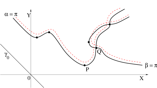
Figure 4: The level sets $\{\alpha=\pi\}$ and $\{\beta=\pi\}$ in a solution with generic singularities. In the $X$-$Y$ plane these are smooth curves which are structurally stable w.r.t. small ${\mathcal{C}}^{2}$ perturbations.

Throughout the following, we shall be interested not in a single solution but in a continuous path of solutions $\theta\mapsto u^{\theta}$, $\theta\in[0,1]$. We introduce suitable regularity conditions, allowing us to compute the “length” of this path by integrating a suitable norm of its tangent vector $\|du^{\theta}(t,\cdot)/d\theta\|$. Definition 1. We say that a solution $u=u(t,x)$ of (2.1) has generic singularities for $t\in[0,T]$ if it admits a representation of the form (5.23), where (i) the functions $(u,\alpha,\beta,p,q,x,t)(X,Y)$ are ${\mathcal{C}}^{\infty}$, and (ii) on the domain where $t(X,Y)\in[0,T]$ the following generic conditions hold:

• $\alpha=\pi$,  $\alpha_{X}=0\qquad\Longrightarrow\qquad\alpha_{Y}\not=0$,  $\alpha_{XX}\not=0$,

• $\beta=\pi$,  $\beta_{Y}=0\qquad\Longrightarrow\qquad\beta_{X}\not=0$,  $\beta_{YY}\not=0$,

• $\alpha=\pi$,  $\beta=\pi,\qquad\Longrightarrow\qquad\alpha_{X}\not=0$,  $\beta_{Y}\not=0$.

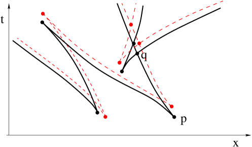
Figure 5: The set of singular points (where $|u_{x}|\to+\infty$) in a solution $u(t,x)$. These are the images of the sets $\{\alpha=\pi\}$ and $\{\beta=\pi\}$ in Fig. 4. By structural stability, every small perturbation will yield anther solution with the same type of singularities.

Some words of explanation are in order. Even if the solution $(X,Y)\mapsto(x,t,u,\alpha,\beta,p,q)(X,Y)$ of the semilinear system (5.11)–(5.15) remains smooth on the entire $X$-$Y$ plane, the function $u=u(t,x)$ in (5.23) can have singularities because the coordinate change $\Lambda:(X,Y)\mapsto(x,t)$ is not smoothly invertible. Indeed, by (5.15)-(5.14), the Jacobian matrix is computed by

$$D\Lambda~{}=~{}\left(\begin{array}[]{cc}x_{X}&x_{Y}\cr t_{X}&t_{Y}\end{array}\right)~{}=~{}\left(\begin{array}[]{ccc}{(1+\cos\alpha)\,p\over 4}&&-{(1+\cos\beta)\,q\over 4}\\[8.53581pt] {(1+\cos\alpha)\,p\over 4c(u)}&&{(1+\cos\beta)\,q\over 4c(u)}\end{array}\right)$$ (5.24)

We recall that $p,q$ remain uniformly positive and uniformly bounded on compact subsets of the $X$-$Y$ plane. By Remark 3, at a point $(X_{0},Y_{0})$ where $\alpha\not=\pi$ and $\beta\not=\pi$, this matrix is invertible, having a strictly positive determinant. The function $u=u(x,t)$ considered at (5.23) is thus smooth on a neighborhood of the point

$$(t_{0},x_{0})~{}=~{}\bigl{(}t(X_{0},Y_{0})\,,~{}x(X_{0},Y_{0})\Bigr{)}.$$

To study the set of points in the $x$-$t$ plane where $u$ is singular, we thus need to look at points where either $w=\pi$ or $\beta=\pi$. The generic conditions (G1)–(G2) guarantee that these level sets are smooth curves in the $X$-$Y$ plane. Condition (G3) implies that the level sets where $\{\alpha=\pi\}$ and $\{\beta=\pi\}$ intersect transversally because $\alpha_{Y}=\beta_{X}=0$ when $\alpha=\beta=0$. As observed in [7], the conditions (G1)–(G3) are invariant w.r.t. smooth variable transformations $(X,Y)\leftrightarrow(\widetilde{X},\widetilde{Y})$. We also remark that, if a solution $U=(u,\alpha,\beta,p,q)$ of (5.11)–(5.13) satisfies the generic conditions (G1)–(G3), then by the implicit function theorem the same is true for every perturbed solution $\widetilde{U}=(\tilde{u},\tilde{\alpha},\tilde{\beta},\tilde{p},\tilde{q})$ sufficiently close to $U$. In other words, generic singularities are structurally stable. An example of structurally unstable solution, corresponding to a change of topology in the singular set, is shown in Fig. 6. Definition 2. We say that a path of initial data $\gamma:\theta\mapsto(u_{0}^{\theta},u_{1}^{\theta})$, $\theta\in[0,1]$ is a piecewise regular path if the following conditions are satisfied.

• There exists a continuous map $(X,Y,\theta)\mapsto(u,\alpha,\beta,p,q,x,t)$ such that, for each $\theta\in[0,1]$ the semilinear system (5.11)–(5.15) is satisfied. Moreover, the function $u^{\theta}(x,t)$ whose graph is

  $$\hbox{Graph}(u^{\theta})~{}=~{}\Big{\{}(t,x,u)(X,Y,\theta);~{}~{}(X,Y)\in{\mathbb{R}}^{2}\Big{\}}$$ (5.25)

  provides the conservative solution of (1.1) with initial data

  $$u^{\theta}(0,x)~{}=~{}u^{\theta}_{0}(x)\,,\qquad\qquad u^{\theta}_{t}(0,x)~{}=~{}u^{\theta}_{1}(x)\,.$$

• There exist finitely many values $0=\theta_{0}<\theta_{1}<\cdots<\theta_{N}=1$ such that the following holds. For $\theta\in\,]\theta_{i-1},\theta_{i}[$, the map $(X,Y,\theta)\mapsto(u,\alpha,\beta,p,q,x,t)$ is ${\mathcal{C}}^{\infty}$. Moreover, the solution $u^{\theta}=u^{\theta}(t,x)$ has generic singularities at time $t=0$.

In addition, if for all $\theta\in[0,1]\setminus\{\theta_{1},\ldots,\theta_{N}\}$, the solution $u^{\theta}$ has generic singularities for $t\in[0,T]$, then we say that the path of solutions $\gamma:\theta\mapsto u^{\theta}$ is piecewise regular for $t\in[0,T]$. Remark 6. According to Remark 3, there are infinitely many parameterizations of the variables $(X,Y)$ that yield the same solution $u=u(t,x)$. However, as shown in [7], the property of having generic singularities is independent of the particular representation used in (5.25). Remark 7. The above definition has a simple motivation. If $\gamma$ is a piecewise regular path, then we can compute its length as an integral of the norm of a tangent vector. In addition, if $\gamma$ is piecewise regular for $t\in[0,T]$, then the length of the path of solutions $\gamma^{t}:\theta\mapsto(u^{\theta}(t,\cdot),u_{t}^{\theta}(t,\cdot))$ is well defined not only at $t=0$ but for all $t\in[0,T]$. See Definition 3 in Section 6 for details. Remark 8. In Definition 2, the finitely many values of $\theta$ where $u^{\theta}$ does not have structurally stable singularities correspond to bifurcation values. As $\theta$ crosses one of these values, the topological structure of the singular set (where $u^{\theta}_{x}\to\pm\infty$) usually changes, as shown in Fig. 6.

Figure 6: Here the solution $u^{\theta}$ has generic (i.e., structurally stable) singularities for $\theta<\bar{\theta}$ and for $\theta>\bar{\theta}$. However, when the parameter $\theta$ crosses the critical value $\bar{\theta}$, the topology of the singular set changes.

Following [7], on the wave speed $c$ we assume

• The map $c:{\mathbb{R}}\mapsto{\mathbb{R}}_{+}$ is smooth and uniformly positive. The quotient $c^{\prime}(u)/c(u)$ is uniformly bounded. Moreover, the following generic condition is satisfied:

  $$c^{\prime}(u)~{}=~{}0\qquad\Longrightarrow\qquad c^{\prime\prime}(u)~{}\not=~{}0.$$ (5.26)

Notice that, by (5.26), the derivative $c^{\prime}(u)$ vanishes only at isolated points. The following result, proved in [7], shows that the set of piecewise regular paths is dense. Theorem 4. Let the wave speed $c(u)$ satisfy the assumptions (A) and let $T>0$ be given. Let $\theta\mapsto(t^{\theta},x^{\theta},u^{\theta},\alpha^{\theta},\beta^{\theta},p^{\theta},q^{\theta})$, $\theta\in[0,1]$, be a smooth path of solutions to (5.11)–(5.15). Then there exists a sequence of paths of solutions $\theta\mapsto(t^{\theta}_{n},x^{\theta}_{n},u^{\theta}_{n},\alpha^{\theta}_{n},\beta^{\theta}_{n},p^{\theta}_{n},q^{\theta}_{n})$ with the following properties.

• For each $n\geq 1$, the path of corresponding solutions of (2.1) $\theta\mapsto u^{\theta}_{n}$ is regular for $t\in[0,T]$, according to Definition 2.

• For any bounded domain $\Omega$ in the $X$-$Y$ plane, as $n\to\infty$ the functions $(t^{\theta}_{n},x^{\theta}_{n},u^{\theta}_{n},\alpha^{\theta}_{n},\beta^{\theta}_{n},$ $p^{\theta}_{n},q^{\theta}_{n})$ converge to $(t^{\theta},x^{\theta},u^{\theta},\alpha^{\theta},\beta^{\theta},p^{\theta},q^{\theta})$ uniformly in ${\mathcal{C}}^{k}([0,1]\times\Omega)$, for every $k\geq 1$.

Thanks to this density result, to construct a Lipschitz metric it now remains to show that the weighted length of a regular path satisfies the same estimates as the smooth paths considered in the previous section. Toward this goal, we first derive an expression for the norm of a tangent vector as a line integral in the $X$-$Y$ coordinates.

Consider a reference solution $u$ (2.1) and a family of perturbed solutions $u^{\varepsilon}$, $\varepsilon\in[0,\varepsilon_{0}]$. We assume that, in the $X$-$Y$ coordinates, these define a smooth family of solutions of (5.11)–(5.15), say $(t^{\varepsilon},x^{\varepsilon},u^{\varepsilon},\alpha^{\varepsilon},\beta^{\varepsilon},p^{\varepsilon},q^{\varepsilon})$. For each $\varepsilon$, the curves where $X$ =constant and $Y$ = constant correspond respectively to backward and forward characteristics of the solutions $u^{\varepsilon}(t,x)$. We remark that, at time $t=0$, we have considerable freedom in choosing these parameterizations. We can take advantage of this in the following way. Let $w,z$ be the shifts in (3.26). At time $t=0$ we choose the parameterizations according to

$$X^{\varepsilon}(0,~{}x+\varepsilon\,w(0,x))~{}=~{}x\,,\qquad\qquad Y^{\varepsilon}(0,~{}x+\varepsilon\,z(0,x))~{}=~{}-x\,.$$ (5.27)

Consider the curve in $X$-$Y$ space

$$\Gamma_{\tau}~{}=~{}\{(X,Y)\,,~{}t(X,Y)=\tau\}~{}=~{}\{(X,Y(\tau,X))\,;~{}~{}X\in{\mathbb{R}}\}~{}=~{}\{(X(\tau,Y),\,Y)\,;~{}~{}Y\in{\mathbb{R}}\}\,,$$ (5.28)

and denote by

$$\Gamma^{\varepsilon}_{\tau}~{}=~{}\{(X,Y)\,,~{}t^{\varepsilon}(X,Y)=\tau\}~{}=~{}\{(X,Y^{\varepsilon}(\tau,X))\,;~{}~{}X\in{\mathbb{R}}\}~{}=~{}\{(X^{\varepsilon}(\tau,Y),\,Y)\,;~{}~{}Y\in{\mathbb{R}}\}$$ (5.29)

the perturbed curve. We can write the perturbed solutions as

$$(t^{\varepsilon},x^{\varepsilon},u^{\varepsilon},\alpha^{\varepsilon},\beta^{\varepsilon},p^{\varepsilon},q^{\varepsilon})~{}=~{}(t,x,u,\alpha,\beta,p,q)+\varepsilon({\mathcal{T}},{\mathcal{X}},U,A,B,P,Q)+o(\varepsilon)$$ (5.30)

Since the system (5.15)–(5.11) has smooth coefficients, the first order perturbations satisfy a linearized system and are well defined for all $(X,Y)\in{\mathbb{R}}^{2}$. We observe that the quantities $v,\tilde{r},\tilde{s},w,z$ appearing in (3.15) can be expressed in terms of the first order perturbations $({\mathcal{T}},{\mathcal{X}},U,A,B,P,Q)$. Indeed,

$$(1+R^{2})\,dx~{}=~{}p\,dX\,,\qquad\qquad(1+S^{2})\,dx~{}=~{}-q\,dY$$

Notice that, by definition,

$$t^{\varepsilon}(X,\,Y^{\varepsilon}(\tau,X))~{}=~{}t^{\varepsilon}(X^{\varepsilon}(\tau,Y),Y)~{}=~{}\tau.$$

Hence by the implicit function theorem, at $\varepsilon=0$:

$${\partial X^{\varepsilon}\over\partial\varepsilon}~{}=~{}-{\partial t^{\varepsilon}\over\partial\varepsilon}\cdot\left({\partial t\over\partial X}\right)^{-1}~{}=~{}-{\mathcal{T}}\frac{4c}{(1+\cos\alpha)p}$$

and

$${\partial Y^{\varepsilon}\over\partial\varepsilon}~{}=~{}-{\partial t^{\varepsilon}\over\partial\varepsilon}\cdot\left({\partial t\over\partial Y}\right)^{-1}~{}=~{}-{\mathcal{T}}\frac{4c}{(1+\cos\beta)q}\,.$$

1.

The shift in $x$ is computed by

$$\left.\begin{array}[]{rcl}w&=&\lim_{\varepsilon\to 0}~{}{x^{\varepsilon}(X,Y^{\varepsilon}(\tau,X))-x(X,Y(\tau,X))\over\varepsilon}\\[5.69054pt] &=&{\mathcal{X}}(X,Y(\tau,X))+x_{Y}\cdot{\partial Y^{\varepsilon}\over\partial\varepsilon}\Big{|}_{\varepsilon=0}~{}=~{}({\mathcal{X}}+c{\mathcal{T}})(X,Y(\tau,X)).\end{array}\right.$$

In a similar way,

$$\left.\begin{array}[]{rcl}z&=&\lim_{\varepsilon\to 0}~{}{x^{\varepsilon}(X^{\varepsilon}(\tau,Y),Y)-x(X(\tau,Y),Y)\over\varepsilon}\\[5.69054pt] &=&{\mathcal{X}}(X(\tau,Y),Y)+x_{X}\cdot{\partial X^{\varepsilon}\over\partial\varepsilon}\Big{|}_{\varepsilon=0}~{}=~{}({\mathcal{X}}-c{\mathcal{T}})(X(\tau,Y),Y),\end{array}\right.$$

2.

We now derive an expression for $\tilde{r},\tilde{s}$. One has

$$r+wR_{x}~{}=~{}{d\over d\varepsilon}\tan{\alpha^{\varepsilon}(X,Y^{\varepsilon}(\tau,X))\over 2}\Big{|}_{\varepsilon=0}~{}=~{}\frac{1}{2}\Big{(}A-{\mathcal{T}}\frac{4c}{(1+\cos\beta)q}\alpha_{Y}\Big{)}\sec^{2}\frac{\alpha}{2}$$ (5.31)

and

$$s+zS_{x}~{}=~{}{d\over d\varepsilon}\tan{\beta^{\varepsilon}(X^{\varepsilon}(\tau,Y),Y)\over 2}\Big{|}_{\varepsilon=0}~{}=~{}\frac{1}{2}\Big{(}B-{\mathcal{T}}\frac{4c}{(1+\cos\alpha)p}\beta_{X}\Big{)}\sec^{2}\frac{\beta}{2}\,.$$ (5.32)

By (3.14) it thus follows

$$\tilde{r}~{}=~{}\frac{1}{2}\Big{(}A-{\mathcal{T}}\frac{4c}{(1+\cos\beta)q}\alpha_{Y}\Big{)}\sec^{2}\frac{\alpha}{2}-\frac{c^{\prime}}{4c}{\mathcal{T}}\tan^{2}\frac{\beta}{2}$$ (5.33)

and

$$\tilde{s}~{}=~{}\frac{1}{2}\Big{(}B-{\mathcal{T}}\frac{4c}{(1+\cos\alpha)p}\beta_{X}\Big{)}\sec^{2}\frac{\beta}{2}-\frac{c^{\prime}}{4c}{\mathcal{T}}\tan^{2}\frac{\alpha}{2}\,.$$ (5.34)

3.

By (5.11) one has

$$v+u_{x}w~{}=~{}{d\over d\varepsilon}u^{\varepsilon}(X,Y^{\varepsilon}(\tau,X))\Big{|}_{\varepsilon=0}~{}=~{}U-u_{Y}{\mathcal{T}}\frac{4c}{(1+\cos\beta)q}~{}=~{}U-{\mathcal{T}}\tan\frac{\alpha}{2}\,.$$

Therefore

$$v+\frac{Rw}{2c}-\frac{Sz}{2c}~{}=~{}U-(\tan\frac{\alpha}{2}+\tan\frac{\beta}{2})\cdot{\mathcal{T}}\,.$$ (5.35)

4.

We now calculate the terms $I_{4}$ – $I_{6}$ in (3.15).

The change in base measure with density $1+R^{2}$ is given by

$$\lim_{\varepsilon\to 0}~{}{p^{\varepsilon}(X,Y^{\varepsilon}(\tau,X))-p(X,Y(\tau,X))\over\varepsilon}~{}=~{}P(X,Y)+p_{Y}\cdot{\partial Y^{\varepsilon}\over\partial\varepsilon}\Big{|}_{\varepsilon=0}~{}=~{}P-{\mathcal{T}}\frac{4c}{(1+\cos\beta)q}p_{Y}\,.$$ (5.36)

The change in base measure with density $1+S^{2}$ is given by

$$\lim_{\varepsilon\to 0}~{}{q^{\varepsilon}(X^{\varepsilon}(\tau,Y),Y)-q(X(\tau,Y),Y)\over\varepsilon}~{}=~{}Q(X,Y)+q_{X}\cdot{\partial X^{\varepsilon}\over\partial\varepsilon}\Big{|}_{\varepsilon=0}~{}=~{}Q-{\mathcal{T}}\frac{4c}{(1+\cos\alpha)p}q_{X}\,.$$ (5.37)

The change in base measure with density $R^{2}$ (the integrand in $I_{6}$) is estimated by

$$\left.\begin{array}[]{l}\displaystyle{d\over d\varepsilon}\Big{(}p^{\varepsilon}\sin^{2}\frac{\alpha^{\varepsilon}}{2}(X,Y^{\varepsilon}(\tau,X))\Big{)}\Big{|}_{\varepsilon=0}\\[11.38109pt] \displaystyle\qquad=~{}\Big{(}P-{\mathcal{T}}\frac{4c}{(1+\cos\beta)q}p_{Y}\Big{)}\sin^{2}\frac{\alpha}{2}~{}+~{}\frac{p\sin\alpha}{2}\Big{(}A-{\mathcal{T}}\frac{4c}{(1+\cos\beta)q}\alpha_{Y}\Big{)}\,.\end{array}\right.$$ (5.38)

The difference between (5.36) and (5.38) shows that the change in base measure with density 1 (the integrand in $I_{4}$) is computed by

$$\Big{(}P-{\mathcal{T}}\frac{4c}{(1+\cos\beta)q}p_{Y}\Big{)}\cos^{2}\frac{\alpha}{2}~{}-~{}\frac{p\sin\alpha}{2}\Big{(}A-{\mathcal{T}}\frac{4c}{(1+\cos\beta)q}\alpha_{Y}\Big{)}\,.$$ (5.39)

Combining the previous computations, the weighted norm of a tangent vector (3.15) can be written as a line integral over the line $\Gamma_{\tau}$ defined at (5.28):

$$\Big{\|}(\tilde{r},w,\tilde{s},z)\Big{\|}_{(u,R,S)}~{}=~{}\sum_{\ell=1}^{6}\kappa_{\ell}\cdot\int_{\Gamma_{\tau}}\Big{\{}|J_{\ell}|\,{\mathcal{W}}^{-}\,dX+|H_{\ell}|\,{\mathcal{W}}^{+}\,dY\Big{\}}\,,$$ (5.40)

where

$$\begin{array}[]{rcl}J_{1}&=&({\mathcal{X}}-c{\mathcal{T}})p\\[11.38109pt] J_{2}&=&\frac{1}{2}\Big{(}Ap-{\mathcal{T}}\frac{4cp}{(1+\cos\beta)q}\alpha_{Y}\Big{)}-\frac{c^{\prime}}{4c}p{\mathcal{T}}\tan^{2}\frac{\beta}{2}\cos^{2}\frac{\alpha}{2}\\[11.38109pt] J_{3}&=&\Big{(}U-(\tan\frac{\alpha}{2}+\tan\frac{\beta}{2})\cdot{\mathcal{T}}\Big{)}p\\[11.38109pt] J_{4}&=&P\cos^{2}\frac{\alpha}{2}-{\mathcal{T}}\frac{2c}{q}p_{Y}\frac{\cos^{2}\frac{\alpha}{2}}{\cos^{2}\frac{\beta}{2}}-\frac{p\sin\alpha}{2}A+\frac{2cp}{q}\,{\mathcal{T}}\alpha_{Y}\frac{\sin\alpha}{1+\cos\beta}+\frac{c^{\prime}}{2c}p{\mathcal{T}}\tan\frac{\beta}{2}\cos^{2}\frac{\alpha}{2}\\[11.38109pt] J_{5}&=&J_{4}\cdot\tan\frac{\alpha}{2}\\[11.38109pt] &=&\frac{1}{2}P\sin\alpha-{\mathcal{T}}\frac{2c}{q}p_{Y}\frac{\sin\frac{\alpha}{2}\cos\frac{\alpha}{2}}{\cos^{2}\frac{\beta}{2}}-pA\sin^{2}\frac{\alpha}{2}+\frac{2cp}{q}\,{\mathcal{T}}\alpha_{Y}\frac{\sin^{2}\frac{\alpha}{2}}{\cos^{2}\frac{\beta}{2}}+\frac{c^{\prime}}{4c}p{\mathcal{T}}\tan\frac{\beta}{2}\sin{\alpha}\\[11.38109pt] J_{6}&=&\Big{(}P-{\mathcal{T}}\frac{4c}{(1+\cos\beta)q}p_{Y}\Big{)}\sin^{2}\frac{\alpha}{2}+\frac{p\sin\alpha}{2}A-\frac{2cp}{q}\,{\mathcal{T}}\alpha_{Y}\frac{\sin\alpha}{1+\cos\beta}\\[11.38109pt] &&\qquad+\frac{c^{\prime}}{2c}(\sin^{2}\frac{\alpha}{2}\tan\frac{\beta}{2}-\tan^{2}\frac{\beta}{2}\sin\frac{\alpha}{2}\cos\frac{\alpha}{2}){\mathcal{T}}p\,.\end{array}$$

Using (5.13) and (5.12), the above expression can be simplified as

$$\left\{\begin{array}[]{rcl}J_{1}&=&({\mathcal{X}}-c{\mathcal{T}})p\\[11.38109pt] J_{2}&=&\frac{1}{2}Ap-\frac{c^{\prime}}{4c}p{\mathcal{T}}\sin^{2}\frac{\alpha}{2}\\[11.38109pt] J_{3}&=&\Big{(}U-(\tan\frac{\alpha}{2}+\tan\frac{\beta}{2})\cdot{\mathcal{T}}\Big{)}p\\[11.38109pt] J_{4}&=&P\cos^{2}\frac{\alpha}{2}-\frac{p\sin\alpha}{2}A+\frac{c^{\prime}}{4c}{\mathcal{T}}p\sin\alpha\\[11.38109pt] J_{5}&=&\frac{1}{2}P\sin\alpha-pA\sin^{2}\frac{\alpha}{2}+\frac{c^{\prime}}{2c}{\mathcal{T}}p\sin^{2}\frac{\alpha}{2}\\[11.38109pt] J_{6}&=&P\sin^{2}\frac{\alpha}{2}+\frac{p\sin\alpha}{2}A\,.\end{array}\right.$$ (5.41)

In a similar way, we obtain

$$\left\{\begin{array}[]{rcl}H_{1}&=&({\mathcal{X}}+c{\mathcal{T}})q\\[11.38109pt] H_{2}&=&\frac{1}{2}Bq-\frac{c^{\prime}}{4c}q{\mathcal{T}}\sin^{2}\frac{\beta}{2}\\[11.38109pt] H_{3}&=&\Big{(}U-(\tan\frac{\alpha}{2}+\tan\frac{\beta}{2})\cdot{\mathcal{T}}\Big{)}q\\[11.38109pt] H_{4}&=&Q\cos^{2}\frac{\beta}{2}-\frac{q\sin\beta}{2}B+\frac{c^{\prime}}{4c}{\mathcal{T}}q\sin\beta\\[11.38109pt] H_{5}&=&\frac{1}{2}Q\sin\beta-qB\sin^{2}\frac{\beta}{2}+\frac{c^{\prime}}{2c}{\mathcal{T}}q\sin^{2}\frac{\beta}{2}\\[11.38109pt] H_{6}&=&Q\sin^{2}\frac{\beta}{2}+\frac{q\sin\beta}{2}B\end{array}\right.$$ (5.42)

It is clear that the integrands $J_{\ell}$, $H_{\ell}$ are smooth, for $\ell=1,2,4,5,6$. We claim that the integrands $J_{3}$ and $H_{3}$ are continuous as well. Indeed, using (5.35) we obtain

$$\begin{array}[]{l}U-(\tan\frac{\alpha}{2}+\tan\frac{\beta}{2})\cdot{\mathcal{T}}\\[11.38109pt] \qquad=~{}2cv+Rw-Sz\\[11.38109pt] \qquad=~{}\int\left(\frac{c^{\prime}}{c}(R-S)v+2cv_{x}+wR_{x}+Rw_{x}-zS_{x}-Sz_{x}\right)~{}dx\\[11.38109pt] \qquad=~{}\int\Big{(}r-s+wR_{x}+Rw_{x}-zS_{x}-Sz_{x}\Big{)}\,dx\\[11.38109pt] \qquad=~{}\int\Big{(}r+Rw_{x}-\frac{c^{\prime}}{8c^{2}}(w-z)S^{2}\Big{)}\,dx-\int\Big{(}s+zS_{x}-\frac{c^{\prime}}{8c^{2}}(w-z)R^{2})\Big{)}\,dx\\[11.38109pt] \quad\qquad+\int\Big{(}wR_{x}+\frac{c^{\prime}}{4c^{2}}R^{2}S(w-z)\Big{)}\,dx-\int\Big{(}Sz_{x}+\frac{c^{\prime}}{4c^{2}}R^{2}S(w-z)\Big{)}\,dx\\[11.38109pt] \qquad\quad+\int\Big{(}\frac{c^{\prime}}{8c^{2}}(w-z)(S^{2}-R^{2})\Big{)}\,dx\,.\end{array}$$

The three terms on the right hand side correspond to the integrands in $I_{2}$, $I_{4}$ and $I_{1}$, respectively. Hence they are continuous.

6 Length of piecewise regular paths

Let $\gamma:\theta\mapsto(u_{0}^{\theta},u_{1}^{\theta})$ be a piecewise regular path of initial data. According to Definition 2. there exists a smooth path of solutions of (5.11)–(5.15), say $\theta\mapsto(x^{\theta},t^{\theta},u^{\theta},\alpha^{\theta},\beta^{\theta},p^{\theta},q^{\theta})(X,Y)$, such that (5.25) holds for every $\theta\in[0,1]$. At time $t=0$, an upper bound on the length of this path can be computed as follows. For each $\theta\in[0,1]$, consider the curve in the $X$-$Y$ plane

$$\Gamma^{\theta}_{0}~{}\doteq~{}\Big{\{}(X,Y)\,;~{}~{}t^{\theta}(X,Y)=0\Big{\}}.$$

The norm of the tangent vector is then determined by (5.40). Integrating w.r.t. $\theta$ we obtain

$$\int_{0}^{1}\left(\sum_{\ell=1}^{6}\kappa_{\ell}\cdot\int_{\Gamma_{0}^{\theta}}\Big{\{}|J_{\ell}^{\theta}|\,{\mathcal{W}}^{-}dX~{}+|H_{\ell}^{\theta}|\,{\mathcal{W}}^{+}\,dY\Big{\}}\right)\,d\theta\,.$$ (6.1)

We recall that there exist infinitely many paths of solutions of (5.11)–(5.15) which yields the same path of solutions to (2.1). Indeed, as shown in Remark 3, at time $t=0$ for each $\theta$ one can choose smooth, increasing functions $\phi^{\theta},\psi^{\theta}$ (smoothly depending on $\theta$), and define the solutions $(\tilde{x}^{\theta},\tilde{t}^{\theta},\tilde{u}^{\theta},\tilde{\alpha}^{\theta},\tilde{\beta}^{\theta},\tilde{p}^{\theta},\tilde{q}^{\theta})(\widetilde{X},\widetilde{Y})$ as in (5.18)–(5.20).

On the other hand, different relabelings of the $X,Y$ coordinates determine different values for the integral in (6.1). Indeed, these correspond to different choices of the shifts $w,z$ in (3.13). To illustrate this point more clearly, fix a value of $\theta$. Then, for $\varepsilon>0$ small, the family of solutions $u^{\theta+\varepsilon}$ can be regarded as perturbations of the solution $u^{\theta}$. At a given point $(\tau,\bar{x})$, the shifts $w(\tau,\bar{x})$ and $z(\tau,\bar{x})$ are uniquely determined as follows (Fig. 7). Let $X_{0},Y_{0}$ be the point in the $X$-$Y$ plane such that $x^{\theta}(X_{0},Y_{0})=\bar{x}$, $t^{\theta}(X_{0},Y_{0})=\tau$. For each $\varepsilon>0$, define $X^{\varepsilon}$ and $Y^{\varepsilon}$ implicitly by setting

$$t^{\theta+\varepsilon}(X_{0},Y_{\varepsilon})~{}=~{}\tau\,,\qquad\qquad t^{\theta+\varepsilon}(X_{\varepsilon},Y_{0})~{}=~{}\tau\,.$$

The shifts are then uniquely defined by setting

$$w(\tau,\bar{x},)~{}=~{}\lim_{\varepsilon\to 0}~{}{x^{\theta+\varepsilon}(X_{0},Y_{\varepsilon})-x^{\theta}(X_{0},Y_{0})\over\varepsilon}\,,\qquad z(\tau,\bar{x})~{}=~{}\lim_{\varepsilon\to 0}~{}{x^{\theta+\varepsilon}(X_{\varepsilon},Y_{0})-x^{\theta}(X_{0},Y_{0})\over\varepsilon}\,.$$ (6.2)

Figure 7: Given a representation of the solutions $u^{\theta}$ in terms of the variables $X,Y$, the shifts $w,z$ are uniquely determined by (6.2). Here $\Gamma_{\tau}^{\theta}=\{(X,Y)\,;~{}~{}t^{\theta}(X,Y)=\tau\}$.

The above considerations lead to Definition 3. The length $\|\gamma\|$ of the piecewise regular path $\gamma:\theta\mapsto(u_{0}^{\theta},u_{1}^{\theta})$ is defined as the infimum of the expressions in (6.1), taken over all piecewise smooth relabelings of the $X$-$Y$ coordinates. Based on the analysis in Section 3, we now give an estimate on how the length of a regular path can grow in time. Theorem 5. Given any $K,T>0$, there exist constants $\kappa_{1},\ldots,\kappa_{6}$ in (6.1) and $C_{K,T}>0$ such that the following holds. Consider a path of solutions $\theta\mapsto(u^{\theta},u_{t}^{\theta})$ of (1.1), which is piecewise regular for $t\in[0,T]$ and where each $u^{\theta}$ has total energy $\leq K$. Then its length satisfies the estimates

$$\|\gamma^{\tau}\|~{}\leq~{}C_{K,T}\,\|\gamma^{0}\|\qquad\qquad\hbox{for all}~{}~{}0\leq\tau\leq T\,.$$ (6.3)

Proof. 1. To fix the ideas, let $u^{\theta}$ be structurally stable for every $\theta\in[0,1]\setminus\{\theta_{1},\ldots,\theta_{N}\}$.

Fix $\varepsilon>0$ and choose a relabeling of the variables $X,Y$ such that, at time $t=0$,

$$\int_{0}^{1}\left(\sum_{\ell=1}^{6}\kappa_{\ell}\cdot\int_{\Gamma_{0}^{\theta}}\Big{\{}|J_{\ell}^{\theta}|\,{\mathcal{W}}^{-}dX~{}+|H_{\ell}^{\theta}|\,{\mathcal{W}}^{+}\,dY\Big{\}}\right)\,d\theta~{}\leq~{}\|\gamma^{0}\|+\varepsilon\,.$$ (6.4)

Since the solution $u$ is smooth in the $X$-$Y$ variables and piecewise smooth in the $x$-$t$ variables, the existence of the tangent vector is clear, for every $\theta\in[0,1]$ and $t\in[0,T]$. We claim that, for every $\theta\notin\{\theta_{1},\ldots,\theta_{N}\}$, an estimate such as (3.22) holds. Namely

$$\begin{array}[]{l}\displaystyle\Big{\|}(v^{\theta}(\tau),r^{\theta}(\tau),s^{\theta}(\tau))\Big{\|}_{(u^{\theta}(\tau),R^{\theta}(\tau),S^{\theta}(\tau))}\cr\cr\qquad\displaystyle~{}\leq~{}\exp\left\{C_{0}\tau+\int_{0}^{\tau}a^{\theta}(s)ds\right\}\cdot\Big{\|}(v^{\theta}(0),r^{\theta}(0),s^{\theta}(0))\Big{\|}_{(u^{\theta}(0),R^{\theta}(0),S^{\theta}(0))}\,.\end{array}$$ (6.5)

Here the constant $C_{0}$ and the integral of $a^{\theta}$ depend only on $T$ and on an upper bound on the total energy.

Integrating (6.5) over the interval $\theta\in[0,1]$, one obtains an estimate of the form

$$\|\gamma^{\tau}\|~{}\leq~{}C\,\bigl{(}\|\gamma^{0}\|+\varepsilon\bigr{)}\qquad\qquad\hbox{for all}~{}~{}0\leq\tau\leq T\,.$$

This proves (6.3), because $\varepsilon>0$ was arbitrary. 2. It now remains to prove the estimate (6.5). We observe that, if $u^{\theta}$ were smooth for all $(x,t)\in{\mathbb{R}}\times[0,\tau]$, the result follows directly from (3.25), proved by the computations in Section 4. We need to show that the same conclusion can be reached if $u^{\theta}$ is piecewise smooth, with structurally stable singularities.

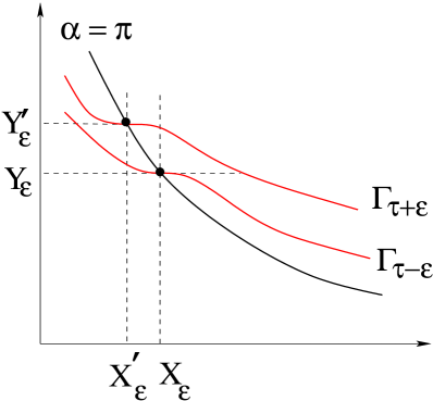
Figure 8: Proving that the rate of change in the length of a tangent vector is not affected by the presence of a singularity.

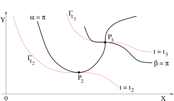
Figure 9: Here $P_{2}$ is a singularity point of Type 2, where $\alpha=\pi$ and $\alpha_{X}=0$, but $\alpha_{XX}\not=0$ and $\beta\not=\pi$. At $P_{3}$ the solution has a singularity of Type 3, where $\alpha=\beta=\pi$, but $\alpha_{X}\not=0$ and $\beta_{Y}\not=0$. The weighted norm of the tangent vector is continuous at the times $t=t_{2}$ and $t=t_{3}$.

Fix a time $\tau$ and call $\Gamma_{\tau}\doteq\{t^{\theta}(X,Y)=\tau\}$ the level set in the $X$-$Y$ plane. Since the estimates of the previous section hold in regions where $u^{\theta}$ is smooth, to obtain a bound on the weighted norm of the tangent vector it suffices to show that the effect of isolated singularities is negligible. To lighten the notation, in the following the superscript ^θ will be omitted.

With reference to Fig. 8, assume that the solution has a structurally stable singularity along a backward characteristic. We claim that this singularity does not affect the estimate (3.25). In other words, the time derivative

$${d\over dt}\sum_{\ell=1}^{6}\kappa_{\ell}\cdot\int_{\Gamma_{t}}\Big{\{}|J_{\ell}|\,{\mathcal{W}}^{-}\,dX+|H_{\ell}|\,{\mathcal{W}}^{+}\,dY\Big{\}}$$

is not affected by the presence of the singularity.

For a given time $\tau$, let $(X_{\varepsilon},Y_{\varepsilon})$ be the point where the curve $\Gamma_{\tau-\varepsilon}=\{t(X,Y)=\tau-\varepsilon\}$ intersects the singular curve $\{\alpha(X,Y)=\pi\}$. Similarly, let $(X^{\prime}_{\varepsilon},Y^{\prime}_{\varepsilon})$ be the point where the curve $\Gamma_{\tau+\varepsilon}=\{t(X,Y)=\tau+\varepsilon\}$ intersects the singular curve $\{\alpha(X,Y)=\pi\}$.

Define the curves

$$\left\{\begin{array}[]{rl}\sigma_{\varepsilon}^{+}&\doteq~{}\Gamma_{\tau+\varepsilon}\cap\{X\in[X_{\varepsilon}^{\prime},X_{\varepsilon}]\}\,,\cr\sigma_{\varepsilon}^{-}&\doteq~{}\Gamma_{\tau-\varepsilon}\cap\{x\in[X_{\varepsilon}^{\prime},X_{\varepsilon}]\}\,,\end{array}\right.\qquad\qquad\left\{\begin{array}[]{rl}\eta_{\varepsilon}^{+}&\doteq~{}\Gamma_{\tau+\varepsilon}\cap\{Y\in[Y_{\varepsilon},Y_{\varepsilon}]\}\,,\cr\eta_{\varepsilon}^{-}&\doteq~{}\Gamma_{\tau-\varepsilon}\cap\{Y\in[Y_{\varepsilon},Y_{\varepsilon}]\}\,.\end{array}\right.$$

To prove our claim, it suffices to show that

$$\lim_{\varepsilon\to 0}~{}{1\over\varepsilon}\left(\int_{\sigma_{\varepsilon}^{+}}-\int_{\sigma_{\varepsilon}^{-}}\right)\sum_{\ell=1}^{6}|J_{\ell}|{\mathcal{W}}^{-}\,dX~{}=~{}0\,,$$ (6.6)

$$\lim_{\varepsilon\to 0}~{}{1\over\varepsilon}\left(\int_{\eta_{\varepsilon}^{+}}-\int_{\eta_{\varepsilon}^{-}}\right)\sum_{\ell=1}^{6}|H_{\ell}|{\mathcal{W}}^{+}\,dY~{}=~{}0\,.$$ (6.7)

The first limit holds because the integrand is a continuous function of $X,Y$ and $|X_{\varepsilon}-X^{\prime}_{\varepsilon}|~{}=~{}{\cal O}(\varepsilon)$. The second limit holds because the integrand is a continuous function of $X,Y$ and $|Y_{\varepsilon}^{\prime}-Y_{\varepsilon}|~{}=~{}{\cal O}(\varepsilon)$. The basic estimate (3.25) thus remains valid also in the presence of singular curves where $\alpha=\pi$ or $\beta=\pi$. Finally, we analyze what happens in the presence of singular points of Type 2, where $\alpha=\pi$ and $\alpha_{x}=0$, and of Type 3, where $\alpha=\beta=\pi$. Since the solution $u^{\theta}$ is structurally stable, there can be at most finitely many such points, say

$$Q_{j}~{}=~{}(X_{j},Y_{j}),\qquad\qquad j=1,\ldots,N\,.$$

To complete the proof of our claim, it thus suffices to show that, at each time $\tau_{j}=t(X_{j},Y_{j})$, the map

$$t~{}\mapsto~{}\int_{0}^{1}\left(\sum_{\ell=1}^{6}\kappa_{\ell}\cdot\int_{\Gamma_{t}}\Big{\{}|J_{\ell}^{\theta}|\,{\mathcal{W}}^{-}dX~{}+|H_{\ell}^{\theta}|\,{\mathcal{W}}^{+}\,dY\Big{\}}\right)$$ (6.8)

is continuous at $t=\tau_{j}$. But this is clear, because the path $\Gamma_{t}$ depends continuously on $t$ and the integrands $J_{\ell},H_{\ell}$ are uniformly bounded. Moreover, they are continuous everywhere with a possible exception of the finitely many singular points $Q_{j}$. MM     

7 Construction of the geodesic distance

A key result proved in [7] shows that every path of solutions to (1.1) can be approximated by a path which remains regular for $t\in[0,T]$. More precisely, an application of Thom’s transversality theorem yields Theorem 6. Let the wave speed $c(u)$ satisfy the assumptions (A). Let $(u^{\theta},\alpha^{\theta},\beta^{\theta},p^{\theta},q^{\theta},x^{\theta},t^{\theta})(X,Y)$ be a path of ${\mathcal{C}}^{\infty}$ solutions to the semilinear system (5.11)–(5.15), depending smoothly on $\theta\in[0,1]$. Then, for any $T,\varepsilon>0$ and any integer $k\geq 1$, there exists a perturbed path of solutions $(\tilde{u}^{\theta},\tilde{\alpha}^{\theta},\tilde{\beta}^{\theta},\tilde{p}^{\theta},\tilde{q}^{\theta},\tilde{x}^{\theta},\tilde{t}^{\theta})(X,Y)$ such that

$$\Big{\|}(u^{\theta}-\tilde{u}^{\theta},~{}\alpha^{\theta}-\tilde{\alpha}^{\theta},~{}\beta^{\theta}-\tilde{\beta}^{\theta},~{}p^{\theta}-\tilde{p}^{\theta},~{}q^{\theta}-\tilde{q}^{\theta},~{}x^{\theta}-\tilde{x}^{\theta},~{}t^{\theta}-\tilde{t}^{\theta})\Big{\|}_{{\mathcal{C}}^{k}(\Omega)}~{}<~{}\varepsilon.$$ (7.1)

Here $\Omega\subset{\mathbb{R}}^{2}$ is a domain containing the set

$$\Big{\{}(X,Y)\,;~{}~{}t^{\theta}(X,Y)\in[0,T]~{}~{}\hbox{or}~{}~{}\tilde{t}^{\theta}(X,Y)\in[0,T]\,,\qquad\hbox{for some}~{}\theta\in[0,1]\Big{\}}.$$

Moreover, all except finitely many solutions $(\tilde{u}^{\theta},\tilde{\alpha}^{\theta},\tilde{\beta}^{\theta},\tilde{p}^{\theta},\tilde{q}^{\theta},\tilde{x}^{\theta},\tilde{t}^{\theta})$ have structurally stable singularities inside $\Omega$.

In other words, by slightly perturbing the initial data $(u_{0}^{\theta},u^{\theta}_{1})$, $\theta\in[0,1]$, we can construct a one-parameter family of conservative solutions $u^{\theta}=u^{\theta}(t,x)$ which have structurally stable singularities, for all but finitely many values of $\theta$. This implies that for all $t\in[0,T]$ the length of the path $\theta\mapsto u^{\theta}(t,\cdot)$ is well defined by the formula

$$\|\gamma^{t}\|~{}\doteq~{}\int_{0}^{1}\left\|{d\over d\theta}u^{\theta}(t)\right\|_{u^{\theta}(t)}\,d\theta\,.$$ (7.2)

Here $\|\cdot\|_{u}$ is a weighted norm defined as in (3.13)–(3.15), or equivalently at (5.40).

A geodesic distance $d^{*}$ on the space $H^{1}({\mathbb{R}})\times{\bf L}^{2}({\mathbb{R}})$ will be constructed in two steps.

• As proved in [7], there is an open dense set of initial data

  $${\mathcal{D}}~{}\subset~{}\Big{(}{\mathcal{C}}^{3}({\mathbb{R}})\cap H^{1}({\mathbb{R}})\Big{)}\times\Big{(}{\mathcal{C}}^{2}({\mathbb{R}})\cap{\bf L}^{2}({\mathbb{R}})\Big{)},$$ (7.3)

  such that, if $(u_{0},u_{1})\in{\mathcal{D}}$, then the solution of (2.1)-(2.2) has structurally stable singularities. On ${\mathcal{D}}^{\infty}\doteq{\mathcal{C}}^{\infty}_{c}\cap{\mathcal{D}}$ we construct a geodesic distance, defined as the infimum among the weighted lengths of all piecewise regular paths connecting two given points.

• By continuity, this distance can then be extended from ${\mathcal{D}}^{\infty}$ to a larger space, defined as the completion of ${\mathcal{D}}^{\infty}$ w.r.t. the distance $d^{*}$. In particular, this completion will contain the space $(H^{1}\cap W^{1,1})\times({\bf L}^{2}\cap{\bf L}^{1})$.

More in detail, assume $(u_{0},u_{1})$, $(\tilde{u}_{0},\tilde{u}_{1})\in{\mathcal{D}}^{\infty}$. Their total energies will be denoted by

$${\mathcal{E}}(u_{0},u_{1})~{}\doteq~{}\int\bigl{[}u_{1}^{2}+c^{2}(u_{0})u_{0,x}^{2}\bigr{]}\,dx\,,\qquad\qquad{\mathcal{E}}(\tilde{u}_{0},\tilde{u}_{1})~{}\doteq~{}\int\bigl{[}\tilde{u}_{1}^{2}+c^{2}(\tilde{u}_{0})\tilde{u}_{0,x}^{2}\bigr{]}\,dx\,,$$

respectively. Fix any constant $K>0$ and consider the subset of all data with energy $\leq K$, namely

$$X_{K}~{}\doteq~{}\Big{\{}(u_{0},u_{1})\in H^{1}({\mathbb{R}})\times{\bf L}^{2}({\mathbb{R}})\,;\quad{\mathcal{E}}(u_{0},u_{1})\leq K\Big{\}}\,.$$ (7.4)

Notice that $X_{K}$ is positively invariant for the flow generated by the wave equation. Definition 4. On ${\mathcal{D}}^{\infty}\cap X_{K}$ we define the geodesic distance $d^{*}\bigl{(}(u_{0},u_{1}),~{}(\tilde{u}_{0},\tilde{u}_{1})\bigr{)}$ as the infimum among all weighted lengths of piecewise regular paths, which connect $(u_{0},u_{1})$ with $(\tilde{u}_{0},\tilde{u}_{1})$, always remaining inside $X_{K}$. Namely,

$$\begin{array}[]{l}\displaystyle d^{*}\bigl{(}(u_{0},u_{1}),~{}(\tilde{u}_{0},\tilde{u}_{1})\bigr{)}~{}\doteq~{}\inf~{}\Big{\{}\|\gamma\|\,;~{}~{}\gamma~{}\hbox{is a piecewise regular path}\,,\cr\cr\qquad\qquad\gamma(0)=(u_{0},u_{1})\,,\quad\gamma(1)=(\tilde{u}_{0},\tilde{u}_{1})\qquad{\mathcal{E}}(u_{0}^{\theta},u_{1}^{\theta})\leq K\quad\hbox{for all}~{}\theta\in[0,1]\Big{\}}.\end{array}$$ (7.5)

Since the concatenation of two piecewise regular paths is still a piecewise regular path (after a suitable re-parameterization), it is clear that $d^{*}(\cdot,\cdot)$ is indeed a distance. As a consequence of Theorem 5, we have Theorem 7. Let the wave speed $c(\cdot)$ be smooth and satisfy (2.3). Then the geodesic distance $d^{*}$ renders Lipschitz continuous the flow generated by the wave equation (2.1). In particular, let $(u_{0},u_{1})$ and $(\tilde{u}_{0},\tilde{u}_{1})$ be two initial data in (2.2). Then for all $t\in[0,T]$ the corresponding solutions satisfy

$$d^{*}\Big{(}\bigl{(}u(t,\cdot),\,u_{t}(t,\cdot)\bigr{)},~{}\bigl{(}\tilde{u}(t,\cdot),\,\tilde{u}_{t}(t,\cdot)\bigr{)}\Big{)}~{}\leq~{}C_{K,T}\cdot d^{*}\Big{(}(u_{0},u_{1}),\,(\tilde{u}_{0},\tilde{u}_{1})\Big{)}\,.$$ (7.6)

Here $C_{K,T}$ is a constant depending only on $T$ and on an upper bound $K$ on the total energy. Proof. If the wave speed $c(\cdot)$ satisfies the generic assumption ${\bf(A)}$ at (5.26), then the result is a direct consequence of Theorem 5. To cover the general case, it suffices to approximate $c(\cdot)$ with a sequence of functions $c_{n}(\cdot)$ that satisfy the assumption (A). If $\|c_{n}-c\|_{C^{3}(\Omega)}~{}\to~{}0$ as $n\to\infty$ for every bounded interval $\Omega\subset{\mathbb{R}}$, then the flow generated by the velocities $c_{n}(\cdot)$ and the corresponding geodesic distances converge to the ones for $c(\cdot)$. MM     

In the remainder of this section we compare the distance $d^{*}$ with more familiar distances in Sobolev spaces, and with a Wasserstein distance between energy measures. Proposition 2. There exists a constant $C^{\prime}_{K}$ such that, for any $(u_{0},u_{1}),\,(\tilde{u}_{0},\tilde{u}_{1})\in{\mathcal{D}}^{\infty}\cap X_{K}$,

$$d^{*}\bigl{(}(u_{0},u_{1}),~{}(\tilde{u}_{0},\tilde{u}_{1})\bigr{)}~{}\leq~{}C^{\prime}_{K}\cdot\Big{(}\|u_{0}-\tilde{u}_{0}\|_{H^{1}}+\|u_{0}-\tilde{u}_{0}\|_{W^{1.1}}+\|u_{1}-\tilde{u}_{1}\|_{{\bf L}^{2}}+\|u_{1}-\tilde{u}_{1}\|_{{\bf L}^{1}}\Big{)}.$$ (7.7)

Proof. 1. Define the function

$$\Psi(u)~{}\doteq~{}\int_{0}^{u}{c(s)}\,ds\,.$$ (7.8)

Observe that $\Psi:{\mathbb{R}}\mapsto{\mathbb{R}}$ is a smooth strictly increasing function, with smooth inverse $\Psi^{-1}$. The total energy can then be expressed as

$${\mathcal{E}}(u_{0},u_{1})~{}\doteq~{}\int\bigl{[}u_{1}^{2}+c^{2}(u_{0})u_{0,x}^{2}\bigr{]}\,dx~{}=~{}\int\bigl{[}u_{1}^{2}+\bigl{(}\Psi(u_{0})_{x}\bigr{)}^{2}\bigr{]}\,dx\,.$$

Let $(\tilde{u}_{0},\tilde{u}_{1})$ be another initial data, with total energy $\widetilde{\mathcal{E}}$. For $\theta\in[0,1]$, consider the interpolated data $(u_{0}^{\theta},u_{1}^{\theta})$ where

$$\left\{\begin{array}[]{rl}u_{0}^{\theta}&=~{}\Psi^{-1}\Big{(}\theta\Psi(\tilde{u}_{0})+(1-\theta)\Psi(u_{0})\Big{)},\\[11.38109pt] u_{1}^{\theta}&=~{}\theta\tilde{u}_{1}+(1-\theta)u_{1}\,.\end{array}\right.$$ (7.9)

When $\theta=0,1$, it is clear that $(u_{0}^{\theta},u_{1}^{\theta})$ coincides with $(u_{0},u_{1})$ and $(\tilde{u}_{0},\tilde{u}_{1})$, respectively. We check that the energy remains $\leq M$. Indeed,

$$\begin{array}[]{l}\displaystyle\int\bigl{[}(u_{1}^{\theta})^{2}+c^{2}(u_{0}^{\theta})(u^{\theta}_{0,x})^{2}\bigr{]}\,dx~{}=~{}\int\bigl{[}(u^{\theta}_{1})^{2}+\bigl{(}\Psi(u_{0}^{\theta})_{x}\bigr{)}^{2}\bigr{]}\,dx\\[11.38109pt] \displaystyle\qquad=~{}\int\bigl{[}(\theta\tilde{u}_{1}+(1-\theta)u_{1})^{2}\,dx+\int\bigl{[}\theta\Psi(\tilde{u}_{0})_{x}+(1-\theta)\Psi(u_{0})_{x}\bigr{]}^{2}\,dx\\[11.38109pt] \qquad\leq~{}\max\,\bigl{\{}{\mathcal{E}}(u_{0},u_{1}),\widetilde{\mathcal{E}}(\tilde{u}_{0},\tilde{u}_{1})\bigl{\}}~{}\leq~{}M.\end{array}$$ (7.10)

2. Next, we estimate the weighted length of the path $\gamma:\theta\mapsto(u_{0}^{\theta},u_{1}^{\theta})$ in (7.9), showing that

$$\|\gamma\|~{}\leq~{}C\cdot\Big{(}\|u_{0}-\tilde{u}_{0}\|_{H^{1}}+\|u_{0}-\tilde{u}_{0}\|_{W^{1.1}}+\|u_{1}-\tilde{u}_{1}\|_{{\bf L}^{2}}+\|u_{1}-\tilde{u}_{1}\|_{{\bf L}^{1}}\Big{)}\,,$$ (7.11)

for some constant $C$ depending only on the total energy. To establish an upper bound for the weighted length $\|\gamma\|$, in the definition (3.15) we choose the shifts $w=z=0$. In this way, the integrals $I_{1},I_{4}$, and $I_{5}$ vanish.

We first calculate $(v^{\theta},r^{\theta},s^{\theta})=\frac{d}{d\theta}(u^{\theta},R^{\theta},S^{\theta})$. From (7.8) it follows

$$\Psi^{\prime}(u)~{}=~{}c(u)\,,$$ (7.12)

$$(\Psi^{-1}(a))^{\prime}~{}=~{}\frac{1}{\Psi^{\prime}\big{(}\Psi^{-1}(a)\big{)}}~{}=~{}\frac{1}{c\big{(}\Psi^{-1}(a)\big{)}}\,.$$ (7.13)

Using (7.9) and (7.12)-(7.13) we find

$$v^{\theta}~{}=~{}\frac{d}{d\theta}u^{\theta}~{}=~{}\frac{\Psi(\tilde{u}_{0})-\Psi(u_{0})}{c\big{(}\theta\Psi(\tilde{u}_{0})+(1-\theta)\Psi(u_{0})\big{)}}\,.$$

Since the wave speed $c(\cdot)$ is uniformly positive, the above implies

$${1\over K_{1}}\,|\tilde{u}_{0}-u_{0}|~{}\leq~{}|v^{\theta}|~{}\leq~{}K_{1}\,|\tilde{u}_{0}-u_{0}|,$$ (7.14)

for a suitable constant $K_{1}$, depending on the function $c(\cdot)$ and on an upper bound for the energy.

Next, we have

$$R^{\theta}~{}=~{}u_{1}^{\theta}+\Psi(u_{0}^{\theta})_{x}~{}=~{}\theta\big{(}{\tilde{u}}_{1}+\Psi(\tilde{u}_{0})_{x}\big{)}+(1-\theta)\big{(}u_{1}+\Psi(u_{0})_{x}\big{)}~{}=~{}\theta\tilde{R}+(1-\theta){R}.$$ (7.15)

Hence

$$r^{\theta}~{}=~{}\frac{d}{d\theta}R^{\theta}~{}=~{}\big{(}{\tilde{u}}_{1}+\Psi(\tilde{u}_{0})_{x}\big{)}-\big{(}u_{1}+\Psi(u_{0})_{x}\big{)}~{}=~{}\widetilde{R}-R\,.$$ (7.16)

Similarly,

$$s^{\theta}~{}=~{}\frac{d}{d\theta}S^{\theta}~{}=~{}\big{(}{\tilde{u}}_{1}-\Psi(\tilde{u}_{0})_{x}\big{)}-\big{(}u_{1}-\Psi(u_{0})_{x}\big{)}~{}=~{}\widetilde{S}-S.$$ (7.17)

For later use, we observe that

$$\int_{0}^{1}\Big{(}\int|2R^{\theta}r^{\theta}|\,dx\,\Big{)}d\theta~{}=~{}\int|R-\tilde{R}|\cdot\Big{(}\int_{0}^{1}2|\tilde{R}^{\theta}|\,d\theta\Big{)}\,dx\leq\int|R-\tilde{R}|\cdot\bigl{(}|R|+|\tilde{R}|\bigr{)}\,dx\,.$$ (7.18)

Observing that the weights ${\mathcal{W}}^{\pm}$ satisfy a uniform bound depending only on the total energy, and using (7.14)-(7.18), we finally obtain

$$\begin{array}[]{rl}\|\gamma\|&=~{}\displaystyle\int_{0}^{1}\Big{\|}(v^{\theta},r^{\theta},s^{\theta})\Big{\|}_{(u^{\theta},R^{\theta},S^{\theta})}\,d\theta\cr\cr&=\displaystyle~{}\int_{0}^{1}\Bigg{\{}\kappa_{2}\int\Big{\{}|r^{\theta}|({\mathcal{W}}^{-})^{\theta}+|s^{\theta}|({\mathcal{W}}^{+})^{\theta}\Big{\}}dx\cr\cr&\qquad\displaystyle\qquad+\kappa_{3}\int|v^{\theta}|\,\Big{\{}\bigl{(}1+(R)^{\theta})^{2}\bigr{)}\,({\mathcal{W}}^{-})^{\theta}+\bigl{(}1+(S^{\theta})^{2}\bigr{)}\,({\mathcal{W}}^{+})^{\theta}\Big{\}}\,dx\cr\cr&\qquad\displaystyle\qquad+\kappa_{6}\int\Big{\{}|2R^{\theta}r^{\theta}|({\mathcal{W}}^{-})^{\theta}+|2S^{\theta}s^{\theta}|({\mathcal{W}}^{+})^{\theta}\Big{\}}\,dx\Bigg{\}}\,d\theta\cr\cr&\leq\displaystyle~{}K_{2}\cdot\bigg{\{}\int\Big{\{}|\tilde{R}-R|+|\tilde{S}-S|\Big{\}}dx+\|u_{0}-\tilde{u}_{0}\|_{{\bf L}^{1}}\cr\cr&\quad\displaystyle\qquad+\|u_{0}-\tilde{u}_{0}\|_{{\bf L}^{\infty}}\cdot\int_{0}^{1}\Big{(}\int\Big{\{}(R^{\theta})^{2}+(S^{\theta})^{2}\Big{\}}\,dx\Big{)}d\theta\cr\cr&\quad\displaystyle\qquad+\int\Big{\{}|R-\tilde{R}|\cdot(|R|+|\tilde{R}|)+|S-\tilde{S}|\cdot(|S|+|\tilde{S}|)\Big{\}}dx\bigg{\}}\cr\cr&\leq\displaystyle~{}K_{3}\cdot(\|u_{0}-\tilde{u}_{0}\|_{H^{1}}+\|u_{0}-\tilde{u}_{0}\|_{W^{1.1}}+\|u_{1}-\tilde{u}_{1}\|_{{\bf L}^{2}}+\|u_{1}-\tilde{u}_{1}\|_{{\bf L}^{1}}),\end{array}$$ (7.19)

where $K_{2}$ and $K_{3}$ are positive constants, depending on the upper bound for the energy. In the last step, we use similar estimates as in (7.10). This completes the proof. MM     

We conclude the paper by showing that the geodesic distance $d^{*}$ in (1.4) controls both the ${\bf L}^{1}$ distance $\|u_{0}-\tilde{u}_{0}\|_{{\bf L}^{1}}$ and the Wasserstein distance between the corresponding energy measures $\mu,\tilde{\mu}$. Proposition 3. There exists a constant $\delta_{0}$, depending only on an upper bound on the energy, such that for any $u_{0},\tilde{u}_{0}\in H^{1}\cap{\bf L}^{1}$ and any $u_{1},\tilde{u}_{1}\in{\bf L}^{2}$, one has

$$\|u_{0}-\tilde{u}_{0}\|_{{\bf L}^{1}}~{}\leq~{}\delta_{0}\cdot d^{*}\bigl{(}(u_{0},u_{1}),\,(\tilde{u}_{0},\tilde{u}_{1})\bigr{)},$$ (7.20)

$$\sup_{\|f\|_{{\mathcal{C}}^{1}}\leq 1}\,\bigg{|}\int f\,d\mu-\int fd\tilde{\mu}\bigg{|}~{}\leq~{}\delta_{0}\cdot d^{*}\bigl{(}(u_{0},u_{1}),\,(\tilde{u}_{0},\tilde{u}_{1})\bigr{)}\,.$$ (7.21)

Here $\mu,\tilde{\mu}$ are the measures with densities $u_{1}^{2}+c^{2}(u_{0})u_{0,x}^{2}$ and $\tilde{u}_{1}^{2}+c^{2}(\tilde{u}_{0})\tilde{u}_{0,x}^{2}$ w.r.t. Lebesgue measure. Proof. 1. To prove (7.20) we first observe that

$$|v|~{}\leq~{}\left|v+\frac{Rw}{2c}-\frac{Sz}{2c}\right|+\left|\frac{Rw}{2c}\right|+\left|\frac{Sz}{2c}\right|~{}\leq~{}\left|v+\frac{Rw}{2c}-\frac{Sz}{2c}\right|+\frac{1}{4c}\bigl{|}w(1+R^{2})\bigr{|}+\frac{1}{4c}\bigl{|}z(1+S^{2})\bigr{|}.$$ (7.22)

The right hand side of (7.22) is bounded by the integrands in $I_{1}$ and $I_{3}$ in (3.15). Recalling the definition (7.5), by (7.14) for some constant $c_{4}>0$ we thus have

$$\begin{array}[]{l}d^{*}\bigl{(}(u_{0},u_{1}),~{}(\tilde{u}_{0},\tilde{u}_{1})\bigr{)}~{}\geq~{}\displaystyle c_{4}\cdot\inf_{\gamma}\bigg{\{}\int_{0}^{1}\int|v^{\theta}|\,dx\,d\theta\bigg{\}}\cr\cr\displaystyle\qquad\leq~{}c_{4}\cdot\inf_{\gamma}\int_{0}^{1}\left\|\frac{du^{\theta}}{d\theta}\right\|_{{\bf L}^{1}}\,d\theta~{}=~{}c_{4}\,\|u_{0}-\tilde{u}_{0}\|_{{\bf L}^{1}}\,.\end{array}$$ (7.23)

2. Next, consider any regular path $\gamma:\theta\mapsto(u_{0}^{\theta},u_{1}^{\theta})$ joining $(u_{0},u_{1})$ with $(\tilde{u}_{0},\tilde{u}_{1})$. Call $\mu^{\theta}$ the measure having density $(u_{1}^{\theta})^{2}+c^{2}(u_{0}^{\theta})(u_{0}^{\theta})^{2}=(R^{\theta})^{2}+(S^{\theta})^{2}$ w.r.t. Lebesgue measure.

Then, for any function $f$ such that $\|f\|_{{\mathcal{C}}^{1}}\leq 1$, one has

$$\begin{array}[]{l}\displaystyle\left|{d\over d\theta}\int f\,d\mu^{\theta}\right|\cr\cr\leq\displaystyle~{}K_{5}\cdot\int|f^{\prime}|\cdot\Big{\{}|w|\bigl{(}1+R^{2}\bigr{)}+|z|\bigl{(}1+S^{2}\bigr{)}\Big{\}}dx\cr\cr\displaystyle\quad+K_{5}\cdot\int|f|\cdot\bigg{\{}\Big{|}2R(r+wR_{x})+R^{2}w_{x}+2S(s+zS_{x})+S^{2}z_{x})\Big{|}\bigg{\}}dx\cr\cr\leq\displaystyle~{}K_{5}\cdot\int\Big{\{}|w|\bigl{(}1+R^{2}\bigr{)}+|z|\bigl{(}1+S^{2}\bigr{)}\Big{\}}dx\cr\cr\displaystyle\quad+K_{5}\cdot\int\bigg{\{}\Big{|}2R(r+wR_{x})+R^{2}w_{x}+\frac{c^{\prime}}{4c^{2}}(R^{2}S-S^{2}R)(w-z)\Big{|}\cr\cr\displaystyle\quad\qquad\qquad+\Big{|}2S(s+zS_{x})+S^{2}z_{x}+\frac{c^{\prime}}{4c^{2}}(S^{2}R-R^{2}S)(w-z)\Big{|}\bigg{\}}dx\,.\end{array}$$ (7.24)

Using (3.14), we see that the two integrals on the right hand side of (7.24) are exactly $I_{1}$ and $I_{6}$ without potential terms ${\mathcal{W}}^{-}$ and ${\mathcal{W}}^{+}$, hence are dominated by the integrals in (3.15). Integrating w.r.t. $\theta\in[0,1]$, one obtains (7.21). MM     

Acknowledgment. This research was partially supported by NSF, with grant DMS-1411786: “Hyperbolic Conservation Laws and Applications”.

References

[1]
L. Ambrosio, N. Gigli, and G. Savaré,
Gradient flows in metric spaces and in the space
of probability measures.
Second edition. Lecture Notes in Mathematics, ETH Zürich.
Birkhäuser, Basel, 2008.
[2] F. Bolley, Y. Brenier, and G. Loeper, Contractive metrics for scalar
conservation laws. J. Hyperbolic Diff. Equat.2, (2005) 91–107.
[3] Y. Brenier, formulation of multidimensional scalar conservation laws. Arch. Rational Mech. Anal.193 (2009), 1–19.
[4] Y. Brenier,
Hilbertian approaches to some non-linear conservation laws. In:
Nonlinear partial differential equations and hyperbolic wave phenomena, 19–35,
Contemp. Math. 526, AMS, Providence, RI, 2010.
[5]
A. Bressan,
A locally contractive metric for systems of conservation laws,
Ann. Scuola Normale Sup. Pisa, Serie IV, Vol. XXII (1995), 109-135.
[6]
A. Bressan,
Hyperbolic Systems of Conservation Laws.
The One Dimensional Cauchy Problem, Oxford University Press, Oxford 2000.
[7] A. Bressan and G. Chen,
Generic regularity of conservative solutions to a nonlinear
wave equation, submitted. Available at arXiv 1502.02611.
[8]
A. Bressan, G. Chen, and Q. Zhang,
Unique conservative solutions to a variational wave equation,
Arch. Rational Mech. Anal., to appear.
[9] A. Bressan and R. M. Colombo,
The semigroup generated by conservation laws,
Arch. Rational Mech. Anal.113 (1995),
1–75.
[10]
A. Bressan and A. Constantin, Global solutions to the Hunter-Saxton equations,
SIAM J. Math. Anal.37 (2005), 996–1026.
[11]
A. Bressan and A. Constantin,
Global conservative solutions to the Camassa-Holm equation,
Arch. Rat. Mech. Anal.183 (2007), 215-239
[12]
A. Bressan, G. Crasta, and B. Piccoli
Well posedness of the Cauchy problem for systems
of conservation laws, Amer. Math. Soc. Memoir694 (2000).
[13]
A. Bressan and M. Fonte,
An optimal transportation metric for solutions of the
Camassa-Holm equation, Methods and Applications of Analysis,
12 (2005), 191–220.
[14]
A. Bressan, H. Holden, and X. Raynaud.
Lipschitz metric for the Hunter-Saxton equation,
J. Mathématiques Pures Appliqués94 (2010),
68–92.
[15] A. Bressan and T. Huang,
Representation of dissipative solutions to a nonlinear
variational wave equation. Comm. Math. Sci., to appear.
[16] A. Bressan, T. Huang, and F. Yu,
Structurally stable singularities
for a nonlinear wave equation, Preprint 2015. Available at arXiv1503.08807.
[17]
A. Bressan and Y. Zheng,
Conservative solutions to a nonlinear variational wave equation,
Comm. Math. Phys.266 (2006), 471-497.
[18]
M. G. Crandall,
The semigroup approach to first order quasilinear equations
in several space variables.
Israel J. Math.12 (1972), 108–132.
[19] R. T. Glassey, J. K. Hunter and Y. Zheng,
Singularities in a
nonlinear variational wave equation, J. Differential Equations,
129(1996), 49-78.
[20]
K. Grunert, H. Holden, and X. Raynaud, Lipschitz metric for the periodic Camassa-Holm equation, J. Differential Equations,
250 (2011), 1460–1492.
[21]
K. Grunert, H. Holden, and X. Raynaud,
Lipschitz metric for the Camassa-Holm equation on the line.
Discrete Contin. Dyn. Syst.33 (2013), 2809–2827.
[22]
H. Holden and X. Raynaud,
Global semigroup of conservative solutions of the nonlinear variational wave equation.
Arch. Rational Mech. Anal.201 (2011), 871–964.
[23] S. Kruzhkov,
First-order quasilinear equations with several space
variables, Math. USSR Sb.10 (1970), 217–273.
[24]
J. Smoller, Shock Waves and Reaction-Diffusion Equations,
Second edition. Springer-Verlag, New York, 1994.
[25] C. Villani, Topics in Optimal Transportation.
American Mathematical Society, Providence, 2003.
[26] P. Zhang and Y. Zheng,
Weak solutions to a nonlinear variational wave equation.
Arch. Rational Mech. Anal.166 (2003), 303–319.
[27] P. Zhang and Y. Zheng,
Weak solutions to a nonlinear variational wave equation with
general data. Ann. Inst. H. Poincaré Anal. Non Linéaire22 (2005), 207–226.