Growing Multiplex Networks with Arbitrary Number of Layers

Abstract

This paper focuses on the problem of growing multiplex networks. Currently, the results on the joint degree distribution of growing multiplex networks present in the literature pertain to the case of two layers, and are confined to the special case of homogeneous growth, and are limited to the state state (that is, the limit of infinite size). In the present paper, we obtain closed-form solutions for the joint degree distribution of heterogeneously growing multiplex networks with arbitrary number of layers in the steady state. Heterogeneous growth means that each incoming node establishes different numbers of links in different layers. We consider both uniform and preferential growth. We then extend the analysis of the uniform growth mechanism to arbitrary times. We obtain a closed-form solution for the time-dependent joint degree distribution of a growing multiplex network with arbitrary initial conditions. Throughout, theoretical findings are corroborated with Monte Carlo simulations. The results shed light on the effects of the initial network on the transient dynamics of growing multiplex networks, and takes a step towards characterizing the temporal variations of the connectivity of growing multiplex networks, as well as predicting their future structural properties.

I Introduction

The network framework is widely used for studying complex systems and their properties, through mapping units onto nodes and interactions onto links. The conventional conceptualization consists of a single graph, while many real-world systems exhibit different types of interactions between constituents. Such networked systems in which units have heterogeneous types of interactions can be mathematically modeled under the framework of multiplex networks. In these settings, units (nodes) are members of distinct networks simultaneously. For example, it would be an oversimplified depiction to talk about the social network of a given group of people, because the same pair of individuals can have distinct types of relations at the same time: they can be kins, friends, coworkers, they can be connected on the social media, etc. In other words, there can be multiple networks between the same set of people. This is the basic rationale behind the multiplex representation of networked systems.

The multiplex framework envisages different layers housing different types of links between the same set of nodes (so there is one set of nodes, multiples sets of links). For example, we can take a sample of individuals and constitute a social media layer, in which links represent interactions on social media, a kinship layer, a geographical proximity layer, and so on. Examples of studies that have conceptualized real networked systems under the multiplex framework include citation networks Menichetti et al. (2014); Nicosia and Latora (2014), online social media Lewis et al. (2008); Magnani and Rossi (2011), interbank networks Bargigli et al. (2015), airline networks Cardillo et al. (2013), scientific collaboration networks Menichetti et al. (2014); Battiston et al. (2015a), and web of connections and interactions in online games Szell et al. (2010).

Theoretical tools for characterizing and quantifying the properties of multiplex networks are generalizations of the single-layer scenario to multiple layers De Domenico et al. (2013a); Kivel’́a et al. (2014); Sole-Ribalta et al. (2013). For example, the adjacency matrix is generalized to the adjacency tensor, whose $ijk$ element is the weight of the link from node $i$ to node $j$ in layer $k$. Similarly, all nodal attributes which were scalars in the single-layer picture (such as various types of centralities, degree, and clustering) are generalized to vectors in the multiplex scenario. These new theoretical measures enable studying various phenomena on top of multiplex networks analytically. Examples include epidemics Son et al. (2012); Saumell-Mendiola et al. (2012), pathogen-awareness interplay Granell et al. (2013, 2014), percolation processes Cellai et al. (2013); Baxter et al. (2014); Son et al. (2012), random walks De Domenico et al. (2013b); Battiston et al. (2015b), evolution of cooperation Matamalas et al. (2015); Gómez-Gardeñes et al. (2012); Wang et al. (2013, 2015), diffusion processes Gomez et al. (2013) and social contagion Cozzo et al. (2013). For thorough reviews, see Boccaletti et al. (2014); Wang et al. (2015); Kenett et al. (2015).

Since many real networks are growing in size, growing multiplex networks have also attracted attention in the literature. The mean-field approach is a potent method for investigating the temporal evolution of the degrees of individual nodes, extracting its asymptotic behavior in order to find the asymptotic (tail behavior) degree distribution of each of the individual layers. This approach is undertaken in Nicosia et al. (2014, 2013); Kim and Goh (2013); Bianconi (2015). An alternative approach of tackling network growth problems is the rate equation approach, undertaken in Nicosia et al. (2014, 2013); Fotouhi and Momeni (2015). The rate equation enables solving for the joint degree distribution of the system, so that we can obtain the fraction of nodes that have a given degree vector across layers.

Previous results on the joint degree distribution of growing multiplex networks—attainable through the rate equation approach—are confined to the case of homogeneous two-layer growth, where the number of links established by each new incoming node is the same across layers Nicosia et al. (2013, 2014). Note that the possibility of heterogeneous growth is envisaged in Nicosia et al. (2014) (in the Supplemental Material therein), and their implications for the mean-field scenario are correctly alluded to. In the present paper, we consider different rates of link growth across layers explicitly, and obtain the joint degree distributions. Moreover, we extend the problem to general $M$ layers. To our knowledge, no solution for the joint degree distribution of growing multiplex networks with arbitrary number of layers exists in the literature. Furthermore, the existing results on the joint degree distribution are confined to the steady-state, that is, the limit as ${t\rightarrow\infty}$ where the network has infinite size. The evolution of the joint degree distribution at arbitrary times is hitherto unknown. In this paper, we take a step towards alleviating these two gaps.

The assumption of link growth heterogeneity is motivated by the empirical studies on the structure of multi-layered interacting systems, which report that different layers generally exhibit different connectivity patterns (consequently, different average degrees, and other structural properties). For example, in Szell et al. (2010), the connectivity structure of the players of a massive online game is mapped onto a multiplex network of six layers, and the average degrees of the layers are different (ranging from 3 in the most sparse layer to 61 in the densest layer). In Lewis et al. (2008), the friendship ties of a group of students is mapped onto Facebook friends, picture friends and cohabitation, and these layers are shown to have different connectivity distributions, hence different average degrees. In Halu et al. (2014), the Indian airline and railway transportation networks are mapped onto two layers, representing two distinct modes of transportation between geographic locations. The degree distributions of these layers are then depicted, and it is observed that they have different degree distributions (as well as different nearest-neighbor degree distributions). In Barigozzi et al. (2010), the international trade network is mapped onto 97 layers, each layer pertaining to one distinct commodity. The connectivity patterns are different across layers. Although in this example the layers represent weighted networks, the assertion that the connectivity patterns are heterogeneous still holds.

In the present paper, we consider heterogeneously-growing layers. First, we consider a simple two-layer system for expository purposes. We obtain $n(k,\ell)$, the fraction of nodes with degree $k$ in the first layer and degree $\ell$ in the second layer. We also use this result to find $\overline{\ell}(k)$, the expected layer-2 degree of a node whose degree in layer 1 is $k$. We solve the problem for the cases of preferential and uniform growth, separately. We demonstrate that the expression for $\overline{\ell}(k)$ is identical under these two settings. For the special case of homogeneous growth, this result agrees with those of  Nicosia et al. (2013).

We then generalize both the preferential and the uniform setups to $M>2$ layers. Each incoming node establishes $\beta_{1},\beta_{2},\ldots,\beta_{M}$ links in layers $1,2,\ldots,M$, respectively. For both uniform and preferential growth we obtain $n(\mathbf{k})$, which is the fraction of nodes with vector degree $\mathbf{k}$. That is, the fraction of nodes with degree $k_{1}$ in layer 1, degree $k_{2}$ in layer 2, and so on. In all cases, we corroborate our theoretical findings with Monte Carlo simulations.

In addition to heterogeneity of connectivity across layers, this paper contributes to the literature by taking a step towards extending the analysis of the network growth process beyond the steady state, by considering arbitrary times. To that end, in Section VI we focus on the uniform attachment model and analyze it in more detail. In particular, we study the temporal evolution of the joint degree distribution of a given arbitrary multiplex network, with arbitrary number of layers, whose joint degree distribution is known. We find $n_{t}(\mathbf{k})$, which is the fraction of nodes with degree vector $\mathbf{k}$ at arbitrary time $t$. Through several case studies, we verify the accuracy of our theoretical predictions through Monte Carlo simulations on multiple example topologies. We consider diverse topologies in order to examine how the initial conditions influence the evolution of degrees and to ascertain the accuracy of the predictions for different structures. Simulation results are consistently in good agreement with theoretical findings.

II Model 1: Preferential Attachment in two Layers

The network is constructed by a set of nodes and two sets of links. There are two layers, each housing one set of links. This means that node $x$ can have a set of neighbors in layer 1 and a different set of neighbors in layer 2. Similarly, the degree of node $x$ in layer 1 can differ from its degree in layer 2. We denote the degree of node $x$ in layer 1 by $k_{x}$ and in layer 2 by $\ell_{x}$. We denote by $N_{t}(k,\ell)$ the number of nodes that have degree $k$ in the layer 1 and degree $\ell$ in layer 2 at time $t$. The fraction of such nodes is denoted by $n_{t}(k,\ell)$.

At the outset, the network comprises $N(0)$ nodes, with $L_{1}(0)$ links in layer 1 and $L_{2}(0)$ links in layer 2. The network grows by the successive addition of new nodes—one at each timestep. Each new node, upon birth, establishes $\beta_{1}$ links to the existing nodes in layer 1 and $\beta_{2}$ links in layer $2$.

In this model, the probability that node $x$ receives a link in layer 1 from an incoming node is proportional to ${k_{x}}$. Similarly, in layer 2, the probability that node $x$ receives a link from the newcomer is proportional to ${\ell_{x}}$. At time $t$, when a new node is introduced the values of $N(k,\ell)$ can consequently change. If a node with degree $k-1$ in layer 1 and degree $\ell$ in layer 2 receives a link in the first layer, its degree in layer 1 increments and turns into $k$, and $N(k,\ell)$ increments consequently. If a node with degree $k$ in layer 1 and degree $\ell-1$ in layer 2 receives a link in layer 2, its degree in layer 2 increments and consequently, $N(k,\ell)$ increments. Moreover, if a node that has degree $k$ in layer 1 and degree $\ell$ in layer 2 receives a link in either of the layers, $N(k,\ell)$ decrements consequently. Finally, each incoming node has degree $\beta_{1}$ in layer 1 and degree $\beta_{2}$ in layer 2 upon birth, so each new incoming node increments $N(\beta 1,\beta 2)$ by one. The following rate equation captures the evolution of the expected value of $N_{t}(k,\ell)$ by addressing the said events with their respective probabilities of occurrence:

$$N_{t+1}(k,\ell)=N_{t}(k,\ell)$$

$$+\beta_{1}\,\displaystyle\frac{(k-1)N_{t}(k-1,\ell)-kN_{t}(k,\ell)}{L_{1}(0)+2\beta_{1}t}$$

$$+\beta_{2}\,\displaystyle\frac{(\ell-1)N_{t}(k,\ell-1)-\ell N_{t}(k,\ell)}{L_{2}(0)+2\beta_{2}t}+\delta_{k\beta_{1}}\delta_{\ell\beta_{2}}.$$ (1)

We can use this to write the rate equation for $n(k,\ell)$. Using the substitution ${n(k,\ell)=(N(0)+t)n(k,\ell)}$, we obtain

$$\big{[}N(0)+t\big{]}\big{[}n_{t+1}(k,\ell)-n_{t}(k,\ell)\big{]}+n_{t+1}(k,\ell)=$$

$$+\beta_{1}\,\displaystyle\frac{(k-1)N_{t}(k-1,\ell)-kN_{t}(k,\ell)}{L_{1}(0)+2\beta_{1}t}$$

$$+\beta_{2}\,\displaystyle\frac{(\ell-1)N_{t}(k,\ell-1)-\ell N_{t}(k,\ell)}{L_{2}(0)+2\beta_{2}t}+\delta_{k\beta_{1}}\delta_{\ell\beta_{2}}.$$ (2)

Now we focus on the steady state, that is, the limit as ${t\rightarrow\infty}$ (the validity of this assumption is verified through simulations below). In this time regime, the time variations of ${n(k,\ell)}$ vanish, and we also have the following simplifications

$$\begin{cases}\,\displaystyle\lim_{t\rightarrow\infty}\beta_{1}\frac{N(0)+t}{L_{1}(0)+2\beta_{1}t}=\,\displaystyle\frac{1}{2}\\ \,\displaystyle\lim_{t\rightarrow\infty}\beta_{2}\frac{N(0)+t}{L_{2}(0)+2\beta_{2}t}=\,\displaystyle\frac{1}{2}\end{cases}.$$ (3)

So (2) transforms into the following equation in the steady state:

$$n(k,\ell)= \,\displaystyle\frac{(k-1)n(k-1,\ell)-kn(k,\ell)}{2}$$

$$+\,\displaystyle\frac{(\ell-1)n(k,\ell-1)-\ell n(k,\ell)}{2}+\delta_{k\beta_{1}}\delta_{\ell\beta_{2}},$$ (4)

where we have dropped the $t$ subscript in the steady state. This can be equivalently expressed as follows

$$n(k,\ell)= \,\displaystyle\frac{k-1}{k+\ell+2}n(k-1,\ell)+\,\displaystyle\frac{\ell-1}{k+\ell+2}n(k,\ell-1)$$

$$+\,\displaystyle\frac{2\delta_{k\beta_{1}}\delta_{\ell\beta_{2}}}{2+\beta_{1}+\beta_{2}}.$$ (5)

This difference equation is solved in Appendix A. The solution is

(6)

This agrees with the findings in Fotouhi and Momeni (2015), and those in Nicosia et al. (2013, 2014)—in the special case of $\beta_{1}=\beta_{2}$.

This result can be also simplified and equivalently expressed in the following form:

$$n(k,\ell)= \,\displaystyle\frac{2(1+\beta_{1}+\beta 2)!}{(2+k+\ell)!}\,\displaystyle\frac{(k-1)!(\ell-1)!}{(\beta_{1}-1)!(\beta_{2}-1)!}$$

$$\times\,\displaystyle\frac{(k-\beta_{1}+\ell-\beta_{2})!}{(k-\beta_{1})!(\ell-\beta_{2})!}.$$ (7)

Figure 1 is a depiction of the joint degree distribution for the symmetric case of $\beta_{1}=\beta_{2}=3$. Figure 2 pertains to the asymmetric case of $\beta_{1}=10$ and $\beta_{2}=10$. Note that in both cases, the origin is at ${(\beta_{1},\beta_{2})}$, because the joint degree distribution is zero if for all $k<\beta_{1}$ or $\ell<\beta_{2}$.

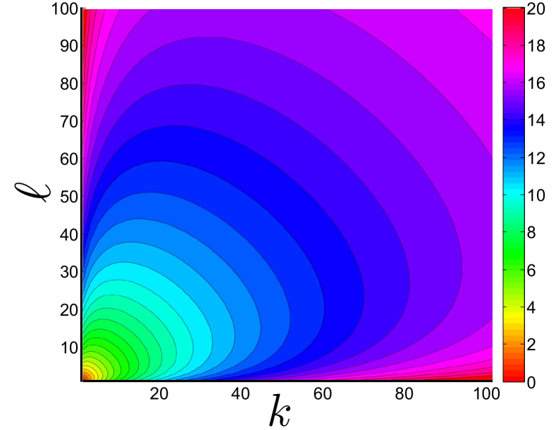
Figure 1: (Color online) The joint degree distribution for preferential growth with $\beta_{1}=3$ and $\beta_{2}=3$. Theoretical result is presented in (6). Since the values decay fast in $k$ and $\ell$, we have depicted the logarithm of the inverse of this function, for a smoother output and better visibility. The joint distribution attains its maximum at $k=\beta_{1}$ and $\ell=\beta_{2}$. The contours are symmetric with respect to the bisector because $\beta_{1}$ and $\beta_{2}$ are equal. Note that each axis begins at its corresponding value of $\beta$, so the origin is $\beta_{1},\beta_{2}$.

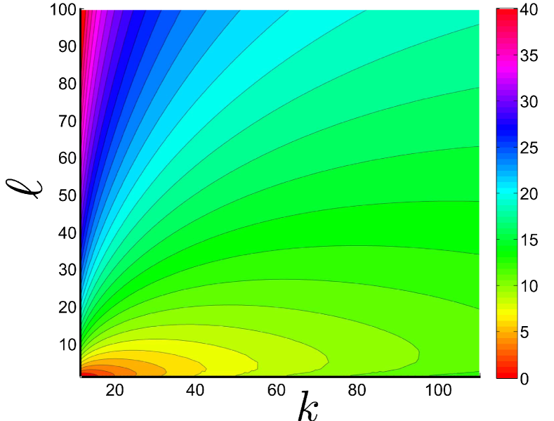
Figure 2: (Color online) logarithm of the inverse of the joint degree distribution for preferential growth with $\beta_{1}=10$ and $\beta_{2}=2$. Theoretical solution is presented in (6). The joint distribution attains its maximum at $k=\beta_{1}$ and $\ell=\beta_{2}$. The contours are skewed towards the $k$ axis because $\beta_{1}>\beta_{2}$. Note that each axis begins at its corresponding value of $\beta$, so the origin is $\beta_{1},\beta_{2}$.

Let us verify (6) via simulations. For the first setup, we consider $\beta_{1}=4$ and $\beta_{2}=3$, and plot $n(k,\ell)$ for multiple example instances of $k$ and $\ell$. The initial seed networks are identical star graphs with 6 nodes in both layers. The results are depicted in Figure 3. We observe that the simulation results reach the horizontal asymptotes predicted by (6) relatively early on in the process. When the size of the network is $N=300$, the effects of the initial seed graph are already negligible. For the second example, we consider $\beta_{1}=2$ and $\beta_{2}=3$. For the initial seed network, we consider complete graphs with 4 nodes in both layers. The results are depicted in Figure 4. We again observe convergence to the theoretical predictions. Moreover, we observe that equilibrium emerges when the size of the network is 20 times the size of the initial seed network. Note that the asymptotes in Figure 3 and those of Figure 4 differ, because they pertain to different growth parameters.

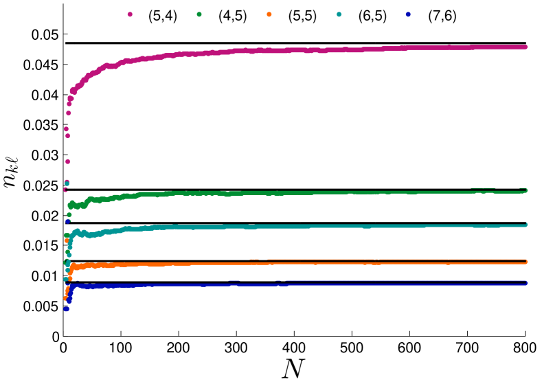
Figure 3: (Color online) Comparison between the steady-state joint degree distribution and the theoretical prediction of (6) for growth under preferential attachment with growth parameters $\beta_{1}=4$ and $\beta_{2}=3$. The horizontal lines represent the steady-state asymptotes which accord with (6), and markers represent simulation results. The initial seed networks are star graphs with 6 nodes in both layers. Several example value of $(k,\ell)$ are chosen for illustrative purposes. The results are averaged over 100 Monte Carlo trials.

Figure 4: (Color online) Comparison between the steady-state joint degree distribution and the theoretical prediction of (6) for growth under preferential attachment with growth parameters $\beta_{1}=2$ and $\beta_{2}=3$. The horizontal lines represent the steady-state asymptotes which accord with (6), and markers represent simulation results. The initial seed networks are complete graphs with 4 nodes in both layers. Several example value of $(k,\ell)$ are chosen for illustrative purposes. The results are averaged over 100 Monte Carlo trials.

We can see the entanglement between the two layers through the conditional average degree, which can be derived from (6). For the nodes who have degree $k$ in layer 1, we can find their average degree in layer 2. Let us denote this quantity by $\bar{\ell}(k)$. In the calculations, the marginal degree distribution of layer 1 is invoked. This is obtained in Dorogovtsev et al. (2000); Krapivsky et al. (2000), and we also obtain it in Equation (35) in Section IV—as a byproduct of our calculations. We use this expression in the calculation of the conditional degree. To find the conditional degree, we need to perform the following summation:

$$\bar{\ell}(k) =\,\displaystyle\sum_{\ell}\ell n(\ell|k)=\,\displaystyle\sum_{\ell}\ell\,\displaystyle\frac{n(k,\ell)}{n_{k}}$$

$$=\,\displaystyle\sum_{\ell}\ell\,\displaystyle\frac{\frac{2\beta_{1}(\beta_{1}+1)\beta_{2}(\beta_{2}+1)}{(2+\beta_{1}+\beta_{2})k(k+1)\ell(\ell+1)}\frac{\,\binom{\beta_{1}+\beta_{2}+2}{\beta_{1}+1}}{\,\binom{k+\ell+2}{k+1}}\,\binom{k-\beta_{1}+\ell-\beta_{2}}{k-\beta_{1}}}{\frac{2\beta_{1}(\beta_{1}+1)}{k(k+1)(k+2)}}$$

$$=\,\displaystyle\sum_{\ell}\frac{\beta_{2}(\beta_{2}+1)(k+2)}{(2+\beta_{1}+\beta_{2})(\ell+1)}\frac{\,\binom{\beta_{1}+\beta_{2}+2}{\beta_{1}+1}\,\binom{k-\beta_{1}+\ell-\beta_{2}}{k-\beta_{1}}}{\,\binom{k+\ell+2}{k+1}}$$

$$=\,\displaystyle\sum_{\ell}\frac{\beta_{2}(\beta_{2}+1)}{(2+\beta_{1}+\beta_{2})}\frac{\,\binom{\beta_{1}+\beta_{2}+2}{\beta_{1}+1}\,\binom{k-\beta_{1}+\ell-\beta_{2}}{k-\beta_{1}}}{\,\binom{k+\ell+2}{\ell}}$$ (8)

In Appendix B, we perform this summation. The answer is

$$\bar{\ell}(k)=\,\displaystyle\frac{\beta_{2}}{\beta_{1}+1}(k+2).$$ (9)

In the special case of $\beta_{1}=\beta_{2}=m$, this reduces to $\frac{m(k+2)}{1+m}$, which is consistent with the previous result in the literature Nicosia et al. (2013).

We now focus on the distribution of total degree (i.e., the sum of degrees in the two layers). Let us denote $k+\ell$ by $q$. The joint distribution of $q,k$ is simply ${n(k,q-k)}$. If we sum over all possible values of $k$, we get the distribution of $q$. Note that $k$ is at least $\beta_{1}$, because every incoming node has an initial degree of $\beta_{1}$ in the first layer upon birth. Similarly, note that $q-k_{1}$ is at least $\beta_{2}$. Taking these two into account for the summation bounds, we have:

$$n(q)= \,\displaystyle\frac{2\beta_{1}(\beta_{1}+1)\beta_{2}(\beta_{2}+1)\,\binom{\beta_{1}+\beta_{2}+2}{\beta_{1}+1}}{(2+\beta_{1}+\beta_{2})}$$

$$\times\,\displaystyle\sum_{k=\beta_{1}}^{q-\beta_{2}}\,\displaystyle\frac{\,\binom{q-\beta_{1}-\beta_{2}}{k-\beta_{1}}}{k(k+1)(q-k)(q-k+1)\,\binom{q+2}{k+1}}$$

$$= \,\displaystyle\frac{2\beta_{1}(\beta_{1}+1)\beta_{2}(\beta_{2}+1)\,\binom{\beta_{1}+\beta_{2}+2}{\beta_{1}+1}}{(2+\beta_{1}+\beta_{2})(q+2)(q+1)q(q-1)}\,\displaystyle\sum_{k=\beta_{1}}^{q-\beta_{2}}\,\displaystyle\frac{\,\binom{q-\beta_{1}-\beta_{2}}{k-\beta_{1}}}{\,\binom{q-2}{k-1}}.$$

We use the following identity:

$$\,\displaystyle\sum_{k=\beta_{1}}^{q-\beta_{2}}\,\displaystyle\frac{\,\binom{q-\beta_{1}-\beta_{2}}{k-\beta_{1}}}{\,\binom{q-2}{k-1}}=\,\displaystyle\frac{(\beta_{1}-1)!(\beta_{2}-1)!(q-1)}{(\beta_{2}+\beta_{1}-1)!}.$$ (11)

This is proven in Appendix C. Plugging this result into (10), we arrive at

$$n(q)=\,\displaystyle\frac{2(\beta_{1}+\beta_{2})(\beta_{1}+\beta_{2}+1)}{q(q+1)(q+2)}u(q-\beta_{1}-\beta_{2}),$$ (12)

where $u(\cdot)$ is the Heaviside step function. This is identical to the expression for a single-layer network growing under growth parameter ${\beta_{1}+\beta_{2}}$. In other words, the aggregated network is tantamount to one which grows under the preferential attachment mechanism where each incoming node establishes $\beta_{1}+\beta_{2}$ links to existing nodes, which is intuitively expected.

III Model 2: Uniform Attachment in Two Layers

In this model, we assume that each incoming node establishes its link in both layers by selecting existing nodes uniformly at random. The rate equation (2) in the case of uniform attachment transforms into

$$N_{t+1}(k,\ell)=N_{t}({k,\ell})+\beta_{1}\,\displaystyle\frac{N_{t}(k-1,\ell)-N_{t}(k,\ell)}{N(0)+t}$$

$$+\beta_{2}\,\displaystyle\frac{N_{t}(k,\ell-1)-N_{t}(k,\ell)}{N(0)+t}+\delta_{k\beta_{1}}\delta_{\ell\beta_{2}}.$$ (13)

Using the substitution $n_{k,\ell}(t)=\frac{N_{t}(k,\ell)}{N(0)+t}$, this becomes

$$\big{[}N(0)+t\big{]}\big{[}n_{t+1}(k,\ell)-n_{t}(k,\ell)\big{]}+n_{t+1}(k,\ell)=$$

$$+\beta_{1}\,\displaystyle\frac{N_{t}(k-1,\ell)-N_{t}(k,\ell)}{N(0)+t}$$

$$+\beta_{2}\,\displaystyle\frac{N_{t}(k,\ell-1)-N_{t}(k,\ell)}{N(0)+t}+\delta_{k\beta_{1}}\delta_{\ell\beta_{2}},$$ (14)

which simplifies to the following difference equation in the limit as ${t\rightarrow\infty}$, that is, the steady state:

$$n(k,\ell)= \beta_{1}\,\displaystyle\frac{n(k-1,\ell)-n(k,\ell)}{1}+\beta_{2}\,\displaystyle\frac{n(k,\ell-1)-n(k,\ell)}{1}$$

$$+\delta_{k,\beta_{1}}\delta_{\ell,\beta_{2}}.$$ (15)

This can be simplified and equivalently expressed as follows

(16)

This difference equation is solved in Appendix D. The solution is

$$n(k,\ell)=\,\displaystyle\frac{\beta_{1}^{k-\beta_{1}}\beta_{2}^{\ell-\beta_{2}}\,\binom{k-\beta_{1}+\ell-\beta_{2}}{k-\beta_{1}}}{(1+\beta_{1}+\beta_{2})^{k-\beta_{1}+\ell-\beta_{2}+1}}.$$ (17)

This result agrees with the findings in Fotouhi and Momeni (2015), and those in Nicosia et al. (2013, 2014)—in the special case of $\beta_{1}=\beta_{2}$.

Figure 5 represents the joint degree distribution for the case of $\beta_{1}=\beta_{2}=3$. We plotted the logarithm of the inverse of this function for smoothness and visibility purposes. Figure 6 depicts the joint distribution for the case of $\beta_{1}=10$ and $\beta_{2}=2$. Note that in both cases, since the joint degree distribution is nonzero only for $k>\beta_{1}$ and $\ell>\beta_{2}$, the origin is situated at $\beta_{1},\beta_{2}$.

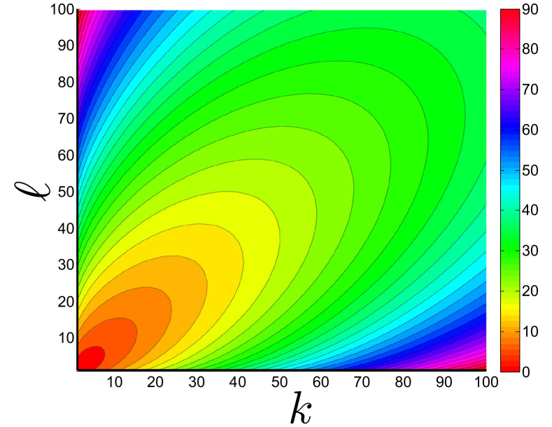
Figure 5: (Color online) The joint degree distribution for uniform growth with $\beta_{1}=3$ and $\beta_{2}=3$. Theoretical result is presented in (17). Since the values decay fast in $k$ and $\ell$, we have depicted the logarithm of the inverse of this function, for a smoother output and better visibility. The joint distribution attains its maximum at $k=\beta_{1}$ and $\ell=\beta_{2}$. The contours are symmetric with respect to the bisector because $\beta_{1}$ and $\beta_{2}$ are equal. Note that each axis begins at its corresponding value of $\beta$, so the origin is $\beta_{1},\beta_{2}$.

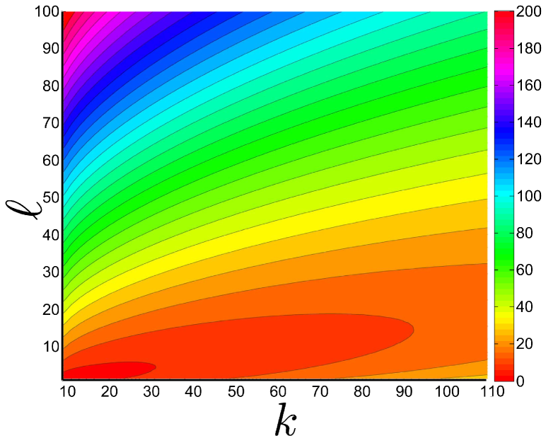
Figure 6: (Color online) logarithm of the inverse of the joint degree distribution for uniform growth with $\beta_{1}=10$ and $\beta_{2}=2$. Theoretical solution is presented in (6). The joint distribution attains its maximum at $k=\beta_{1}$ and $\ell=\beta_{2}$. The contours are skewed towards the $k$ axis because $\beta_{1}>\beta_{2}$. Note that each axis begins at its corresponding value of $\beta$, so the origin is $\beta_{1},\beta_{2}$.

Let us verify (17) via simulations. For the first setup, we consider $\beta_{1}=5$ and $\beta_{2}=8$. We plot $n(k,\ell)$ for multiple example instances of $k$ ad $\ell$.The initial seed networks in both layers are rings with 10 nodes. The results are illustrated in Figure 7. The simulation results visibly converge to the theoretical predictions. Moreover, equilibrium emerges relatively early, that is, even when the size of the network is 200, which is only 20 times the size of the initial seed network, the effects of the initial nodes are already negligible. For the second example, we consider the symmetric case $\beta_{1}=\beta_{2}=10$. For the initial seed network, we consider complete graphs with $15$ nodes in both layers. The results are depicted in Figure 8. The results again verify the steady-state prediction, and confirm that equilibrium emerges relatively early on in the process, namely, when the size of the network is 20 times the size of the seed network.

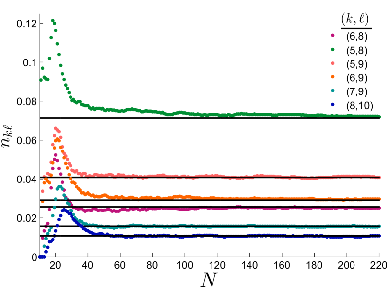
Figure 7: (Color online) Comparison between the steady-state joint degree distribution and the theoretical prediction of (17) for growth under uniform attachment with growth parameters $\beta_{1}=5$ and $\beta_{2}=8$. The horizontal lines represent the steady-state solution given by (17), and markers represent simulation results. The initial seed networks are rings with 10 nodes in both layers. The simulation results are averaged over 100 Monte Carlo trials.

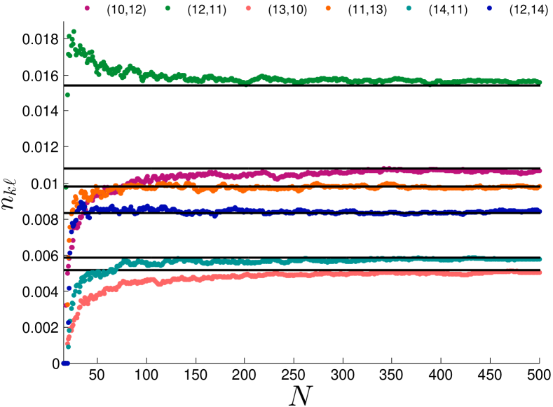
Figure 8: (Color online) Comparison between the steady-state joint degree distribution and the theoretical prediction of (17) for growth under uniform attachment with growth parameters $\beta_{1}=\beta_{2}=10$. The horizontal lines represent the steady-state asymptotes which accord with (17), and markers represent simulation results. The initial seed networks are complete graphs with 15 nodes in both layers. Several example value of $(k,\ell)$ are chosen for illustrative purposes. The results are averaged over 100 Monte Carlo trials.

To find the conditional average degree, we first need the degree distribution of single layers. This is found previously for example in Fotouhi and Rabbat (2013); Nicosia et al. (2013). The degree distribution in the first layer is

$$n_{k}=\frac{1}{\beta_{1}}\left(\,\displaystyle\frac{\beta_{1}}{\beta_{1}+1}\right)^{k-\beta_{1}+1}$$ (18)

We need to compute

$$\bar{\ell}(k) =\,\displaystyle\sum_{\ell}\ell n(\ell|k)=\,\displaystyle\sum_{\ell}\ell\,\displaystyle\frac{n(k,\ell)}{n_{k}}$$

$$=\,\displaystyle\sum_{\ell}\ell\,\displaystyle\frac{\,\displaystyle\frac{\beta_{1}^{k-\beta_{1}}\beta_{2}^{\ell-\beta_{2}}\,\binom{k-\beta_{1}+\ell-\beta_{2}}{k-\beta_{1}}}{(1+\beta_{1}+\beta_{2})^{k-\beta_{1}+\ell-\beta_{2}+1}}}{\frac{1}{\beta_{1}}\left(\frac{\beta_{1}}{\beta_{1}+1}\right)^{k-\beta_{1}+1}}$$

$$=\,\displaystyle\frac{(\beta_{1}+1)^{k-\beta_{1}+1}}{(\beta_{1}+\beta_{2}+1)^{k-\beta_{1}+1}}\,\displaystyle\sum_{\ell}\ell\frac{\beta_{2}^{\ell-\beta_{2}}\,\binom{k-\beta_{1}+\ell-\beta_{2}}{k-\beta_{1}}}{(1+\beta_{1}+\beta_{2})^{\ell-\beta_{2}}}$$ (19)

We have performed this summation in Appendix E. The result is

$$\bar{\ell}(k)=\frac{\beta_{2}}{\beta_{1}+1}(k+2).$$ (20)

This is identical to (9). For the special case of $\beta_{1}=\beta_{2}$, this result (that the expected degree has the same expression under preferential and uniform attachment schemes) is also obtained in Nicosia et al. (2013)—see Equations (S.40) and (S.45) therein.

Finally, to obtain the distribution of total degree, we undertake the steps similar to those in the previous section. We have:

$$n(q) =\,\displaystyle\sum_{k}n(k,q-k)$$

$$=\,\displaystyle\sum_{k}\,\displaystyle\frac{\beta_{1}^{k-\beta_{1}}\beta_{2}^{q-k-\beta_{2}}\,\binom{q-\beta_{1}-\beta_{2}}{k-\beta_{1}}}{(1+\beta_{1}+\beta_{2})^{q-\beta_{1}-\beta_{2}+1}}$$

$$=\,\displaystyle\frac{\beta_{2}^{q-\beta_{2}-\beta_{1}}}{(1+\beta_{1}+\beta_{2})^{q-\beta_{1}-\beta_{2}+1}}\,\displaystyle\left(1+\frac{\beta_{1}}{\beta_{2}}\right)^{q-\beta_{1}-\beta_{2}}$$

$$=\,\displaystyle\frac{1}{\beta_{1}+\beta_{2}}\,\displaystyle\left(\,\displaystyle\frac{\beta_{1}+\beta_{2}}{1+\beta_{1}+\beta_{2}}\right)^{q-\beta_{1}-\beta_{2}}.$$ (21)

This is similar to (18). This means that the degree distribution of the aggregated network is identical to that of a uniformly growing network in which each newcomer forms $\beta_{1}+\beta_{2}$ links to existing nodes.

IV Generalization of Model 1 to $M$ Layers

Now let us consider the case of $M$ layers, where the network possesses one set of nodes and $M$ distinct sets of links. Each incoming node establishes $\beta_{m}$ links in layer $m$ to existing nodes in that layer, where ${m\in\{1,2,\ldots,M\}}$. The initial number of links at layer $m$ is denoted by $L_{m}(0)$. In this model, the degree of each node can be conveniently represented by a vector of length $M$. The degree vector of node $x$, denoted by $\mathbf{k}_{x}$, stores the degree of node $x$ in layer $m$ as its $m$-th component. Let $N(\mathbf{k})$ denote the number of nodes whose vector of degrees is $\mathbf{k}$. Let $n(\mathbf{k})$ denote the fraction of those nodes. If node $x$ receives a link in layer $m$, then its degree will change to ${\mathbf{k}+1\mathbf{e}_{m}}$, where $\mathbf{e}_{m}$ is the unit vector in $m$-th dimension, that is, it is a vector whose elements are all zero except its $m$-th element, which is unity. Let us denote the $m$th component of vector $\mathbf{k}$ by $k_{m}$. The rate equation for $N(\mathbf{k})$ reads

$$N_{t+1}(\mathbf{k})= N_{t}(\mathbf{k})+\,\displaystyle\prod_{m=1}^{M}\delta_{k_{m},\beta_{m}}$$

$$+\,\displaystyle\sum_{m=1}^{M}\beta_{m}\,\displaystyle\frac{(k_{m}-1)N_{t}(\mathbf{k}-\mathbf{e}_{m})-(k_{m})N_{t}(\mathbf{k})}{L_{m}(0)+2\beta_{m}t}$$ (22)

Now we use $N_{t}(\mathbf{k})=\frac{n_{t}(\mathbf{k})}{N(0)+t}$, and the following limit:

$$\lim_{t\rightarrow\infty}\beta_{m}\,\displaystyle\frac{N(0)+t}{L_{m}(0)+2\beta_{m}t}=\frac{1}{2}.$$ (23)

With these substitutions, we can rewrite (22) in the steady state as follows

$$n(\mathbf{k})= \frac{1}{2}\,\displaystyle\sum_{m=1}^{M}\bigg{[}(k_{m}-1)n(\mathbf{k}-\mathbf{e}_{m})-(k_{m})n(\mathbf{k})\bigg{]}$$

$$+\,\displaystyle\prod_{m=1}^{M}\delta_{k_{m},\beta_{m}}$$ (24)

This can be rearranged and expressed equivalently as follows

$$n(\mathbf{k})= \,\displaystyle\sum_{m=1}^{M}\bigg{[}\,\displaystyle\frac{k_{m}-1}{2+\sum_{m=1}^{M}k_{m}}n(\mathbf{k}-\mathbf{e}_{m})\bigg{]}$$

$$+\,\displaystyle\frac{2}{2+\sum_{m=1}^{M}\beta_{m}}\,\displaystyle\prod_{m=1}^{M}\delta_{k_{m},\beta_{m}}$$ (25)

We first define the following auxiliary function:

$$\phi(\mathbf{k})\,\stackrel{{\scriptstyle\text{def}}}{{=}}\,\displaystyle\frac{(2+\sum_{m=1}^{M}k_{m})!}{\prod_{m=1}^{M}(k_{m}-1)!}n(\mathbf{k})$$ (26)

Inserting this into (25) yields the following simplified equation

$$\phi(\mathbf{k}) =\sum_{m=0}^{M}\phi(\mathbf{k}-\mathbf{e}_{m})+2\,\displaystyle\frac{(2+\sum_{m=1}^{M}k_{m})!}{\prod_{m=1}^{M}(k_{m}-1)!}\,\displaystyle\prod_{m=1}^{M}\delta_{k_{m},\beta_{m}}$$

$$=\sum_{m=0}^{M}\phi(\mathbf{k}-\mathbf{e}_{m})+2\,\displaystyle\frac{(2+\sum_{m=1}^{M}\beta_{m})!}{\prod_{m=1}^{M}(\beta_{m}-1)!}\,\displaystyle\prod_{m=1}^{M}\delta_{k_{m},\beta_{m}}$$ (27)

We define the $M$-dimensional Z-transform as follows:

$$\Phi(\mathbf{z})\,\stackrel{{\scriptstyle\text{def}}}{{=}}\sum_{k_{1}=0}^{\infty}\sum_{k_{2}=0}^{\infty}\ldots\sum_{k_{M}=0}^{\infty}\phi(\mathbf{z})z^{-k1-k2-\ldots-k_{M}}.$$ (28)

Plugging this into (27), we obtain

$$\Phi(\mathbf{z})=2\,\displaystyle\frac{(2+\sum_{m=1}^{M}\beta_{m})!}{\prod_{m=1}^{M}(\beta_{m}-1)!}\,\displaystyle\frac{\,\displaystyle\prod_{m=1}^{M}z_{m}^{-\beta_{m}}}{1-\sum_{m=0}^{M}z_{m}^{-1}}.$$ (29)

The inverse of this generating function is given by

$$\leavevmode\resizebox{433.62pt}{}{$\phi(\mathbf{k})=2\,\displaystyle\frac{(2+\sum_{m=1}^{M}\beta_{m})!}{\prod_{m=1}^{M}(\beta_{m}-1)!}\oint\,\displaystyle\prod_{m=1}^{M}\,\displaystyle\frac{z_{m}^{k_{m}-\beta_{m}-1}}{1-\sum_{m=0}^{M}z_{m}^{-1}}\frac{d\mathbf{z_{m}}}{(2\pi i)^{M}}$}.$$ (30)

$$\,\displaystyle\frac{1}{{(2\pi i)^{M}}}\,\displaystyle\oint\,\displaystyle\prod_{m=1}^{M}\,\displaystyle\frac{z_{m}^{k_{m}-\beta_{m}-1}}{1-\sum_{m=0}^{M}z_{m}^{-1}}dz_{m}=\,\displaystyle\frac{1}{{(2\pi i)^{M}}}\,\displaystyle\oint\,\displaystyle\prod_{m=1}^{M}z_{m}^{k_{m}-\beta_{m}-1}dz_{m}\sum_{n=0}^{\infty}\left[\sum_{m=0}^{M}z_{m}^{-1}\right]^{n}$$

$$=\,\displaystyle\frac{1}{{(2\pi i)^{M}}}\,\displaystyle\oint\,\displaystyle\prod_{m=1}^{M}z_{m}^{k_{m}-\beta_{m}-1}dz_{m}\sum_{n=0}^{\infty}\sum_{r_{1}+\ldots+r_{M}=n}\,\binom{n}{r_{1},\ldots,r_{M}}\prod_{s=1}^{M}z_{1}^{-r_{s}}$$

$$=\,\displaystyle\sum_{n=0}^{\infty}\sum_{r_{1}+\ldots+r_{M}=n}\,\binom{n}{r_{1},\ldots,r_{M}}\prod_{s=1}^{M}\delta\big{[}r_{s}-(k_{m}-\beta_{m})\big{]}=\,\binom{\sum_{m=1}^{M}(k_{m}-\beta_{m})}{k_{1}-\beta_{1},\ldots,k_{m}-\beta_{M}}.$$ (31)

Inserting this result into (30), we arrive at

$$\phi(\mathbf{k})=2\,\displaystyle\frac{(2+\sum_{m=1}^{M}\beta_{m})!}{\prod_{m=1}^{M}(\beta_{m}-1)!}\,\displaystyle\,\binom{\sum_{m=1}^{M}(k_{m}-\beta_{m})}{k_{1}-\beta_{1},\ldots,k_{m}-\beta_{M}}.$$ (32)

Finally, from (26) we obtain

$$n(\mathbf{k})= \,\displaystyle\frac{\prod_{m=1}^{M}(k_{m}-1)!}{\prod_{m=1}^{M}(\beta_{m}-1)!}\,\displaystyle\frac{(2+\sum_{m=1}^{M}\beta_{m})!}{(2+\sum_{m=1}^{M}k_{m})!}$$

$$\times\,\displaystyle\frac{2}{2+\sum_{m=1}^{M}\beta_{m}}\,\displaystyle\,\binom{\sum_{m=1}^{M}(k_{m}-\beta_{m})}{k_{1}-\beta_{1},\ldots,k_{m}-\beta_{M}}.$$ (33)

Note that this expression holds for ${k_{m}\geq\beta_{m}}$, for all $M$ layers. If any of the $k_{m}$ values are smaller than the corresponding $\beta_{m}$ value, then $n(\mathbf{k})$ is zero. This is true because every node has an initial degree of $\beta_{m}$ in layer $m$ upon birth, and throughout the growth process, the degrees cannot decrease.

Now let us consider some special cases in order to gain insight into the pattern (33) follows. For $M=1$, we have:

$$n(k)=\,\displaystyle\frac{(k-1)!}{(\beta-1)!}\,\displaystyle\frac{(2+\beta)!}{(2+k)!}\times\,\displaystyle\frac{2}{2+\beta}\,\binom{k-\beta}{k-\beta}.$$ (34)

It can be easily simplified and rewritten as follows:

$$n(k)=\,\displaystyle\frac{(k-1)!}{(\beta-1)!}\,\displaystyle\frac{(\beta+2)!}{(k+2)!}\,\displaystyle\frac{2}{\beta+2}=\,\displaystyle\frac{2\beta(\beta+1)}{k(k+1)(k+2)}.$$ (35)

This agrees with the degree distribution of the preferential attachment model for a single layer, obtained for example in Dorogovtsev et al. (2000); Krapivsky et al. (2000).

Now let us consider the special case of $M=2$ and verify that (33) indeed reduces to (7). For $M=2$ we have:

$$n(k_{1},k_{2}) =\,\displaystyle\frac{(k_{1}-1)!(k_{2}-1)!}{(\beta_{1}-1)!(\beta_{2}-1)!}\,\displaystyle\frac{(2+\beta_{1}+\beta 2)!}{(2+k_{1}+k_{2})!}$$

$$\times\,\displaystyle\frac{2}{2+\beta_{1}+\beta_{2}}\,\displaystyle\frac{(k_{1}-\beta_{1}+k_{2}-\beta_{2})!}{(k_{1}-\beta_{1})!(k_{2}-\beta_{2})!}.$$ (36)

Note that the factor ${(2+\beta_{1}+\beta_{2})!}$ that exists in the numerator of the second fraction on the right hand side simplifies into ${(1+\beta+1+\beta_{2})!}$, due to the existence of the factor ${2+\beta_{1}+\beta_{2}}$ in the denominator of the third fraction. Applying this change, the result becomes identical to the expression obtained in (7).

Finally, let us inspect the form of (33) for $M=3$. For three layers, we have:

$$n(k_{1},k_{2},k_{3})$$

$$=\,\displaystyle\frac{(k_{1}-1)!(k_{2}-1)!(k_{3}-1)!}{(\beta_{1}-1)!(\beta_{2}-1)!(\beta_{3}-1)!}\,\displaystyle\frac{(2+\beta_{1}+\beta 2+\beta_{3})!}{(2+k_{1}+k_{2}+k_{3})!}$$

$$\times\,\displaystyle\frac{2}{2+\beta_{1}+\beta_{2}+\beta_{3}}\,\displaystyle\frac{(k_{1}-\beta_{1}+k_{2}-\beta_{2}+k_{3}-\beta_{3})!}{(k_{1}-\beta_{1})!(k_{2}-\beta_{2})!(k_{3}-\beta_{3})!}.$$ (37)

The pattern for general $M$ is clear from these three cases.

Let us verify the theoretical prediction in (33) via simulations. We consider three layers, and an initial seed network with 5 nodes. In layer 1, the nodes are situated on a ring. In layer 2, the topology is a star. In layer 3, we have a complete graph. The growth parameters are $\beta_{1}=2$, $\beta_{2}=3$, and $\beta_{3}=4$. Figure 9 depicts the results for multiple example ${(k_{1},k_{2},k_{3})}$ triplets. In all cases, the simulation results visibly converge to the horizontal asymptotes predicted by (33).

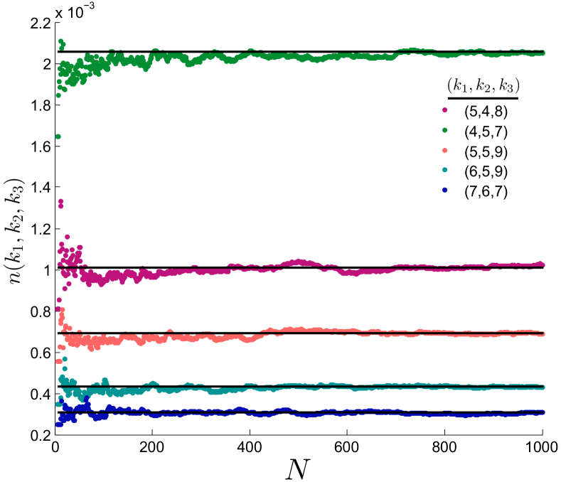
Figure 9: (Color online) Comparison between the steady-state three-layer joint degree distribution and the theoretical result of (33) for the case of preferential attachment. The horizontal lines represent the steady-state asymptotes predicted by (33), and markers represent simulation results, which are averaged over 100 Monte Carlo trials. The initial seed networks have 5 nodes, and the topologies in the three layers are ring, star, and complete, respectively. The growth parameters are $\beta_{1}=2$, $\beta_{2}=3$, and $\beta_{3}=4$. Several example values of $(k_{1},k_{2},k_{3})$ are chosen for illustrative purposes.

V Generalization of Model 2 to M Layers

Now we assume that there are $M$ layers, all of them growing under uniform attachment. The rate equation reads

$$N_{t+1}(\mathbf{k})= N_{t}(\mathbf{k})+\,\displaystyle\prod_{m=1}^{M}\delta_{k_{m},\beta_{m}}$$

$$+\,\displaystyle\sum_{m=1}^{M}\beta_{m}\,\displaystyle\frac{N_{t}(\mathbf{k}-\mathbf{e}_{m})-N_{t}(\mathbf{k})}{N(0)+t}$$ (38)

For $n_{t}(\mathbf{k})$, this transforms into the following recurrence relation in the steady state

$$n(\mathbf{k})=\,\displaystyle\prod_{m=1}^{M}\delta_{k_{m},\beta_{m}}+\,\displaystyle\sum_{m=1}^{M}\beta_{m}\bigg{[}n_{t}(\mathbf{k}-\mathbf{e}_{m})-n_{t}(\mathbf{k})\bigg{]}$$ (39)

This can be rearranged and recast as

$$n(\mathbf{k})=\,\displaystyle\frac{\,\displaystyle\prod_{m=1}^{M}\delta_{k_{m},\beta_{m}}}{1+\sum_{m=1}^{M}\beta_{m}}+\,\displaystyle\sum_{m=1}^{M}\beta_{m}\,\displaystyle\frac{\bigg{[}n_{t}(\mathbf{k}-\mathbf{e}_{m})\bigg{]}}{1+\sum_{m=1}^{M}\beta_{m}}$$ (40)

Let us define

$$\begin{cases}B\,\stackrel{{\scriptstyle\text{def}}}{{=}}1+\sum_{m=1}^{M}\beta_{m}\\ q_{m}\,\stackrel{{\scriptstyle\text{def}}}{{=}}\,\displaystyle\frac{\beta_{m}}{B}\end{cases}$$ (41)

Taking the generating function of two sides of (40), we get

$$\psi(\mathbf{z})=\,\displaystyle\frac{1}{B}\,\displaystyle\prod_{m=1}^{M}z_{m}^{-\beta_{m}}+\psi(\mathbf{z})\,\displaystyle\sum_{m=1}^{M}q_{m}z_{m}^{-1}.$$ (42)

This can be equivalently expressed as follows

$$\psi(\mathbf{z})=\,\displaystyle\frac{1}{B}\,\displaystyle\frac{\,\displaystyle\prod_{m=1}^{M}z_{m}^{-\beta_{m}}}{1-\,\displaystyle\sum_{m=1}^{M}q_{m}z_{m}^{-1}}.$$ (43)

The inverse of this generating function yields the desired degree distribution:

$$n(\mathbf{k})=\,\displaystyle\frac{1}{B}\,\displaystyle\frac{1}{(2\pi i)^{M}}\oint\,\displaystyle\frac{\,\displaystyle\prod_{m=1}^{M}z_{m}^{-\beta_{m}}z_{m}^{k_{m}-1}}{1-\,\displaystyle\sum_{m=1}^{M}q_{m}z_{m}^{-1}dz_{m}}.$$ (44)

We can perform the integration by undertaking the following successive steps:

$$\,\displaystyle\frac{1}{(2\pi i)^{M}}\oint\,\displaystyle\frac{\,\displaystyle\prod_{m=1}^{M}z_{m}^{-\beta_{m}}z_{m}^{k_{m}-1}dz_{m}}{1-\,\displaystyle\sum_{m=1}^{M}q_{m}z_{m}^{-1}}=\,\displaystyle\frac{1}{(2\pi i)^{M}}\oint\prod_{m=1}^{M}z_{m}^{k_{m}-\beta_{m}-1}dz_{m}\sum_{n=0}^{\infty}\bigg{[}\sum_{m=1}^{M}q_{m}z_{m}^{-1}\bigg{]}^{n}$$

$$=\,\displaystyle\frac{1}{(2\pi i)^{M}}\oint\prod_{m=1}^{M}z_{m}^{k_{m}-\beta_{m}-1}dz_{m}\sum_{n=0}^{\infty}\sum_{r_{1}+\ldots+r_{M}=n}\,\binom{n}{r_{1},\ldots,r_{M}}\prod_{s=1}^{M}q_{m}^{r_{s}}z_{m}^{-r_{s}}$$

$$=\sum_{n=0}^{\infty}\sum_{r_{1}+\ldots+r_{M}=n}\,\binom{n}{r_{1},\ldots,r_{M}}\prod_{s=1}^{M}q_{m}^{r_{s}}\delta_{r_{s},(k_{m}-\beta_{m})}$$

$$=\,\binom{\sum_{m=1}^{M}(k_{m}-\beta_{m})}{k_{1}-\beta_{1},\ldots,k_{M}-\beta_{M}}\prod_{m=1}^{M}q_{m}^{k_{m}-\beta_{m}}.$$ (45)

Plugging this result into (44), we get

$$n(\mathbf{k})=\frac{1}{B}\,\binom{\sum_{m=1}^{M}(k_{m}-\beta_{m})}{k_{1}-\beta_{1},\ldots,k_{M}-\beta_{M}}\prod_{m=1}^{M}q_{m}^{k_{m}-\beta_{m}}.$$ (46)

Using the definition of $B$ as given in (41), this can be expressed equivalently as follows:

$$n(\mathbf{k})=\frac{\,\binom{\sum_{m=1}^{M}(k_{m}-\beta_{m})}{k_{1}-\beta_{1},\ldots,k_{M}-\beta_{M}}\,\displaystyle\prod_{n=1}^{M}\beta_{n}^{k_{n}-\beta_{n}}}{\left(1+\sum_{m=1}^{M}\beta_{m}\right)^{1+\sum_{m=1}^{M}(k_{m}-\beta_{m})}}.$$ (47)

Note that, similar to the case of preferential growth, this expression holds for ${k_{m}\geq\beta_{m}}$, for all $M$ layers. If any of the $k_{m}$ values are smaller than the corresponding $\beta_{m}$ value, then $n(\mathbf{k})$ is zero.

Now we consider the special cases of $M=1,2,3$ and simplify this expression to gain more insight into the pattern it follows for general $M$, for convenience of interpretation.

For $M=1$, we have

$$n(k)=\frac{\,\binom{k-\beta}{k-\beta}\,\displaystyle\beta^{k-\beta}}{\left(1+\beta\right)^{1+(k-\beta)}}.$$ (48)

The binomial coefficient equals unity, and the result become identical to Equation (18), which is also obtained for example in Fotouhi and Rabbat (2013); Nicosia et al. (2013).

Now we focus on the special case of $M=2$, and confirm that it agrees with (17). Note that the multinomial coefficient in (47) becomes the ordinary binomial coefficient in this case. So for $M=2$ we have:

$$n(k_{1},k_{2})=\frac{\,\binom{k_{1}-\beta_{1}+k_{2}-\beta_{2}}{k_{1}-\beta_{1}}\,\displaystyle\beta_{1}^{k_{1}-\beta_{1}}\beta_{2}^{k_{2}\beta_{2}}}{\left(1+\beta_{1}+\beta_{2}\right)^{1+k_{1}-\beta_{1}+k_{2}-\beta_{2}}},$$ (49)

which is identical to Equation (18).

Finally, let us consider the case of $M=3$. We expand the multinomial coefficient into factorials to render the pattern for general $M$ more apparent. We have:

(50)

Let us verify the theoretical result of (47) via simulations. For the initial seed graph, consider 8 nodes which form complete graphs in layers one and three, and let them form a star graph in layer 2. Let the growth parameters be $\beta_{1}=3$, $\beta_{2}=4$, and $\beta_{3}=2$. Figure 10 depicts the results for multiple example ${(k_{1},k_{2},k_{3})}$ triplets. In all cases, it is visible that the simulation results converge to the horizontal asymptotes predicted by (47).

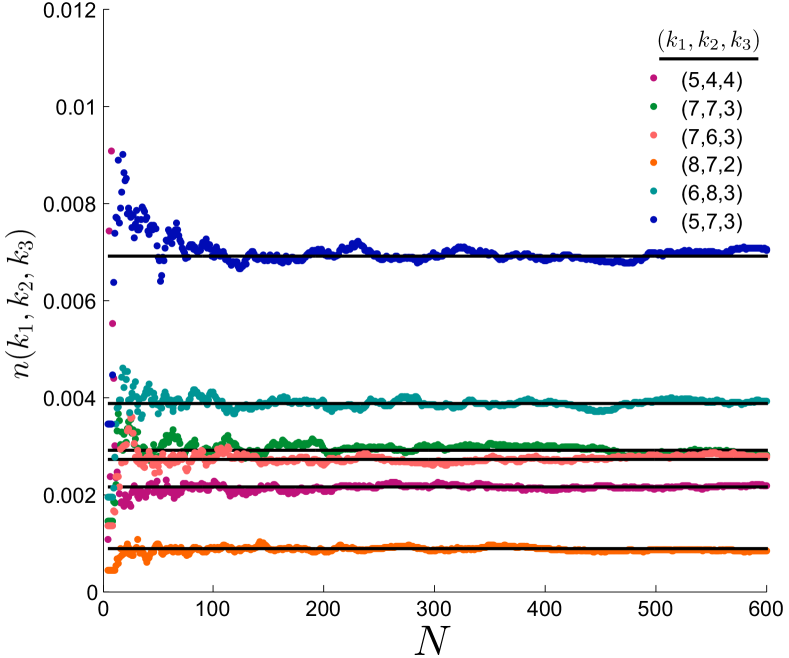
Figure 10: (Color online) Comparison between the steady-state three-layer joint degree distribution and the theoretical result of (47) for the case of uniform attachment. The horizontal lines represent the steady-state asymptotes predicted by (47), and markers represent simulation results, which are averaged over 100 Monte Carlo trials. The initial seed networks have 8 nodes, and the topologies in the three layers are complete, star, and complete, respectively. The growth parameters are $\beta_{1}=3$, $\beta_{2}=4$, and $\beta_{3}=2$. Several example values of $(k_{1},k_{2},k_{3})$ are chosen for illustrative purposes.

VI Temporal Evolution of the Joint Degree Distribution

We now move beyond the steady-state analysis and focus on the temporal evolution of the structure of multiplex networks. Consider a given multiplex network with $N(0)$ nodes, whose joint degree distribtuion is given by $n_{0}(\mathbf{k})$. How would $n(\mathbf{k})$ evolve if new nodes are added to the network? In this section, we seek a time-dependent solution for $n_{t}(\mathbf{k})$. We only consider the case where attachments are uniformly at random in each layer. Let us focus on the evolution of $N_{t}(\mathbf{k})$. At time $t$, upon the introduction of a single new node, we can rewrite the time-continuous analog of Equation (22) as follows:

$$\,\frac{\partial N_{t}(\mathbf{k})}{\partial t}= \,\displaystyle\prod_{m=1}^{M}\delta_{k_{m},\beta_{m}}$$

$$+\,\displaystyle\sum_{m=1}^{M}\beta_{m}\,\displaystyle\frac{N_{t}(\mathbf{k}-\mathbf{e}_{m})-N_{t}(\mathbf{k})}{N(0)+t}$$ (51)

Let us define the following generating function:

$$\Psi_{t}(z_{1},\ldots,z_{M})\stackrel{{\scriptstyle\text{def}}}{{=}}\sum_{k_{1}}\ldots\sum_{k_{M}}N_{t}(\mathbf{k})z_{1}^{-k_{1}}\ldots z_{M}^{-k_{M}}.$$ (52)

We now multiply both sides of (51) by ${z_{1}^{-k_{1}}\ldots z_{M}^{-k_{M}}}$, and sum over all $k_{i}$. The result is

$$\,\frac{\partial\Psi_{t}(z_{1},\ldots,z_{M})}{\partial t}=\prod_{i=1}^{M}z_{i}^{-\beta_{i}}$$

$$+\sum_{i=1}^{M}\,\displaystyle\frac{\beta_{i}}{N(0)+t}(z_{i}^{-1}-1)\Psi_{t}(z_{1},\ldots,z_{M}).$$ (53)

We can rearrange the terms and express this equation equivalently as follows:

(54)

This is a linear first order equation Boyce et al. (1992) which can be solved by the multiplication of both sides by the following integration factor:

$$\mu_{t}(z_{1},\ldots,z_{M})=\,\displaystyle\exp\int-\,\displaystyle\sum_{i=1}^{M}\,\displaystyle\frac{\beta_{i}(z_{i}^{-1}-1)}{N(0)+t}dt$$

$$=\exp\Bigg{[}-\ln(N(0)+t)\sum_{i=1}^{M}\beta_{i}(z_{i}^{-1}-1)\Bigg{]}$$

$$=(N(0)+t)^{-\sum_{i=1}^{M}\beta_{i}(z_{i}^{-1}-1)}$$ (55)

Using the integration factor, the solution is given by

$$\Psi_{t}(z_{1},\ldots,z_{M})=\mu^{-1}\,\displaystyle\Bigg{[}\int^{t}\prod_{i=1}^{M}z_{i}^{-\beta_{i}}\mu dt+C\Bigg{]}$$

$$=\mu^{-1}\left[\prod_{i=1}^{M}z_{i}^{-\beta_{i}}\,\displaystyle\frac{(N(0)+t)^{1-\sum_{i=1}^{M}\beta_{i}(z_{i}^{-1}-1)}}{1-\sum_{i=1}^{M}\beta_{i}(z_{i}^{-1}-1)}+C\right]$$

$$=(N(0)+t)\,\displaystyle\frac{\prod_{i=1}^{M}z_{i}^{-\beta_{i}}}{1-\sum_{i=1}^{M}\beta_{i}(z_{i}^{-1}-1)}$$

$$+C\,\displaystyle(N(0)+t)^{\sum_{i=1}^{M}\beta_{i}(z_{i}^{-1}-1)}.$$ (56)

In this equation, $C$ is a constant in time, but can depend on ${z_{1},\ldots,z_{M}}$. It must be determined in order to satisfy the initial conditions. Note that the generating function of the joint degree distribution of the initial network is known. So we can use $\Psi_{0}(z_{1},\ldots,z_{M})$ in order to identify $C$. Setting $t=0$ in (56), and rearranging the terms, we arrive at

$$C= \Psi_{0}(z_{1},\ldots,z_{M})\times N(0)^{-\sum_{i=1}^{M}\beta_{i}(z_{i}^{-1}-1)}$$

$$-\,\displaystyle\frac{\prod_{i=1}^{M}z_{i}^{-\beta_{i}}}{1-\sum_{i=1}^{M}\beta_{i}(z_{i}^{-1}-1)}N(0)^{1-\sum_{i=1}^{M}\beta_{i}(z_{i}^{-1}-1)}.$$ (57)

Finally, plugging this into (56) and rearranging the terms, we obtain the generating function of the joint degree distribution at arbitrary times:

$$+\Psi_{0}(z_{1},\ldots,z_{M})\times\left(1+\,\displaystyle\frac{t}{N(0)}\right)^{\sum_{i=1}^{M}\beta_{i}(z_{i}^{-1}-1)}$$

$$-\leavevmode\resizebox{368.57964pt}{}{$N(0)\left(1+\,\displaystyle\frac{t}{N(0)}\right)^{\sum_{i=1}^{M}\beta_{i}(z_{i}^{-1}-1)}\,\displaystyle\frac{\prod_{i=1}^{M}z_{i}^{-\beta_{i}}}{1-\sum_{i=1}^{M}\beta_{i}(z_{i}^{-1}-1)}$}.$$ (58)

Now we need to take the inverse of this transform. First let us take the inverse transform of ${G_{1}\stackrel{{\scriptstyle\text{def}}}{{=}}\frac{1}{1-\sum_{i=1}^{M}\beta_{i}(z_{i}^{-1}-1)}}$. We again denote $1+\sum_{m=1}^{M}\beta_{m}$ by $B$, and we denote $\frac{\beta_{m}}{B}$ by $q_{m}$, for brevity of notation. Using straightforward properties of geometric series and multinational expansions, we have:

$$G_{1}=\frac{1}{B}\,\displaystyle\frac{1}{1-\sum_{i}q_{i}z_{i}^{-1}}=\frac{1}{B}\sum_{m=1}^{\infty}(\sum_{i}q_{i}z_{i}^{-1})^{m}$$

$$=\frac{1}{B}\sum_{m}\sum_{r_{1}+\ldots+r_{M}=m}\,\binom{m}{r_{1},\ldots,r_{M}}\prod_{s=1}^{M}q_{s}^{r_{s}}z_{s}^{-r_{s}}.$$ (59)

The inverse transform of the expressions $z_{s}^{-r_{s}}$ is given by the delta function $\,\displaystyle\delta_{\,\displaystyle k_{s},r_{s}}$. Using this result, we get

$$G_{1}\xrightarrow{\mathcal{Z}^{-1}}\frac{1}{B}\sum_{m}\sum_{r_{1}+\ldots+r_{M}=m}\,\binom{m}{r_{1},\ldots,r_{M}}\prod_{s=1}^{M}\delta_{k_{s},r_{s}}q_{s}^{k_{s}}.$$ (60)

Applying the delta functions, all the sums reduce to a single nonvanishing term:

$$G_{1}\xrightarrow{\mathcal{Z}^{-1}}\frac{1}{B}\,\binom{\sum_{m=1}^{M}k_{m}}{k_{1},\ldots,k_{M}}\prod_{r=1}^{M}\,\displaystyle\frac{\beta_{r}^{k_{r}}}{B^{k_{r}}}.$$ (61)

The multiplication by $\prod_{i=1}^{M}z_{i}^{-\beta_{i}}$ merely results in shifts, that is, every $k_{r}$ changes to ${k_{r}-\beta_{r}}$. So we obtain

(62)

Now let us take the inverse transform of ${G_{2}\stackrel{{\scriptstyle\text{def}}}{{=}}\left(1+\frac{t}{N(0)}\right)^{\sum_{i=1}^{M}\beta_{i}z_{i}^{-1}}}$. Using elementary properties of the exponential function, we have

$$G_{2}=\prod_{m=1}^{M}\left(1+\frac{t}{N(0)}\right)^{\beta_{m}z_{m}^{-1}}$$

$$=\prod_{m=1}^{M}\exp\Bigg{[}\beta_{m}z_{m}^{-1}\ln\left(1+\frac{t}{N(0)}\right)\Bigg{]}$$

$$=\prod_{m=1}^{M}\sum_{r=1}^{\infty}\,\displaystyle\frac{\beta_{m}^{r}\left[\ln\left(1+\frac{t}{N(0)}\right)\right]^{r}}{r!}z_{m}^{-r}.$$ (63)

The inverse transform of the $z_{m}^{-r}$ terms yield delta functions, which helps us eliminate the sums. The result is

$$G_{2}\xrightarrow{\mathcal{Z}^{-1}}\prod_{m=1}^{M}\beta_{m}^{k_{m}}\,\displaystyle\frac{\left[\ln\left(1+\frac{t}{N(0)}\right)\right]^{k_{m}}}{k_{m}!}.$$ (64)

Plugging the expressions for the inverse transforms found in (62) and (64) into (58), and noting that the multiplication in the $z$ domain is equivalent to convolution in the $k$ domain, we arrive at the following expression for the inverse transform of ${\Psi_{t}(z_{1},\ldots,z_{M})}$, which is equal to $N_{t}(z_{1},\ldots,z_{M})$ by definition. Dividing the result by the number of nodes at time $t$, which is ${N(0)+t}$, we obtain the joint degree distribution as:

$$n_{t}(k_{1},\ldots,k_{M})=\,\displaystyle\frac{1}{B}\,\binom{\sum_{m=1}^{M}k_{m}-\beta_{m}}{k_{1}-\beta_{1},\ldots,k_{M}-\beta_{M}}\prod_{r=1}^{M}\,\displaystyle\frac{\beta_{r}^{k_{r}-\beta_{r}}}{B^{k_{r}-\beta_{r}}}$$

$$+\left(1+\,\displaystyle\frac{t}{N(0)}\right)^{-B}\,\displaystyle\sum_{\xi_{1},\ldots,\xi_{M}}n_{0}(\xi_{1},\ldots,\xi_{M})\prod_{m=1}^{M}\beta_{m}^{k_{m}-\xi_{m}}\,\displaystyle\frac{\left[\ln\left(1+\frac{t}{N(0)}\right)\right]^{k_{m}-\xi_{m}}}{(k_{m}-\xi_{m})!}$$

$$-\,\displaystyle\frac{1}{B}\left(1+\,\displaystyle\frac{t}{N(0)}\right)^{-B}\prod_{m=1}^{M}\beta_{r}^{k_{r}-\beta_{r}}B^{\beta_{m}}\,\displaystyle\sum_{\xi_{1}=\beta_{1}}^{k_{1}}\ldots\sum_{\xi_{M}=\beta_{M}}^{k_{M}}\,\binom{\sum_{m=1}^{M}\xi_{m}-\beta_{m}}{\xi_{1}-\beta_{1},\ldots,\xi_{M}-\beta_{M}}\prod_{m=1}^{M}\,\displaystyle\frac{\left[\ln\left(1+\frac{t}{N(0)}\right)\right]^{k_{m}-\xi_{m}}}{B^{\xi_{m}}(k_{m}-\xi_{m})!}.$$ (65)

The first term on the right hand side of (65) is independent of time, and is the steady-state solution which was obtained in (47). The second term characterizes the effect of the initial network. Note that the factor $\left(1+\frac{t}{N(0)}\right)^{-B-1}$ makes this term vanish in the long-time limit. This is expected, because in the limit as $t\rightarrow\infty$, almost every node is among those who were subsequently appended to the network, not those who belonged to the initial network. The last term on the right hand side is also transient and vanishes as time goes to infinity. At $t=0$, note that the first and third terms on the right hand side of (65) cancel out, and only the second term remains. In the second term, all the individual terms in the sum are zero (because the logarithm in the summand become $\log[1+0]$, which is zero), except one term, which pertains to ${\xi_{m}=k_{m}\forall m}$ (and for the logarithm, $0^{0}=1$), which means that the result correctly reduces to $n_{0}(k_{1},\ldots,k_{M})$.

For the special case of $M=2$, we get the following expression for the joint degree distribution of two layers:

$$n_{t}(k_{1},k_{2})=\,\binom{k_{1}-\beta_{1}+k_{2}-\beta_{2}}{k_{1}-\beta_{1}}\,\displaystyle\frac{\beta_{1}^{k_{1}-\beta_{1}}\beta_{2}^{k_{2}-\beta_{2}}}{(\beta_{1}+\beta_{2}+1)^{1+k_{1}-\beta_{1}+k_{2}-\beta_{2}}}$$

$$+\left(1+\,\displaystyle\frac{t}{N(0)}\right)^{-(\beta_{1}+\beta_{2}+1)}\sum_{\xi_{1},\xi_{2}}n_{0}(\xi_{1},\xi_{2})\beta_{1}^{k_{1}-\xi_{1}}\beta_{2}^{k_{2}-\xi_{2}}\,\displaystyle\frac{\left[\ln\left(1+\frac{t}{N(0)}\right)\right]^{k_{1}-\xi_{1}+k_{2}-\xi_{2}}}{(k_{1}-\xi_{1})!(k_{2}-\xi_{2})!}$$

$$\leavevmode\resizebox{411.93767pt}{}{$-\left(1+\,\displaystyle\frac{t}{N(0)}\right)^{-(\beta_{1}+\beta_{2}+1)}\,\displaystyle\frac{\beta_{1}^{k_{1}-\beta_{1}}\beta_{2}^{k_{2}-\beta_{2}}}{(\beta_{1}+\beta_{2}+1)^{1-\beta_{1}-\beta_{2}}}\,\displaystyle\sum_{\xi_{1}=\beta_{1}}^{k_{1}}\,\displaystyle\sum_{\xi_{2}=\beta_{2}}^{k_{2}}\,\displaystyle\frac{\,\displaystyle\,\binom{\xi_{1}-\beta_{1}+\xi_{2}-\beta_{2}}{\xi_{1}-\beta_{1}}\left[\ln\left(1+\frac{t}{N(0)}\right)\right]^{k_{1}-\xi_{1}+k_{2}-\xi_{2}}}{(\beta_{1}+\beta_{2}+1)^{\xi_{1}+\xi_{2}}(k_{1}-\xi_{1})!(k_{2}-\xi_{2})!}$}.$$ (66)

In the limit as $t\rightarrow\infty$, the second and third terms on the right hand side vanish, and the first term prevails, which coincides with the result obtained in (17).

Now let us verify the theoretical prediction for the time-dependent joint distribution via simulations. The first setup we consider is as follows. Consider 50 nodes with identical connectivity in both layers at time $t=0$, forming a ring. For the growth mechanism, consider $\beta_{1}=3$ and $\beta_{2}=2$. Figure 11 depicts $n_{t}(k_{1},k_{2})$ for some example test values for $k_{1}$ and $k_{2}$. It can be observed that simulation results are in good agreement with theoretical predictions.

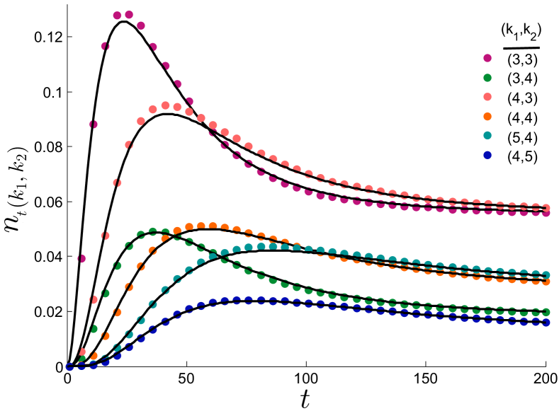
Figure 11: (Color online) Temporal evolution of the joint degree distribution for two layers. The growth parameters are $\beta_{1}=3$ and $\beta_{2}=2$. The solid curves represent theoretical prediction given by (66). The markers represent simulation results, averaged over 100 Monte Carlo trials.

For the second example, we consider the initial networks to be small-world graphs Newman and Watts (1999). We construct the initial networks in the following way. Consider a network of $N(0)$ nodes. Suppose that the nodes are situated on a circle and then each node is connected to $b$ immediate neighbors to the left and $b$ to the right. Then, each nonexistent link is established independently with probability $p$. We denote such a network by $SW(N(0),b,p)$, where $SW$ denotes small-world. For the second simulation setup, we consider a ${SW(200,0.05,2)}$ for the first layer and a ${SW(200,0.01,2)}$ for the second layer. We set the growth parameters to be $\beta_{1}=3$ and $\beta_{2}=4$. The results for several test cases of $k_{1}$ and $k_{2}$ are depicted in Figure 12. Good agreement is observed between simulation results and theoretical predictions.

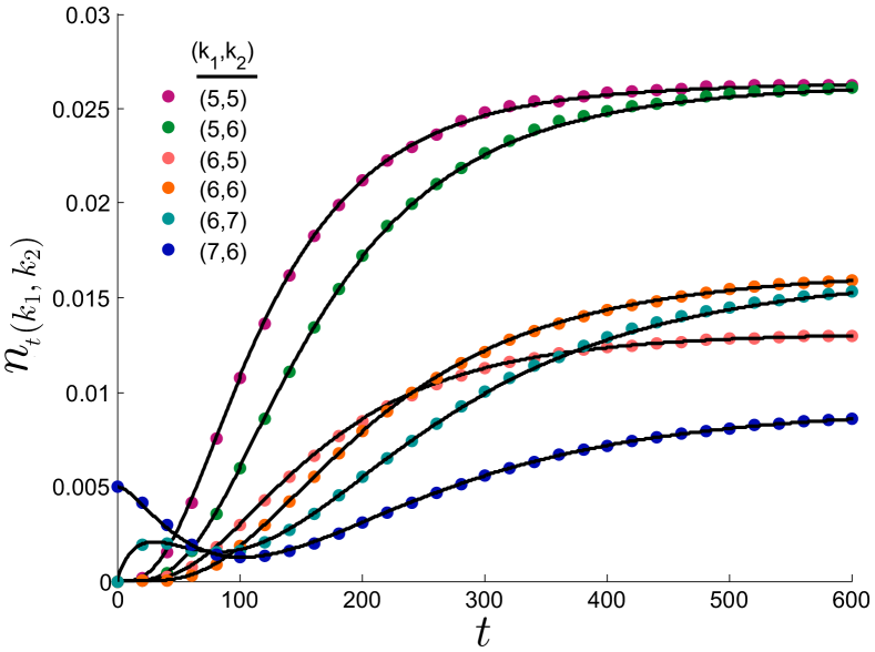
Figure 12: (Color online) Temporal evolution of the joint degree distribution for two layers. The initial networks are ${SW(200,0.05,2)}$ and ${SW(200,0.01,2)}$, respectively, as discussed in the text. The growth parameters are $\beta_{1}=3$ and $\beta_{2}=4$. Solid lines represent theoretical predictions, given in (66). Markers represent simulation results, averaged over 100 Monte Carlo trials.

We can also illustrate the evolution of the joint distribution by depicting it at different instants of time. To that end, since at most three dimensions can be plotted and $n_{t}(k_{1},k_{2})$ has four dimensions, we need to discard one dimension to enable us plot the distribution at different time points. To that end, we need to fix one dimension. Since the index of layers are arbitrary, without loss of generality, we fix $k_{1}$. For the simulation, consider the following setting. The initial network in layer 1 is a $SW(300,2,0.02)$ and that of layer 2 is $SW(300,4,0.04)$. The initial number of connections of incoming nodes are $\beta_{1}=4$ and $\beta_{2}=2$. We plot $n_{t}(k_{1},k_{2})$ at different time steps as a function of $k_{2}$, having fixed $k_{1}$ at the example value of $k_{1}=8$. In other words, we plot $n_{t}(8,k_{2})$. The results are depicted in Figure 13.

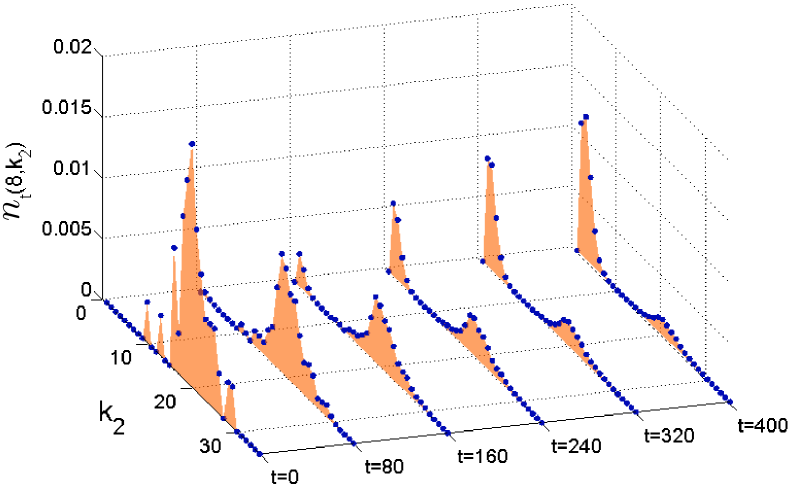
Figure 13: (Color online) The joint degree distribution $n_{t}(8,k_{2})$ as a function of $k_{2}$ for different times. The initial number of connections of incoming nodes are $\beta_{1}=4$ and $\beta_{2}=2$. The initial network in layer 1 is a $SW(300,2,0.02)$ and that of layer 2 is $SW(300,4,0.04)$. The shades represent theoretical predictions, given in (66). Markers represent simulation results, averaged over 100 Monte Carlo trials. Shades are chosen instead of linear plot for better visibility.

As another example, consider a ring with 100 nodes to be the initial network in the first layer, and let the nodes form an Erdős-Rényi (henceforth ER) network Erdös and Rényi (1960) in which the probability of existence of each link is 0.03. The results for the joint degree distribution with $k_{1}$ fixed at 2 is depicted in Figure 14. In other words, Figure 14 depicts $n_{t}(2,k_{2})$ as a function of $k_{2}$ at multiple instants of time. As time progresses, a peak at $k_{2}=\beta_{2}$ emerges. This is because as more new nodes enter the network, the number of newcomers who have degree $\beta_{2}$ increases and they constitute the majority of the network at long times. This causes the initial lump in Figure 14—which pertained to the initial network—to lose its mass and become smaller. The mass moves towards $k_{2}=\beta_{2}$ and construct a peak there.

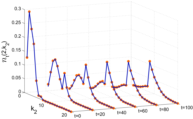
Figure 14: (Color online) The joint degree distribution $n_{t}(2,k_{2})$ as a function of $k_{2}$ at different instants of time (i.e., we have fixed $k_{1}=2$ to enable graphical illustration). The growth parameters are $\beta_{1}=2$ and $\beta_{2}=8$. The initial network in the first layer is a ring with 100 nodes, and in the second layer the topology is an ER network with the link existence probability equal to 0.03. The solid lines represent theoretical predictions, given in (66). Markers represent simulation results, averaged over 100 Monte Carlo trials. Note that as time progresses, a peak at $k_{2}=\beta_{2}$ emerges, which is intuitively expected.

For the next example, we consider two layers with Barabási-Albert (henceforth BA) topology Barabási and Albert (1999). The initial networks have 300 nodes, and the initial connectivity of incoming nodes are 2 for both layers. So in the resultant network, the majority of nodes have degree 2, and the degree distribution has a power-law tail with exponent 3, as is expected in BA graphs. After the BA network with 300 nodes has been constructed under the said mechanism, we start the growth process with growth parameters $\beta_{1}=1$ and $\beta_{2}=25$. This means that the second layer will be more densely connected as compared to layer 1. We fix the layer-1 degree at $k_{1}=3$ and plot ${n_{t}(3,k_{2})}$ as a function of $k_{2}$ at different instants of time. The results are presented in Figure 15. Note that the initial distribution has a peak at $k_{2}=2$, which is expected, because as mentioned above, the majority of nodes in the initial BA graph have degree 2 in both layers. As the growth process proceeds, the center of the peak moves towards higher values of $k_{2}$. This is because the newcomers have initial degree $\beta_{2}=25$ in the second layer, and as time progresses, the number of such nodes increase.

Figure 15: (Color online) The joint degree distribution $n_{t}(3,k_{2})$ as a function of $k_{2}$ at different instants of time (i.e., we have fixed $k_{1}=3$ to enable graphical illustration). The growth parameters are $\beta_{1}=1$ and $\beta_{2}=25$. The solid lines represent theoretical predictions, given in (66). Markers represent simulation results, averaged over 100 Monte Carlo trials. The initial networks are BA networks in both layers, as described in the text.

Let us also investigate the effect of sudden change in the growth parameters through one example. Consider a random recursive tree Dorogovtsev et al. (2008), which is constructed as follows. We begin by a single node, and then new nodes enter the system sequentially, and each newcomer randomly chooses one existing node and connects to it. The result is a tree, called a random recursive tree (hereinafter RRT). We choose the initial networks in both layers to be RRTs with 100 nodes. We then apply to this substrate a growth process with $\beta_{1}=1$ (which would be a continuation of the growth mechanism that gave rise to the RRT in the first layer) and $\beta_{2}=10$. This means that in the second layer, the growth mechanism is undergoing a regime shift, as the number of connections per incoming node abruptly jumps from 1 to 10. The results for the temporal evolution of ${n_{t}(1,k_{2})}$ is plotted in Figure 16. We observe that a new peak emerges at $k_{2}=10$, and the initial lump that peaked at $k_{2}=1$ at the outset gradually loses its mass to the new lump concentrated at $k_{2}=10$, which embodies the nodes that are introduced to the network in the second phase of the growth process.

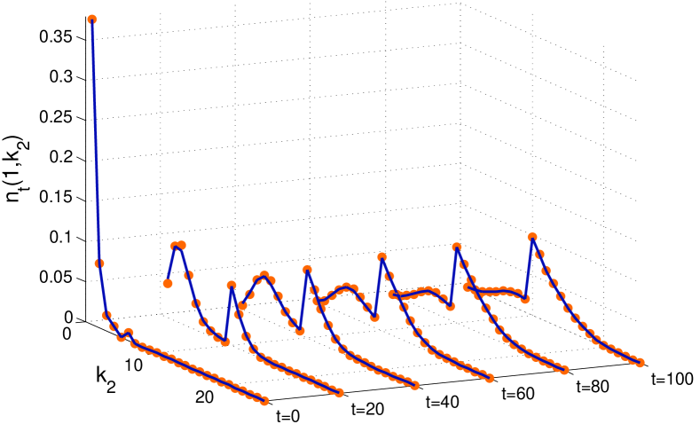
Figure 16: (Color online) The joint degree distribution $n_{t}(1,k_{2})$ as a function of $k_{2}$ at different instants of time (i.e., we have fixed $k_{1}=1$ to enable graphical illustration). The growth parameters are $\beta_{1}=1$ and $\beta_{2}=10$. The solid lines represent theoretical predictions, given in (66). Markers represent simulation results, averaged over 100 Monte Carlo trials. The initial networks are RRT networks in both layers, as described in the text.

Let us also consider one example to verify accuracy of the theoretical prediction of the joint degree distribution for more than two layers. Let us consider the following setting for the initial network: a BA network of 100 nodes with parameter 1 (that is, the initial number of links each incoming node establishes upon birth is 1) in the first layer, a BA network with parameter 2 in the second layer, and a BA network with parameter 3 in the third layer. For the growth mechanism, we consider $\beta_{1}=1$, $\beta_{2}=4$, and $\beta_{3}=5$. The results for several example triplets of $(k_{1},k_{2},k_{3})$ are depicted in Figure 17 . simulation results are visibly in good agreement with theoretical predictions.

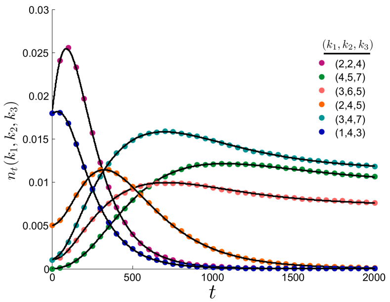
Figure 17: (Color online) The joint degree distribution $n_{t}(k_{1},k_{2},k_{3})$ for several example triplets $(k_{1},k_{2},k_{3})$. The growth parameters are $\beta_{1}=1$, $\beta_{2}=4$, and $\beta_{3}=5$. The solid lines represent theoretical predictions, and the markers represent simulation results averaged over 1000 Monte Carlo trials. The initial networks are BA networks in all three layers, as discussed in the text.

VII Summary and Open Problems

In this paper we focused on heterogeneous growth of multiplex networks. We considered both the preferential and uniform growth mechanisms. We analyzed the problem for $M>2$ layers and obtained the joint degree distributions. For the case of uniform growth, we analyzed the problem for arbitrary times, and obtained the joint degree distribution for arbitrary number of layers at arbitrary times, for given initial conditions. We verified our findings through Monte Carlo simulations, and observed that the theoretical predictions are remarkably accurate.

An immediate generalization of this work is to consider nonzero couplings in the preferential growth mechanism, so that the link reception probability of a node in each layer depends on its degrees in all layers, and then find the joint degree distribution via the rate equation approach (nonzero couplings are envisaged in Nicosia et al. (2013, 2014); Kim and Goh (2013), but the rate equation approach remains unsolved and no closed-form solution for the joint degree distribution exists in the literature). For example, in the two-layer case, the connection kernel would depend on the degrees of existing nodes in both layers. Consider an existing node $x$, who has degree $k_{x}$ in layer 1 and degree $\ell_{x}$ in layer 2 at time $t$. Then its probability of receiving a link in layer 1 from the incoming node would be proportional to $g_{11}k_{x}+g_{12}\ell_{x}$ , and its probability of receiving a link in layer 2 would be proportional to $g_{21}k_{x}+g_{22}\ell_{x}$. Our solution presented in this paper pertains to the special case of $g_{11}=g_{22}=1$ and $g_{12}=g_{21}=0$. The rate equation corresponding to the general case (counterpart of Equation (1), with all four $g_{ij}$s nonzero, would be as follows:

$$N_{k,\ell}(t+1)=N_{k,\ell}(t)+\delta_{k\beta_{1}}\delta_{\ell\beta_{2}}$$

$$+\beta_{1}\,\displaystyle\frac{\bigg{[}g_{11}(k-1)+g_{12}\ell\bigg{]}N_{t}(k-1,\ell)}{g_{11}L_{1}(0)+g_{12}L_{2}(0)+2(g_{11}\beta_{1}+g_{12}\beta_{2})t}$$

$$+\beta_{2}\,\displaystyle\frac{\bigg{[}g_{21}k+g_{22}(\ell-1)\bigg{]}N_{t}(k,\ell-1)}{g_{21}L_{1}(0)+g_{22}L_{2}(0)+2(g_{21}\beta_{1}+g_{22}\beta_{2})t}$$

$$-\beta_{1}\,\displaystyle\frac{\bigg{[}g_{11}k+g_{12}\ell\bigg{]}N_{k,\ell}(t)}{g_{11}L_{1}(0)+g_{12}L_{2}(0)+2(g_{11}\beta_{1}+g_{12}\beta_{2})t}$$

$$-\beta_{2}\,\displaystyle\frac{\bigg{[}g_{21}k+g_{22}\ell\bigg{]}N_{k,\ell}(t)}{g_{21}L_{1}(0)+g_{22}L_{2}(0)+2(g_{21}\beta_{1}+g_{22}\beta_{2})t}.$$ (67)

It is straightforward to simplify this equation in the steady state, but solving the resulting difference equation is more intricate than the one studied in this paper.

Furthermore, a related quantity which is ubiquitous in the studying of epidemics and various diffusion processes over networks is the nearest-neighbor degree distribution Eguiluz and Klemm (2002); Barthélemy et al. (2004); Castellano and Pastor-Satorras (2006, 2008). Let us denote this quantity by $p_{1}(k,\ell|q,r)$. For a node with degree $k$ in layer 1 and degree $\ell$ in layer 2, if we select one of its neighbors in layer 1 randomly, then $p_{1}(k,\ell|q,r)$ would be the probability that this neighbor has degree $q$ in layer 1 and degree $r$ in layer 2. Similarly, $p_{2}(k,\ell|q,r)$ would be the probability that a randomly selected layer-2 neighbor of a node with degrees $k,\ell$ will have degrees $q,r$. This quantity is essential for studying dynamics on networks, and to obtain it for multiplex networks, one also needs exact expressions for the degree distributions—which the present paper focused on.

Appendix A Solving Difference Equation (5)

We need to solve

$$n(k,\ell)= \,\displaystyle\frac{k-1}{k+\ell+2}n(k-1,\ell)\,\displaystyle\frac{\ell-1}{k+\ell+2}n(k,\ell-1)$$

$$+\,\displaystyle\frac{2\delta_{k\beta_{1}}\delta_{\ell\beta_{2}}}{2+\beta_{1}+\beta_{2}}.$$ (68)

We define the new sequence

$$m_{k\ell}\,\stackrel{{\scriptstyle\text{def}}}{{=}}\,\displaystyle\frac{(k+\ell+2)!}{(k-1)!(\ell-1)!}n(k,\ell).$$ (69)

The following holds

Plugging these into (68), we can recast it as

$$m_{k\ell}=m_{k-1,\ell}+m_{k,\ell-1}+2\,\displaystyle\frac{(\beta_{1}+\beta_{2}+1)!}{(\beta_{1}-1)!(\beta_{2}-1)!}\delta_{k,\beta_{1}}\delta_{\ell,\beta_{2}}.$$ (71)

Now define the Z-transform of sequence $m_{k,\ell}$ as follows:

$$\begin{cases}\psi(z,y)\,\stackrel{{\scriptstyle\text{def}}}{{=}}\,\displaystyle\sum_{k}\sum_{\ell}m_{k,\ell}z^{-k}y^{-\ell}\\ \\ m_{k,\ell}=\,\displaystyle\frac{1}{(2\pi i)^{2}}\,\displaystyle\oint\oint\psi(z,y)z^{k-1}y^{\ell-1}dzdy.\end{cases}$$ (72)

Taking the Z transform of every term in (71), we arrive at

$$\psi(z,y)= z^{-1}\psi(z,y)+y^{-1}\psi(z,y)$$

$$+2\,\displaystyle\frac{(\beta_{1}+\beta_{2}+1)!}{(\beta_{1}-1)!(\beta_{2}-1)!}z^{-\beta_{1}}y^{-\beta_{2}}.$$ (73)

This can be rearranged and rewritten as follows

$$\psi(z,y)=\,\displaystyle\frac{2}{1-z^{-1}-y^{-1}}\,\displaystyle\frac{(\beta_{1}+\beta_{2}+1)!}{(\beta_{1}-1)!(\beta_{2}-1)!}z^{-\beta_{1}}y^{-\beta_{2}}$$ (74)

The inverse transform is given by

$$m_{k,\ell}=\,\displaystyle\frac{2(\beta_{1}+\beta_{2}+1)!}{(\beta_{1}-1)!(\beta_{2}-1)!}\oint\oint\,\displaystyle\frac{z^{k-\beta_{1}-1}y^{\ell-\beta_{2}-1}dzdy}{(-4\pi^{2})(1-z^{-1}-y^{-1})}$$

$$=\,\displaystyle\frac{2(\beta_{1}+\beta_{2}+1)!}{(\beta_{1}-1)!(\beta_{2}-1)!}\oint\oint\,\displaystyle\frac{z^{k-\beta_{1}}y^{\ell-\beta_{2}}dzdy}{(-4\pi^{2})(zy-z-y)}$$

$$=\,\displaystyle\frac{2(\beta_{1}+\beta_{2}+1)!}{(\beta_{1}-1)!(\beta_{2}-1)!}\oint\oint\,\displaystyle\frac{z^{k-\beta_{1}}y^{\ell-\beta_{2}}dzdy}{(-4\pi^{2})(y-1)\big{[}z-\frac{y}{y-1}\big{]}}.$$ (75)

First we integrate over $z$. We get

$$m_{k,\ell} =\,\displaystyle\frac{2(\beta_{1}+\beta_{2}+1)!}{(\beta_{1}-1)!(\beta_{2}-1)!}\oint\,\displaystyle\frac{\left(\frac{y}{y-1}\right)^{k-\beta_{1}}y^{\ell-\beta_{2}}dy}{(2\pi i)(y-1)}$$

$$=\,\displaystyle\frac{2(\beta_{1}+\beta_{2}+1)!}{(\beta_{1}-1)!(\beta_{2}-1)!}\oint\,\displaystyle\frac{y^{k-\beta_{1}+\ell-\beta_{2}}dy}{(2\pi i)(y-1)^{k-\beta_{1}+1}}.$$ (76)

Now note that the residue of $\,\displaystyle\frac{f(y)}{(y-1)^{n}}$ for positive integer equals $\,\displaystyle\frac{f^{(n-1)}(1)}{(n-1)!}$, where the numerator denotes the ${(n-1)}$th derivative of the function $f(y)$, evaluated at ${y=1}$. Also, note that the $m$-th derivative of the function $y^{n}$, for integer $n$ and $m$, equals $\,\displaystyle\frac{m!}{(n-m)!}y^{n-m}$. Combining these two facts, we obtain

$$m_{k,\ell}=\,\displaystyle\frac{2(\beta_{1}+\beta_{2}+1)!}{(\beta_{1}-1)!(\beta_{2}-1)!}\,\binom{k-\beta_{1}+\ell-\beta_{2}}{k-\beta_{1}}.$$ (77)

Using (69), we arrive at

$$n(k,\ell)=\,\displaystyle\frac{2(\beta_{1}+\beta_{2}+1)!}{(\beta_{1}-1)!(\beta_{2}-1)!}\,\displaystyle\frac{1}{k(k+1)\ell(\ell+1)}\,\displaystyle\frac{\,\binom{k-\beta_{1}+\ell-\beta_{2}}{k-\beta_{1}}}{\,\binom{k+\ell+2}{k+1}}.$$ (78)

This can be equivalently expressed as follows:

(79)

Appendix B Performing the Summation in (8)

We need to calculate

$$\bar{\ell}(k)=\,\displaystyle\sum_{\ell}\frac{\beta_{2}(\beta_{2}+1)}{(2+\beta_{1}+\beta_{2})}\frac{\,\binom{\beta_{1}+\beta_{2}+2}{\beta_{1}+1}\,\binom{k-\beta_{1}+\ell-\beta_{2}}{k-\beta_{1}}}{\,\binom{k+\ell+2}{\ell}}$$ (80)

We use the following identity:

$$\,\displaystyle\frac{1}{\,\binom{n}{m}}=(n+1)\,\displaystyle\int_{0}^{1}t^{m}(1-t)^{n-m}dt,$$ (81)

to rewrite the binomial reciprocal of the coefficient as follows

$$\,\displaystyle\frac{1}{\,\binom{k+\ell+2}{\ell}}=(k+\ell+3)\,\displaystyle\int_{0}^{1}t^{\ell}(1-t)^{k+2}dt.$$ (82)

Also, from Taylor expansion, it is elementary to show that

$$S_{1}(x,n)\,\stackrel{{\scriptstyle\text{def}}}{{=}}\,\displaystyle\sum_{m}x^{m}\,\binom{m}{n}=\,\displaystyle\frac{x^{n}}{(1-x)^{n+1}}.$$ (83)

This identity will be used in the steps below.

Plugging (82) into (84), we have

$$\bar{\ell}(k) =\,\displaystyle\sum_{\ell}\frac{\beta_{2}(\beta_{2}+1)}{(2+\beta_{1}+\beta_{2})}\frac{\,\binom{\beta_{1}+\beta_{2}+2}{\beta_{1}+1}\,\binom{k-\beta_{1}+\ell-\beta_{2}}{k-\beta_{1}}}{\,\binom{k+\ell+2}{\ell}}$$

$$=\frac{\beta_{2}(\beta_{2}+1)}{(2+\beta_{1}+\beta_{2})}\,\binom{\beta_{1}+\beta_{2}+2}{\beta_{1}+1}\,\displaystyle\sum_{\ell}(k+\ell+3)\,\binom{k-\beta_{1}+\ell-\beta_{2}}{k-\beta_{1}}\,\displaystyle\int_{0}^{1}t^{\ell}(1-t)^{k+2}dt$$

$$=\frac{\beta_{2}(\beta_{2}+1)}{(2+\beta_{1}+\beta_{2})}\,\binom{\beta_{1}+\beta_{2}+2}{\beta_{1}+1}\,\displaystyle\int_{0}^{1}(1-t)^{k+2}t^{-k-2}\,\displaystyle\sum_{\ell}(k+\ell+3)t^{k+\ell+2}\,\binom{k-\beta_{1}+\ell-\beta_{2}}{k-\beta_{1}}dt$$

$$=\frac{\beta_{2}(\beta_{2}+1)}{(2+\beta_{1}+\beta_{2})}\,\binom{\beta_{1}+\beta_{2}+2}{\beta_{1}+1}\,\displaystyle\int_{0}^{1}(1-t)^{k+2}t^{-k-2}\,\displaystyle\frac{d}{dt}\left[\,\displaystyle\sum_{\ell}t^{k+\ell+3}\,\binom{k-\beta_{1}+\ell-\beta_{2}}{k-\beta_{1}}\right]dt$$

$$=\frac{\beta_{2}(\beta_{2}+1)}{(2+\beta_{1}+\beta_{2})}\,\binom{\beta_{1}+\beta_{2}+2}{\beta_{1}+1}\,\displaystyle\int_{0}^{1}(1-t)^{k+2}t^{-k-2}\,\displaystyle\frac{d}{dt}\left[t^{3+\beta_{1}+\beta_{2}}\,\displaystyle\sum_{\ell}t^{k-\beta_{1}+\ell-\beta_{2}}\,\binom{k-\beta_{1}+\ell-\beta_{2}}{k-\beta_{1}}\right]dt$$

$$\stackrel{{\scriptstyle\textnormal{\eqref{taylor_0}}}}{{=}}\frac{\beta_{2}(\beta_{2}+1)}{(2+\beta_{1}+\beta_{2})}\,\binom{\beta_{1}+\beta_{2}+2}{\beta_{1}+1}\,\displaystyle\int_{0}^{1}(1-t)^{k+2}t^{-k-2}\,\displaystyle\frac{d}{dt}\left[t^{3+\beta_{1}+\beta_{2}}\,\displaystyle\frac{t^{k-\beta_{1}}}{(1-t)^{k-\beta_{1}+1}}\right]dt$$

$$=\frac{\beta_{2}(\beta_{2}+1)}{(2+\beta_{1}+\beta_{2})}\,\binom{\beta_{1}+\beta_{2}+2}{\beta_{1}+1}\,\displaystyle\int_{0}^{1}(1-t)^{k+2}t^{-k-2}\,\displaystyle\frac{d}{dt}\left[\,\displaystyle\frac{t^{k+\beta_{2}+3}}{(1-t)^{k-\beta_{1}+1}}\right]dt$$

$$=\frac{\beta_{2}(\beta_{2}+1)}{(2+\beta_{1}+\beta_{2})}\,\binom{\beta_{1}+\beta_{2}+2}{\beta_{1}+1}\,\displaystyle\int_{0}^{1}(1-t)^{\beta_{1}}t^{\beta_{2}}\left[k+\beta_{2}+3-(1+\beta_{1}+\beta_{2})t\right]dt$$

$$=\frac{\beta_{2}(\beta_{2}+1)}{(2+\beta_{1}+\beta_{2})}\,\binom{\beta_{1}+\beta_{2}+2}{\beta_{1}+1}\left[(k+\beta_{2}+3)\,\displaystyle\int_{0}^{1}(1-t)^{\beta_{1}}t^{\beta_{2}}dt-(1+\beta_{1}+\beta_{2})\,\displaystyle\int_{0}^{1}(1-t)^{\beta_{1}}t^{\beta_{2}+1}dt\right]$$

$$\stackrel{{\scriptstyle\textnormal{\eqref{recip_binom}}}}{{=}}\frac{\beta_{2}(\beta_{2}+1)}{(2+\beta_{1}+\beta_{2})}\,\binom{\beta_{1}+\beta_{2}+2}{\beta_{1}+1}\left[(k+\beta_{2}+3)\,\displaystyle\frac{\beta_{1}!\beta_{2}!}{(\beta_{1}+\beta_{2}+1)!}-(1+\beta_{1}+\beta_{2})\,\displaystyle\frac{\beta_{1}!(\beta_{2}+1)!}{(\beta_{1}+\beta_{2}+2)!}\right]$$

$$=\frac{\beta_{2}(\beta_{2}+1)\beta_{1}!\beta_{2}!}{(2+\beta_{1}+\beta_{2})(1+\beta_{1}+\beta_{2})!}\,\binom{\beta_{1}+\beta_{2}+2}{\beta_{1}+1}\left[(k+\beta_{2}+3)-(\beta_{2}+1)\right]$$

$$=\,\displaystyle\frac{\beta_{2}}{\beta_{1}+1}(k+2)$$ (84)

Appendix C Proving the Identity Given in (11)

We use the property of the Gamma integral given in (81) in order to deal with the binomial coefficient that is in the denominator of the summand. We have:

$$\,\displaystyle\sum_{k}\,\displaystyle\frac{\,\binom{q-\beta_{1}-\beta_{2}}{k-\beta_{1}}}{\,\binom{q-2}{k-1}}$$

$$=\,\displaystyle\sum_{k}\,\binom{q-\beta_{1}-\beta_{2}}{k-\beta_{1}}(q-1)\int_{0}^{1}(1-t)^{k-1}t^{q-k-1}dt$$

$$=(q-1)\,\displaystyle\int_{0}^{1}t^{\beta_{2}-1}(1-t)^{\beta_{1}-1}$$

$$\stackrel{{\scriptstyle\textnormal{\eqref{iden_gamma}}}}{{=}}\,\displaystyle\frac{(q-1)}{(\beta_{2}+\beta_{1}-1)\,\binom{\beta_{2}+\beta_{1}-2}{\beta_{2}-1}}$$

$$=\,\displaystyle\frac{(\beta_{1}-1)!(\beta_{2}-1)!(q-1)}{(\beta_{2}+\beta_{1}-1)!}.$$ (85)

Appendix D Solving Difference Equation (16)

Let us repeat the equation we need to solve for easy reference

$$\leavevmode\resizebox{433.62pt}{}{$n(k,\ell)=\,\displaystyle\frac{\beta_{1}}{1+\beta_{1}+\beta_{2}}n(k-1,\ell)+\,\displaystyle\frac{\beta_{2}}{1+\beta_{1}+\beta_{2}}n_{k,\ell-1}+\,\displaystyle\frac{\delta_{k,\beta_{1}}\delta_{\ell,\beta_{2}}}{1+\beta_{1}+\beta_{2}}$}.$$ (86)

Let us define the following quantities from brevity:

$$\begin{cases}q_{1}&\,\stackrel{{\scriptstyle\text{def}}}{{=}}\,\displaystyle\frac{\beta_{1}}{1+\beta_{1}+\beta_{2}}\\ q_{2}&\,\stackrel{{\scriptstyle\text{def}}}{{=}}\,\displaystyle\frac{\beta_{2}}{1+\beta_{1}+\beta_{2}}\end{cases}$$ (87)

Taking the Z transform from both sides of (86), we get

$$\psi(z,y)=q_{1}z^{-1}\psi(z,y)+q_{2}y^{-1}\psi(z,y)+\,\displaystyle\frac{z^{-\beta_{1}}y^{-\beta_{2}}}{1+\beta_{1}+\beta_{2}}.$$ (88)

This can be rearranged and recast as

$$\psi(z,y)=\,\displaystyle\frac{1}{1-q_{1}z^{-1}-q_{2}y^{-1}}\,\displaystyle\frac{z^{-\beta_{1}}y^{-\beta_{2}}}{1+\beta_{1}+\beta_{2}}.$$ (89)

This can be inverted through the following steps

$$n(k,\ell) =\,\displaystyle\frac{1}{(1+\beta_{1}+\beta_{2})(2\pi i)^{2}}\,\displaystyle\oint\psi(z,y)z^{k-1}y^{\ell-1}dzdy$$

$$=\,\displaystyle\frac{1}{(1+\beta_{1}+\beta_{2})(2\pi i)^{2}}\,\displaystyle\oint\oint\,\displaystyle\frac{z^{k-\beta_{1}-1}y^{\ell-\beta_{2}-1}}{1-q_{1}z^{-1}-q_{2}y^{-1}}dzdy$$

$$=\,\displaystyle\frac{1}{(1+\beta_{1}+\beta_{2})(2\pi i)^{2}}\,\displaystyle\oint\oint\,\displaystyle\frac{z^{k-\beta_{1}}y^{\ell-\beta_{2}}}{zy-yq_{1}-zq_{2}}dzdy$$

$$=\,\displaystyle\frac{1}{(1+\beta_{1}+\beta_{2})(2\pi i)^{2}}\,\displaystyle\oint\oint\,\displaystyle\frac{z^{k-\beta_{1}}y^{\ell-\beta_{2}}}{z-\frac{yq_{1}}{y-q_{2}}}\,\displaystyle\frac{1}{y-q_{2}}dzdy$$

$$=\,\displaystyle\frac{1}{(1+\beta_{1}+\beta_{2})(2\pi i)}\,\displaystyle\oint\,\displaystyle\frac{y^{\ell-\beta_{2}}}{y-q_{2}}\left(\frac{yq_{1}}{y-q_{2}}\right)^{k-\beta_{1}}dzdy$$

$$=\,\displaystyle\frac{q_{1}^{k-\beta_{1}}}{(1+\beta_{1}+\beta_{2})(2\pi i)}\,\displaystyle\oint\,\displaystyle\frac{y^{k-\beta_{1}+\ell-\beta_{2}}}{(y-q_{2})^{k-\beta_{1}+1}}dzdy$$

$$=\,\displaystyle\frac{q_{1}^{k-\beta_{1}}}{(1+\beta_{1}+\beta_{2})}\,\displaystyle\,\displaystyle\frac{1}{(k-\beta_{1})!}\,\displaystyle\frac{(k-\beta_{1}+\ell-\beta_{2})!}{(\ell-\beta_{2})!}q_{2}^{\ell-\beta_{2}}$$

$$=\,\displaystyle\frac{q_{1}^{k-\beta_{1}}q_{2}^{\ell-\beta_{2}}}{(1+\beta_{1}+\beta_{2})}\,\binom{k-\beta_{1}+\ell-\beta_{2}}{k-\beta_{1}}.$$ (90)

After inserting the expressions for $q_{1},q_{2}$ from (87), this becomes

$$n(k,\ell)=\,\displaystyle\frac{\beta_{1}^{k-\beta_{1}}\beta_{2}^{\ell-\beta_{2}}\,\binom{k-\beta_{1}+\ell-\beta_{2}}{k-\beta_{1}}}{(1+\beta_{1}+\beta_{2})^{k-\beta_{1}+\ell-\beta_{2}+1}}.$$ (91)

Appendix E Performing the Summation in (19)

We need to perform the following summation:

$$\bar{\ell}(k) =\,\displaystyle\frac{(\beta_{1}+1)^{k-\beta_{1}+1}}{(\beta_{1}+\beta_{2}+1)^{k-\beta_{1}+1}}\,\displaystyle\sum_{\ell}\ell\frac{\beta_{2}^{\ell-\beta_{2}}\,\binom{k-\beta_{1}+\ell-\beta_{2}}{k-\beta_{1}}}{(1+\beta_{1}+\beta_{2})^{\ell-\beta_{2}}}$$ (92)

Let us denote $k-\beta_{1}$ by $k^{\prime}$ and $\ell-\beta_{2}$ by $\ell^{\prime}$. Also let us denote $\frac{\beta_{2}}{1+\beta_{1}+\beta_{2}}$ by $x$. De need to evaluate the following sum: ${\sum_{\ell^{\prime}}(\ell^{\prime}+\beta_{2})x^{\ell^{\prime}}\,\binom{k^{\prime}+\ell^{\prime}}{k^{\prime}}}$. Let us use (83) and define

$$S_{1}(x,n)\,\stackrel{{\scriptstyle\text{def}}}{{=}}\,\displaystyle\sum_{m}x^{m}\,\binom{m}{n}=\,\displaystyle\frac{x^{n}}{(1-x)^{n+1}}$$ (93)

We have:

$$\sum_{\ell^{\prime}}(\beta_{2}+\ell^{\prime})x^{\ell^{\prime}}\,\binom{k^{\prime}+\ell^{\prime}}{k^{\prime}}$$

$$=\beta_{2}x^{-k^{\prime}}S_{1}(x,k^{\prime})+x\sum_{\ell^{\prime}}\ell^{\prime}x^{\ell^{\prime}-1}\,\binom{k^{\prime}+\ell^{\prime}}{k^{\prime}}$$

$$=\beta_{2}x^{-k^{\prime}}S_{1}(x,k^{\prime})+x\,\displaystyle\frac{d}{dx}\Big{(}x^{-k^{\prime}}S_{1}(x,k^{\prime})\Big{)}$$

$$=\beta_{2}x^{-k^{\prime}}\,\displaystyle\frac{x^{k^{\prime}}}{(1-x)^{k^{\prime}+1}}+x\,\displaystyle\frac{d}{dx}\Big{(}\,\displaystyle\frac{x^{k^{\prime}}}{(1-x)^{k^{\prime}+1}}\Big{)}$$

$$=\,\displaystyle\frac{1}{(1-x)^{k^{\prime}+2}}\big{[}\beta_{2}+x(k^{\prime}+1-\beta_{2})\big{]}.$$ (94)

Replacing $x$ with $\frac{\beta_{2}}{1+\beta_{1}+\beta_{2}}$ and $k^{\prime}$ by $k-\beta_{1}$ and inserting this result into (92), we get

$$=\,\displaystyle\frac{(1+\beta_{1}+\beta_{2})^{k-\beta_{1}+2}}{(1+\beta_{1})^{k-\beta_{1}+2}}\big{[}\frac{\beta_{2}(k+2)}{1+\beta_{1}+\beta_{2}}\big{]}$$ (95)

Plugging this into (92), we get

$$\bar{\ell}(k) =\frac{\beta_{2}(k+2)}{1+\beta_{1}}$$ (96)

References

• Menichetti et al. (2014) G. Menichetti, D. Remondini, P. Panzarasa, R. J. Mondragón,  and G. Bianconi, PloS one 9, e97857 (2014).
• Nicosia and Latora (2014) V. Nicosia and V. Latora, arXiv preprint arXiv:1403.1546  (2014).
• Lewis et al. (2008) K. Lewis, J. Kaufman, M. Gonzalez, A. Wimmer,  and N. Christakis, Social networks 30, 330 (2008).
• Magnani and Rossi (2011) M. Magnani and L. Rossi, in Advances in Social Networks Analysis and Mining (ASONAM), 2011 International Conference on (IEEE, 2011) pp. 5–12.
• Bargigli et al. (2015) L. Bargigli, G. Di Iasio, L. Infante, F. Lillo,  and F. Pierobon, Quantitative Finance 15, 673 (2015).
• Cardillo et al. (2013) A. Cardillo, J. Gómez-Gardeñes, M. Zanin, M. Romance, D. Papo, F. del Pozo,  and S. Boccaletti, Sci. Rep. 3 (2013).
• Battiston et al. (2015a) F. Battiston, J. Iacovacci, V. Nicosia, G. Bianconi,  and V. Latora, arXiv preprint arXiv:1506.01280  (2015a).
• Szell et al. (2010) M. Szell, R. Lambiotte,  and S. Thurner, Proc. Nat. Acad. Sci. 107, 13636 (2010).
• De Domenico et al. (2013a) M. De Domenico, A. Solé-Ribalta, E. Cozzo, M. Kivelä, Y. Moreno, M. A. Porter, S. Gómez,  and A. Arenas, Phys. Rev. X 3, 041022 (2013a).
• Kivel’́a et al. (2014) M. Kivel’́a, A. Arenas, M. Barthelemy, J. P. Gleeson, Y. Moreno,  and M. A. Porter, J Complex Net. 2, 203 (2014).
• Sole-Ribalta et al. (2013) A. Sole-Ribalta, M. De Domenico, N. E. Kouvaris, A. Diaz-Guilera, S. Gomez,  and A. Arenas, Phy. Rev. E 88, 032807 (2013).
• Son et al. (2012) S.-W. Son, G. Bizhani, C. Christensen, P. Grassberger,  and M. Paczuski, Eur. Phy. Lett. 97, 16006 (2012).
• Saumell-Mendiola et al. (2012) A. Saumell-Mendiola, M. Á. Serrano,  and M. Boguñá, Phys. Rev. E 86, 026106 (2012).
• Granell et al. (2013) C. Granell, S. Gómez,  and A. Arenas, Phys. Rev. Lett. 111, 128701 (2013).
• Granell et al. (2014) C. Granell, S. Gómez,  and A. Arenas, Physical Review E 90, 012808 (2014).
• Cellai et al. (2013) D. Cellai, E. López, J. Zhou, J. P. Gleeson,  and G. Bianconi, Phys. Rev. E 88, 052811 (2013).
• Baxter et al. (2014) G. J. Baxter, S. N. Dorogovtsev, J. F. Mendes,  and D. Cellai, Phys. Rev. E 89, 042801 (2014).
• De Domenico et al. (2013b) M. De Domenico, A. Solé, S. Gómez,  and A. Arenas, arXiv preprint arXiv:1306.0519  (2013b).
• Battiston et al. (2015b) F. Battiston, V. Nicosia,  and V. Latora, arXiv preprint arXiv:1505.01378  (2015b).
• Matamalas et al. (2015) J. T. Matamalas, J. Poncela-Casasnovas, S. Gómez,  and A. Arenas, Scientific reports 5 (2015).
• Gómez-Gardeñes et al. (2012) J. Gómez-Gardeñes, I. Reinares, A. Arenas,  and L. M. Floría, Scientific reports 2 (2012).
• Wang et al. (2013) Z. Wang, A. Szolnoki,  and M. Perc, Sci. Rep. 3 (2013).
• Wang et al. (2015) Z. Wang, L. Wang, A. Szolnoki,  and M. Perc, The European Physical Journal B 88, 1 (2015).
• Gomez et al. (2013) S. Gomez, A. Diaz-Guilera, J. Gomez-Gardeñes, C. J. Perez-Vicente, Y. Moreno,  and A. Arenas, Phys. Rev. Lett. 110, 028701 (2013).
• Cozzo et al. (2013) E. Cozzo, R. A. Banos, S. Meloni,  and Y. Moreno, Phys. Rev. E 88, 050801 (2013).
• Boccaletti et al. (2014) S. Boccaletti, G. Bianconi, R. Criado, C. Del Genio, J. Gómez-Gardeñes, M. Romance, I. Sendiña-Nadal, Z. Wang,  and M. Zanin, Phys. Rep. 544, 1 (2014).
• Kenett et al. (2015) D. Y. Kenett, M. Perc,  and S. Boccaletti, Chaos, Solitons & Fractals 80, 1 (2015).
• Nicosia et al. (2014) V. Nicosia, G. Bianconi, V. Latora,  and M. Barthelemy, Phys. Rev. E 90, 042807 (2014).
• Nicosia et al. (2013) V. Nicosia, G. Bianconi, V. Latora,  and M. Barthelemy, Phys. Rev. Lett. 111, 058701 (2013).
• Kim and Goh (2013) J. Y. Kim and K.-I. Goh, Phys. Rev. Lett. 111, 058702 (2013).
• Bianconi (2015) G. Bianconi, Phys. Rev. E 91, 012810 (2015).
• Fotouhi and Momeni (2015) B. Fotouhi and N. Momeni, in Complex Networks VI (Springer, 2015) pp. 159–170.
• Halu et al. (2014) A. Halu, S. Mukherjee,  and G. Bianconi, Physical Review E 89, 012806 (2014).
• Barigozzi et al. (2010) M. Barigozzi, G. Fagiolo,  and D. Garlaschelli, Physical Review E 81, 046104 (2010).
• Dorogovtsev et al. (2000) S. N. Dorogovtsev, J. F. F. Mendes,  and A. N. Samukhin, Phys. Rev. Lett. 85, 4633 (2000).
• Krapivsky et al. (2000) P. Krapivsky, S. Redner,  and F. Leyvraz, Phys. Rev. Lett. 85, 4629 (2000).
• Fotouhi and Rabbat (2013) B. Fotouhi and M. G. Rabbat, Physical Review E 88, 062801 (2013).
• Boyce et al. (1992) W. E. Boyce, R. C. DiPrima,  and C. W. Haines, Elementary differential equations and boundary value problems, Vol. 9 (Wiley New York, 1992).
• Newman and Watts (1999) M. E. Newman and D. J. Watts, Physics Letters A 263, 341 (1999).
• Erdös and Rényi (1960) P. Erdös and A. Rényi, Publ. Math. Inst. Hung. Acad. Sci 5, 17 (1960).
• Barabási and Albert (1999) A.-L. Barabási and R. Albert, science 286, 509 (1999).
• Dorogovtsev et al. (2008) S. N. Dorogovtsev, P. L. Krapivsky,  and J. Mendes, EPL (Europhysics Letters) 81, 30004 (2008).
• Eguiluz and Klemm (2002) V. M. Eguiluz and K. Klemm, Phys. Rev. Lett. 89, 108701 (2002).
• Barthélemy et al. (2004) M. Barthélemy, A. Barrat, R. Pastor-Satorras,  and A. Vespignani, Phys. Rev. Lett. 92, 178701 (2004).
• Castellano and Pastor-Satorras (2006) C. Castellano and R. Pastor-Satorras, Phys. Rev. Lett. 96, 038701 (2006).
• Castellano and Pastor-Satorras (2008) C. Castellano and R. Pastor-Satorras, Phys. Rev. Lett. 100, 148701 (2008).