Competitive Selection of Ephemeral Relays in Wireless Networks

Abstract

We consider a setting in which two nodes (referred to as forwarders) compete to choose a relay node from a set of relays, as they ephemerally become available (e.g., wake up from a sleep state). Each relay, when it arrives, offers a (possibly different) “reward” to each forwarder. Each forwarder’s objective is to minimize a combination of the delay incurred in choosing a relay and the reward offered by the chosen relay. As an example, we develop the reward structure for the specific problem of geographical forwarding over a network of sleep-wake cycling relays.

We study two variants of the generic relay selection problem, namely, the completely observable (CO) case where, when a relay arrives, both forwarders get to observe both rewards, and the partially observable (PO) case where each forwarder can only observe its own reward. Formulating the problem as a two person stochastic game, we characterize solution in terms of Nash Equilibrium Policy Pairs (NEPPs). For the CO case we provide a general structure of the NEPPs. For the PO case we prove that there exists an NEPP within the class of threshold policy pairs.

We then consider the particular application of geographical forwarding of packets in a shared network of sleep-wake cycling wireless relays. For this problem, for a particular reward structure, using realistic parameter values corresponding to TelosB wireless mote, we numerically compare the performance (in terms of cost to both forwarders) of the various NEPPs and draw the following key insight: even for moderate separation between the two forwarders, the performance of the various NEPPs is close to the performance of a simple strategy where each forwarder behaves as if the other forwarder is not present. We also conduct simulation experiments to study the end-to-end performance of the simple forwarding policy.

I Introduction

We are concerned in this paper with a class of resource allocation problems in wireless networks, in which competing nodes need to acquire a resource, such as a physical radio relay (see the geographical forwarding example later in Section III) or a channel (as in a cognitive radio network [1, 2]), when a sequence of such resources “arrive” over time, and are available only fleetingly for acquisition. In this paper, formulating such a problem for two nodes as a stochastic game, we consider the completely observable and partially observable cases, and provide characterizations of the Nash Equilibrium Policy Pairs (NEPP). We provide numerical results, and insights therefrom, for a specific reward structure derived from the problem of geographical forwarding in sleep-wake cycling networks.

The Geographical Forwarding Context: With the increasing importance of “smart” utilization of our limited resources (e.g., energy and clean water) there is a need for instrumenting our buildings and campuses with wireless sensor networks. As awareness grows and sensing technologies emerge, new applications will be implemented. While each application will require different sensors and back-end analytics, the availability of a common wireless network infrastructure will promote the quick deployment of new applications. One approach for building such an infrastructure, say, in a large building setting, would be to deploy a large number of relay nodes, and employ the idea of geographical forwarding. If the phenomena to be monitored are slowly varying over time, the traffic on the network can be assumed to be light. In addition, such applications are delay tolerant, thus accommodating the approach of opportunistic geographical forwarding over sleep-wake cycling networks [3, 4].

Sleep-wake cycling is an approach whereby, to conserve the relay battery power, their radios are kept turned OFF, while coming ON periodically to provide opportunities for packet forwarding. The problem of forwarding in such a setting was explored in [3, 4], where the formulation was limited to a single alarm packet flowing through the network. Whereas the emphasis in [3] was to develop an end-to-end optimal forwarding algorithm, thus requiring a global organization step, in [4], which is our prior work on this problem, we sought a locally-optimal forwarding heuristic. End-to-end forwarding was achieved by applying the local heuristic at each forwarding step. We found that, over certain range of operation, the performance obtained by the heuristic is comparable with the optimal solution provided by [3].

In the setting discussed above, even though the traffic is light, there is still a chance that there is more than one forwarder seeking a relay from among a set of potential relays. There then arises the problem of assigning the relays, as they wake-up, to one or the other of the forwarders. This, thus, is an extension of the local forwarding problem discussed in [4]. Formally, the local forwarding problem we consider in this paper is the following. There are two forwarders each of which has to choose a relay node to forward its packet to. The relays are waking up sequentially over time. Whenever a relay wakes up, each forwarder first evaluates the relay based on a reward metric (which could be a function of the progress, towards the sink, made by the relay, and the power required to get the packet to the relay [4]), and then decides whether to compete (with the other forwarder) for this relay or continue to wait for further relays to wake-up. Such a geographical forwarding setting will serve as an example application of the stochastic game formulation developed in this paper.

Outline and Our Contributions: We will describe a general system model in Section II, following which, in Section III, we will discuss a geographical forwarding problem as an example. Related work will be presented in Section IV. In Sections V and VI we will study two variants of the problem (of progressive complexity), namely, one where complete information is available to both forwarders and one with only partial information. We will use stochastic game theory to obtain solution in terms of (stationary) Nash Equilibrium Policy Pairs (NEPPs). We will briefly study a cooperative setting in Section VII, and obtain the Pareto optimal performance curve which provides a benchmark for the NEPPs. The following are our main technical contributions:

• For the problem with complete information we obtain results illustrating the structure of NEPPs (Theorem 2)

• For the partial information case we prove the existence of a NE strategy (for a certain Bayesian game) within the class of threshold strategies (Theorem 4). This result will enable us to construct NEPPs for this case.

• In Section VIII we provide a simulation study of the use of our formulation in the context of geographical forwarding. Using realistic parameters from the popular TelosB wireless mote, we make the following interesting observation: even for moderate separation between the two forwarders, the performance of all the NEPPs is close to the performance of a simple strategy where each forwarder behaves as if it is alone.

We will finally draw our conclusions in Section IX. For the ease of presentation we have moved most of the proofs to the Appendix.

II System Model

Let $\mathscr{F}_{1}$ and $\mathscr{F}_{2}$ denote the two competing nodes (i.e., players in game theoretic terms), referred to as the forwarders. We will assume that there are an infinite number of relay nodes (or resources in general) that are arriving sequentially at times $\{W_{k}:k\geq 0\}$, which are the points of a Poisson process of rate $\frac{1}{\tau}$. Thus, the inter-“arrival” times between successive relays, $U_{k}:=W_{k}-W_{k-1}$, are i.i.d. (independent and identically distributed) exponential random variables of mean $\tau$. We will refer to the relay that arrives at the instant $W_{k}$ as the $k$-th relay. Further, the $k$-th relay is only ephemerally available at the instant $W_{k}$.

When a relay arrives, either of the forwarders can compete for it, thereby obtaining a reward. Let $R_{\rho,k}$, $\rho=1,2$, denote the reward offered by the $k$-th relay to $\mathscr{F}_{\rho}$ (an example reward structure will be discussed in Section III). The rewards $R_{\rho,k}$ ($\rho=1,2$; $k\geq 1$) can take values from a finite set $\mathcal{R}=\{r_{1},r_{2},\cdots,r_{n}\}$, where $r_{1}=-\infty$ and $r_{i}<r_{j}$ for $i<j$. The reward pairs $(R_{1,k},R_{2,k})$ are i.i.d. across $k$, with their common joint p.m.f. (probability mass function) being $p_{R_{1},R_{2}}(\cdot,\cdot)$, For notational simplicity we will denote $p_{R_{1},R_{2}}(r_{i},r_{j})$ as simply $p_{i,j}$. Further, let $p^{(1)}_{i}$ and $p^{(2)}_{j}$ denote the marginal p.m.f.s of $R_{1,k}$ and $R_{2,k}$, respectively. Thus, $p^{(1)}_{i}=\sum_{j=1}^{n}p_{i,j}$ and $p^{(2)}_{j}=\sum_{i=1}^{n}p_{i,j}$.

Actions and Consequences: First we will study (in Section V) a completely observable case where the reward pair $(R_{1,k},R_{2,k})$ is revealed to both the forwarders. Later, in Section VI, we will consider a more involved (albeit more practical) partially observable case where only $R_{1,k}$ is revealed to $\mathscr{F}_{1}$, and $R_{2,k}$ is revealed to $\mathscr{F}_{2}$. However in either case, each time a relay arrives, the two forwarders have to independently choose between one of the following actions:

• s: stop and forward the packet to the current relay, or

• c: continue to wait for further relays to arrive.

Suppose both forwarders choose to stop, then with probability (w.p.) $\nu_{1}$, $\mathscr{F}_{1}$ gets the relay in which case $\mathscr{F}_{2}$ has to continue alone, while with the remaining probability ($\nu_{2}=1-\nu_{1}$) $\mathscr{F}_{2}$ gets the relay and $\mathscr{F}_{1}$ continues alone. $\nu_{\rho}$ ($\rho=1,2$) could be thought of as the probability that $\mathscr{F}_{\rho}$ will win the contention when both forwarders attempt simultaneously. For mathematical tractability we will assume that the forwarders make their decision instantaneously at the relay arrival instants. Further, if a relay is not chosen by either forwarder (i.e., if both forwarders choose to continue) we will assume that the relay disappears and is not available for further use.

System State and Forwarding Policy: For the CO case, $(R_{1,k},R_{2,k})$ can be regarded as the state of the system at stage $k$, provided both forwarders have not terminated (i.e., chosen a relay) yet. When one of the forwarder, say $\mathscr{F}_{2}$, terminates, we will represent the system state as $(R_{1,k},\textbf{\emph{t}})$. Similarly, let $(\textbf{\emph{t}},R_{2,k})$ and $(\textbf{\emph{t}},\textbf{\emph{t}})$ represents the state of the system when only $\mathscr{F}_{1}$ has terminated and when both forwarders have terminated, respectively. Formally, we can define the state space to be

$$\mathcal{X}=\Big{\{}(r_{i},r_{j}),(r_{i},\textbf{\emph{t}}),(\textbf{\emph{t}},r_{j}),(\textbf{\emph{t}},\textbf{\emph{t}}):r_{i},r_{j}\in\mathcal{R}\Big{\}}.$$ (1)

Given a discrete set $\mathcal{S}$, let $\Delta(\mathcal{S})$ denote the set of all p.m.f.s on $\mathcal{S}$. We now have the following definition.

Definition 1

A forwarding policy $\pi$ is a mapping, $\pi:\mathcal{X}\rightarrow\Delta(\{\mbox{{s},{c}}\})$, such that $\mathscr{F}_{1}$ (or $\mathscr{F}_{2}$) using $\pi$ will choose action s or c according to the p.m.f.  $\pi(x_{k})$ when the state of the system at stage $k\geq 1$ is $x_{k}\in\mathcal{X}$. A policy pair $(\pi_{1},\pi_{2})$ is a tuple of policies such that $\mathscr{F}_{1}$ uses $\pi_{1}$ and $\mathscr{F}_{2}$ uses $\pi_{2}$.

Note that we have restricted to the class of stationary policies only. We will denote this class of policies as $\Pi_{S}$.

Problem Formulation: Suppose the forwarders use a policy pair $(\pi_{1},\pi_{2})$, and let $x\in\mathcal{X}$ be the state of the system at stage $1$. Let $K_{\rho}$, $\rho=1,2$, denote the (random) stage at which $\mathscr{F}_{\rho}$ forwards its packet. Then, the delay incurred by $\mathscr{F}_{\rho}$ ($\rho=1,2$), starting from the instant $W_{1}=U_{1}$ (first relay’s arrival instant), is $D_{K_{\rho}}=U_{2}+\cdots+U_{K_{\rho}}$, and the reward accrued is $R_{\rho,K_{\rho}}$. Let $\mathbb{E}_{\pi_{1},\pi_{2}}^{x}[\cdot]$ denote the expectation operator corresponding to the probability law, $\mathbb{P}_{\pi_{1},\pi_{2}}^{x}$, governing the system dynamics when the policy pair used is $(\pi_{1},\pi_{2})$ and the initial state is $x$. Then, the expected total cost incurred by $\mathscr{F}_{\rho}$ is

$$J^{(\rho)}_{\pi_{1},\pi_{2}}(x)=\mathbb{E}_{\pi_{1},\pi_{2}}^{x}\Big{[}D_{K_{\rho}}-\eta_{\rho}R_{\rho,K_{\rho}}\Big{]},$$ (2)

where $\eta_{\rho}>0$ is the multiplier used to trade-off between delay and reward.

Definition 2

We say that a policy pair $(\pi_{1}^{*},\pi_{2}^{*})$ is a Nash equilibrium policy pair (NEPP) if, for all $x\in\mathcal{X}$, $J^{(1)}_{\pi_{1}^{*},\pi_{2}^{*}}(x)\leq J^{(1)}_{\pi_{1},\pi_{2}^{*}}(x)$ for any policy $\pi_{1}\in\Pi_{S}$, and $J^{(2)}_{\pi_{1}^{*},\pi_{2}^{*}}(x)\leq J^{(2)}_{\pi_{1}^{*},\pi_{2}}(x)$ for any policy $\pi_{2}\in\Pi_{S}$. Thus, a unilateral deviation from an NEPP is neither beneficial for $\mathscr{F}_{1}$ nor for $\mathscr{F}_{2}$.

Our objective will be to characterize the solution in terms of NEPPs.

III Geographical Forwarding Example

Before proceeding further, in this section, as a motivating example, we will construct a reward structure corresponding to the problem of geographical forwarding in sleep-wake cycling wireless networks. Let $\mathscr{F}_{1}$ and $\mathscr{F}_{2}$ actually represent two forwarding nodes in a wireless network. As shown in Fig. 1, let $v_{1}$ and $v_{2}$ denote their respective locations. A sink node is located at $v_{0}$. Let $d$ denote the range of both the forwarders. Given any location $\ell\in\Re^{2}$, we define the progress, $Z_{\rho}(\ell)$, made by location $\ell$ with respect to (w.r.t.) $\mathscr{F}_{\rho}$ as

$$Z_{\rho}(\ell) = \parallel v_{\rho}-v_{0}\parallel-\parallel\ell-v_{0}\parallel$$ (3)

where $\parallel\cdot\parallel$ denotes the Euclidean norm. Thus, $Z_{\rho}(\ell)$ is simply the difference between $\mathscr{F}_{\rho}$-to-sink and $\ell$-to-sink distances. A positive value of $Z_{\rho}(\ell)$ implies that location $\ell$ is closer to the sink than $\mathscr{F}_{\rho}$. Now, define the forwarding region, $\mathcal{L}_{\rho}$, of $\mathscr{F}_{\rho}$ as the set of all locations that lie within the range of $\mathscr{F}_{\rho}$ and make non-negative progress w.r.t. $\mathscr{F}_{\rho}$, i.e., denoting $D_{\rho}(\ell)=\parallel\ell-v_{\rho}\parallel$ to be the distance between $\ell$ and $\mathscr{F}_{\rho}$,

$$\mathcal{L}_{\rho} = \Big{\{}\ell:D_{\rho}(\ell)\leq d,Z_{\rho}(\ell)\geq 0\Big{\}}.$$ (4)

Let $\mathcal{L}=\mathcal{L}_{1}\cup\mathcal{L}_{2}$ denote the combined forwarding region of the two forwarders. As depicted in Fig. 1, we will discretize $\mathcal{L}$ into a grid of finite set of $m$ locations $\{\ell_{1},\ell_{2},\cdots,\ell_{m}\}$. Thus, from here on, whenever we refer to a location $\ell$ we mean it to be one of the above $m$ locations.

Sleep-Wake Process: Without loss of generality, we will assume that at time $0$ each forwarder is holding an alarm packet which has to forwarded to a downstream relay node (i.e., a node in its forwarding region). Since the relays are sleep-wake cycling, each forwarder has to wait until a “good” relay wakes up (the goodness of a relay will be based on the reward metric to be discussed in this section).

A practical approach for sleep-wake cycling is the asynchronous periodic sleep-wake process [3, 4], where each relay $i$ wakes up at the periodic instants $\{T_{i}+kT:k\geq 0\}$ with $\{T_{i}\}$ being i.i.d. (independent and identically distributed) uniform on $[0,T]$ ($T$ is referred to as the sleep-wake cycling period). Now, for dense networks where $N$ is large, if $T$ scales with $N$ such that $\frac{N}{T}=\frac{1}{\tau}$ as $N\rightarrow\infty$, then the aggregate point process of relay wake-up instants converges to a Poisson process of rate $\frac{1}{\tau}$ [7]. This observation motivates us to model the aggregate point process of wake-up instants of relays as a Poisson point process. Furthermore, the Poisson point process assumption renders our problem analytically tractable, leading to interesting structural results.

Thus, formally, we model the sleep-wake cycling by assuming that there are an infinite number of relays waking up (within the combined forwarding region $\mathcal{L}$) sequentially at the times $\{W_{k}:k\geq 0\}$ which are the points of a Poisson process of rate $\frac{1}{\tau}$ (thus, a new relay wakes up at each instant $W_{k}$). Let $L_{k}\in\mathcal{L}$ denote the location of the $k$-th relay (i.e., the relay waking up at the instant $W_{k}$). The locations $\{L_{k}:k\geq 1\}$ are i.i.d. random variables with their common p.m.f. (probability mass function) being $q$, i.e., $\mathbb{P}(L_{k}=\ell)=q_{\ell}$.

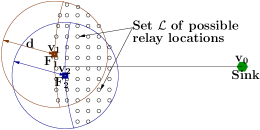
Figure 1: One-hop forwarding scenario: $v_{0}$, $v_{1}$, and $v_{2}$ are the locations of the sink, $\mathscr{F}_{1}$, and $\mathscr{F}_{2}$, respectively; $d$ is the range of each forwarder. Possible relay locations are shown as $\circ$.

Channel Model: We will use the following standard model to obtain the transmission power required by $\mathscr{F}_{\rho}$ to achieve an SNR (signal to noise ratio) constraint of $\Gamma$ at the $k$-th relay:

$$P_{\rho,k}=\frac{\Gamma N_{0}}{G_{\rho,k}}{\left(\frac{D_{\rho}(L_{k})}{d_{ref}}\right)}^{\xi}$$ (5)

where, $N_{0}$ is the receiver noise variance, $D_{\rho}(L_{k})$ is the distance between $\mathscr{F}_{\rho}$ and the $k$-th relay whose location is $L_{k}$, $G_{\rho,k}$ is the gain of the channel between $\mathscr{F}_{\rho}$ and the $k$-th relay, $\xi$ is the path-loss attenuation factor, and $d_{ref}$ is the far-field reference distance beyond which the above expression is valid [8, 9] (our discretization of $\mathcal{L}$ is such that the distance between $\mathscr{F}_{\rho}$ and any $\ell\in\mathcal{L}$ is more than $d_{ref}$).

We will assume that the set of channel gains $\{G_{\rho,k}:k\geq 1,\rho=1,2\}$ are i.i.d. taking values from a finite set $\mathcal{G}$. Also, let $P_{max}$ denote the maximum transmit power with which the two forwarders can transmit, i.e., if $P_{\rho,k}>P_{max}$ then $\mathscr{F}_{\rho}$ cannot forward its packet to the $k$-th relay. Further, we assume that the range $d$ (recall Fig. 1) is such that if the $k$-th relay is outside the range of $\mathscr{F}_{\rho}$ (i.e., $D_{\rho}(L_{k})>d$), then for any $G_{\rho,k}\in\mathcal{G}$, $P_{\rho,k}>P_{max}$, so that $\mathscr{F}_{\rho}$ cannot forward to a relay outside its range. Transmitting to a relay inside its range is possible, however, provided the channel gain is good enough so that the power required is less than $P_{max}$.

Relay Rewards: Finally, combining progress and power, we will define the reward offered by the $k$-th relay to $\mathscr{F}_{\rho}$ as,

$$R_{\rho,k} = \left\{\begin{array}[]{ll}\frac{{Z_{\rho}(L_{k})}^{a}}{P_{\rho,k}^{(1-a)}}&\mbox{ if }P_{\rho,k}\leq P_{max}\\ -\infty&\mbox{ otherwise, }\end{array}\right.$$ (8)

where $a\in[0,1]$ is the parameter used to trade-off between progress and power. The reward being inversely proportional to power is clear because it is advantageous to use low power to get the packet across; $R_{\rho,k}$ is made proportional to $Z_{\rho}(L_{k})$ to promote progress towards the sink while choosing a relay for the next hop.

We will use the above reward structure for conducting numerical and simulation experiments in Section VIII. However, it is important to note that all our analysis in the subsequent sections hold for the general model introduced in Section II.

IV Related Work

We will first make an important comparison with our prior work on the topic, before proceeding to discuss general literature from the area of geographical forwarding in wireless networks. Our problem can also be considered as a variant of the asset selling problem studied in the operations research literature; we will discuss related work from this field as well. Finally, we survey literature from the area of stochastic games.

Our Prior Work: Problem of relay selection, but by a single forwarder (i.e., the non-competitive version), has been extensively studied by us, starting from a simple model where the number of relays is exactly known to the forwarder to the one where only a belief is known [4]. We have also studied a variant with channel probing where the relay rewards are not immediately revealed to the forwarder; instead the forwarder can choose to learn the reward values by paying an additional cost [10].

The basic version of our model [4, Section 6] comprises only one forwarder and a finite number of relay $N$; however, in the basic model we allow for the forwarder to recall a previous relay unlike here where recalling is not allowed. For this basic model, the solution is completely in terms of a single threshold $\alpha$: forward to the first relay whose reward is more than $\alpha$; at the last stage choose the best relay irrespective of its reward value. From [4, Section 6], we further know that the value of $\alpha$ does not dependent on $N$, and hence the solution to the version of the basic model with infinite number of relays, should still be same. Furthermore, in the infinite horizon model there is no advantage in recalling the best relay since there is no last stage. Thus, one can argue that the solution to the infinite horizon basic relay selection model, without recall, should also be characterized by the same threshold $\alpha$. Here, we will formally show that this is in fact the solution for one forwarder when the other forwarder has already terminated (Lemma 1). However when both the forwarders are present, the solution is more involved (studied in Section 1). Thus, the competitive model studied here is a generalization of the aforementioned version of the basic relay selection model.

Geographical Forwarding: The problem of choosing a next-hop relay arises in the context of geographical forwarding; geographical forwarding [5, 6] is a forwarding technique where the prerequisite is that the nodes know their respective locations as well as the sink’s location. The method of geographical forwarding was already envisioned in the 80’s in the context of routing in packet radio networks (PRNs) [11, 12]. One of the simplest geographical forwarding technique is the greedy algorithm where each node forwards to a neighbor in its communication region which makes maximum progress towards the sink. This greedy algorithm is referred to as the MFR (Max Forward within Radius) routing in [11]. Akin to MFR is the NFP (Nearest with Forward Progress) proposed in [12] where a node with a positive progress, and closest to the transmitting node is chosen. A generalization of MFR and NFP routing is to randomly choose any neighbor which makes a positive progress towards the sink [13].

More recently, there are work that apply geographical forwarding for routing in sleep-wake cycling networks. For instance, Zorzi and Rao in [14] propose an algorithm called GeRaF (Geographical Random Forwarding) which, at each forwarding stage, chooses the relay making the largest progress. For a sleep-wake cycling network, Liu et al. in [15] propose a relay selection approach as a part of CMAC, a protocol for geographical packet forwarding. Under CMAC, node $i$ chooses an $r_{0}$ that minimizes the expected normalized latency (which is the average ratio of one-hop delay and progress). Akin to the relay selection problem is the problem of channel selection [16, 17] where a transmitter, given several channels, has to choose one for its transmissions. Analogous to rewards in our case, the transmitter’s decision is based on the throughput the transmitter can achieve on a channel. Links to more literature on similar work from the context of wireless networks can be found in [4]. However all these work do not consider the competitive scenario like ours.

Asset Selling Problem: Finally, our relay selection problem can be considered to be equivalent to the asset selling problem, which is a class of the optimal stopping problems studied in the operations research literature (other examples of stopping problems include the secretary problem [18], bandit problem [19], etc). The basic asset selling problem [20, Section 4.4] [21] comprises a single seller (analogous to a forwarder in our model) and a sequence of i.i.d. offers (rewards in our case). The seller’s objective is to choose an offer so as to maximize a combination of the offer value and the number of previous offers rejected. Over the years, several variants of the basic problem have been studied. For instance, In [22], David and Levi consider a model in which the offers arrive at the points of a renewal process. Kang in [23] has considered a model where a cost has to be paid to recall the previous best offer; see [23] for further references to literature on models with uncertain recall. Variants with unknown offer (or reward) distribution, or one where a parameter of the offer distribution is unknown have been studied in [24, 25].

Our competitive model here can be considered as a game variant of the basic asset selling problem, where the two forwarders are analogous to the sellers and the reward values are analogous to the offers. Although one game variant has been studied by Nakagami in [26], the specific cost structure in our problem enables us to prove results such as the existence of Nash equilibrium policy pair within the class of threshold rules (Theorem 4). Further, we also study a completely observable case which is not considered in [26].

Similarly, literature is available on the game version of the secretary problem [27, 28], but these consider the simpler case where the reward offered by an arriving secretary (or resource) to both players is the same. Moreover, the objective in the secretary problem is to maximize the probability of choosing the best secretary (resource), which is in contrast to our setting (asset selling) which involves a trade-off between selection delay and reward. Further, a partially observable scenario is not studied in these work.

Stochastic Games: Stochastic games can be considered as a generalization of Markov decision processes (MDPs), in the sense that a stochastic game comprises multiple agents (in contrast to a single agent in an MDP), who jointly control the state of the system while individually incurring a cost in doing so. Several references [29, 30, 31, 32, 33, 34] are available on the topic starting from the seminal work by Shapley [35]. However, most of these work study either discounted or average cost objectives, unlike our problem which falls within the realm of total-cost transient stochastic games (or stopping games [36, Part III]). Our formulation can be alternatively thought of as a quitting game [37]. However, we have introduced state transitions and state dependent quitting cost which are not considered in the model studied in [37].

In summary, to the best of our knowledge, the model proposed in this paper along with the structural results we have derived, are new contributions to the field of stopping games.

V Completely Observable (CO) Case

For the CO model we assume that the reward pair, $(R_{1,k},R_{2,k})$, of the $k$-th relay is entirely revealed to both the forwarders. Recalling the geographical forwarding example in Section III, this case would model the scenario where the reward is simply the progress, $Z_{\rho}(L_{k})$, the relay makes towards the sink, i.e., if $a=1$ in (8). Thus, observing the location $L_{k}$ of the $k$-th relay, both forwarders (assuming that both a-priori know the locations $v_{1},v_{2}$ and $v_{0}$; see the following remark) can entirely compute $(R_{1,k},R_{2,k})$.

Remark: Justification for knowing the locations is as follows. All the nodes are equipped with GPS (Global Positioning System) devices, using which each node can know its own location. Next, the sink being a fixed node, its location is already made available to all the nodes before deployment. Finally, each forwarder’s knowledge of the other’s location can be acquired when both forwarders broadcast control packets in response to the control packet transmitted by the first relay.

We will now proceed to formulate the completely observable case as a stochastic game. Using a key theorem from the book by Filar and Vrieze on Competitive Markov Decision Processes [29], we will characterize the structure of NEPPs.

V-A Stochastic Game Formulation

Limiting ourselves to the case of finite set of states and finite action sets, formally a stochastic game can be represented by a tuple $(\mathcal{N},\mathcal{X},\{\mathcal{A}_{\rho}\},T,\{g_{\rho}\})$ where,

• $\mathcal{N}$ is the set of agents or players,

• $\mathcal{X}$ is the finite set of system states,

• $\mathcal{A}=\times_{\rho\in\mathcal{N}}\mathcal{A}_{\rho}$ is the joint-action space with $A_{\rho}$ representing the finite action set of agent $\rho$,

• $T:\mathcal{X}\times\mathcal{A}\rightarrow\Delta(\mathcal{X})$ (the set of all p.m.f.s on $\mathcal{X}$) is the probability transition kernel, i.e., $T(x^{\prime}|x,a)$ is the probability that the next state is $x^{\prime}$ given that the current state is $x$ and the current joint-action is $a=(a_{\rho}:\rho\in\mathcal{N})$,

• $g_{\rho}:\mathcal{X}\times\mathcal{A}\rightarrow\Re$ is the (expected) one-step-cost function of agent $\rho$.

We will now identify each of these components for our problem. The two forwarders, $\mathscr{F}_{1}$ and $\mathscr{F}_{2}$, are the players (i.e., $\mathcal{N}=\{F_{1},F_{2}\}$), and $\mathcal{X}$ in (1) is the state space. The action sets are $\mathcal{A}_{1}=\mathcal{A}_{2}=\{\mbox{{s},{c}}\}$.

Transition Probabilities: Recall that $p_{i,j}$ is the joint p.m.f of $(R_{1,k},R_{2,k})$, $p_{i}^{(1)}$ and $p_{j}^{(2)}$ are the marginal p.m.f.s of $R_{1,k}$ and $R_{2,k}$, respectively, and $\nu_{\rho}$ ($\rho=1,2$) is the probability that $\mathscr{F}_{\rho}$ will win the contention if both forwarders cooperate. Now, the transition probability when the current state is of the form $x=(r_{i},r_{j})$ can be written as,

$$T(x^{\prime}|x,a)=\left\{\begin{array}[]{cl}p_{i^{\prime},j^{\prime}}&\mbox{ if }a=(\textsf{c},\textsf{c}),x^{\prime}=(r_{i^{\prime}},r_{j^{\prime}})\\ p^{(1)}_{i^{\prime}}&\mbox{ if }a=(\textsf{c},\textsf{s}),x^{\prime}=(r_{i^{\prime}},\textbf{\emph{t}})\\ p^{(2)}_{j^{\prime}}&\mbox{ if }a=(\textsf{s},\textsf{c}),x^{\prime}=(\textbf{\emph{t}},r_{j^{\prime}})\\ \nu_{2}p^{(1)}_{i^{\prime}}&\mbox{ if }a=(\textsf{s},\textsf{s}),x^{\prime}=(r_{i^{\prime}},\textbf{\emph{t}})\\ \nu_{1}p^{(2)}_{j^{\prime}}&\mbox{ if }a=(\textsf{s},\textsf{s}),x^{\prime}=(\textbf{\emph{t}},r_{j^{\prime}})\\ 0&\mbox{ otherwise. }\end{array}\right.$$ (15)

Note that when the joint-action is $(\textsf{s},\textsf{s})$, $\nu_{2}p^{(1)}_{i^{\prime}}$ is the probability that $\mathscr{F}_{2}$ gets the current relay and the reward offered by the next relay to $\mathscr{F}_{1}$ is $r_{i^{\prime}}$. Similarly, $\nu_{1}p^{(2)}_{j^{\prime}}$ is the probability (again when the joint-action is $(\mbox{{s},{s}})$) that $\mathscr{F}_{1}$ gets the relay and the reward value of the next relay to $\mathscr{F}_{2}$ is $r_{j^{\prime}}$.

Next, when the state is of the form $x=(r_{i},\textbf{\emph{t}})$ (i.e., $\mathscr{F}_{2}$ has already terminated) the transition probabilities depend only on the action $a_{1}$ of $\mathscr{F}_{1}$ and is given by,

$$T(x^{\prime}|x,a)=\left\{\begin{array}[]{cl}p^{(1)}_{i^{\prime}}&\mbox{ if }a_{1}=\textsf{c},x^{\prime}=(r_{i^{\prime}},\textbf{\emph{t}})\\ 1&\mbox{ if }a_{1}=\textsf{s},x^{\prime}=(\textbf{\emph{t}},\textbf{\emph{t}})\\ 0&\mbox{ otherwise. }\end{array}\right.$$ (19)

Similarly one can write the expression for $T(x^{\prime}|x,a)$ when the state is $x=(\textbf{\emph{t}},r_{j})$. Finally, the state $(\textbf{\emph{t}},\textbf{\emph{t}})$ is absorbing so that $T((\textbf{\emph{t}},\textbf{\emph{t}})|(\textbf{\emph{t}},\textbf{\emph{t}}),a)=1$.

One-Step Costs: The one-step costs should be such that, for any policy pair $(\pi_{1},\pi_{2})$, the sum of all one-step costs incurred by $\mathscr{F}_{\rho}$ ($\rho=1,2$) should equal the total cost in (2). With this in mind, in Table 1 we write the pair of one-step costs, $(g_{1}(x,a),g_{2}(x,a))$, incurred by $\mathscr{F}_{1}$ and $\mathscr{F}_{2}$ for different joint-actions, $a=(a_{1},a_{2})$, when the current state is $x=(r_{i},r_{j})$.

$a=(a_{1},a_{2})$	$(g_{1}(x,a),g_{2}(x,a))$
$(\textsf{c},\textsf{c})$	$(\tau,\tau)$
$(\textsf{c},\textsf{s})$	$(\tau,-\eta_{2}r_{j})$
$(\textsf{s},\textsf{c})$	$(-\eta_{1}r_{i},\tau)$
$(\textsf{s},\textsf{s})$	$(-\eta_{1}r_{i},\tau)$ w.p. $\nu_{1}$
	$(\tau,-\eta_{2}r_{j})$ w.p. $\nu_{2}$

TABLE 1: One-step costs when $x=(r_{i},r_{j})$.

From Table 1 we see that if the joint action is $(\textsf{c},\textsf{c})$ then both forwarders continue incurring a cost of $\tau$ which is the average time until the next relay arrives. When one of the forwarder, say $\mathscr{F}_{2}$, chooses to stop (i.e., the joint action is $(\textsf{c},\textsf{s})$) then $\mathscr{F}_{2}$, forwarding its packet to the chosen relay, incurs a terminating cost of $-\eta_{2}r_{j}$, while $\mathscr{F}_{1}$ simply continues incurring an average waiting delay of $\tau$. Analogous is the case whenever the joint action is $(\textsf{s},\textsf{c})$. Finally, if both forwarders compete (i.e., the case $(\textsf{s},\textsf{s})$), then with probability $\nu_{\rho}$, $\mathscr{F}_{\rho}$ gets the relay incurring the terminating cost while the other forwarder has to continue.

$a_{1}$	$(g_{1}(x,a),g_{2}(x,a))$
c	$(\tau,0)$
s	$(-\eta_{1}r_{i},0)$

TABLE 2: $x=(r_{i},\textbf{\emph{t}})$

$a_{2}$	$(g_{1}(x,a),g_{2}(x,a))$
c	$(0,\tau)$
s	$(0,-\eta_{2}r_{j})$

TABLE 3: $x=(\textbf{\emph{t}},r_{j})$

When the state is of the form $(r_{i},\textbf{\emph{t}})$ the cost incurred by $\mathscr{F}_{2}$ is $0$ for any joint-action $a$, and further the one-step cost incurred by $\mathscr{F}_{1}$ depends only on the action $a_{1}$ of $\mathscr{F}_{1}$. Analogous situation holds for $\mathscr{F}_{2}$ when the state is $(\textbf{\emph{t}},r_{j})$. These costs are given in Table 3 and 3, respectively. Finally, the cost incurred by both the forwarders once the termination state $(\textbf{\emph{t}},\textbf{\emph{t}})$ is reached is $0$.

Now, given a policy pair $(\pi_{1},\pi_{2})$ (recall Definition 1) and an initial state $x\in\mathcal{X}$, let $\{X_{k}:k\geq 1\}$ denote the sequence of (random) states traversed by the system, and let $\{(A_{1,k},A_{2,k}):k\geq 1\}$ denote the sequence of joint-actions. The total cost in (2) can now be expressed as the sum of all the one-step costs as follows:

$$J^{(\rho)}_{\pi_{1},\pi_{2}}(x) = \sum_{k=1}^{\infty}\mathbb{E}^{x}_{\pi_{1},\pi_{2}}\Big{[}g_{\rho}(X_{k},(A_{1,k},A_{2,k}))\Big{]}.$$ (20)

V-B Characterization of NEPPs

States of the form $(r_{i},\textbf{\emph{t}})$, $(\textbf{\emph{t}},r_{j})$

Once the system enters a state of the form $(r_{i},\textbf{\emph{t}})$, since only $\mathscr{F}_{1}$ is present in the system, we essentially have an MDP problem where $\mathscr{F}_{1}$ is attempting to optimize its cost. Formally, if $(\pi_{1}^{*},\pi_{2}^{*})$ is an NEPP then it can be argued that $J^{(1)}_{\pi_{1}^{*},\pi_{2}^{*}}(r_{i},\textbf{\emph{t}})$ is the optimal cost to $\mathscr{F}_{1}$ with $\pi_{1}^{*}$ being an optimal policy; the cost incurred by $\mathscr{F}_{2}$ is $0$ and $\pi_{2}^{*}$ can be arbitrary, but for simplicity we fix $\pi_{2}^{*}(r_{i},\textbf{\emph{t}})=\textsf{s}$ for all $i\in[n]$. Hence $J^{(1)}_{\pi_{1}^{*},\pi_{2}^{*}}(\cdot,\textbf{\emph{t}})$ satisfies the following Bellman optimality equation:

$$J^{(1)}_{\pi_{1}^{*},\pi_{2}^{*}}(r_{i},\textbf{\emph{t}}) = \min\Big{\{}-\eta_{1}r_{i},D^{(1)}\Big{\}},$$ (21)

where

$$D^{(1)} = \tau+\sum_{i^{\prime}}p^{(1)}_{i^{\prime}}J^{(1)}_{\pi_{1}^{*},\pi_{2}^{*}}(r_{i^{\prime}},\textbf{\emph{t}})$$ (22)

is the expected cost of continuing alone in the system ($\tau$ is the one-step cost and the remaining term is the future cost-to-go). $-\eta_{1}r_{i}$ in the $\min$-expression above is the cost of stopping. Thus, denoting $\frac{D^{(1)}}{-\eta_{1}}$ by $\alpha^{(1)}$, whenever the state is of the form $(r_{i},\textbf{\emph{t}})$ an optimal policy is as follows:

$$\pi_{1}^{*}(r_{i},\textbf{\emph{t}}) = \left\{\begin{array}[]{l l}\textsf{s}&\mbox{ if }r_{i}\geq\alpha^{(1)}\\ \textsf{c}&\mbox{ otherwise}.\end{array}\right.$$ (25)

Remark: As mentioned earlier (recall the discussion in related work), the solution to the basic relay selection problem, comprising a single forwarder (say only $\mathscr{F}_{1}$) and a finite number of relays $N$, is characterized in terms of a single threshold $\alpha$. Furthermore, from our earlier work [4, Section 6] we know that $\alpha$ is the unique fixed point of

$$\beta^{(1)}(x)=\mathbb{E}\Big{[}\max\{x,R_{1}\}\Big{]}-\frac{\tau}{\eta_{1}},$$ (26)

where the expectation in the above expression is w.r.t. the p.m.f. $p^{(1)}$ of $R_{1}$. Here we will show that $\alpha^{(1)}$ is the fixed point of $\beta^{(1)}$, formalizing our earlier claim that the competitive model with only one forwarder and the infinite horizon basic model are equivalent. Although this result can be deduced by showing the equivalence between our competitive model with a single forwarder and the infinite horizon version of the asset selling problem, we prove it here for completeness.

Lemma 1

$\alpha^{(1)}$ is the unique fixed point of $\beta^{(1)}(x)$ ($x\in(-\infty,r_{n}]$) in (26).

Proof:

We will first show that $\beta^{(1)}$ is a contraction mapping. Then, from the Banach fixed point theorem [38] it follows that there exists a unique fixed point $\alpha^{*}$ of $\beta^{(1)}$. Next, through an induction argument we will prove that $J^{(1)}_{\pi_{1}^{*},\pi_{2}^{*}}(r_{i},\textbf{\emph{t}})=\min\Big{\{}-\eta_{1}r_{i},-\eta_{1}\alpha^{*}\Big{\}}$. Finally, substituting for $J^{(1)}_{\pi_{1}^{*},\pi_{2}^{*}}(r_{i},\textbf{\emph{t}})$ in $\alpha^{(1)}=\frac{D^{(1)}}{-\eta_{1}}$ (recall $D^{(1)}$ from (22)) and simplifying, we obtain the desired result. Details of the proof are available in Appendix A. ∎

Similarly, when the state is of the form $(\textbf{\emph{t}},r_{j})$ (i.e., $\mathscr{F}_{1}$ has already terminated), if $(\pi_{1}^{*},\pi_{2}^{*})$ is an NEPP then, $J^{(1)}_{\pi_{1}^{*},\pi_{2}^{*}}(\textbf{\emph{t}},r_{j})=0$ and $\pi_{1}^{*}(\textbf{\emph{t}},r_{j})=\textsf{s}$, while $J^{(2)}_{\pi_{1}^{*},\pi_{2}^{*}}(\textbf{\emph{t}},r_{j})$ satisfies

$$J^{(2)}_{\pi_{1}^{*},\pi_{2}^{*}}(\textbf{\emph{t}},r_{j}) = \min\Big{\{}-\eta_{2}r_{j},D^{(2)}\Big{\}},$$ (27)

where $D^{(2)}=\tau+\sum_{j^{\prime}}p^{(2)}_{j^{\prime}}J^{(2)}_{\pi_{1}^{*},\pi_{2}^{*}}(\textbf{\emph{t}},r_{j^{\prime}})$. Further, $\alpha^{(2)}=\frac{D^{(2)}}{-\eta_{2}}$, is the unique fixed point of $\beta^{(2)}(x)=\mathbb{E}\Big{[}\max\{x,R_{2}\}\Big{]}-\frac{\tau}{\eta_{2}}$, where now the expectation is w.r.t. the p.m.f. $p^{(2)}$ of $R_{2}$. Finally, an optimal policy $\pi_{2}^{*}$ is such that

$$\pi_{2}^{*}(\textbf{\emph{t}},r_{j}) = \left\{\begin{array}[]{l l}\textsf{s}&\mbox{ if }r_{j}\geq\alpha^{(2)}\\ \textsf{c}&\mbox{ otherwise}.\end{array}\right.$$ (30)

States of the form $(r_{i},r_{j})$

This is the more interesting case where both forwarders are present in the system and are competing to choose a relay. When the state is of the form $(r_{i},r_{j})$, if $\mathscr{F}_{1}$ decides to continue while $\mathscr{F}_{2}$ chooses to stop (i.e., the joint-action is $(\textsf{c},\textsf{s})$), then $\mathscr{F}_{2}$ terminates by incurring a cost of $-\eta_{2}r_{j}$ so that the next state is of the form $(r_{i^{\prime}},\textbf{\emph{t}})$. Hence the expected total cost incurred by $\mathscr{F}_{1}$, if it uses the policy in (25) from the next stage onwards, is $D^{(1)}$ (recall (22)). Similarly, if the joint-action is $(\textsf{s},\textsf{c})$ then $\mathscr{F}_{1}$ terminates incurring a cost of $-\eta_{1}r_{i}$, and $\mathscr{F}_{2}$ incurs a cost of $D^{(2)}$ if it uses the policy in (30) from the next stage onwards.

If both forwarders decide to stop (joint-action is $(\textsf{s},\textsf{s})$) then with probability $\nu_{1}$, $\mathscr{F}_{1}$ gets the relay in which case $\mathscr{F}_{2}$ continues alone, and with probability $\nu_{2}$ it is vice versa. Thus, the expected cost incurred by $\mathscr{F}_{1}$ is,

$$E^{(1)}(r_{i}) = \nu_{1}(-\eta_{1}r_{i})+\nu_{2}D^{(1)},$$ (31)

and that by $\mathscr{F}_{2}$ is,

$$E^{(2)}(r_{j}) = \nu_{1}D^{(2)}+\nu_{2}(-\eta_{2}r_{j}).$$ (32)

Finally, if both forwarders choose to continue (i.e., if the joint-action is $(\textsf{c},\textsf{c})$) then the next state is again of the form $(r_{i^{\prime}},r_{j^{\prime}})$. Thus if $(\pi_{1},\pi_{2})$ is the policy pair used from the next stage onwards then the expected costs incurred by $\mathscr{F}_{1}$ and $\mathscr{F}_{2}$ are, respectively,

$$C^{(1)}_{\pi_{1},\pi_{2}} = \tau+\sum_{i^{\prime},j^{\prime}}p_{i^{\prime},j^{\prime}}J^{(1)}_{\pi_{1},\pi_{2}}(r_{i^{\prime}},r_{j^{\prime}})$$ (33)

$$C^{(2)}_{\pi_{1},\pi_{2}} = \tau+\sum_{i^{\prime},j^{\prime}}p_{i^{\prime},j^{\prime}}J^{(2)}_{\pi_{1},\pi_{2}}(r_{i^{\prime}},r_{j^{\prime}}).$$ (34)

We are now ready to state the following main theorem (adapted from [29]), which relates the “NEPPs of the stochastic game” with the “Nash equilibrium strategies of a certain static game” played at a stage. The various cost terms described above are used to construct this static game. We state the theorem below with the understanding that for states of the form $x=(r_{i},\textbf{\emph{t}})$ and $x=(\textbf{\emph{t}},r_{j})$, $\pi_{1}^{*}(x)$ and $\pi_{2}^{*}(x)$ are as in (25) and (30), respectively.

Theorem 1

Given a policy pair, $(\pi_{1}^{*},\pi_{2}^{*})$, for each state $x=(r_{i},r_{j})$ construct the static game given in Table 4.

	c	s
c	$C^{(1)}_{\pi_{1}^{*},\pi_{2}^{*}},C^{(2)}_{\pi_{1}^{*},\pi_{2}^{*}}$	$D^{(1)},-\eta_{2}r_{j}$
s	$-\eta_{1}r_{i},D^{(2)}$	$E^{(1)}(r_{i}),E^{(2)}(r_{j})$

TABLE 4: Static stage game.

Then the following statements are equivalent:

1. $(\pi_{1}^{*},\pi_{2}^{*})$ is an NEPP.

2. For each $x=(r_{i},r_{j})$, $(\pi_{1}^{*}(x),\pi_{2}^{*}(x))$ is a Nash equilibrium (NE) strategy for the game in Table 4. Further, the expected payoff pair at this NE strategy is, $(J^{(1)}_{\pi_{1}^{*},\pi_{2}^{*}}(x),J^{(2)}_{\pi_{1}^{*},\pi_{2}^{*}}(x))$.

Proof:

Although the proof of this theorem is along the lines of the proof of Theorem 4.6.5 in [29], however some additional efforts are required since the proof in [29] is for the case where the costs are discounted, while ours is a total cost undiscounted stochastic game. Further, the presence of a cost-free absorption state for each player renders our problem transient by which we mean, when the policy of one player is fixed the problem of obtaining the optimal policy for the other player is a stopping problem [39]. Using this property we have modified the proof of [29, Theorem 4.6.5] appropriately so that the result holds for our case. For details, see Appendix B. ∎

Discussion: In this discussion for simplicity we will omit $(\pi_{1}^{*},\pi_{2}^{*})$ from all the associated notations. Now, Theorem 1 can be seen as an extension of the Bellman optimality equation in (21), where to obtain $J^{(1)}(r_{i},\textbf{\emph{t}})$ we require the cost term $D^{(1)}$ in (22), which in turn depends on the function $J^{(1)}(\cdot,\textbf{\emph{t}})$. This essentially suggests that $J^{(1)}(\cdot,\textbf{\emph{t}})$ is the fixed point of the Bellman equation in (21). Similarly, here we see that, given the cost pair $(C^{(1)},C^{(2)})$, one can obtain $(J^{(1)}(x),J^{(2)}(x))$ by solving the game in Table 4. However, computing $(C^{(1)},C^{(2)})$ itself will require the function pair $(J^{(1)}(\cdot),J^{(2)}(\cdot))$, thus suggesting that $(J^{(1)}(\cdot),J^{(2)}(\cdot))$ has to be fixed point of a mapping which involves computing the payoff pair of the static game in Table 4. Furthermore, analogous to computing the minimum in (21) to obtain the optimal action, here, by computing the NE strategies of the game in Table 4 we obtain the solution to our stochastic game.

Assuming that the cost pair $(C^{(1)}_{\pi_{1}^{*},\pi_{2}^{*}},C^{(2)}_{\pi_{1}^{*},\pi_{2}^{*}})$ is given to us, we now proceed to obtain all the NE strategies of the game in Table 4. We will first require the following key lemma.

Lemma 2

For an NEPP, $(\pi_{1}^{*},\pi_{2}^{*})$, the various costs are ordered as follows:

$$D^{(1)}\leq C^{(1)}_{\pi_{1}^{*},\pi_{2}^{*}}\mbox{ and }D^{(2)}\leq C^{(2)}_{\pi_{1}^{*},\pi_{2}^{*}}.$$ (35)

Proof:

See Appendix C. ∎

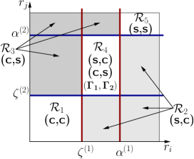
Figure 2: Illustration of the various regions along with the NE strategies corresponding to these regions.

--------------------------------------------------------------------------------------

$$\mathcal{T}_{1}(\mathbf{C}) = \tau+\sum_{(i,j)\in\mathcal{R}_{1}(\mathbf{C})}p_{i,j}C^{(1)}+\sum_{(i,j)\in\mathcal{R}_{2}(\mathbf{C})\cup\mathcal{R}_{4}(\mathbf{C})}p_{i,j}(-\eta_{1}r_{i})+\sum_{(i,j)\in\mathcal{R}_{3}(\mathbf{C})}p_{i,j}D^{(1)}+\sum_{(i,j)\in\mathcal{R}_{5}(\mathbf{C})}p_{i,j}E^{(1)}(r_{i})$$ (36)

$$\mathcal{T}_{2}(\mathbf{C}) = \tau+\sum_{(i,j)\in\mathcal{R}_{1}(\mathbf{C})}p_{i,j}C^{(2)}+\sum_{(i,j)\in\mathcal{R}_{2}(\mathbf{C})\cup\mathcal{R}_{4}(\mathbf{C})}p_{i,j}D^{(2)}+\sum_{(i,j)\in\mathcal{R}_{3}(\mathbf{C})}p_{i,j}(-\eta_{2}r_{j})+\sum_{(i,j)\in\mathcal{R}_{5}(\mathbf{C})}p_{i,j}E^{(2)}(r_{j}).$$ (37)

Discussion: The above lemma becomes intuitive once we recall that $D^{(1)}$ is the optimal cost incurred by $\mathscr{F}_{1}$ if it is alone in the system, while $C^{(1)}_{\pi_{1}^{*},\pi_{2}^{*}}$ is the cost incurred if $\mathscr{F}_{2}$ is also present, and competing with $\mathscr{F}_{1}$ in choosing a relay. One would expect $\mathscr{F}_{1}$ to incur a lower cost without the competing forwarder.

For notational simplicity, from here on, we will denote the costs $C^{(1)}_{\pi_{1}^{*},\pi_{2}^{*}}$ and $C^{(2)}_{\pi_{1}^{*},\pi_{2}^{*}}$ as simply $C^{(1)}$ and $C^{(2)}$. We will write $\mathbf{C}$ for the pair $(C^{(1)},C^{(2)})$. An important consequence of Lemma 2 is that, while solving the game in Table 4, it is sufficient to only consider cost pairs, $(C^{(1)},C^{(2)})$, which are ordered as in the lemma; the other cases (e.g., $D^{(1)}>C^{(1)}$ or $D^{(2)}>C^{(2)}$) cannot occur, and hence need not be considered. Further, for convenience let us denote the thresholds $\frac{C^{(1)}}{-\eta_{1}}$ and $\frac{C^{(2)}}{-\eta_{2}}$ by $\zeta^{(1)}$ and $\zeta^{(2)}$, respectively (recall that we already have, $\alpha^{(1)}=\frac{D^{(1)}}{-\eta_{1}}$ and $\alpha^{(2)}=\frac{D^{(2)}}{-\eta_{2}}$). Then, the solution (i.e., the NE strategies) to the game in Table 4, for each $(r_{i},r_{j})$ pair, is as depicted in Fig. 2.

We see that the thresholds $(\alpha^{(1)},\zeta^{(1)})$ and $(\alpha^{(2)},\zeta^{(2)})$ partition the reward pair set, $\{(r_{i},r_{j}):i,j\in[n]\}$, into $5$ regions ($\mathcal{R}_{1},\cdots,\mathcal{R}_{5}$) such that the NE strategy (strategies) corresponding to each region are different. For instance, for any $(r_{i},r_{j})\in\mathcal{R}_{1}$, $(\textsf{c},\textsf{c})$ (i.e., both forwarders continue) is the only NE strategy, while within $\mathcal{R}_{2}$, $(\textsf{s},\textsf{c})$ is the NE strategy, and so on. All regions contain a unique pure NE strategy except for $\mathcal{R}_{4}$ where $(\textsf{s},\textsf{c})$, $(\textsf{c},\textsf{s})$, and the mixed strategy $(\Gamma_{1},\Gamma_{2})$ ($\Gamma_{\rho}$ is the probability with which $\mathscr{F}_{\rho}$ chooses s) are all NE strategies. The expression for $\Gamma_{1}$ is

$$\Gamma_{1}=\frac{-\eta_{2}r_{j}-C^{(2)}}{\Big{(}-\eta_{2}r_{j}-C^{(2)}\Big{)}-\Big{(}E^{(2)}(r_{j})-D^{(2)}\Big{)}}.$$ (38)

Analogously one can write the expression for $\Gamma_{2}$. For details on how to solve the game in Table 4 to obtain the various regions, see Appendix D. Finally, we summarize the observations made thus far in the form of the following theorem.

Theorem 2

The NE strategies of the game in Table 4 are completely characterized by the threshold pairs $(\alpha^{(\rho)},\zeta^{(\rho)})$, $\rho=1,2$ as follows (recall Fig. 2 for illustration):

• If $r_{i}$ is less than $\zeta^{(1)}$, then the NE strategy recommends c for $\mathscr{F}_{1}$ irrespective of the reward value $r_{j}$ of $\mathscr{F}_{2}$.

• On the other hand, if $r_{i}$ is more than $\alpha^{(1)}$, then the NE strategy recommends action s for $\mathscr{F}_{1}$ irrespective of the value of $r_{j}$ (note that this is exactly the action $\mathscr{F}_{1}$ would choose if it was alone in the system; see the discussion following (25)).

• Finally, the presence of the competing forwarder $\mathscr{F}_{2}$ is felt by $\mathscr{F}_{1}$ only when its reward value $r_{i}$ is between $\zeta^{(1)}$ and $\alpha^{(1)}$, in which case the NE strategies are: $(\textsf{s},\textsf{c})$ if $r_{j}<\zeta^{(2)}$; $(\textsf{s},\textsf{c})$, $(\textsf{c},\textsf{s})$ and $(\Gamma_{1},\Gamma_{2})$ if $\zeta^{(2)}\leq r_{j}\leq\alpha^{(2)}$; and $(\textsf{c},\textsf{s})$ if $r_{j}>\alpha^{(2)}$.

Analogous results hold for $\mathscr{F}_{2}$.

V-C Constructing NEPPs from NE strategies

The cost terms $D^{(1)}$ and $D^{(2)}$ can be easily computed by solving the optimality equations (21) and (27), respectively. Alternatively, we can first compute the fixed points of $\beta^{(1)}(\cdot)$ and $\beta^{(2)}(\cdot)$ to obtain $\alpha^{(1)}$ and $\alpha^{(2)}$, respectively (recall Lemma 1). Then, $D^{(1)}=-\eta_{1}\alpha^{(1)}$ and $D^{(2)}=-\eta_{2}\alpha^{(2)}$.

The costs $C^{(1)}$ and $C^{(2)}$ (in (33) and (34)) depend on the particular NEPP used, i.e., require the cost terms $J^{(1)}_{\pi_{1}^{*},\pi_{2}^{*}}(r_{i},r_{j})$ and $J^{(2)}_{\pi_{1}^{*},\pi_{2}^{*}}(r_{i},r_{j})$ for all $(r_{i},r_{j})$ to compute them. Conversely, Part-(b) of Theorem 1 suggests that $J^{(1)}_{\pi_{1}^{*},\pi_{2}^{*}}(r_{i},r_{j})$ (respectively, $J^{(2)}_{\pi_{1}^{*},\pi_{2}^{*}}(r_{i},r_{j})$) can be obtained by computing the expected cost incurred by $\mathscr{F}_{1}$ (respectively, $\mathscr{F}_{2}$) at a NE strategy of the game in Table 4, which in turn requires the terms $C^{(1)}$ and $C^{(2)}$. Hence, to obtain $(C^{(1)},C^{(2)})$ we proceed by expressing $(C^{(1)},C^{(2)})$ as the fixed point of a mapping $\mathcal{T}$ which can then be used to compute these costs.

Suppose $(\pi_{1}^{*},\pi_{2}^{*})$ is a NEPP such that for all $x=(r_{i},r_{j})\in\mathcal{R}_{4}(\mathbf{C})$ the NE strategy $(\pi_{1}^{*}(x),\pi_{2}^{*}(x))$ is $(\textsf{s},\textsf{c})$. Then using part 2(b) of Theorem 1 we can write,

$$J^{(1)}_{\pi_{1}^{*},\pi_{2}^{*}}(r_{i},r_{j})=\left\{\begin{array}[]{cl}C^{(1)}&\mbox{ if }(r_{i},r_{j})\in\mathcal{R}_{1}(\mathbf{C})\\ -\eta_{1}r_{i}&\mbox{ if }(r_{i},r_{j})\in\mathcal{R}_{2}(\mathbf{C})\\ D^{(1)}&\mbox{ if }(r_{i},r_{j})\in\mathcal{R}_{3}(\mathbf{C})\\ -\eta_{1}r_{i}&\mbox{ if }(r_{i},r_{j})\in\mathcal{R}_{5}(\mathbf{C})\\ E^{(1)}(r_{i})&\mbox{ if }(r_{i},r_{j})\in\mathcal{R}_{4}(\mathbf{C}).\end{array}\right.$$ (44)

Using the above in (33), $C^{(1)}$ can be written as $C^{(1)}=\mathcal{T}_{1}(\mathbf{C})$ where the function $\mathcal{T}_{1}(\mathbf{C})$ is as in (36) (where for simplicity, we have used $(i,j)$ instead of $(r_{i},r_{j})$). Similarly, $C^{(2)}$ can be expressed as $C^{(2)}=\mathcal{T}_{2}(\mathbf{C})$; see (37). Thus, $\mathbf{C}$ is a fixed point of the mapping $\mathcal{T}(\mathbf{C}):=(\mathcal{T}_{1}(\mathbf{C}),\mathcal{T}_{2}(\mathbf{C}))$.

We do not have results showing that $\mathcal{T}$ indeed has a fixed point or equivalently that an NEPP $(\pi_{1}^{*},\pi_{2}^{*})$ always exists, although such a result holds for the discounted stochastic game [29, Theorem 4.6.4] (recall that ours is a transient stochastic game). However, in our numerical results section (Section VIII) we were able to numerically obtain $\mathbf{C}$ by iteration. Thus, we begin with an initial $\mathbf{C}(0)$ such that $C^{(1)}(0)<D^{(1)}$ and $C^{(2)}(0)<D^{(2)}$, and inductively iterate to obtain $\mathbf{C}(k)=\mathcal{T}(\mathbf{C}(k-1))$ until convergence is achieved. Finally, given a fixed point $\mathbf{C}$, we obtain the corresponding NEPP $(\pi_{1}^{*},\pi_{2}^{*})$ by constructing the various regions as in Fig. 2.

Other NEPPs: Recall that to obtain $(C^{(1)},C^{(2)})$ we had restricted $(\pi_{1}^{*},\pi_{2}^{*})$ to use NE strategy $(\textsf{s},\textsf{c})$ whenever $(r_{i},r_{j})\in\mathcal{R}_{4}(\mathbf{C})$. We can similarly obtain NEPPs $({\pi_{1}^{\circ}},{\pi_{2}^{\circ}})$ and $({\pi_{1}^{\Box}},{\pi_{2}^{\Box}})$ (whose corresponding cost pairs are $\mathbf{C}_{\circ}$ and $\mathbf{C}_{\Box}$) by restricting to the NE strategies $(\textsf{c},\textsf{s})$ and $(\Gamma_{1},\Gamma_{2})$ whenever $(r_{i},r_{j})\in\mathcal{R}_{4}(\mathbf{C}_{\circ})$ and $(r_{i},r_{j})\in\mathcal{R}_{4}(\mathbf{C}_{\Box})$, respectively. In Section VIII we will numerically compare the performances of all these various NEPPs.

VI Partially Observable Case

Let us first formally introduce a finite location set $\mathcal{L}$. Let $L_{k}$ denote the location of the $k$-th relay. The locations $\{L_{k}:k\geq 1\}$ are i.i.d with their common p.m.f. being $(q_{\ell}:\ell\in\mathcal{L})$. Recall that for the PO case we assume that only $R_{\rho,k}$ is revealed to $\mathscr{F}_{\rho}$ ($\rho=1,2$). In addition, we will assume that $L_{k}$ is revealed to both the forwarders.

Recalling the geographical forwarding example from Section III, the PO case corresponds to the scenario where, in addition to $L_{k}$, the gains $G_{\rho,k}$ are required to compute $R_{\rho,k}$, i.e., if $a<1$ in (8). Hence, $\mathscr{F}_{1}$ not knowing $G_{2,k}$ cannot compute $R_{2,k}$. However, knowing the channel gain distribution (recall that the gains are identically distributed) it is possible for $\mathscr{F}_{1}$ to compute the probability distribution of $R_{2,k}$ given $L_{k}$. Similarly, $\mathscr{F}_{2}$ can compute the distribution of $R_{1,k}$ given $L_{k}$. Further, since the gains, $(G_{1,k},G_{2,k})$, are independent, it follows that $R_{1,k}$ and $R_{2,k}$ are independent given $L_{k}$ (but unconditionally they may be dependent).

Formally, given that $L_{k}=\ell$, we will assume the following independence condition:

$$p_{R_{1},R_{2}|L_{k}}(r_{i},r_{j}|\ell)=p_{R_{1}|L_{k}}(r_{i}|\ell)p_{R_{2}|L_{k}}(r_{j}|\ell).$$ (45)

For simplicity, we will denote the conditional p.m.f.s $p_{R_{1}|L_{k}}(r_{i}|\ell)$ and $p_{R_{2}|L_{k}}(r_{j}|\ell)$, $i,j\in[n]$, by $p^{(1)}_{i|\ell}$ and $p^{(2)}_{j|\ell}$, respectively.

Remark: Usually for a model with partial observations the belief that $\mathscr{F}_{1}$ will maintain about $R_{2,k}$ will simply be the conditional distribution $p_{R_{2}|R_{1}}(r_{j}|r_{i})$ $=\frac{p_{i,j}}{p^{(1)}_{i}}$. However, we have exploited the particular structure in our reward expression to come up with the independence condition in (45). This condition will enable us to prove a key result later which is otherwise not possible (see the remark following Lemma 4). Finally, all our subsequent results will hold for a more general model wherever the independence condition in (45) will hold.

We will now proceed to formulate our partially observable model as a partially observable stochastic game (POSG). We will first formally describe the problem setting and then briefly discuss POSGs, before proceeding to our main results.

VI-A Problem Formulation

The actual state space of the system continues to be $\mathcal{X}$ (see (1)). However, each forwarder now gets to observe only its part of the actual state (i.e., only its reward value) along with the relay’s location. Thus, when the $k$-th relay arrives, and if both forwarders are still competing then the observations of $\mathscr{F}_{1}$ and $\mathscr{F}_{2}$ are of the form $(r_{i},\ell)$ and $(\ell,r_{j})$, respectively, where $(r_{i},r_{j})$ is the actual state, $L_{k}=\ell$ is the location of the $k$-th relay. Suppose $\mathscr{F}_{2}$ has already terminated before stage $k$ then the location information is no more required by $\mathscr{F}_{1}$, and hence we will denote its observation as $(r_{i},\textbf{\emph{t}})$ which is simply the system state. Finally, when $\mathscr{F}_{1}$ terminates we use t to denote its subsequent observations. Thus, we can write the observation space of $\mathscr{F}_{1}$ as,

$$\mathcal{O}_{1} = \Big{\{}(r_{i},\ell),(r_{i},\textbf{\emph{t}}),\textbf{\emph{t}}:i\in[n],\ell\in[m]\Big{\}}.$$ (46)

Similarly, the observation space of $\mathscr{F}_{2}$ is given by

$$\mathcal{O}_{2} = \Big{\{}(\ell,r_{j}),(\textbf{\emph{t}},r_{j}),\textbf{\emph{t}}:j\in[n],\ell\in[m]\Big{\}}.$$ (47)

Definition 3

We will modify the definition of a policy pair, $(\overline{\pi}_{1},\overline{\pi}_{2})$ (see Definition 1), such that $\overline{\pi}_{1}:\mathcal{O}_{1}\rightarrow\{\textsf{s},\textsf{c}\}$ and $\overline{\pi}_{2}:\mathcal{O}_{2}\rightarrow\{\textsf{s},\textsf{c}\}$. Thus, the decision to stop or continue by $\mathscr{F}_{1}$ and $\mathscr{F}_{2}$, when the $k$-th relay arrives is based on their respective observations $o_{1,k}\in\mathcal{O}_{1}$ and $o_{2,k}\in\mathcal{O}_{2}$.

Remark: Note that we have restricted the PO policies to be deterministic (and as before stationary), i.e., $\overline{\pi}_{1}(o_{1})$ is either s or c without mixing between the two. Let $\Pi_{D}$ denote the set of all such deterministic policies. Restricting to $\Pi_{D}$ is primarily to simplify the analysis. However, it is not immediately clear if a partially observable NEPP (to be formally defined very soon) should even exist within the class $\Pi_{D}$. Our main result is to construct a Bayesian stage game and prove that this game contains pure strategy (or deterministic) NE vectors using which PO-NEPPs in $\Pi_{D}$ can be constructed.

Let $\{(O_{1,k},O_{2,k})$: $k\geq 1\}$, denote the sequence of joint-observation at stage $k$, and let $\{X_{k}:k\geq 1\}$ as before denote the sequence of states. Then the expected cost incurred by $\mathscr{F}_{\rho}$, $\rho=1,2$, when the PO policy pair used is $(\overline{\pi}_{1},\overline{\pi}_{2})$, and when its initial observation is $o_{\rho}$, can be written as

$$G^{(\rho)}_{\overline{\pi}_{1},\overline{\pi}_{2}}(o_{\rho})=\sum_{k=1}^{\infty}\mathbb{E}^{o_{\rho}}_{\overline{\pi}_{1},\overline{\pi}_{2}}\bigg{[}g_{\rho}(X_{k},(A_{1,k},A_{2,k}))\bigg{]},$$ (48)

where $A_{1,k}=\overline{\pi}_{1}(O_{1,k})$ and $A_{2,k}=\overline{\pi}_{2}(O_{2,k})$.

Similar to the completely observable case, the objective for the partially observable (PO) case is to characterize PO-NEPPs which are defined as follows:

Definition 4

We say that a PO policy pair $(\overline{\pi}_{1}^{*},\overline{\pi}_{2}^{*})$ is a PO-NEPP if $G^{(1)}_{\overline{\pi}_{1}^{*},\overline{\pi}_{2}^{*}}(o_{1})\leq G^{(1)}_{\overline{\pi}_{1},\overline{\pi}_{2}^{*}}(o_{1})$ for all $o_{1}\in\mathcal{O}_{1}$ and PO policy $\overline{\pi}_{1}\in\Pi_{D}$, and $G^{(2)}_{\overline{\pi}_{1}^{*},\overline{\pi}_{2}^{*}}(o_{2})\leq G^{(2)}_{\overline{\pi}_{1}^{*},\overline{\pi}_{2}}(o_{2})$ where $o_{2}\in\mathcal{O}_{2}$ and $\overline{\pi}_{2}\in\Pi_{D}$.

We will end this section with the expressions for the various cost terms corresponding to a PO-NEPP, which are analogues of the cost terms in Section V.

Various Cost Terms: Recall the expression for $D^{(1)}$ from (22). Given a NEPP $(\pi_{1}^{*},\pi_{2}^{*})$, $D^{(1)}$ is the cost incurred by $\mathscr{F}_{1}$ if it continues alone. Similar expressions can be written for a PO-NEPP $(\overline{\pi}_{1}^{*},\overline{\pi}_{2}^{*})$:

$$\overline{D}^{(1)} = \tau+\sum_{i^{\prime}}p^{(1)}_{i^{\prime}}{G}^{(1)}_{\overline{\pi}_{1}^{*},\overline{\pi}_{2}^{*}}(r_{i^{\prime}},\textbf{\emph{t}}).$$ (49)

Similarly, for $\mathscr{F}_{2}$, the cost of continuing alone is

$$\overline{D}^{(2)} = \tau+\sum_{j^{\prime}}p^{(2)}_{j^{\prime}}{G}^{(2)}_{\overline{\pi}_{1}^{*},\overline{\pi}_{2}^{*}}(\textbf{\emph{t}},r_{j^{\prime}}).$$ (50)

The following lemma will be useful.

Lemma 3

Let $(\pi_{1}^{*},\pi_{2}^{*})$ be an NEPP and $(\overline{\pi}_{1}^{*},\overline{\pi}_{2}^{*})$ be a PO-NEPP then $J^{(1)}_{\pi_{1}^{*},\pi_{2}^{*}}(r_{i},\textbf{\emph{t}})=G^{(1)}_{\overline{\pi}_{1}^{*},\overline{\pi}_{2}^{*}}(r_{i},\textbf{\emph{t}})$ and $J^{(2)}_{\pi_{1}^{*},\pi_{2}^{*}}(\textbf{\emph{t}},r_{j})=G^{(2)}_{\overline{\pi}_{1}^{*},\overline{\pi}_{2}^{*}}(\textbf{\emph{t}},r_{j})$.

Proof:

Whenever $\mathscr{F}_{1}$ is alone in the system, all its observations (which are of the form $(r_{i},\textbf{\emph{t}})$ until $\mathscr{F}_{1}$ terminates) are exactly the actual states traversed by the system. Hence the problem of obtaining $G^{(1)}_{\overline{\pi}_{1}^{*},\overline{\pi}_{2}^{*}}(r_{i},\textbf{\emph{t}})$ is identical to the MDP problem of obtaining $J^{(1)}_{\pi_{1}^{*},\pi_{2}^{*}}(r_{i},\textbf{\emph{t}})$ in Section V-B, so that $G^{(1)}_{\overline{\pi}_{1}^{*},\overline{\pi}_{2}^{*}}(r_{i},\textbf{\emph{t}})$ satisfies the Bellman equation in (21). Since the solution to (21) is unique [39] we obtain $J^{(1)}_{\pi_{1}^{*},\pi_{2}^{*}}(r_{i},\textbf{\emph{t}})=G^{(1)}_{\overline{\pi}_{1}^{*},\overline{\pi}_{2}^{*}}(r_{i},\textbf{\emph{t}})$. Similarly it follows that $J^{(2)}_{\pi_{1}^{*},\pi_{2}^{*}}(\textbf{\emph{t}},r_{j})=G^{(2)}_{\overline{\pi}_{1}^{*},\overline{\pi}_{2}^{*}}(\textbf{\emph{t}},r_{j})$. ∎

Discussion: An immediate consequence of the above lemma is that $\overline{D}^{(1)}=D^{(1)}$ and $\overline{D}^{(2)}=D^{(2)}$. Further, if $(\overline{\pi}_{1}^{*},\overline{\pi}_{2}^{*})$ is a PO-NEPP then for states of the form $(r_{i},\textbf{\emph{t}})$, $\overline{\pi}_{1}^{*}(r_{i},\textbf{\emph{t}})$ is same as $\pi_{1}^{*}(r_{i},\textbf{\emph{t}})$ in (25). Similarly, for states of the form $(\textbf{\emph{t}},r_{j})$, $\overline{\pi}_{2}^{*}(\textbf{\emph{t}},r_{j})$ is same as that in (30).

However, the analogues of the cost terms $C^{(1)}_{\pi_{1},\pi_{2}}$ and $C^{(2)}_{\pi_{1},\pi_{2}}$ (recall (33) and (34)) are different for the partially observable case. The expressions for these are,

$$\overline{C}^{(1)}_{\overline{\pi}_{1},\overline{\pi}_{2}} = \tau+\sum_{\ell^{\prime},i^{\prime}}q_{\ell^{\prime}}\cdot p^{(1)}_{i^{\prime}|\ell^{\prime}}\cdot G^{(1)}_{\overline{\pi}_{1},\overline{\pi}_{2}}(r_{i^{\prime}},\ell^{\prime}),$$ (51)

$$\overline{C}^{(2)}_{\overline{\pi}_{1},\overline{\pi}_{2}} = \tau+\sum_{\ell^{\prime},j^{\prime}}q_{\ell^{\prime}}\cdot p^{(2)}_{j^{\prime}|\ell^{\prime}}\cdot G^{(2)}_{\overline{\pi}_{1},\overline{\pi}_{2}}(\ell^{\prime},r_{j^{\prime}}).$$ (52)

Finally, similar to the result in Lemma 2, we can show that for a PO-NEPP $(\overline{\pi}_{1}^{*},\overline{\pi}_{2}^{*})$,

$$\overline{D}^{(1)}\leq\overline{C}^{(1)}_{\overline{\pi}_{1}^{*},\overline{\pi}_{2}^{*}}\mbox{ and }\overline{D}^{(2)}\leq\overline{C}^{(2)}_{\overline{\pi}_{1}^{*},\overline{\pi}_{2}^{*}}.$$ (53)

The proof of these is along exactly the same lines as the proof of Lemma 2. We do not repeat it for brevity.

VI-B Partially Observable Stochastic Game (POSG)

A POSG is a tuple $(\mathcal{N},\mathcal{X},\mathcal{O},\{\mathcal{A}_{\rho}\},\hat{T},\{{g}_{\rho}\})$, where $\mathcal{N}$, $\mathcal{X}$, $\mathcal{A}_{\rho}$, and ${g}_{\rho}$ are as before (see Section V-A), while

• $\mathcal{O}=\times_{\rho\in\mathcal{N}}\mathcal{O}_{\rho}$ is the joint-observation space, with $\mathcal{O}_{\rho}$ being the observation space of player $\rho$, and

• $\hat{T}:\mathcal{X}\times\mathcal{O}\times\mathcal{A}\rightarrow\Delta(\mathcal{X}\times\mathcal{O})$ is the transition function where $\hat{T}(x^{\prime},o^{\prime}|x,o,a)$ is the probability that the next state and the joint-observation is $(x^{\prime},o^{\prime})$ conditioned on the event that the current state, joint-observation and joint-action is $(x,o,a)$.

In the previous section we have seen that the NEPPs for a stochastic game can be obtained by constructing a normal-form static stage game. Similarly for POSGs, there is work (for instance see, [40]) that constructs a game which is effectively played at each stage, however, with the players not knowing the exact state of the system the stage game now happens to be a Bayesian game [41, Chapter 9]. Hence, the drawback with POSGs in general is that, at each stage $k$, each player needs to maintain a belief (distribution) about the entire history of joint-observations and joint-actions,

$((o_{1,1},o_{2,1}),(a_{1,1},a_{1,2}),\cdots,(a_{1,k-1},a_{2,k-1}),(o_{1,k},o_{2,k})$,

(referred to as the joint-type of the Bayesian game), obtaining which for a general POSG is computationally intensive.

For this reason the authors in [42] have studied a restriction of POSGs referred to as, Markov games of Incomplete information (MGII). In MGIIs the transition function $\hat{T}$ satisfies the following Markov property: player-1’s belief about the player-2’s current observation, $o^{\prime}_{2}$, is independent of player-2’s previous observation, $o_{2}$, given the current state, $x^{\prime}$, previous state, $x$, and player-1’s current and previous observations, ${o^{\prime}}_{1}$ and $o_{1}$, respectively, i.e., for two different observations $u,v\in\mathcal{O}_{2}$ of player-2, $\hat{T}({o^{\prime}}_{2}|x^{\prime},x,{o^{\prime}}_{2},o_{1},o_{2}=u)=\hat{T}({o^{\prime}}_{2}|x^{\prime},x,{o^{\prime}}_{1},o_{1},o_{2}=v)$. Similar Markov structure should hold for other players also. For our case it is easy to check that the above condition is trivially satisfied, primarily because all the associated random variables, $\{L_{k}\}$ and $\{(R_{1,k},R_{2,k})\}$, are i.i.d. across the stage index $k$.

A major advantage with MGIIs is that the current joint-observation constitutes the type of the Bayesian game to be played at that stage. With this in mind, we will set up a Bayesian stage game in the next section, with $(r_{i},\ell)$ and $(\ell,r_{j})$ constituting the type of the game at stage $k$, provided both forwarders are still competing at stage $k$.

VI-C Bayesian Stage Game

We are now ready to provide a solution to the partially observable case in terms of a certain Bayesian game [41, Chapter 9] which is effectively played at any stage whenever both forwarders are contending. For the completely observable case, given a policy pair $(\pi_{1},\pi_{2})$, corresponding to each $(r_{i},r_{j})$ pair we constructed the normal-form game in Table 4. However here, given a PO policy pair $(\pi_{1},\pi_{2})$ and given the observation $(r_{i},\ell)$, $\mathscr{F}_{1}$’s belief that the game in Table 4 (with $(C^{(1)}_{\pi_{1},\pi_{2}},C^{(2)}_{\pi_{1},\pi_{2}})$ replaced by $(\overline{C}^{(1)}_{\overline{\pi}_{1},\overline{\pi}_{2}}\overline{C}^{(2)}_{\overline{\pi}_{1},\overline{\pi}_{2}})$) will be played is $p^{(2)}_{j|\ell}$, $j\in[n]$. Hence, $\mathscr{F}_{1}$ needs to first compute the costs incurred for playing s and c, averaged over all observations $(\ell,r_{j})$, $j\in[n]$, of $\mathscr{F}_{2}$. We will formally develop these in the following.

Strategy vectors and corresponding costs: Fixing the PO-policy pair to be $(\overline{\pi}_{1},\overline{\pi}_{2})$ (unless otherwise stated), we will refer to the subsequent development (which includes, the strategy vectors, various costs, best responses and NE vectors, to be discussed next) as the Bayesian game corresponding to $(\overline{\pi}_{1},\overline{\pi}_{2})$, denoted $\mathcal{G}(\overline{\pi}_{1},\overline{\pi}_{2})$.

Definition 5

For $\ell\in\mathcal{L}$ (recall that $\mathcal{L}$ is the set of possible relay locations), we define a strategy vector, $f_{\ell}$, of $\mathscr{F}_{1}$ as $f_{\ell}:\{r_{i}:i\in[n]\}\rightarrow\{\textsf{s},\textsf{c}\}$. Similarly, a strategy vector $g_{\ell}$ of $\mathscr{F}_{2}$ is $g_{\ell}:\{r_{j}:j\in[n]\}\rightarrow\{\textsf{s},\textsf{c}\}$. Thus, given the observation $(r_{i},\ell)$ of $\mathscr{F}_{1}$, $f_{\ell}$ decides for $\mathscr{F}_{1}$ whether to stop or continue.

Now, given the strategy vector $g_{\ell}$ of $\mathscr{F}_{2}$, and the location information $\ell$, $\mathscr{F}_{1}$’s belief that $\mathscr{F}_{2}$ will choose action c is

$$\widetilde{g}_{\ell} = \sum_{j:g_{\ell}(r_{j})=\textsf{c}}p^{(2)}_{j|\ell};$$ (54)

$(1-\widetilde{g}_{\ell})$ is the probability that $\mathscr{F}_{2}$ will stop. Thus, the expected cost incurred by $\mathscr{F}_{1}$ for playing s when its observation is $(r_{i},\ell)$ and when $\mathscr{F}_{2}$ uses ${g}_{\ell}$ is

$$C_{\textsf{s},g_{\ell}}^{(1)}(r_{i}) = \widetilde{g}_{\ell}(-\eta_{1}r_{i})+(1-\widetilde{g}_{\ell})E^{(1)}(r_{i}),$$ (55)

where, recall from (31) that $E^{(1)}(r_{i})=\nu_{1}(-\eta_{1}r_{i})+\nu_{2}{D}^{(1)}$. The various terms in (55) can be understood as follows: $\widetilde{g}_{\ell}$ is the probability that $\mathscr{F}_{2}$ will continue in which case $\mathscr{F}_{1}$ (having chosen the action s) stops, incurring a terminating cost of $-\eta_{1}r_{i}$, while $(1-\widetilde{g}_{\ell})$ is the probability that $\mathscr{F}_{2}$ will stop in which case the expected cost is, $\nu_{1}(-\eta_{1}r_{i})+\nu_{2}{D}^{(1)}$; $\nu_{1}$ is the probability that $\mathscr{F}_{1}$ gets the relay and terminates incurring a cost of $(-\eta_{1}r_{i})$, otherwise w.p. $\nu_{2}$, $\mathscr{F}_{2}$ gets the relay in which case $\mathscr{F}_{1}$ continues alone, the expected cost of which is $\overline{D}^{(1)}=D^{(1)}$ (from Lemma 3).

The expected cost of continuing when $\mathscr{F}_{1}$’s observation is $(r_{i},\ell)$ is

$$C_{\textsf{c},{g}_{\ell}}^{(1)}(r_{i}) = \widetilde{g}_{\ell}\overline{C}^{(1)}_{\overline{\pi}_{1},\overline{\pi}_{2}}+(1-\widetilde{g}_{\ell})D^{(1)}.$$ (56)

From the above expression we see that the cost of continuing is a constant in the sense that it does not depend on the value of $r_{i}$. Hence we will denote it as simply $C_{\textsf{c},g_{\ell}}^{(1)}$. Further, note that $C_{\textsf{c},g_{\ell}}^{(1)}$ depends on the PO policy pair $(\overline{\pi}_{1},\overline{\pi}_{2})$, but for simplicity we have not shown this dependence in the notation for $C_{\textsf{c},g_{\ell}}^{(1)}$.

Similarly for $\mathscr{F}_{2}$, when its observation is $(\ell,r_{j})$ and when $\mathscr{F}_{1}$ uses ${f}_{\ell}$, we have

$$C^{(2)}_{\textsf{s},{f}_{\ell}}(r_{j}) = \widetilde{f}_{\ell}(-\eta_{2}r_{j})+(1-\widetilde{f}_{\ell})E^{(2)}(r_{j})$$

$$C_{\textsf{c},{f}_{\ell}}^{(2)} = \widetilde{f}_{\ell}\overline{c}^{(2)}_{\overline{\pi}_{1}^{*},\overline{\pi}_{2}^{*}}+(1-\widetilde{f}_{\ell})D^{(2)},$$

where $\widetilde{f}_{\ell}=\underset{i:{f}_{\ell}(r_{i})=\textsf{c}}{\sum}p^{(1)}_{i|\ell}$.

Definition 6

We say that ${f}_{\ell}$ is the best response vector of $\mathscr{F}_{1}$ against the strategy vector ${g}_{\ell}$ played by $\mathscr{F}_{2}$, denoted ${f}_{\ell}=BR_{1}({g}_{\ell})$, if ${f}_{\ell}(r_{i})=\textsf{s}$ iff $C^{(1)}_{\textsf{s},{g}_{\ell}}(r_{i})\leq C^{(1)}_{\textsf{c},{g}_{\ell}}$. Note that such an ${f}_{\ell}$ is unique. Similarly, ${g}_{\ell}$ is the (unique) best response against ${f}_{\ell}$ if, ${g}_{\ell}(r_{j})=\textsf{s}$ iff $C^{(2)}_{\textsf{s},{f}_{\ell}}(r_{j})\leq C^{(2)}_{\textsf{c},{f}_{\ell}}$. We denote this as ${g}_{\ell}=BR_{2}({f}_{\ell})$.

Definition 7

For $\ell\in\mathcal{L}$, a pair of strategy vectors $({f}_{\ell}^{*},{g}_{\ell}^{*})$ is said to be a Nash equilibrium (NE) vector for the game $\mathcal{G}(\overline{\pi}_{1},\overline{\pi}_{2})$ iff ${f}_{\ell}^{*}=BR_{1}({g}_{\ell}^{*})$, and ${g}_{\ell}^{*}=BR_{2}({f}_{\ell}^{*})$.

As remarked earlier, it is not immediately clear whether a NE vector should even exist among the pure strategies for the game $\mathcal{G}(\overline{\pi}_{1},\overline{\pi}_{2})$. Our main result in the next section (Theorem 4) is to provide a positive answer to this. In fact, we will not only prove the existence of NE vectors but also provide a method to construct them.

We will end this section with the following theorem which is similar to Theorem 1-(b), that was used to obtain NEPPs. This theorem will enable us to construct PO-NEPPs.

Theorem 3

Given a PO policy pair $(\overline{\pi}_{1}^{*},\overline{\pi}_{2}^{*})$, construct the strategy vector pair $\{({f}_{\ell}^{*},{g}_{\ell}^{*}):\ell\in\mathcal{L}\}$ as follows: $f_{\ell}^{*}(r_{i})=\overline{\pi}_{1}^{*}(r_{i},\ell)$ and ${g}_{\ell}^{*}(r_{j})=\overline{\pi}_{2}^{*}(\ell,r_{j})$ for all $i,j\in[n]$. Now, suppose for each $\ell$, $({f}_{\ell}^{*},{g}_{\ell}^{*})$ is a NE vector for the game $\mathcal{G}(\overline{\pi}_{1}^{*},\overline{\pi}_{2}^{*})$ such that,

$$\min\Big{\{}C^{(1)}_{\textsf{s},{g}_{\ell}^{*}}(r_{i}),C^{(1)}_{\textsf{c},{g}_{\ell}^{*}}\Big{\}} = G^{(1)}_{\overline{\pi}_{1}^{*},\overline{\pi}_{2}^{*}}(r_{i},\ell),\mbox{ and }$$ (57)

$$\min\Big{\{}C^{(2)}_{\textsf{s},f_{\ell}^{*}}(r_{j}),C^{(2)}_{\textsf{c},f_{\ell}^{*}}\Big{\}} = G^{(2)}_{\overline{\pi}_{1}^{*},\overline{\pi}_{2}^{*}}(\ell,r_{j}).$$ (58)

Then $(\overline{\pi}_{1}^{*},\overline{\pi}_{2}^{*})$ is a PO-NEPP.

Proof:

See Appendix E. ∎

Discussion: If $\{({f}_{\ell}^{*},{g}_{\ell}^{*})\}$ happens to be a NE vector, then from Definition 7 it simply follows that the LHS of (57) (resp. (58)) is simply the cost incurred by $\mathscr{F}_{1}$ (resp. $\mathscr{F}_{2}$) for playing the action, $f_{\ell}^{*}(r_{i})$ (resp. ${g}_{\ell}^{*}(r_{j})$), suggested by its NE vector. Thus, (57) and (58) collective say that the cost-pair obtained by playing the NE vector $({f}_{\ell}^{*},{g}_{\ell}^{*})$ in the Bayesian game $\mathcal{G}(\overline{\pi}_{1}^{*},\overline{\pi}_{2}^{*})$, is equal to the cost-pair incurred by the PO policy pair $(\overline{\pi}_{1}^{*},\overline{\pi}_{2}^{*})$ in the original POSG. Hence, this result could be thought of as the analogue of Theorem 1-(b) proved for the completely observable case.

Existence of a NE Vector: We will fix a PO policy pair $(\overline{\pi}_{1}^{*},\overline{\pi}_{2}^{*})$ that satisfies the inequalities in (53). In this section we will prove that there exists a NE vector for $\mathcal{G}(\overline{\pi}_{1}^{*},\overline{\pi}_{2}^{*})$. Before proceeding to the main theorem we need the following results (Lemma 4 and 5).

Lemma 4

For any $\ell\in\mathcal{L}$, the best response vector, $f_{\ell}$, against any vector $g_{\ell}$ of $\mathscr{F}_{2}$ is a threshold vector, i.e., there exists an $\Phi_{\ell}\in\{0,1,\cdots,n\}$ such that $f_{\ell}(r_{i})=\textsf{s}$ iff $i>\Phi_{\ell}$. We refer to $\Phi_{\ell}$ as the threshold of $f_{\ell}$. Similarly, if $g_{\ell}$ is the best response against any vector $f_{\ell}$ of $\mathscr{F}_{1}$, then $g_{\ell}$ is a threshold vector with threshold $\Psi_{\ell}$.

Proof:

Since $r_{i^{\prime}}\leq r_{i}$ whenever $i^{\prime}\leq i$, we can write $C^{(1)}_{\textsf{s},g_{\ell}}(r_{i^{\prime}})\geq C^{(1)}_{\textsf{c},g_{\ell}}(r_{i})$ (see (55)). Then the proof follows by recalling Definition 6. ∎

Remark: The above lemma is possible primarily because of the independence assumption we had imposed at the beginning of Section VI. Suppose we had worked with the model where, given only $r_{i}$, $\mathscr{F}_{1}$’s belief about $\mathscr{F}_{2}$’s observation is simply the conditional p.m.f. $p_{R_{1},R_{2}}(r_{j}|r_{i})$, $j\in[n]$, then, as in (54), we can write the expression for the continuing probability as

$$\widetilde{g}_{\ell,r_{i}}=\sum_{j:g_{\ell}(r_{j})=\textsf{c}}p_{R_{1},R_{2}}(r_{j}|r_{i}),$$ (59)

which is now a function of $r_{i}$. If we replace $\widetilde{g}_{\ell}$ in (55) by $\widetilde{g}_{\ell,r_{i}}$ it is not possible to conclude, $C^{(1)}_{s,g_{\ell}}(r_{i^{\prime}})\geq C^{(1)}_{s,g_{\ell}}(r_{i})$ whenever $i^{\prime}\leq i$, as required for the proof of the above lemma.

The following is an immediate consequence of Lemma 4: if $(f_{\ell}^{*},g_{\ell}^{*})$ is a NE vector then $f_{\ell}^{*}$ and $g_{\ell}^{*}$ are both threshold vectors. Thus, we can restrict our search for NE vectors over the class of all pairs of threshold vectors. Since a threshold vector $f_{\ell}$ can be equivalently represented by its threshold $\Phi_{\ell}$ we can alternatively work with the thresholds. Thus $\Phi_{\ell}\in\mathcal{A}_{0}:=\{0,1,\cdots,n\}$ represents the $n+1$ thresholds that $\mathscr{F}_{1}$ can use. $\Phi_{\ell}=0$ (respectively, $\Phi_{\ell}=n$) represents the threshold vector which, when used by $\mathscr{F}_{1}$, stops (respectively, continues) for any value of $r_{i}$ when the location is $\ell$. Similarly, we will represent the $n+1$ thresholds that $\mathscr{F}_{2}$ can use by $\Psi_{\ell}\in\mathcal{A}_{0}$. We will write $\Phi_{\ell}=BR_{1}(\Psi_{\ell})$ whenever their corresponding threshold vectors, $f_{\ell}$ and $g_{\ell}$, respectively, are such that $f_{\ell}=BR_{1}(g_{\ell})$. Similarly, we will write $\Psi_{\ell}=BR_{2}(\Phi_{\ell})$ whenever $g_{\ell}=BR_{2}(f_{\ell})$.

Lemma 5

(1) Let $\Psi_{\ell},\Psi_{\ell}^{o}\in\mathcal{A}_{0}$ be two thresholds of $\mathscr{F}_{2}$ such that $\Psi_{\ell}<\Psi_{\ell}^{o}$, then the best response of $\mathscr{F}_{1}$ to these are ordered as, $BR_{1}(\Psi_{\ell})\geq BR_{1}(\Psi_{\ell}^{o})$. (2) Similarly, if $\Phi_{\ell},\Phi_{\ell}^{o}\in\mathcal{A}_{0}$ are two thresholds of $\mathscr{F}_{1}$ such that $\Phi_{\ell}<\Phi_{\ell}^{o}$ then $BR_{2}(\Phi_{\ell})\geq BR_{2}(\Phi_{\ell}^{o})$.

Proof:

See Appendix F. ∎

We are now ready to prove the following main theorem. We will present the complete proof here because the proof technique will be required in the next section to construct PO-NEPPs.

Theorem 4

For every $\ell\in\mathcal{L}$, there exists a NE vector $(f_{\ell}^{*},g_{\ell}^{*})$ for the game $\mathcal{G}(\overline{\pi}_{1}^{*},\overline{\pi}_{2}^{*})$.

Proof:

As mentioned earlier, a consequence of Lemma 4 is that it is sufficient to restrict our search for NE vectors within the class of all pairs of threshold vectors. Let $\mathcal{A}_{0}:=\{\Phi_{\ell}:0\leq\Phi_{\ell}\leq n\}$ denote the set of all $n+1$ thresholds of $\mathscr{F}_{1}$. Now, for $1\leq k\leq n$, inductively define the sets $\mathcal{B}_{k}$ and $\mathcal{A}_{k}$ as follows: $\mathcal{B}_{k}=\Big{\{}BR_{2}(\Phi_{\ell}):\Phi_{\ell}\in\mathcal{A}_{k-1}\Big{\}}$ and $\mathcal{A}_{k}=\Big{\{}BR_{1}(\Psi_{\ell}):\Psi_{\ell}\in\mathcal{B}_{k}\Big{\}}$.

It is easy to check that through this inductive process we will finally end up with non-empty sets $\mathcal{A}_{n}$ and $\mathcal{B}_{n}$ such that

• for each $\Phi_{\ell}\in\mathcal{A}_{n}$ there exists a unique $\Psi_{\ell}\in\mathcal{B}_{n}$ such that $\Phi_{\ell}=BR_{1}(\Psi_{\ell})$, and

• for each $\Psi_{\ell}\in\mathcal{B}_{n}$ there exists a unique $\Phi_{\ell}\in\mathcal{A}_{n}$ such that $\Psi_{\ell}=BR_{2}(\Phi_{\ell})$.

Since best responses are unique, these would also mean that $|\mathcal{A}_{n}|=|\mathcal{B}_{n}|$.

Note that there is nothing special about this inductive process, in the sense that for any normal form game with two player, each of whose action set is $\mathcal{A}_{0}$, this inductive process will still yield sets $\mathcal{A}_{n}$ and $\mathcal{B}_{n}$ satisfying the above properties whenever the best responses are unique. However, it is possible that there exists no pair $(\Phi_{\ell},\Psi_{\ell})\in\mathcal{A}_{n}\times\mathcal{B}_{n}$ such that $\Phi_{\ell}=BR_{1}(\Psi_{\ell})$ and $\Psi_{\ell}=BR_{2}(\Phi_{\ell})$. For instance, $\mathcal{A}_{n}=\{\Phi_{\ell},\Phi_{\ell}^{\prime}\}$, $\mathcal{B}_{n}=\{\Psi_{\ell},\Psi_{\ell}^{\prime}\}$ and $BR_{2}(\Phi_{\ell})=\Psi_{\ell}$ and $BR_{2}(\Phi_{\ell}^{\prime})=\Psi_{\ell}^{\prime}$ while $BR_{1}(\Psi_{\ell})=\Phi_{\ell}^{\prime}$ and $BR_{1}(\Psi_{\ell}^{\prime})=\Phi_{\ell}$. This is precisely where Lemma 5 will be useful, due to which such a situation cannot arise in our case.

Now, arrange the $N=|\mathcal{A}_{n}|$ $(=|\mathcal{B}_{n}|)$ remaining thresholds in $\mathcal{A}_{n}$ and $\mathcal{B}_{n}$ as, $\Phi_{\ell,1}<\Phi_{\ell,2}<\cdots<\Phi_{\ell,N}$ and $\Psi_{\ell,1}<\Psi_{\ell,2}<\cdots<\Psi_{\ell,N}$, respectively. Then $\Phi_{\ell,1}=BR_{1}(\Psi_{\ell,N})$, since if not then using Lemma 5 we can write $\Phi_{\ell,1}<BR_{1}(\Psi_{\ell,N})\leq BR_{1}(\Psi_{\ell,t})$ for every $t=1,2,\cdots,N$ contradicting the fact that $\Phi_{\ell,1}$ being in $\mathcal{A}_{n}$ has to be the best response for some $\Psi_{\ell,t}\in\mathcal{B}_{n}$. Similarly $\Psi_{\ell,N}=BR_{2}(\Phi_{\ell,1})$, otherwise again from Lemma 5 we obtain $\Psi_{\ell,N}>BR_{2}(\Phi_{\ell,1})\geq BR_{2}(\Phi_{\ell,t})$ for every $t=1,2,\cdots,N$ leading to a contradiction that $\Psi_{\ell,N}$ is not the best response of any $\Phi_{\ell,t}\in\mathcal{A}_{n}$. Thus the threshold strategy pair $(f_{\ell}^{*},g_{\ell}^{*})$ corresponding to the threshold pair $(\Phi_{\ell,1},\Psi_{\ell,N})$ is a NE vector. By an inductive argument, it can be shown that all the threshold vector pairs corresponding to the threshold pairs $(\Psi_{\ell,t},\Psi_{\ell,N-(t-1)})$, $t=1,2,\cdots,N$, are NE vectors. ∎

VI-D PO-NEPP Construction from NE Vectors

Once we have obtained NE vectors $(f_{\ell}^{*},g_{\ell}^{*})$, for each $\ell\in[m]$, The procedure for constructing PO-NEPP from NE vectors is along the same lines as the construction of NEPP from NE strategies (see Section V-C).

We begin with a pair of cost terms, $\overline{\mathbf{C}}=(\overline{C}^{(1)},\overline{C}^{(2)})$, satisfying (53). Using the procedure in the proof of Theorem 4, we obtain, for each $\ell\in\mathcal{L}$, the NE vector $(f^{\nabla}_{\ell},g^{\nabla}_{\ell})$ corresponding to the threshold pair $(\Phi_{\ell,1},\Psi_{\ell,N})$ ($\mathscr{F}_{1}$ using lowest threshold while $\mathscr{F}_{2}$ uses the highest). Then we define

$$G^{(1)}(r_{i},\ell) = \min\Big{\{}C^{(1)}_{\textsf{s},g_{\ell}^{\nabla}}(r_{i}),C^{(1)}_{\textsf{c},g_{\ell}^{\nabla}}\Big{\}}$$

$$G^{(2)}(\ell,r_{j}) = \min\Big{\{}C^{(2)}_{\textsf{s},f_{\ell}^{\nabla}}(r_{j}),C^{(2)}_{\textsf{c},f_{\ell}^{\nabla}}\Big{\}}.$$

Now recall the expressions for the costs $\overline{C}^{(1)}$ and $\overline{C}^{(2)}$ from (51) and (52). Compute the RHS of these expressions by replacing $G^{(1)}_{\overline{\pi}_{1}^{*},\overline{\pi}_{2}^{*}}(\cdot)$ and $G^{(2)}_{\overline{\pi}_{1}^{*},\overline{\pi}_{2}^{*}}(\cdot)$ by the functions $G^{(1)}(\cdot)$ and $G^{(2)}(\cdot)$, respectively. Denote the computed sums as $\overline{\mathcal{T}}_{1}(\overline{\mathbf{C}})$ and $\overline{\mathcal{T}}_{2}(\overline{\mathbf{C}})$, respectively. Suppose $\overline{\mathbf{C}}$ is such that $\overline{\mathbf{C}}=(\overline{\mathcal{T}}_{1}(\overline{\mathbf{C}}),\overline{\mathcal{T}}_{2}(\overline{\mathbf{C}}))$ (we inductively iterate to obtain such a $\overline{\mathbf{C}}$) then using Theorem 3 we can construct the PO-NEPP, $(\overline{\pi}_{1}^{\nabla},\overline{\pi}_{2}^{\nabla})$ using $(f^{\nabla}_{\ell},g^{\nabla}_{\ell})$ as follows: for each $i,j\in[n]$ and $\ell\in\mathcal{L}$, $\overline{\pi}_{1}^{\nabla}(r_{i},\ell)=f_{\ell}^{\nabla}(r_{i})$ and $\overline{\pi}_{2}^{\nabla}(\ell,r_{j})=g_{\ell}^{\nabla}(r_{j})$.

Finally, since the threshold vector $(f_{\ell}^{\Delta},g_{\ell}^{\Delta})$ corresponding to the threshold pair $(\Phi_{\ell,N},\Psi_{\ell,1})$ ($\mathscr{F}_{1}$ using highest threshold while $\mathscr{F}_{2}$ uses the lowest) is also a NE vector, one can similarly construct the PO-NEPP, $(\overline{\pi}_{1}^{\Delta},\overline{\pi}_{2}^{\Delta})$, using $(f_{\ell}^{\Delta},g_{\ell}^{\Delta})$.

VII Cooperative Case

It will be interesting to benchmark the best performance that can be achieved if both forwarders would cooperate with each other. In this section, we will describe this case and construct a Pareto optimal performance curve.

We will assume the completely observable case. The definition of a policy pair $(\pi_{1},\pi_{2})$ and the costs $J^{(1)}_{\pi_{1},\pi_{2}}(x)$ and $J^{(2)}_{\pi_{1},\pi_{2}}(x)$ will remain as in Section V. However, here our objective is instead to optimize a linear combination of the two costs. Formally, let $\gamma\in(0,1)$, then the problem we are interested in is,

$$\mbox{Minimize}_{(\pi_{1},\pi_{2})}\Big{(}\gamma J^{(1)}_{\pi_{1},\pi_{2}}(x)+(1-\gamma)J^{(2)}_{\pi_{1},\pi_{2}}(x)\Big{)}.$$ (60)

Let $(\pi_{1}^{\gamma},\pi_{2}^{\gamma})$ denote the policy pair which is optimal for the above problem. Then, using (33) and (34), it is easy to show that $(\pi_{1}^{\gamma},\pi_{2}^{\gamma})$ is also optimal for

$$\mbox{Minimize}_{(\pi_{1},\pi_{2})}\ \Big{(}\gamma C^{(1)}_{\pi_{1},\pi_{2}}+(1-\gamma)C^{(2)}_{\pi_{1},\pi_{2}}(x)\Big{)}.$$ (61)

We have the following lemma.

Lemma 6

The policy pair $(\pi_{1}^{\gamma},\pi_{2}^{\gamma})$ is Pareto optimal, i.e., for any other policy $(\pi_{1},\pi_{2})$,

• if $C^{(1)}_{\pi_{1},\pi_{2}}<C^{(1)}_{\pi_{1}^{\gamma},\pi_{2}^{\gamma}}$ then $C^{(2)}_{\pi_{1}^{\gamma},\pi_{2}^{\gamma}}<C^{(2)}_{\pi_{1},\pi_{2}}$, and

• if $C^{(2)}_{\pi_{1},\pi_{2}}<C^{(2)}_{\pi_{1}^{\gamma},\pi_{2}^{\gamma}}$ then $C^{(1)}_{\pi_{1}^{\gamma},\pi_{2}^{\gamma}}<C^{(1)}_{\pi_{1},\pi_{2}}$.

Proof:

Available in Appendix G. ∎

Thus, by varying $\gamma\in(0,1)$, we obtain a Pareto optimal boundary whose points are $(C^{(1)}_{\pi_{1}^{\gamma},\pi_{2}^{\gamma}},C^{(2)}_{\pi_{1}^{\gamma},\pi_{2}^{\gamma}})$. Details on how to obtain $(\pi_{1}^{\gamma},\pi_{2}^{\gamma})$ is available in Appendix G.

VIII Numerical and Simulation Results for the Geographical Forwarding Example

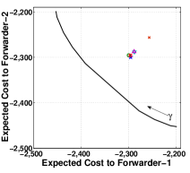
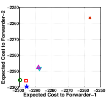
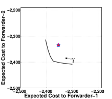
Figure 3: Performance of the various NEPPs and PO-NEPPs are depicted as points in $\Re^{2}$ where the first (second) coordinate is the expected cost incurred by $\mathscr{F}_{1}$ ($\mathscr{F}_{2}$). Fig. 3 corresponds to the case when the distance of separation $\theta=0$ m. A portion of Fig. 3 is enlarged and shown in Fig. 3. Fig. 3 corresponds to $\theta=10$ m.

VIII-A One-Hop Study

The one-hop study can be more general, requiring only a joint p.m.f. $p_{i,j}$, a location p.m.f. $q_{\ell}$, and conditional p.m.f.s $p^{(1)}_{i|\ell}$ and $p_{j|\ell}^{(2)}$ (for all $i,j$ and $\ell$). However, to illustrate the practicality of our study, we will study the geographical forwarding example described in Section III.

Recall the packet forwarding scenario illustrated in Fig. 1. We will fix the locations of $\mathscr{F}_{1}$ and $\mathscr{F}_{2}$ to be $v_{1}=[0,\frac{\theta}{2}]$ and $v_{2}=[0,-\frac{\theta}{2}]$, respectively. Thus, the distance of separation between the two forwarders is $\theta$ meters (m); we will vary $\theta$ and study the performance of the various policies. The range of each forwarder is $d=80$ m. The combined forwarding region is discretized into a uniform grid where the distance between the neighboring points is $5$ m. Finally, the sink node is placed at $v_{0}=[1000,0]$.

Next, recall the power and reward expressions from (5) and (8), respectively. We have fixed $d_{ref}=5$ m, $\xi=2.5$, and $a=0.5$. For $\Gamma N_{0}$, which is referred to as the receiver sensitivity, we use a value of $10^{-9}$ milliWatts (mW) (equivalently $-90$ dBm) specified for the Crossbow TelosB wireless mote [43]. The maximum transmit power available at a node is $P_{max}=1$ mW (equivalently $0$ dBm; again from the Crossbow TelosB data sheet). We allow for four different channel gain values: $0.4\times 10^{-3}$, $0.6\times 10^{-3}$, $0.8\times 10^{-3}$, and $1\times 10^{-3}$, each occurring with equal probability. Finally, we fix $\eta_{1}=\eta_{2}=100$ (recall that $\eta_{\rho}$ is the parameter used to trade-off between delay and reward (see (2)), $\nu_{1}=1-\nu_{2}=0.5$ ($\nu_{\rho}$ is the probability that $F_{\rho}$ will win the contention), and the mean inter-wake-up time $\tau=10$ milliseconds (ms).

We first set $\theta=0$ m (recall that $\theta$ is the distance between the two forwarders) and, in Fig. 3, depict the performance of various NEPPs and PO-NEPPs as pair of costs $\mathbf{C}=(C^{(1)},C^{(2)})$ where $C^{(\rho)}$ is the cost incurred by $F_{\rho}$ starting from time $0$ if the particular NEPP or PO-NEPP is used. Also shown in Fig. 3 is the performance of a simple policy (the point marked $\times$; to be describe next) along with the Pareto optimal boundary (the solid curve). Since, from Fig. 3 it is not easy to distinguish between the various points, we show a section of Fig. 3 as Fig. 3. Fig. 3 corresponds to $\theta=10$ m.

Various Policy Pairs: The description of various points seen in Fig. 3 is as follows (we will use $\mathbf{C}_{symbol}$ to denote the cost pair corresponding to the policy $symbol$):

• ${\bigstar}$,$\bigcirc$,and $\Box$: performances of the NEPPs that uses the NE strategies $(\textsf{s},\textsf{c})$, $(\textsf{c},\textsf{s})$, and the mixed strategy $(\Gamma_{1},\Gamma_{2})$, respectively, whenever $(r_{i},r_{j})\in\mathcal{R}_{4}(\mathbf{C}_{\bigstar})$, $\mathcal{R}_{4}(\mathbf{C}_{\bigcirc})$,and $\mathcal{R}_{4}(\mathbf{C}_{\Box})$, respectively (recall Fig. 2).

• $\nabla$ and $\Delta$: performances of the PO-NEPPs that are constructed by choosing, for each $\ell\in\mathcal{L}$, the thresholds $(\Phi_{\ell,1},\Psi_{\ell,N})$ and $(\Phi_{\ell,N},\Psi_{\ell,1})$, respectively (recall the proof of Theorem 4).

• $\times$: performance of a simple policy where each forwarder $\mathscr{F}_{\rho}$ ($\rho=1,2$) chooses s if and only if its reward value $r_{\rho}\geq\alpha^{(\rho)}$. Such a policy is optimal whenever $\mathscr{F}_{\rho}$ is alone in the system (recall (25) and (30)). Thus, using the simple policy each forwarder behaves as if the competing forwarder is not present.

• solid curve: Pareto optimal boundary obtained by $(\pi_{1}^{\gamma},\pi_{2}^{\gamma})$, $\gamma\in(0,1)$; recall Section VII.

Observations: From Fig. 3 we see that operating at NEPP $\bigstar$ is most favorable for $\mathscr{F}_{2}$ since $C_{\bigstar}^{(2)}$ is less than the cost to $\mathscr{F}_{2}$ at the other two NEPPs, $C^{(2)}_{\bigcirc}$ and $C^{(2)}_{\Box}$. This is because whenever $(r_{i},r_{j})\in\mathcal{R}_{4}(\mathbf{C}_{\bigstar})$ the joint-action $(\textsf{s},\textsf{c})$ played by $\bigstar$ fetches the least cost (of $D^{(2)}$) possibly by any strategy. In contrast, $\mathscr{F}_{1}$ incurs highest cost (of $-\eta_{1}r_{i}$) possible because of which NEPP $\bigstar$ is least favorable for $\mathscr{F}_{1}$. For a similar reason, operating at NEPP $\bigcirc$ is most favorable for $\mathscr{F}_{1}$ while being least favorable for $\mathscr{F}_{2}$. The NEPP ${\Box}$ which chooses the mixed strategy $(\Gamma_{1},\Gamma_{2})$ whenever $(r_{i},r_{j})\in\mathcal{R}_{4}(\mathbf{C}_{\Box})$ helps to achieve a fairer cost to both players, however the performance at $\Box$ is slightly farther from the Pareto boundary when compared with the other two NEPPs.

The performance at the PO-NEPPs, $\nabla$ and $\Delta$, is worse than at the NEPPs thus exhibiting the loss in performance due to partial information. The PO-NEPP $\nabla$ which uses the NE vector corresponding to the lowest-highest best response pair, $(\Phi_{\ell,1},\Psi_{\ell,N})$ (for each $\ell\in\mathcal{L}$), provides lower cost to $\mathscr{F}_{2}$ than the PO-NEPP $\Delta$. This is because, $\mathscr{F}_{1}$ using a lower threshold will essentially choose an initial relay, thus leaving $\mathscr{F}_{2}$ alone in the system which can now accrue a better cost. For a similar reason, operating at $\Delta$ leads to $\mathscr{F}_{1}$ achieving a lower cost. Finally, the simple policy $\times$ has the worst performance in comparison with all other points, suggesting that it may not be wise to be operating using this policy pair. However, as we increase the value of $\theta$ the performance of the simple policy improves, and interestingly for $\theta=10$ m (which is only $12.5\%$ of the forwarders’ range of $80$ m) we observe that the various points are practically indistinguishable (note that the magnitude of the scales in plots Fig. 3 and 3 is the same). We have observed similar trend when $\eta_{1}=\eta_{2}$ and $a$ are set to different values.

Key Insight: Thus, based on our numerical work we draw the following key insight: even for a small distance of separation between the forwarders, using the simple policy pair (where each forwarder behaves as if it is alone in the system) yields little (or, practically, no) loss in performance when compared with the performance of an NEPP or a PO-NEPP; however the performance degradation of the simple policy is significant whenever the forwarders are very close to each other. These observations are for the case where there are two forwarders. However, we expect a similar behavior for the simple policy even if there are more than two forwarders, i.e., we believe that the simple policy performs well if the competing forwarders are moderately separated.

VIII-B End-to-End Study

Finally, in this section we use simulation to provide an evaluation of the end-to-end performance of local forwarding. The competitive forwarding policies (i.e., NEPP and PO-NEPP) are difficult to implement since their structure has to be evaluated for each forwarding instance along the path of a packet. However, based on our observations in the previous section, we study the performance of the simple policy pair. In our prior work we have already studied the simple policy’s performance (see [4, Fig. 8] where the simple policy is referred to as SF), but there the setting was that of the lone packet model where a single alarm packet is generated which is then routed to the sink. Here, we will generalize the lone packet setting by generating multiple packets simultaneously across the network so that a packet, along its route, might have to compete with other packets in its vicinity before reaching the sink.

We first form a network by randomly placing $1000$ nodes in a square region of area $1$ Km². A source node is placed at $[0,1000]$ followed by a sink node at the diagonally opposite corner $[1000,0]$. Each node is allowed to asynchronously and periodically sleep-wake cycle with period $T=100$ ms, i.e., each node $i$ wakes up and stays ON for a small duration (which we neglect, given the other time scales) at the periodic instants $T_{i}+kT$, $k\geq 1$ where $\{T_{i}\}$ are i.i.d. uniform on $[0,T]$ (recall the discussion on the sleep-wake process from Section II).

Each node $i$, assuming an inter-wake-up time of ${1}/{N_{i}}$ (where $N_{i}$ is the average number of nodes in the forwarding region of node $i$), obtains $\alpha_{i}$ which is the threshold (on reward) required to implement the simple policy by node $i$. The values of all the other parameters required to compute the threshold, e.g., $P_{max}$, $\xi$, etc., remain the same as in our one-hop study. If there is no relay whose reward value is more than $\alpha_{i}$ (node $i$ will know of this after waiting for one entire duty-cycling period $T$), node $i$, at time $T$, will simply forward the packet to the relay with the maximum reward (thus, as relays wake-up the best relay so far, is asked to wait).

The source node generates an alarm packet at time $0$. We introduce competition by generating additional packets at randomly chosen nodes, randomly in time at the points of a Poisson process of rate $\lambda$. All the packets are destined for the same sink. While forwarding, if a relay is chosen simultaneously by more than one forwarder, then randomly one of them will win the contention and gets the relay to forward its packet to. We are interested in studying, as a function of $\lambda$, the performance obtained (in terms of end-to-end delay and the total power expended) in routing the source’s packet.

In Fig. 4 we have plotted, for different values of $\lambda$, the mean end-to-end delay vs. the mean end-to-end power (averaged over packets from the source located at $(0,1000)$). These curves are obtained by varying $\eta$, the parameter used to trade-off between delay and reward in the local problem. Each data point in Fig. 4 is the average of the respective quantities over $100$ alarm packets generated by the source node. Also shown in the figure is the performance curve corresponding to the “lone packet case” where no additional packets are generated. Hence the lone packet curve is analogous to the SF policy’s performance curves in [4, Fig. 8].

Observe that, as we increase $\lambda$ we obtain a degradation in performance, i.e., increased delay and power compared with the lone packet case. This is because, as $\lambda$ increases, since there are more packets in the network, there is a larger probability that a forwarding node carrying the source’s packet has to compete with other packets in the process of acquiring a relay. Also, as $\lambda$ increases, at these instances of competition, the competing nodes tend to be closer together. From the observations in the previous section, we can conclude that as $\lambda$ increases the performance of the simple policy will progressively degrade. However, the performance degradation is only marginal when the packet rate $\lambda\leq 20$ packets/sec while being moderate for $\lambda=30$ packets/sec, thus supporting the usage of the simple policy for these packet rates. For higher values of $\lambda$ (e.g., $\lambda=40$ packets/sec and beyond) the performance degradation is significant and hence there could be a benefit in using NEPPs to forward packets for these rates.

Finally, we have only presented simulation results for the simple policy, since implementing NEPPs or PO-NEPPs for end-to-end routing has the following difficulties: (1) for a given pair of neighboring nodes, obtaining NEPPs will require fixed point iterations, (2) NEPPs are node pair dependent, so that all possible neighboring node pairs are required to compute the corresponding NEPPs, since during actual forwarding a node may be competing with any of its neighbors. Thus, there is a large complexity involved in implementing NEPPs. In contrast, the simple policy (being a single threshold based) is easy to implement. Moreover, for realistic parameter values corresponding to TelosB wireless mote, we have seen that the performance of simple policy is good (in comparison with the lone packet case) for packet rates $\lambda\leq 30$ packets/sec.

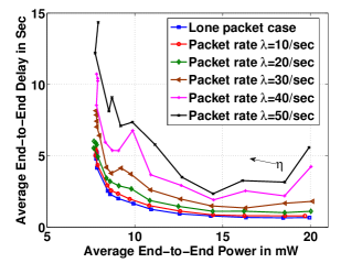
Figure 4: End-to-end performance (average power vs. average delay) of the simple policy as the competing packet rate $\lambda$ in the network is increased.

IX Conclusion

We studied the problem of competitive relay selection when two forwarders compete for a next-hop relay (or some resource in general). We first considered the model where complete information is available to both the forwarders. We formulated the problem as a stochastic game and proceeded to obtain solution in terms of Nash equilibrium policy pairs (NEPPs). We were able to provide insight into the structure of NEPPs, which was primarily possible because of our following key result (Lemma 2): “cost of continuing alone” is less than the “cost of continuing along with a competing forwarder”. We next studied a partially observable case for which we constructed a Bayesian game which is effective played at each stage. For this Bayesian game, we proved the existence of a Nash equilibrium strategy within the class of (pure) threshold vectors (Theorem 4). The proof method of this result enabled us to construct NEPPs for the partial case. For the geographical forwarding example, through numerical experiments we observed that, even for moderate separation between the two forwarders, the performance of our simple policy is as good as the performance of any other NEPP/PO-NEPP. In the context of end-to-end forwarding, through simulations we established (for the considered setting) that for packet rates less than $30$ packets/second, the performance of the simple policy is good compared with the lone packet case.

Appendix A Proof of Lemma 1

For convenience, here in the appendix we will recall the respective Lemma/Theorem statement before providing its proof.

Lemma 1: $\alpha^{(1)}$ is the unique fixed point of $\beta^{(1)}(x)$ ($x\in(-\infty,r_{n}]$) in (26).

Proof:

Let us recall the expression of $\beta^{(1)}(x)$:

$$\beta^{(1)}(x) = \mathbb{E}\Big{[}\max\{x,R_{1}\}\Big{]}-\frac{\tau}{\eta_{1}},$$

where the expection is w.r.t. the p.m.f. $p^{(1)}$ of $R_{1}$ (recall that $R_{1}$ takes values from the set $\{r_{1},r_{2},\cdots,r_{n}\}$).

Let $m=\max\{i\in[n]:p^{(1)}_{i}>0\}$. For $x>r_{m}$, note that $\beta^{(1)}(x)=x-\frac{\tau}{\eta_{1}}<x$. Hence a fixed point, if any, should lie within $(-\infty,r_{m}]$. Let us restrict $\beta^{(1)}(\cdot)$ to the domain $(-\infty,r_{m}]$. Then, since $\beta^{(1)}(x)\leq r_{m}$ for any $x\in(-\infty,r_{m}]$, we have $\beta^{(1)}:(-\infty,r_{m}]\rightarrow(-\infty,r_{m}]$. We can now proceed to show that $\beta^{(1)}(x)$ restricted to $x\in(-\infty,r_{m}]$ is a contraction mapping, i.e., for any $x,x^{\prime}\in(-\infty,r_{m}]$, we need to show that

$$\parallel\beta^{(1)}(x)-\beta^{(1)}(x^{\prime})\parallel\leq\kappa\parallel x-x^{\prime}\parallel$$ (62)

for some $\kappa<1$. Without loss of generality let $x>x^{\prime}$. Then,

$$\parallel\beta^{(1)}(x)-\beta^{(1)}(x^{\prime})\parallel = \beta^{(1)}(x)-\beta^{(1)}(x^{\prime})$$

$$= \mathbb{E}\Big{[}\max\{x,R_{1}\}\Big{]}-\mathbb{E}\Big{[}\max\{x^{\prime},R_{1}\}\Big{]}$$

$$= \sum_{i=1}^{n}p^{(1)}_{i}\Big{(}\max\{x,r_{i}\}-\max\{x^{\prime},r_{i}\}\Big{)}$$

$$\overset{*}{=} \sum_{i=1}^{m}p^{(1)}_{i}\Big{(}\max\{x,r_{i}\}-\max\{x^{\prime},r_{i}\}\Big{)}$$

$$\overset{o}{=} \sum_{i=1}^{m-1}p^{(1)}_{i}\Big{(}\max\{x,r_{i}\}-\max\{x^{\prime},r_{i}\}\Big{)}$$

$$\overset{\dagger}{\leq} \sum_{i=1}^{m-1}p^{(1)}_{i}\Big{(}x-x^{\prime}\Big{)}$$

$$= (1-p^{(1)}_{m})\parallel x-x^{\prime}\parallel.$$

In the above derivation, $*$ is because $p_{i}^{(1)}=0$ for $i>m$ (recall the definition of $m$); $o$ is because, since $x,x^{\prime}\leq r_{m}$, we have $\Big{(}\max\{x,r_{m}\}-\max\{x^{\prime},r_{m}\}\Big{)}=0$; to obtain $\dagger$ note that, $\Big{(}\max\{x,r_{i}\}-\max\{x^{\prime},r_{i}\}\Big{)}\leq(x-x^{\prime})$ for any $r_{i}$. Thus, $\beta^{(1)}(x)$, $x\in(-\infty,r_{m}]$ is a contraction mapping (recall 62) with $\kappa=(1-p^{(1)}_{m})<1$ (since $p^{(1)}_{m}>0$ from definition). Hence from the Banach fixed point theorem [38] it follows that there exists a unique fixed point $\alpha^{*}\in(-\infty,r_{m}]$, i.e., $\alpha^{*}$ satisfies $\alpha^{*}=\beta^{(1)}(\alpha^{*})$.

Now, suppose we can show that

$$J^{(1)}_{\pi_{1}^{*},\pi_{2}^{*}}(r_{i},\textbf{\emph{t}})=\min\Big{\{}-\eta_{1}r_{i},-\eta_{1}\alpha^{*}\Big{\}}$$ (63)

then, recalling the expression for $D^{(1)}$ from (22), we obtain

$$\alpha^{(1)} = \frac{D^{(1)}}{-\eta_{1}}$$

$$= -\frac{\tau}{\eta_{1}}-\frac{1}{\eta_{1}}\sum_{i}p^{(1)}_{i}J^{(1)}_{\pi_{1}^{*},\pi_{2}^{*}}(r_{i},\textbf{\emph{t}})$$

$$= \mathbb{E}\Big{[}\max\{\alpha^{*},R_{1}\}\Big{]}-\frac{\tau}{\eta_{1}}.$$

$$= \beta^{(1)}(\alpha^{*})$$

$$= \alpha^{*}.$$

Thus, $\alpha^{(1)}$ is the unique fixed point of $\beta^{(1)}(\cdot)$.

To show (63), we proceed as follows. Let $J_{0}(r_{i})=0$ for all $r_{i}$, and for $k\geq 1$ define $J_{k}(r_{i})$ inductively as

$$J_{k}(r_{i}) = \min\Big{\{}-\eta_{1}r_{i},\tau+\mathbb{E}\Big{[}J_{k-1}(R_{1})\Big{]}\Big{\}}.$$ (64)

Since our problem with one player is equivalent to the optimal stopping problem studied in [39], the above iterations converge to the optimal cost, i.e., $\lim_{k\rightarrow\infty}J_{k}(r_{i})=J^{(1)}_{\pi_{1}^{*},\pi_{2}^{*}}(r_{i},\textbf{\emph{t}})$. Now, defining $\alpha_{1}=-\frac{\tau}{\eta_{1}}$, $J_{1}(r_{i})$ can be written as $J_{1}(r_{i})=\min\{-\eta_{1}r_{i},-\eta_{1}\alpha_{1}\}$. Proceeding further we can write,

$$J_{2}(r_{i}) = \min\Big{\{}-\eta_{1}r_{i},\tau+\mathbb{E}\Big{[}J_{1}(R_{1})\Big{]}\Big{\}}$$

$$= \min\Big{\{}-\eta_{1}r_{i},\tau+\mathbb{E}\Big{[}\min\{-\eta_{1}\alpha_{1},-\eta_{1}R\}\Big{]}\Big{\}}$$

$$= \min\Big{\{}-\eta_{1}r_{i},-\eta_{1}\beta^{(1)}(\alpha_{1})\Big{\}}$$

$$= \min\Big{\{}-\eta_{1}r_{i},-\eta_{1}\alpha_{2}\Big{\}}$$

where $\alpha_{2}=\beta^{(1)}(\alpha_{1})$. Similarly it can be shown that, if $J_{k-1}(r_{i})=\min\Big{\{}-\eta_{1}r_{i},-\eta_{1}\alpha_{k-1}\Big{\}}$, then

$$J_{k}(r_{i})=\min\Big{\{}-\eta_{1}r_{i},-\eta_{1}\alpha_{k}\Big{\}}$$ (65)

where $\alpha_{k}=\beta^{(1)}(\alpha_{k-1})$. Thus $\alpha_{k}\rightarrow\alpha^{*}$. Finally, in the above expression taking the limit as $k\rightarrow\infty$ on both sides, and using $J_{k}(r_{i})\rightarrow J^{(1)}_{\pi_{1}^{*},\pi_{2}^{*}}(r_{i},\textbf{\emph{t}})$ and $\alpha_{k}\rightarrow\alpha^{*}$, we obtain the desired result. ∎

Appendix B Proof of Theorem 1

Theorem 1: Given a policy pair, $(\pi_{1}^{*},\pi_{2}^{*})$, construct the static game given in Table 5.

	c	s
c	$C^{(1)}_{\pi_{1}^{*},\pi_{2}^{*}},C^{(2)}_{\pi_{1}^{*},\pi_{2}^{*}}$	$D^{(1)},-\eta_{2}r_{j}$
s	$-\eta_{1}r_{i},D^{(2)}$	$E^{(1)}(r_{i}),E^{(2)}(r_{j})$

TABLE 5: Static stage game.

Then the following statements are equivalent:

1. $(\pi_{1}^{*},\pi_{2}^{*})$ is an NEPP.

2. For any $x=(r_{i},r_{j})$, $(\pi_{1}^{*}(x),\pi_{2}^{*}(x))$ is a Nash equilibrium (NE) strategy for the game in Table 5. Further, the expected cost pair at this NE strategy is, $(J^{(1)}_{\pi_{1}^{*},\pi_{2}^{*}}(x),J^{(2)}_{\pi_{1}^{*},\pi_{2}^{*}}(x))$.

Proof:

Suppose (a) is true, i.e., $(\pi_{1}^{*},\pi_{2}^{*})$ is an NEPP. Then, $\pi_{1}^{*}$ is the best response policy of $\mathscr{F}_{1}$ against the policy $\pi_{2}^{*}$ of $\mathscr{F}_{2}$. Hence $\pi_{1}^{*}$ is optimal for the MDP problem, denoted $MDP_{1}(\pi_{2}^{*})$, which is obtained by fixing the policy $\pi_{2}^{*}$ of $\mathscr{F}_{2}$ (note that $MDP_{1}(\pi_{2}^{*})$ is a time homogeneous MDP since $\pi_{2}^{*}$ is stationary; recall Definition 1). Since (1) the states of the form $(\textbf{\emph{t}},r_{j})$ are absorbing and cost free for $\mathscr{F}_{1}$, and (2) the policy of $\mathscr{F}_{1}$ which never stops incurs infinite cost to $\mathscr{F}_{1}$, it follows that $MDP_{1}(\pi_{2}^{*})$ is an optimal stopping problem [39]. Hence, $J^{(1)}_{\pi_{1}^{*},\pi_{2}^{*}}(x)$, $x=(r_{i},r_{j})$ satisfies the following Bellman equation,

$$J^{(1)}_{\pi_{1}^{*},\pi_{2}^{*}}(x) = \min\Big{\{}C_{\textsf{s}}(x),C_{\textsf{c}}(x)\Big{\}}$$ (66)

$$= \min\Big{\{}\pi_{2}^{*}(x,\textsf{c})(-\eta_{1}r_{i})+\pi_{2}^{*}(x,\textsf{s})E^{(1)}(r_{i}),$$

$$\hskip 113.81102pt\pi_{2}^{*}(x,\textsf{c})C^{(1)}_{\pi_{1}^{*},\pi_{2}^{*}}+\pi_{2}^{*}(x,\textsf{s})D^{(1)}\Big{\}},$$

where $\pi_{2}^{*}(x,\textsf{c})$ (resp. $\pi_{2}^{*}(x,\textsf{s})$) is the probability that $\mathscr{F}_{2}$ will choose action c (resp. s) when the state is $x$. The two terms in the $\min$-expression above (denoted $C_{\textsf{s}}(x)$ and $C_{\textsf{c}}(x)$) are the expected cost to $\mathscr{F}_{1}$ for taking actions s and c, respectively. Note that these costs are exactly the expected cost incurred by $\mathscr{F}_{1}$, for playing actions s and c, respectively, in the static game in Table 4, when the strategy of $\mathscr{F}_{2}$ is $\pi_{2}^{*}(x)$. Now $\pi_{1}^{*}$, being optimal for $MDP_{1}(\pi_{2}^{*})$, chooses action $\pi_{1}^{*}(x)\in\Delta(\{\textsf{s},\textsf{c}\})$ whichever gives a minimum cost or can randomize between the two if both the costs are equal. Hence, it follows from the structure of (66) that $\pi_{1}^{*}(x)$ is the best response against $\pi_{2}^{*}(x)$ for the game in Table 4. Further the cost to $\mathscr{F}_{1}$ for playing $\pi_{1}^{*}(x)$, from Table 4, is $\min\{C_{\textsf{s}}(x),C_{\textsf{c}}(x)\}=J^{(1)}_{\pi_{1}^{*},\pi_{2}^{*}}(x)$.

Similarly, by writing the Bellman equation corresponding to the $MDP_{2}(\pi_{1}^{*})$ problem (which is obtained by fixing the policy $\pi_{1}^{*}$ of $\mathscr{F}_{1}$), we can conclude that $\pi_{2}^{*}(x)$ is the best response against $\pi_{1}^{*}(x)$ for the game in Table 4, with the cost to player $\mathscr{F}_{2}$ being $J^{(2)}_{\pi_{1}^{*},\pi_{2}^{*}}(x)$.

Proof of (b)$\implies$(a): Given that the policy $(\pi_{1}^{*},\pi_{2}^{*})$ satisfies the condition in (b), let $\pi_{1}$ be any policy of $\mathscr{F}_{1}$. Then, for any $x=(r_{i},r_{j})$, since $(\pi_{1}^{*}(x),\pi_{2}^{*}(x))$ is a NE strategy for the game in Table 4 with cost to $\mathscr{F}_{1}$ at equilibrium being $J^{(1)}_{\pi_{1}^{*},\pi_{2}^{*}}(x)$, we can write

$$J^{(1)}_{\pi_{1}^{*},\pi_{2}^{*}}(x) \leq \pi_{1}(x,\textsf{c})\Big{(}\pi_{2}^{*}(x,\textsf{c})C^{(1)}_{\pi_{1}^{*},\pi_{2}^{*}}+\pi_{2}^{*}(x,\textsf{s})D^{(1)}\Big{)}+$$

$$\hskip 56.9055pt\pi_{1}(x,\textsf{s})\Big{(}\pi_{2}^{*}(x,\textsf{c})(-\eta_{1}r_{i})+\pi_{2}^{*}(x,\textsf{s})E^{(1)}(r_{i})\Big{)}.$$

LHS of the above expression is the cost incurred to $\mathscr{F}_{1}$ when the strategy played is $(\pi_{1}(x),\pi_{2}^{*}(x))$ (refer to (66)).

Substituting for $D^{(1)}$, $E^{(1)}(r_{i})$ and $C^{(1)}_{\pi_{1}^{*},\pi_{2}^{*}}$, (from (22), (31) and (33), respectively) in the above expression and then rearranging, we can write

$$J^{(1)}_{\pi_{1}^{*},\pi_{2}^{*}}(x) \leq \mathbb{E}_{\pi_{1},\pi_{2}^{*}}^{x}\Big{[}g_{1}(X_{1},(A_{1,1},A_{2,1}))\Big{]}+\mathbb{E}_{\pi_{1},\pi_{2}^{*}}^{x}\Big{[}J^{(1)}_{\pi_{1}^{*},\pi_{2}^{*}}(X_{2})\Big{]}$$

Observe that, $J^{(1)}_{\pi_{1}^{*},\pi_{2}^{*}}(\cdot)$ appears on the RHS of the above expression. Hence, inductively applying the above inequality $K$ times, we obtain

$$J^{(1)}_{\pi_{1}^{*},\pi_{2}^{*}}(x) \leq \sum_{k=1}^{K}\mathbb{E}_{\pi_{1},\pi_{2}^{*}}^{x}\Big{[}g_{1}(X_{k},(A_{1,k},A_{2,k}))\Big{]}+\mathbb{E}_{\pi_{1},\pi_{2}^{*}}^{x}\Big{[}J^{(1)}_{\pi_{1}^{*},\pi_{2}^{*}}(X_{K+1})\Big{]}$$

Taking limit as $K\rightarrow\infty$ in the above expression we obtain,

$$J^{(1)}_{\pi_{1}^{*},\pi_{2}^{*}}(x)\leq J^{(1)}_{\pi_{1},\pi_{2}^{*}}(x)+\lim_{K\rightarrow\infty}\mathbb{E}_{\pi_{1},\pi_{2}^{*}}^{x}\Big{[}J^{(1)}_{\pi_{1}^{*},\pi_{2}^{*}}(X_{K+1})\Big{]}.$$ (67)

Now, let $\mathcal{A}_{\textbf{\emph{t}}}=\{(\textbf{\emph{t}},\textbf{\emph{t}})\}\cup\{(\textbf{\emph{t}},r_{j}):j\in[n]\}$. $\mathcal{A}_{\textbf{\emph{t}}}$ is the set of all states, which are entered once $\mathscr{F}_{1}$ terminates. We will assume that the policy pair $(\pi_{1},\pi_{2}^{*})$ is such that $\mathscr{F}_{1}$ will eventually terminate starting from any state $x$, i.e., $\lim_{K\rightarrow\infty}\mathbb{P}_{\pi_{1},\pi_{2}^{*}}^{x}(X_{K}\in\mathcal{A}_{\textbf{\emph{t}}})=1$, or equivalently, for any $x^{\prime}\notin\mathcal{A}_{\textbf{\emph{t}}}$, $\lim_{K\rightarrow\infty}\mathbb{P}_{\pi_{1},\pi_{2}^{*}}^{x}(X_{K}=x^{\prime})=0$ (otherwise, with positive probability $\mathscr{F}_{1}$ will continue forever incurring a delay cost of $\tau$ at every stage yielding $J^{(1)}_{\pi_{1}^{*},\pi_{2}^{*}}(x)=\infty$, so that the inequality $J^{(1)}_{\pi_{1}^{*},\pi_{2}^{*}}(x)\leq J^{(1)}_{\pi_{1},\pi_{2}^{*}}(x)$ trivially holds). Using this along with $J^{(1)}_{\pi_{1}^{*},\pi_{2}^{*}}(x^{o})=0$ for any $x^{o}\in\mathcal{A}_{\textbf{\emph{t}}}$, we can write

$${\lim_{K\rightarrow\infty}\mathbb{E}_{\pi_{1},\pi_{2}^{*}}^{x}\Big{[}J^{(1)}_{\pi_{1}^{*},\pi_{2}^{*}}(X_{K+1})\Big{]}} = \lim_{K\rightarrow\infty}\Bigg{(}\sum_{x^{o}\in\mathcal{A}_{\textbf{\emph{t}}}}\mathbb{P}_{\pi_{1},\pi_{2}^{*}}^{x}(X_{K+1}=x^{o})J^{(1)}_{\pi_{1}^{*},\pi_{2}^{*}}(x^{o})+$$

$$\hskip 85.35826pt\sum_{x^{\prime}\notin\mathcal{A}_{\textbf{\emph{t}}}}\mathbb{P}_{\pi_{1},\pi_{2}^{*}}^{x}(X_{K+1}=x^{\prime})J^{(1)}_{\pi_{1}^{*},\pi_{2}^{*}}(x^{\prime})\Bigg{)}$$

$$\overset{*}{=} \sum_{x^{\prime}\notin\mathcal{A}_{\textbf{\emph{t}}}}\lim_{K\rightarrow\infty}\Big{(}\mathbb{P}_{\pi_{1},\pi_{2}^{*}}^{x}(X_{K+1}=x^{\prime})J^{(1)}_{\pi_{1}^{*},\pi_{2}^{*}}(x^{\prime})\Big{)}$$

$$\overset{o}{=} \sum_{x^{\prime}\notin\mathcal{A}_{\textbf{\emph{t}}}}\Big{(}\lim_{K\rightarrow\infty}\mathbb{P}_{\pi_{1},\pi_{2}^{*}}^{x}(X_{K+1}=x^{\prime})\Big{)}\ J^{(1)}_{\pi_{1}^{*},\pi_{2}^{*}}(x^{\prime})$$

$$= 0.$$

Note that, in $*$ interchanging the limit and summation was possible because we have a finite sum (since our state space is finite). Also, since we have restricted ourselves to the class of stationary policies (recall Definition 1), $J^{(1)}_{\pi_{1}^{*},\pi_{2}^{*}}(x^{\prime})$ is not a function of the stage index $K$, which enables us to proceed to $o$. Finally, using the above in (67) we obtain, $J^{(1)}_{\pi_{1}^{*},\pi_{2}^{*}}(x)\leq J^{(1)}_{\pi_{1},\pi_{2}^{*}}(x)$.

Similarly, for $\mathscr{F}_{2}$ it can be shown that $J^{(2)}_{\pi_{1}^{*},\pi_{2}^{*}}(x)\leq J^{(2)}_{\pi_{1}^{*},\pi_{2}}(x)$ for any $\pi_{2}$ and $x=(r_{i},r_{j})$. ∎

Appendix C Proof of Lemma 2

Lemma 2 will be an immediate consequence of the following result.

Lemma 7

Given an NEPP $(\pi_{1}^{*},\pi_{2}^{*})$, for any $(r_{i},r_{j})\in\mathcal{X}$ we have,

$$J^{(1)}_{\pi_{1}^{*},\pi_{2}^{*}}(r_{i},\textbf{\emph{t}}) \leq J^{(1)}_{\pi_{1}^{*},\pi_{2}^{*}}(r_{i},r_{j}),$$ (68)

$$J^{(2)}_{\pi_{1}^{*},\pi_{2}^{*}}(\textbf{\emph{t}},r_{j}) \leq J^{(2)}_{\pi_{1}^{*},\pi_{2}^{*}}(r_{i},r_{j}).$$ (69)

Proof:

We will prove only (68); the proof of (69) is along similar lines. Since $(\pi_{1}^{*},\pi_{2}^{*})$ is an NEPP, it follows that the policy $\pi_{1}^{*}$ is the best response for $\mathscr{F}_{1}$ against the policy $\pi_{2}^{*}$ of $\mathscr{F}_{2}$, i.e., for any $x\in\mathcal{X}$, $J^{(1)}_{{\pi}_{1}^{*},\pi_{2}^{*}}(x)=\inf_{\pi_{1}}J^{(1)}_{\pi_{1},\pi_{2}^{*}}(x)$. Thus $J^{(1)}_{{\pi}_{1}^{*},\pi_{2}^{*}}(x)$ can be regarded as the optimal cost of the MDP problem, $MDP_{1}(\pi_{2}^{*})$, obtained by fixing the policy $\pi_{2}^{*}$ of $\mathscr{F}_{2}$. For simplicity of notation we will denote $J^{(1)}_{{\pi}_{1}^{*},\pi_{2}^{*}}(x)$ as $H^{*}(x)$. Thus for the states of the form $(r_{i},\textbf{\emph{t}})$, $H^{*}(r_{i},\textbf{\emph{t}})$ satisfies the following Bellman equation (this expression is same as the one in (21))

$$H^{*}(r_{i},\textbf{\emph{t}})=\min\Big{\{}-\eta_{1}r_{i},C_{\textsf{c}}(r_{i},\textbf{\emph{t}})\Big{\}},$$ (70)

where

$$C_{\textsf{c}}(r_{i},\textbf{\emph{t}})=\tau+\sum_{i^{\prime}}p^{(1)}_{i^{\prime}}H^{*}(r_{i^{\prime}},\textbf{\emph{t}})$$ (71)

is the expected cost of continuing, and $-\eta_{1}r_{i}$ is the cost of stopping.

However, for states of the form $(r_{i},r_{j})$ (where $\mathscr{F}_{2}$ is also competing for a relay), the optimality equation is more involved since the actions of $\mathscr{F}_{2}$ will now affect both costs (stopping and continuing) of $\mathscr{F}_{1}$. Defining $\epsilon=\pi_{2}^{*}(r_{i},r_{j},\textsf{s})$ ($\epsilon$ is the probability with which $\mathscr{F}_{2}$ will stop when the state is $(r_{i},r_{j})$), Bellman equation for states of the form $(r_{i},r_{j})$ can be written as

$$H^{*}(r_{i},r_{j})=\min\Big{\{}C_{\textsf{s}}(r_{i},r_{j}),C_{\textsf{c}}(r_{i},r_{j})\Big{\}},$$ (72)

where $C_{\textsf{s}}(r_{i},r_{j})$ is the expected cost incurred by $\mathscr{F}_{1}$ for stopping when the state is $(r_{i},r_{j})$, and $C_{\textsf{c}}(r_{i},r_{j})$ is the expected cost of continuing.

The expression for $C_{\textsf{s}}(r_{i},r_{j})$ is (recall that $\nu_{\rho}$, $\rho=1,2$, is the probability that $\mathscr{F}_{\rho}$ gets the relay if both forwarders simultaneously choose to stop),

$$C_{\textsf{s}}(r_{i},r_{j}) = \epsilon\Big{(}\nu_{1}(-\eta_{1}r_{i})+\nu_{2}C_{\textsf{c}}(r_{i},\textbf{\emph{t}})\Big{)}+(1-\epsilon)\Big{(}-\eta_{1}r_{i}\Big{)}.$$ (73)

The first term in the RHS of the above expression is the expected stopping cost incurred by $\mathscr{F}_{1}$ conditioned on the event that $\mathscr{F}_{2}$ also decides to stop. This can be understood as follows: suppose $\mathscr{F}_{2}$ also decides to stop (probability of which is $\epsilon$), then w.p. $\nu_{1}$, $\mathscr{F}_{1}$ gets the relay incurring a termination cost of $-\eta_{1}r_{i}$, otherwise $\mathscr{F}_{2}$ gets the relay in which case $\mathscr{F}_{1}$ has to continue alone, the expected cost of which is $C_{\textsf{c}}(r_{i},\textbf{\emph{t}})$. The remaining term, $(1-\epsilon)(-\eta_{1}r_{i})$, in (73) is the stopping cost incurred to $\mathscr{F}_{1}$ when the action of $\mathscr{F}_{2}$ is to continue (which happens with probability $(1-\epsilon)$).

Similarly, the cost incurred by $\mathscr{F}_{1}$ for continuing, $C_{\textsf{c}}(r_{i},r_{j})$, can be written as,

$$C_{\textsf{c}}(r_{i},r_{j}) = \epsilon\Big{(}\tau+\sum_{i^{\prime}}p^{(1)}_{i^{\prime}}H^{*}(r_{i^{\prime}},\textbf{\emph{t}})\Big{)}+(1-\epsilon)\Big{(}\tau+\sum_{i^{\prime},j^{\prime}}p_{i^{\prime},j^{\prime}}H^{*}(r_{i^{\prime}},r_{j^{\prime}})\Big{)}.$$ (74)

Now, returning to (70) and (72), $H^{*}$ can be expressed as the fixed point of a mapping $T$ which is, for a function $H(\cdot,\cdot)$, given by,

$$TH(r_{i},\textbf{\emph{t}}) = \min\Big{\{}-\eta_{1}r_{i},C_{\textsf{c}}^{H}(r_{i},\textbf{\emph{t}})\Big{\}}$$

$$TH(r_{1},r_{2}) = \min\Big{\{}C_{\textsf{s}}^{H}(r_{i},r_{j}),C_{\textsf{c}}^{H}(r_{i},r_{j})\Big{\}},$$

where the expressions for $C_{\textsf{c}}^{H}(r_{i},\textbf{\emph{t}})$, $C_{\textsf{s}}^{H}(r_{i},r_{j})$ and $C_{\textsf{c}}^{H}(r_{i},r_{j})$ is similar to that of $C_{\textsf{c}}(r_{i},\textbf{\emph{t}})$, $C_{\textsf{s}}(r_{i},r_{j})$ and $C_{\textsf{c}}(r_{i},r_{j})$ (in (71) (73) and (74), respectively) with $H^{*}$ replaced by the given function $H$. Inductively define $H_{k}=TH_{k-1}$ with $H_{0}\equiv 0$ (i.e., $H_{0}(x)=0$ for all $x\in\mathcal{X}$). Since $MDP_{1}(\pi_{2}^{*})$ is an optimal stopping problem [39] it follows that $H_{k}\rightarrow H^{*}$ (this is the value iteration algorithm). Hence, to complete the proof we will show that $H_{k}(r_{i},\textbf{\emph{t}})\leq H_{k}(r_{i},r_{j})$ whenever $H_{k-1}(r_{i},\textbf{\emph{t}})\leq H_{k-1}(r_{i},r_{j})$.

Suppose, for some $k\geq 1$, $H_{k-1}(r_{i},\textbf{\emph{t}})\leq H_{k-1}(r_{i},r_{j})$ for all $(r_{i},r_{j})\in\mathcal{X}$ (this holds trivially for $k=1$). First consider the case where, $-\eta_{1}r_{i}\leq C_{\textsf{c}}^{H_{k-1}}(r_{i},\textbf{\emph{t}})$ (i.e., it is optimal to stop when the state is $(r_{i},\textbf{\emph{t}})$).

• Then from (73) we obtain $-\eta_{1}r_{i}\leq C_{\textsf{s}}^{H_{k-1}}(r_{i},r_{j})$.

• Also, from the induction hypothesis we have

  $$\sum_{i^{\prime}}p^{(1)}_{i^{\prime}}H_{k-1}(r_{i^{\prime}},\textbf{\emph{t}}) = \sum_{i^{\prime},j^{\prime}}p_{i^{\prime},j^{\prime}}H_{k-1}(r_{i^{\prime}},\textbf{\emph{t}})$$

  $$\leq \sum_{i^{\prime},j^{\prime}}p_{i^{\prime},j^{\prime}}H_{k-1}(r_{i^{\prime}},r_{j^{\prime}}).$$

  Using the above in (74) and recalling (71) we can write

  $$C_{\textsf{c}}^{H_{k-1}}(r_{i},r_{j}) \geq \tau+\sum_{i^{\prime}}p^{(1)}_{i^{\prime}}H^{*}(r_{i^{\prime}},\textbf{\emph{t}})$$

  $$= C_{\textsf{c}}(r_{i},\textbf{\emph{t}})$$

  $$\geq -\eta_{1}r_{i}.$$

Thus we have,

$$H_{k}(r_{i},\textbf{\emph{t}}) = \min\Big{\{}-\eta_{1}r_{i},C_{\textsf{c}}^{H_{k-1}}(r_{i},\textbf{\emph{t}})\Big{\}}$$

$$= -\eta_{1}r_{i}$$

$$\leq \min\Big{\{}C_{\textsf{s}}^{H_{k-1}}(r_{i},r_{j}),C_{\textsf{c}}^{H_{k-1}}(r_{i},r_{j})\Big{\}}$$

$$= H_{k}(r_{i},r_{j}).$$

Similarly for the other case, i.e., when $-\eta_{1}r_{i}>C_{\textsf{c}}^{H}(r_{i},\textbf{\emph{t}})$, we can show that both the costs, $C_{\textsf{s}}^{H_{k-1}}(r_{i},r_{j})$ and $C_{\textsf{s}}^{H_{k-1}}(r_{i},r_{j})$, are less than $C_{\textsf{c}}^{H}(r_{i},\textbf{\emph{t}})$ again yielding $H_{k}(r_{i},\textbf{\emph{t}})\leq H_{k}(r_{i},r_{j})$. ∎

We are now ready to prove Lemma 2.

Lemma 2: For an NEPP, $(\pi_{1}^{*},\pi_{2}^{*})$, the various costs are ordered as follows:

$$D^{(1)}\leq C^{(1)}_{\pi_{1}^{*},\pi_{2}^{*}}\mbox{ and }D^{(2)}\leq C^{(2)}_{\pi_{1}^{*},\pi_{2}^{*}}.$$

Proof:

Recalling the cost expressions of $D^{(1)}$ and $C^{(1)}_{\pi_{1}^{*},\pi_{2}^{*}}$ (from (22) and (33), respectively) we can write,

$$D^{(1)} = \tau+\sum_{i^{\prime}}p^{(1)}_{i^{\prime}}J^{(1)}_{\pi_{1}^{*},\pi_{2}^{*}}(r_{i^{\prime}},\textbf{\emph{t}})$$

$$= \tau+\sum_{i^{\prime},j^{\prime}}p_{i^{\prime},j^{\prime}}J^{(1)}_{\pi_{1}^{*},\pi_{2}^{*}}(r_{i^{\prime}},\textbf{\emph{t}})$$

$$\overset{*}{\leq} \tau+\sum_{i^{\prime},j^{\prime}}p_{i^{\prime},j^{\prime}}J^{(1)}_{\pi_{1}^{*},\pi_{2}^{*}}(r_{i^{\prime}},r_{j^{\prime}})$$

$$= C^{(1)}_{\pi_{1}^{*},\pi_{2}^{*}},$$

where $*$ is due to Lemma 7. Similarly, one can show that $D^{(2)}\leq C^{(2)}_{\pi_{1}^{*},\pi_{2}^{*}}$. ∎

Appendix D Obtaining NE Strategies for the Static Game in Table 4

For convenience, let us first recall the game in Table 4.

	c	s
c	$C^{(1)}_{\pi_{1}^{*},\pi_{2}^{*}},C^{(2)}_{\pi_{1}^{*},\pi_{2}^{*}}$	$D^{(1)},-\eta_{2}r_{j}$
s	$-\eta_{1}r_{i},D^{(2)}$	$E^{(1)}(r_{i}),E^{(2)}(r_{j})$

TABLE 6: Static stage game.

Since only two actions (namely s and c) are available to each forwarder, a strategy used by $\mathscr{F}_{1}$ can be conveniently represented by $\sigma_{1}\in[0,1]$, where $\sigma_{1}$ is the probability that $\mathscr{F}_{1}$ will choose action s. Similarly, $\sigma_{2}\in[0,1]$ is the probability that $\mathscr{F}_{2}$ will choose action s. Given a strategy pair $(\sigma_{1},\sigma_{2})$ the expected cost (obtained from Table 4) incurred by $\mathscr{F}_{1}$ can be expressed as

$$U_{1}(\sigma_{1},\sigma_{2})=\sigma_{1}A_{\sigma_{2}}+B_{\sigma_{2}},$$ (75)

where

$$A_{\sigma_{2}}=(1-\sigma_{2})\Big{(}-\eta_{1}r_{i}-C^{(1)}\Big{)}+\sigma_{2}\Big{(}E^{(1)}(r_{i})-D^{(1)}\Big{)}$$ (76)

and

$$B_{\sigma_{2}}=(1-\sigma_{2})C^{(1)}+\sigma_{2}D^{(1)}.$$

Let $\sigma_{1}^{*}(\sigma_{2})$ denote the set of all best responses of $\mathscr{F}_{1}$ to the strategy $\sigma_{2}$ of $\mathscr{F}_{2}$, i.e.,

$$\sigma_{1}^{*}(\sigma_{2})=\operatorname*{arg\,min}_{\sigma_{1}\in[0,1]}U_{1}(\sigma_{1},\sigma_{2}).$$ (77)

Since $U_{1}(\sigma_{1},\sigma_{2})$ is linear in $\sigma_{1}$ it follows that, $\sigma_{1}^{*}(\sigma_{2})=\{0\}$ whenever $A_{\sigma_{2}}>0$, $\sigma_{1}^{*}(\sigma_{2})=\{1\}$ whenever $A_{\sigma_{2}}<0$, and $\sigma_{1}^{*}(\sigma_{2})=[0,1]$ whenever $A_{\sigma_{2}}=0$. We make use of these observations in the proof of our next lemma. First for convenience let us denote the thresholds $\frac{C^{(1)}}{-\eta_{1}}$ and $\frac{C^{(2)}}{-\eta_{2}}$ by $\zeta^{(1)}$ and $\zeta^{(2)}$, respectively. Recall that we already have, $\alpha^{(1)}=\frac{D^{(1)}}{-\eta_{1}}$ and $\alpha^{(2)}=\frac{D^{(2)}}{-\eta_{2}}$. The inequalities in (35) would (since, $-\eta<0$) imply that $\zeta^{(1)}\leq\alpha^{(1)}$ and $\zeta^{(2)}\leq\alpha^{(2)}$.

Lemma 8

Suppose $\nu_{1}\in(0,1)$ and $D^{(1)}<C^{(1)}$, then

1. If $r_{i}<\zeta^{(1)}$ then $\sigma_{1}^{*}(\sigma_{2})=\{0\}$ for all $\sigma_{2}\in[0,1]$.

2. If $r_{i}>\alpha^{(1)}$ then $\sigma_{1}^{*}(\sigma_{2})=\{1\}$ for all $\sigma_{2}\in[0,1]$.

3. If $\zeta^{(1)}\leq r_{i}\leq\alpha^{(1)}$ then defining

   $$\Gamma_{2} = \frac{-\eta_{1}r_{i}-C^{(1)}}{\Big{(}-\eta_{1}r_{i}-C^{(1)}\Big{)}-\Big{(}E^{(1)}(r_{i})-D^{(1)}\Big{)}}$$ (78)

   we have: (i) $\sigma_{1}^{*}(\sigma_{2})=\{1\}$ for $\sigma_{2}<\Gamma_{2}$, (ii) $\sigma_{1}^{*}(\sigma_{2})=\{0\}$ for $\sigma_{2}>\Gamma_{2}$, and (iii) $\sigma_{1}^{*}(\Gamma_{2})=[0,1]$.

Proof:

We will show that $A_{\sigma_{2}}>0$ for any $\sigma_{2}\in[0,1]$. Then the proof follows immediately since, $U_{1}(\sigma_{1},\sigma_{2})=\sigma_{1}A_{\sigma_{2}}+B_{\sigma_{2}}$, is linear in $\sigma_{1}$.

Let us recall the expression for $A_{\sigma_{2}}$,

$$A_{\sigma_{2}}=(1-\sigma_{2})\Big{(}-\eta_{1}r_{i}-C^{(1)}\Big{)}+\sigma_{2}\Big{(}C^{(1)}(r_{i})-D^{(1)}\Big{)},$$ (79)

where $E^{(1)}(r_{i})=\nu_{1}(-\eta_{1}r_{i})+\nu_{2}D^{(1)}$ (see (31)). It is already given that $r_{i}<\frac{C^{(1)}}{-\eta_{1}}$, or

$$\Big{(}-\eta_{1}r_{i}-C^{(1)}\Big{)}>0.$$ (80)

Since $D^{(1)}<C^{(1)}$ we also have $-\eta_{1}r_{i}>D^{(1)}$ which gives $E^{(1)}(r_{i})>D^{(1)}$ (this is where $\nu_{1}\in(0,1)$ is required), i.e, $\Big{(}E_{(1)}(r_{i})-D^{1}\Big{)}>0$. Using this along with inequality (80) we obtain the desired result.

(Proof of Part 2) Similar to the previous part, the proof follows once we show that $A_{\sigma_{2}}<0$ for all $\sigma_{2}\in[0,1]$. Since $r_{i}>\frac{D^{(1)}}{-\eta_{1}}$ and $D^{(1)}<C^{(1)}$, we obtain $\Big{(}-\eta_{1}r_{i}-C^{(1)}\Big{)}<0$ and $\Big{(}E^{(1)}(r_{i})-D^{(1)}\Big{)}<0$. Using these in (79) we obtain $A_{\sigma_{2}}<0$.

(Proof of Part 3) Again, since $U_{1}(\sigma_{1},\sigma_{2})$ is linear in $\sigma_{1}$, we have to show that $A_{\sigma_{2}}<0$ whenever $\sigma_{2}<\Gamma_{2}$, $A_{\sigma_{2}}>0$ whenever $\sigma_{2}>\Gamma_{2}$, and $A_{\Gamma_{2}}=0$.

Suppose $\sigma_{2}\in[0,1]$ is such that $\sigma_{2}<\Gamma_{2}$ (thus $\Gamma_{2}\in(0,1]$), then recalling the expression for $\Gamma_{2}$ we can write,

$$\sigma_{2}<\frac{-\eta_{1}r_{i}-C^{(1)}}{\Big{(}-\eta_{1}r_{i}-C^{(1)}\Big{)}-\Big{(}E^{(1)}(r_{i})-D^{(1)}\Big{)}}.$$ (81)

It is important to note that, since $\frac{C^{(1)}}{-\eta_{1}}\leq r_{i}\leq\frac{D^{(1)}}{-\eta_{1}}$ with $D^{(1)}<C^{(1)}$ and $\nu_{1}\in(0,1)$, the denominator in the RHS of the above expression is strictly negative. Thus, rearranging (81) we obtain $A_{\sigma_{2}}<0$ so that $\sigma_{1}^{*}(\sigma_{2})=\{1\}$.

Similarly, when $\sigma_{2}\in[0,1]$ is such that $\sigma_{2}>\Gamma_{2}$ (in which case $\Gamma_{2}\in[0,1)$), then reversing the inequality in (81) and rearranging we obtain $A_{\sigma_{2}}>0$ so that $\sigma_{1}^{*}(\sigma_{2})=\{0\}$.

Finally, substituting for $\Gamma_{2}$ in the expression for $A_{\Gamma_{2}}$ will yield $A_{\Gamma_{2}}=0$ implying that any $\sigma_{1}\in[0,1]$ is a best response against the strategy $\Gamma_{2}$ played by $\mathscr{F}_{2}$. Hence $\sigma_{1}^{*}(\Gamma_{2})=[0,1]$. ∎

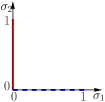
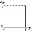
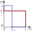
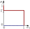
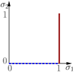
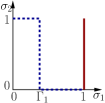
Figure 5: Plot of best response curves, $\sigma_{1}^{*}(\sigma_{2})$ and $\sigma_{2}^{*}(\sigma_{1})$, for $(r_{i},r_{j})$ in different regions. In each of these figures, the solid red curve is $\sigma_{1}^{*}(\sigma_{2})$ and the dashed blue curve is $\sigma_{2}^{*}(\sigma_{1})$. 5 $(r_{i},r_{j})\in\mathcal{R}_{1}$, 5 $(r_{i},r_{j})\in\mathcal{R}_{5}$, 5 $(r_{i},r_{j})\in\mathcal{R}_{4}$, 5 $(r_{i},r_{j})\in\mathcal{R}_{2a}$, 5 $(r_{i},r_{j})\in\mathcal{R}_{2b}$, and 5 $(r_{i},r_{j})\in\mathcal{R}_{2c}$.

Remark: The condition imposed on $\nu_{1}$ and $C^{(1)}$ in the above lemma is only to avoid the less interesting boundary cases. Also, note that $\Gamma_{2}$ is a function of the reward $r_{i}$ to $\mathscr{F}_{1}$. For notational simplicity we do not show $r_{i}$ as an argument of $\Gamma_{2}$.

Similarly, for $\mathscr{F}_{2}$ we can define $\sigma_{2}^{*}(\sigma_{1})$ as the set of all best responses against the strategy $\sigma_{1}$ played by $\mathscr{F}_{1}$, and obtain a result analogous to that in Lemma 8, but with quantities corresponding to $\mathscr{F}_{1}$ replaced by that corresponding to $\mathscr{F}_{2}$, e.g., for instance, $\zeta^{(1)}$ replaced by $\zeta^{(2)}$, $\alpha^{(1)}$ by $\alpha^{(2)}$, $\Gamma_{2}$ by $\Gamma_{1}$ where

$$\Gamma_{1}=\frac{-\eta_{2}r_{j}-C^{(2)}}{\Big{(}-\eta_{2}r_{j}-C^{(2)}\Big{)}-\Big{(}E^{(2)}(r_{j})-D^{(2)}\Big{)}}.$$ (82)

Now, for any $(r_{i},r_{j})$ the points of intersection between the best response curves $\sigma_{1}^{*}(\sigma_{2})$ and $\sigma_{2}^{*}(\sigma_{1})$ constitutes the NE strategies of the game in Table 4. For instance, as shown in Fig. 5, when $(r_{i},r_{j})$ is such that $r_{i}<\zeta^{(1)}$ and $r_{j}<\zeta^{(2)}$ (i.e., $(r_{i},r_{j})\in\mathcal{R}_{1}$; see Fig. 6) then the only point of intersection is $(0,0)$ so that $(\textsf{c},\textsf{c})$ is the only NE strategy in this region. Similarly when $(r_{i},r_{j})\in\mathcal{R}_{5}$ then $(\textsf{s},\textsf{s})$ is the only NE strategy (see Fig. 5). An interesting case is when $(r_{i},r_{j})\in\mathcal{R}_{4}$ (see Fig. 5) where there are multiple NE strategies, namely, $(\textsf{s},\textsf{c})$, $(\textsf{c},\textsf{s})$ and the mixed strategy $(\Gamma_{1},\Gamma_{2})$ (which depends on the reward pair $(r_{i},r_{j})$; see remark following Lemma 8).

The region $\mathcal{R}_{2}$ is written as a union of three disjoint regions, $\mathcal{R}_{2a}$, $\mathcal{R}_{2b}$ and $\mathcal{R}_{2c}$. However, as shown in Fig. 5 to 5, the best response curves for $(r_{i},r_{j})$ in each of these sub-regions intersect at $(1,0)$. Hence $(\textsf{s},\textsf{c})$ is the NE strategy in the union region $\mathcal{R}_{2}$. Similarly, $(\textsf{c},\textsf{s})$ is the NE strategy in region $\mathcal{R}_{3}$ which is also composed of three sub-regions.

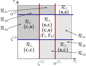
Figure 6: Illustration of the various regions along with the NE strategy corresponding to these regions.

$\mathcal{R}_{1}=\Big{\{}(r_{i},r_{j}):r_{i}<\zeta^{(1)},r_{j}<\zeta^{(2)}\Big{\}}$
$\mathcal{R}_{2}=\mathcal{R}_{2a}\cup\mathcal{R}_{2b}\cup\mathcal{R}_{2c}$ where
$\mathcal{R}_{2a}=\Big{\{}(r_{i},r_{j}):\zeta^{(1)}\leq r_{i}\leq\alpha^{(1)},r_{j}<\zeta^{(2)}\Big{\}}$
$\mathcal{R}_{2b}=\Big{\{}(r_{i},r_{j}):r_{i}>\alpha^{(1)},r_{j}<\zeta^{(2)}\Big{\}}$
$\mathcal{R}_{2c}=\Big{\{}(r_{i},r_{j}):r_{i}>\alpha^{(1)},\zeta^{(2)}\leq r_{j}\leq\alpha^{(2)}\Big{\}}$
$\mathcal{R}_{3}=\mathcal{R}_{3a}\cup\mathcal{R}_{3b}\cup\mathcal{R}_{3c}$ where
$\mathcal{R}_{3a}=\Big{\{}(r_{i},r_{j}):r_{i}<\zeta^{(1)},\zeta^{(2)}\leq r_{j}\leq\alpha^{(2)}\Big{\}}$
$\mathcal{R}_{3b}=\Big{\{}(r_{i},r_{j}):r_{i}<\zeta^{(1)},r_{j}>\alpha^{(2)}\Big{\}}$
$\mathcal{R}_{3c}=\Big{\{}(r_{i},r_{j}):\zeta^{(1)}\leq r_{i}\leq\alpha^{(1)},r_{j}>\alpha^{(2)}\Big{\}}$
$\mathcal{R}_{4}=\Big{\{}(r_{i},r_{j}):\zeta^{(1)}\leq r_{i}\leq\alpha^{(1)},\zeta^{(2)}\leq r_{j}\leq\alpha^{(2)}\Big{\}}$
$\mathcal{R}_{5}=\Big{\{}(r_{i},r_{j}):r_{i}>\alpha^{(1)},r_{j}>\alpha^{(2)}\Big{\}}$

TABLE 7: Formal definition of various regions depicted in Fig. 6.

We have thus identified a partition of the set $\{(r_{i},r_{j}):i,j\in[n]\}$ into five regions such that the set of NE strategies corresponding to each region are different. These regions along with the corresponding NE strategies are depicted in Fig. 6. A formal definition of the various regions is available in Table 7. Note that, these regions depend on the cost pair $\mathbf{C}=(C^{(1)},C^{(2)})$; for simplicity we have not shown this explicitly in Fig. 6 and in Table 7.

Appendix E Proof of Theorem 3

Theorem 3: Given a PO policy pair $(\overline{\pi}_{1}^{*},\overline{\pi}_{2}^{*})$, construct a strategy vector pair $\{({f}_{\ell}^{*},{g}_{\ell}^{*}):\ell\in\mathcal{L}\}$ as follows: $f_{\ell}^{*}(r_{i})=\overline{\pi}_{1}^{*}(r_{i},\ell)$ and ${g}_{\ell}^{*}(r_{j})=\overline{\pi}_{2}^{*}(\ell,r_{j})$ for all $i,j\in[n]$. Now, suppose for each $\ell$, $({f}_{\ell}^{*},{g}_{\ell}^{*})$ is a NE vector for $\mathcal{G}(\overline{\pi}_{1}^{*},\overline{\pi}_{2}^{*})$ such that,

$$\min\Big{\{}C^{(1)}_{\textsf{s},{g}_{\ell}^{*}}(r_{i}),C^{(1)}_{\textsf{c},{g}_{\ell}^{*}}\Big{\}} = G^{(1)}_{\overline{\pi}_{1}^{*},\overline{\pi}_{2}^{*}}(r_{i},\ell),\mbox{ and }$$

$$\min\Big{\{}C^{(2)}_{\textsf{s},f_{\ell}^{*}}(r_{j}),C^{(2)}_{\textsf{c},f_{\ell}^{*}}\Big{\}} = G^{(2)}_{\overline{\pi}_{1}^{*},\overline{\pi}_{2}^{*}}(\ell,r_{j}).$$

Then $(\overline{\pi}_{1}^{*},\overline{\pi}_{2}^{*})$ is a PO-NEPP.

Proof:

Given the policy pair $(\overline{\pi}_{1}^{*},\overline{\pi}_{2}^{*})$ as in the hypothesis, let $\overline{\pi}_{1}$ be any PO policy. We will show that $G^{(1)}_{\overline{\pi}_{1}^{*},\overline{\pi}_{2}^{*}}(r_{i},\ell)\leq G^{(1)}_{\overline{\pi}_{1},\overline{\pi}_{2}^{*}}(r_{i},\ell)$; the proof of, $G^{(1)}_{\overline{\pi}_{1}^{*},\overline{\pi}_{2}^{*}}(r_{i},\ell)\leq G^{(1)}_{\overline{\pi}_{1}^{*},\overline{\pi}_{2}}(r_{i},\ell)$ for any $\overline{\pi}_{2}$, is along similar lines.

Since $f_{\ell}^{*}=BR_{1}(g_{\ell}^{*})$, for the Bayesian game $\mathcal{G}(\overline{\pi}_{1}^{*},\overline{\pi}_{2}^{*})$, the expected cost incurred to $\mathscr{F}_{1}$ when its observation is $(r_{i},\ell)$ is $\min\Big{\{}C^{(1)}_{\textsf{s},g_{\ell}^{*}}(r_{i}),C^{(1)}_{\textsf{c},g_{\ell}^{*}}\Big{\}}$. Hence, using (57) we can write

$$G^{(1)}_{\overline{\pi}_{1}^{*},\overline{\pi}_{2}^{*}}(r_{i},\ell) \leq C^{(1)}_{\overline{\pi}_{1}(r_{i},\ell),g_{\ell}^{*}}(r_{i})$$

$$= \mathbb{E}_{\overline{\pi}_{1},\overline{\pi}_{2}^{*}}^{(r_{i},\ell)}\Big{[}g_{1}(X_{1},(A_{1,1},A_{2,1}))\Big{]}+\mathbb{E}_{\overline{\pi}_{1},\overline{\pi}_{2}^{*}}^{(r_{i},\ell)}\Big{[}G^{(1)}_{\overline{\pi}_{1}^{*},\overline{\pi}_{2}^{*}}(O_{1,2})\Big{]}.$$

Applying the above inequality $K$ times we obtain

$$G^{(1)}_{\overline{\pi}_{1}^{*},\overline{\pi}_{2}^{*}}(r_{i},\ell) \leq \sum_{k=1}^{K}\mathbb{E}_{\overline{\pi}_{1},\overline{\pi}_{2}^{*}}^{(r_{i},\ell)}\Big{[}g_{1}(X_{k},(A_{1,k},A_{2,k}))\Big{]}+\mathbb{E}_{\overline{\pi}_{1},\overline{\pi}_{2}^{*}}^{(r_{i},\ell)}\Big{[}G^{(1)}_{\overline{\pi}_{1}^{*},\overline{\pi}_{2}^{*}}(O_{1,K+1})\Big{]}.$$ (83)

Again, as in the proof of Theorem 1 Part-(b), we will assume that the PO policy pair $(\overline{\pi}_{1},\overline{\pi}_{2}^{*})$ is such that using this policy pair $\mathscr{F}_{1}$ will eventually terminate starting from any observation $o_{1}$, i.e.,

$$\lim_{K\rightarrow\infty}\mathbb{P}_{\overline{\pi}_{1},\overline{\pi}_{2}^{*}}^{o_{1}}(O_{1,K}=\textbf{\emph{t}}) = 1.$$ (84)

Hence we have

$$\lim_{K\rightarrow\infty}\mathbb{E}_{\overline{\pi}_{1},\overline{\pi}_{2}^{*}}^{(r_{i},\ell)}\Big{[}G^{(1)}_{\overline{\pi}_{1}^{*},\overline{\pi}_{2}^{*}}(O_{1,K+1})\Big{]} = G^{(1)}_{\overline{\pi}_{1}^{*},\overline{\pi}_{2}^{*}}(\textbf{\emph{t}})$$

$$= 0.$$

Using the above and recalling (48) while taking $\lim_{K\rightarrow\infty}$ in (83) we obtain $G^{(1)}_{\overline{\pi}_{1}^{*},\overline{\pi}_{2}^{*}}(r_{i},\ell)\leq G^{(1)}_{\overline{\pi}_{1},\overline{\pi}_{2}^{*}}(r_{i},\ell)$.

Finally, suppose the PO policy pair $(\overline{\pi}_{1},\overline{\pi}_{2}^{*})$ does not satisfy (84), then there is a positive probability that $\mathscr{F}_{1}$ will continue forever yielding $G^{(1)}_{\overline{\pi}_{1},\overline{\pi}_{2}^{*}}(r_{i},\ell)=\infty$. Thus for this case, $G^{(1)}_{\overline{\pi}_{1}^{*},\overline{\pi}_{2}^{*}}(r_{i},\ell)\leq G^{(1)}_{\overline{\pi}_{1},\overline{\pi}_{2}^{*}}(r_{i},\ell)$, trivially holds. ∎

Appendix F Proof of Lemma 5

Lemma 5: (1) Let $\Psi_{\ell},\Psi_{\ell}^{o}\in\mathcal{A}_{0}$ be two thresholds of $\mathscr{F}_{2}$ such that $\Psi_{\ell}<\Psi_{\ell}^{o}$, then the best response of $\mathscr{F}_{1}$ to these are ordered as, $BR_{1}(\Psi_{\ell})\geq BR_{1}(\Psi_{\ell}^{o})$. (2) Similarly, if $\Phi_{\ell},\Phi_{\ell}^{o}\in\mathcal{A}_{0}$ are two thresholds of $\mathscr{F}_{1}$ such that $\Phi_{\ell}<\Phi_{\ell}^{o}$ then $BR_{2}(\Phi_{\ell})\geq BR_{2}(\Phi_{\ell}^{o})$.

Proof:

For convenience, first let us recall the expressions of the costs $C_{\textsf{s},g_{\ell}}^{(1)}(r_{i})$ and $C_{\textsf{c},g_{\ell}}^{(1)}$ from (55) and (56) (since the given PO policy pair is $(\overline{\pi}_{1}^{*},\overline{\pi}_{2}^{*})$, these costs correspond to the Bayesian game $\mathcal{G}(\overline{\pi}_{1}^{*},\overline{\pi}_{2}^{*})$):

$$C_{\textsf{s},g_{\ell}}^{(1)}(r_{i}) = \widetilde{g}_{\ell}(-\eta_{1}r_{i})+(1-\widetilde{g}_{\ell})E^{(1)}(r_{i})$$ (85)

$$C_{\textsf{c},{g}_{\ell}}^{(1)} = \widetilde{g}_{\ell}\overline{C}^{(1)}_{\overline{\pi}_{1}^{*},\overline{\pi}_{2}^{*}}+(1-\widetilde{g}_{\ell})D^{(1)}.$$ (86)

Also, recall from (53) that the cost of continuing alone is less than the cost of continuing along with the competing forwarder, i.e.,

$${D}^{(1)}\leq\overline{C}^{(1)}_{\overline{\pi}_{1}^{*},\overline{\pi}_{2}^{*}}$$ (87)

We will only prove Part-(1); the proof of Part-(2) is similar. Let $g_{\ell}$ and $g_{\ell}^{o}$ be the threshold vectors of $\mathscr{F}_{2}$ whose corresponding thresholds are $\Psi_{\ell}$ and $\Psi_{\ell}^{o}$, respectively. Given that $\Psi_{\ell}<\Psi_{\ell}^{o}$, to prove $BR_{1}(\Psi_{\ell})\geq BR_{1}(\Psi_{\ell}^{o})$ it is sufficient to show that, for any $r_{i}$, $C_{\textsf{s},g_{\ell}}^{(1)}(r_{i})\leq C_{\textsf{c},g_{\ell}}^{(1)}$ implies $C_{\textsf{s},g_{\ell}^{o}}^{(1)}(r_{i})\leq C_{\textsf{c},g_{\ell}^{o}}^{(1)}$.

Let us begin with an $r_{i}$ such that $C_{\textsf{s},g_{\ell}}^{(1)}(r_{i})\leq C_{\textsf{c},g_{\ell}}^{(1)}$, or alternatively, (recall (85) and (86)) $r_{i}$ is such that,

$$\widetilde{g}_{\ell}(-\eta_{1}r_{i})+(1-\widetilde{g}_{\ell})E^{(1)}(r_{i}) \leq \widetilde{g}_{\ell}\overline{C}^{(1)}_{\overline{\pi}_{1}^{*},\overline{\pi}_{2}^{*}}+(1-\widetilde{g}_{\ell})D^{(1)}.$$

Substituting $E^{(1)}(r_{i})=\nu_{1}(-\eta_{1}r_{i})+\nu_{2}D^{(1)}$ in the above expression, and then simplifying we obtain,

$$-\eta_{1}r_{i} \leq \frac{\widetilde{g}_{\ell}\overline{C}^{(1)}_{\overline{\pi}_{1}^{*},\overline{\pi}_{2}^{*}}+(1-\widetilde{g}_{\ell})\nu_{1}D^{(1)}}{\widetilde{g}_{\ell}+(1-\widetilde{g}_{\ell})\nu_{1}}$$

Thus $-\eta_{1}r_{i}$, being less than the convex combination of the costs $\overline{C}^{(1)}_{\overline{\pi}_{1}^{*},\overline{\pi}_{2}^{*}}$ and $D^{(1)}$, is less than both of these. Further since ${D}^{(1)}\leq\overline{C}^{(1)}_{\overline{\pi}_{1}^{*},\overline{\pi}_{2}^{*}}$, there are only two cases which are possible: $-\eta_{1}r_{i}<D^{(1)}\leq\overline{C}^{(1)}_{\overline{\pi}_{1}^{*},\overline{\pi}_{2}^{*}}$, and $D^{(1)}\leq-\eta_{1}r_{i}\leq\overline{C}^{(1)}_{\overline{\pi}_{1}^{*},\overline{\pi}_{2}^{*}}$. We will consider these two cases separately below.

Case-1: Suppose $-\eta_{1}r_{i}<D^{(1)}\leq\overline{C}^{(1)}_{\overline{\pi}_{1}^{*},\overline{\pi}_{2}^{*}}$, then

$$E^{(1)}(r_{i}) = \nu_{1}(-\eta_{1}r_{i})+\nu_{2}D^{(1)}$$

$$\leq D^{(1)}.$$

Using the above two inequalities in the expression of $C_{\textsf{s},g_{\ell}^{o}}^{(1)}(r_{i})$, and then comparing with $C_{\textsf{c},g_{\ell}^{o}}^{(1)}$ we obtain $C_{\textsf{s},g_{\ell}^{o}}^{(1)}(r_{i})\leq C_{\textsf{c},g_{\ell}^{o}}^{(1)}$.

Case-2: Suppose $D^{(1)}\leq-\eta_{1}r_{i}\leq\overline{C}^{(1)}_{\overline{\pi}_{1}^{*},\overline{\pi}_{2}^{*}}$. Then we have $E^{(1)}(r_{i})\geq D^{(1)}$. Define $\kappa(p)$ for $p\in[0,1]$ as,

$$\kappa(p) = p\Big{(}-\eta_{1}r_{i}-E^{(1)}(r_{i})-\overline{C}^{(1)}_{\overline{\pi}_{1}^{*},\overline{\pi}_{2}^{*}}+D^{(1)}\Big{)}+\Big{(}E^{(1)}(r_{i})-D^{(1)}\Big{)}.$$ (88)

Since $-\eta_{1}r_{i}\leq\overline{C}^{(1)}_{\overline{\pi}_{1}^{*},\overline{\pi}_{2}^{*}}$ and $E^{(1)}(r_{i})\geq D^{(1)}$ we have, $\kappa(p)$ is decreasing in $p$. Hence we can write $\kappa(\widetilde{g}_{\ell}^{o})\leq\kappa(\widetilde{g}_{\ell})$ because, with $\Psi_{\ell}<\Psi_{\ell}^{o}$ we have,

$$\widetilde{g}_{\ell}=\sum_{j=1}^{\Psi_{\ell}}p^{(2)}_{j|\ell}\leq\sum_{j=1}^{\Psi_{\ell}^{o}}p^{(2)}_{j|\ell}=\widetilde{g}_{\ell}^{o}.$$ (89)

Finally, rearranging the terms in (88) one can obtain,

$$C_{\textsf{s},g_{\ell}^{o}}^{(1)}(r_{i})-C_{\textsf{c},g_{\ell}^{o}}^{(1)} = \kappa(\widetilde{g}_{\ell}^{o})$$

$$\leq \kappa(\widetilde{g}_{\ell})$$

$$= C_{\textsf{s},g_{\ell}}^{(1)}(r_{i})-C_{\textsf{c},g_{\ell}}^{(1)}$$

$$\overset{*}{\leq} 0,$$

where $*$ is because we started with an $r_{i}$ such that, $C_{\textsf{s},g_{\ell}}^{(1)}(r_{i})\leq C_{\textsf{c},g_{\ell}}^{(1)}$. ∎

Appendix G Obtaining Cooperative Optimal Policy Pair

We will first prove Lemma 6.

Lemma 6: The policy pair $(\pi_{1}^{\gamma},\pi_{2}^{\gamma})$ is Pareto optimal, i.e., for any other policy $(\pi_{1},\pi_{2})$,

• if $C^{(1)}_{\pi_{1},\pi_{2}}<C^{(1)}_{\pi_{1}^{\gamma},\pi_{2}^{\gamma}}$ then $C^{(2)}_{\pi_{1}^{\gamma},\pi_{2}^{\gamma}}<C^{(2)}_{\pi_{1},\pi_{2}}$, and

• if $C^{(2)}_{\pi_{1},\pi_{2}}<C^{(2)}_{\pi_{1}^{\gamma},\pi_{2}^{\gamma}}$ then $C^{(1)}_{\pi_{1}^{\gamma},\pi_{2}^{\gamma}}<C^{(1)}_{\pi_{1},\pi_{2}}$.

Proof:

We will prove Part-(1); the proof of Part-(2) is similar. Since $(\pi_{1}^{\gamma},\pi_{2}^{\gamma})$ is optimal for the problem in (60) we can write, for any policy pair $(\pi_{1},\pi_{2})$,

$$\gamma C^{(1)}_{\pi_{1}^{\gamma},\pi_{2}^{\gamma}}+(1-\gamma)C^{(2)}_{\pi_{1}^{\gamma},\pi_{2}^{\gamma}} \leq \gamma C^{(1)}_{\pi_{1},\pi_{2}}+(1-\gamma)C^{(2)}_{\pi_{1},\pi_{2}},$$

rewriting which we obtain

$$C^{(2)}_{\pi_{1}^{\gamma},\pi_{2}^{\gamma}} \leq \frac{\gamma}{1-\gamma}\Big{(}C^{(1)}_{\pi_{1},\pi_{2}}-C^{(1)}_{\pi_{1}^{\gamma},\pi_{2}^{\gamma}}\Big{)}+C^{(2)}_{\pi_{1},\pi_{2}}.$$

Now, if $C^{(1)}_{\pi_{1},\pi_{2}}<C^{(1)}_{\pi_{1}^{\gamma},\pi_{2}^{\gamma}}$ then from the above expression we have $C^{(2)}_{\pi_{1}^{\gamma},\pi_{2}^{\gamma}}<C^{(2)}_{\pi_{1},\pi_{2}}$. ∎

We now proceed to obtain $(C^{(1)}_{\pi_{1}^{\gamma},\pi_{2}^{\gamma}},C^{(2)}_{\pi_{1}^{\gamma},\pi_{2}^{\gamma}})$ by formulating the problem in (60) as an MDP. The state space, action space and the state transitions remain same as in Section V. However the one-step costs have to be appropriately modified to take into account the multiplier $\gamma$. Without writing down all the details we will proceed to the Bellman equation. The one-step costs will be evident from these.

For states of the form $(r_{i},\textbf{\emph{t}})$

$$J^{*}(r_{i},\textbf{\emph{t}}) = \min\Big{\{}-\gamma\eta_{1}r_{i},\gamma\tau+\sum_{i^{\prime}}p^{(1)}_{i^{\prime}}J^{*}(r_{i}^{\prime},\textbf{\emph{t}})\Big{\}}.$$ (90)

The first term in the $\min$ expression above corresponds to the cost of the joint-action $(\textsf{s},\textsf{s})$ or $(\textsf{s},\textsf{c})$ (since $\mathscr{F}_{2}$ has terminated, its action is irrelavent), and the second term is the expected cost of choosing $(\textsf{c},\textsf{s})$ (or $(\textsf{c},\textsf{c})$). Similarly, when the state is $(\textbf{\emph{t}},r_{j})$ we can write

$$J^{*}(\textbf{\emph{t}},r_{j}) = \min\Big{\{}-(1-\gamma)\eta_{2}r_{j},(1-\gamma)\tau+\sum_{j^{\prime}}p^{(2)}_{j^{\prime}}J^{*}(\textbf{\emph{t}},r_{j}^{\prime})\Big{\}}.$$ (91)

The more interesting case is when both forwarders are still competing, i.e., when the state is of the form $(r_{i},r_{j})$, where the optimality equation is

$$J^{*}(r_{i},r_{j})=\min\Big{\{}C_{\textsf{s},\textsf{c}},C_{\textsf{c},\textsf{s}},C_{\textsf{s},\textsf{s}},C_{\textsf{c},\textsf{c}}\Big{\}};$$ (92)

$C_{a_{1},a_{2}}$ is the expected cost (one-step $+$ future cost-to-go) of choosing the joint-action $(a_{1},a_{2})$. When the joint-action chosen is $(\textsf{s},\textsf{c})$, since $\mathscr{F}_{1}$ stops and $\mathscr{F}_{2}$ continues the one-step cost is $\Big{(}-\gamma\eta_{1}r_{i}+(1-\gamma)\tau\Big{)}$. The subsequent state is of the form $(\textbf{\emph{t}},r_{j^{\prime}})$ w.p. $p^{(2)}_{j^{\prime}}$. Hence the expression for $C_{\textsf{s},\textsf{c}}$ can be written as

$$C_{\textsf{s},\textsf{c}} = -\gamma\eta_{1}r_{i}+(1-\gamma)\tau+\sum_{j^{\prime}}p^{(2)}_{j^{\prime}}J^{*}(\textbf{\emph{t}},r_{j^{\prime}}).$$ (93)

Similarly $C_{\textsf{c},\textsf{s}}$ can be written as

$$C_{\textsf{c},\textsf{s}} = \gamma\tau-(1-\gamma)\eta_{2}r_{j}+\sum_{i^{\prime}}p^{(1)}_{i^{\prime}}J^{*}(r_{i^{\prime}},\textbf{\emph{t}}).$$ (94)

When both forwarders decide to stop then w.p. $\nu_{1}$, $\mathscr{F}_{1}$ gets the relay in which case the cost incurred is $C_{\textsf{s},\textsf{c}}$; otherwise, w.p. $\nu_{2}$, $\mathscr{F}_{2}$ get the relay and the cost incurred is $C_{\textsf{c},\textsf{s}}$. Hence

$$C_{\textsf{s},\textsf{s}} = \nu_{1}C_{\textsf{s},\textsf{c}}+\nu_{2}C_{\textsf{c},\textsf{s}}.$$ (95)

Finally, when both forwarders continue the one-step cost is simply $\Big{(}\gamma\tau+(1-\gamma)\tau\Big{)}=\tau$ and the subsequent state is still of the form $(r_{i^{\prime}},r_{j^{\prime}})$. Thus we can write

$$C_{\textsf{c},\textsf{c}} = \tau+\sum_{i^{\prime},j^{\prime}}p_{i^{\prime},j^{\prime}}J^{*}(r_{i^{\prime}},r_{j^{\prime}}).$$ (96)

From (95) note that $C_{\textsf{s},\textsf{s}}\geq\min\{C_{\textsf{s},\textsf{c}},C_{\textsf{c},\textsf{s}}\}$ which means that the joint-action $(\textsf{s},\textsf{s})$ can never be optimal. Thus, under cooperation the forwarders never compete for a relay; either $\mathscr{F}_{1}$ will choose the relay, or $\mathscr{F}_{2}$ will choose, or both continue. Expression (92) can therefore be simplified as

$$J^{*}(r_{i},r_{j})=\min\Big{\{}C_{\textsf{s},\textsf{c}},C_{\textsf{c},\textsf{s}},C_{\textsf{c},\textsf{c}}\Big{\}}.$$ (97)

One can perform value iteration to solve for $J^{*}$ in (90), (91) and (97). Given $J^{*}$ it is easy to obtain the optimal policy $(\pi_{1}^{\gamma},\pi_{2}^{\gamma})$ (simply choose the joint-action that minimizes the RHS of these expressions, breaking ties arbitrarily) and then the cost pair, $(C^{(1)}_{\pi_{1}^{\gamma},\pi_{2}^{\gamma}},C^{(2)}_{\pi_{1}^{\gamma},\pi_{2}^{\gamma}})$.

References

- [1] Y. Yao, S. Ngoga, D. Erman, and A. Popescu, “Competition-Based Channel Selection for Cognitive Radio Networks,” in IEEE Wireless Communications and Networking Conference, April 2012.
- [2] D. Niyato and E. Hossain, “Competitive Spectrum Sharing in Cognitive Radio Networks: A Dynamic Game Approach,” IEEE Transactions on Wireless Communications, vol. 7, no. 7, pp. 2651–2660, July 2008.
- [3] J. Kim, X. Lin, and N. Shroff, “Optimal Anycast Technique for Delay-Sensitive Energy-Constrained Asynchronous Sensor Networks,” IEEE/ACM Transactions on Networking, vol. 19, no. 2, pp. 484 –497, April 2011.
- [4] K. P. Naveen and A. Kumar, “Relay Selection for Geographical Forwarding in Sleep-Wake Cycling Wireless Sensor Networks,” IEEE Transactions on Mobile Computing, vol. 12, no. 3, pp. 475–488, 2013.
- [5] K. Akkaya and M. Younis, “A Survey on Routing Protocols for Wireless Sensor Networks,” Ad Hoc Networks, vol. 3, pp. 325–349, 2005.
- [6] M. Mauve, J. Widmer, and H. Hartenstein, “A Survey on Position-Based Routing in Mobile Ad-Hoc Networks,” IEEE Network, vol. 15, pp. 30–39, 2001.
- [7] E. Cinlar, Introduction to Stochastic Processes. Prentice-Hall, 1975.
- [8] A. Kumar, D. Manjunath, and J. Kuri, Wireless Networking. San Francisco, CA, USA: Morgan Kaufmann Publishers Inc., 2008.
- [9] D. Tse and P. Viswanath, Fundamentals of wireless communication. New York, NY, USA: Cambridge University Press, 2005.
- [10] K. P. Naveen and A. Kumar, “Relay Selection with Channel Probing in Sleep-Wake Cycling Wireless Sensor Networks,” ACM Transactions on Sensor Networks, vol. 11, no. 3, pp. 52:1–52:38, May 2015.
- [11] H. Takagi and L. Kleinrock, “Optimal Transmission Ranges for Randomly Distributed Packet Radio Terminals,” IEEE Transactions on Communications [legacy, pre - 1988], vol. 32, no. 3, pp. 246–257, 1984.
- [12] T. C. Hou and V. Li, “Transmission Range Control in Multihop Packet Radio Networks,” IEEE Transactions on Communications, vol. 34, no. 1, pp. 38–44, 1986.
- [13] R. Nelson and L. Kleinrock, “The Spatial Capacity of a Slotted ALOHA Multihop Packet Radio Network with Capture,” IEEE Transactions on Communications, vol. 32, no. 6, pp. 684–694, 1984.
- [14] M. Zorzi and R. R. Rao, “Geographic Random Forwarding (GeRaF) for Ad Hoc and Sensor Networks: Multihop Performance,” IEEE Transactions on Mobile Computing, vol. 2, pp. 337–348, 2003.
- [15] S. Liu, K. W. Fan, and P. Sinha, “CMAC: An Energy Efficient MAC Layer Protocol using Convergent Packet Forwarding for Wireless Sensor Networks,” in SECON ’07, 4th Annual IEEE Communications Society Conference on Sensor, Mesh and Ad Hoc Communications and Networks, June 2007.
- [16] P. Chaporkar and A. Proutiere, “Optimal Joint Probing and Transmission Strategy for Maximizing Throughput in Wireless Systems,” IEEE Journal on Selected Areas in Communications, vol. 26, no. 8, pp. 1546 –1555, October 2008.
- [17] N. B. Chang and M. Liu, “Optimal Channel Probing and Transmission Scheduling for Opportunistic Spectrum Access,” in MobiCom ’07: Proceedings of the 13th annual ACM international conference on Mobile computing and networking, 2007.
- [18] Freeman, “The secretary problem and its extensions: A review,” International Statistical Review, 1983.
- [19] R. N. Bradt, S. M. Johnson, and S. Karlin, “On Sequential Designs for Maximizing the Sum of Observations,” The Annals of Mathematical Statistics, vol. 27, no. 4, pp. 1060–1074, 12 1956.
- [20] D. P. Bertsekas, Dynamic Programming and Optimal Control, Vol. I. Athena Scientific, 2005.
- [21] S. Karlin, Stochastic Models and Optimal Policy for Selling an Asset, Studies in Applied Probability and Management Science / edited by Kenneth J. Arrow, Samuel Karlin, Herbert Scarf . Stanford University Press, Stanford, Calif, 1962.
- [22] I. David and O. Levi, “A New Algorithm for the Multi-item Exponentially Discounted Optimal Selection Problem,” European Journal of Operational Research, vol. 153, no. 3, pp. 782 – 789, 2004.
- [23] B. K. Kang, “Optimal Stopping Problem with Double Reservation Value Property,” European Journal of Operational Research, vol. 165, no. 3, pp. 765 – 785, 2005.
- [24] S. C. Albright, “A Bayesian Approach to a Generalized House Selling Problem,” Management Science, vol. 24, no. 4, pp. 432–440, 1977.
- [25] D. B. Rosenfield, R. D. Shapiro, and D. A. Butler, “Optimal Strategies for Selling an Asset,” Management Science, vol. 29, no. 9, pp. 1051–1061, 1983.
- [26] J.-I. Nakagami, “A Two-Person Noncooperative Game for Assets Selling Problem: Independent Case,” Computers and Mathematics with Applications, vol. 37, pp. 207 – 212, 1999.
- [27] N. Immorlica, R. Kleinberg, and M. Mahdian, “Secretary Problems with Competing Employers,” in Internet and Network Economics, ser. Lecture Notes in Computer Science, P. Spirakis, M. Mavronicolas, and S. Kontogiannis, Eds. Springer Berlin Heidelberg, 2006, vol. 4286, pp. 389–400.
- [28] D. Ramsey and K. Szajowski, “Bilateral Approach to the Secretary Problem,” in Advances in Dynamic Games, ser. Annals of the International Society of Dynamic Games, A. Nowak and K. Szajowski, Eds. Birkhäuser Boston, 2005, vol. 7, pp. 271–284.
- [29] J. Filar and K. Vrieze, Competitive Markov Decision Processes. New York, NY, USA: Springer-Verlag New York, Inc., 1996.
- [30] A. Fink, “Equilibrium in a Stochastic n-Person Game,” Hiroshima Mathematical Journal, vol. 28, no. 1, pp. 89–93, 1964.
- [31] F. Thuijsman and O. J. Vrieze, “Total Reward Stochastic Games and Sensitive Average Reward Strategies,” J. Optim. Theory Appl., vol. 98, no. 1, pp. 175–196, July 1998.
- [32] E. Altman, “Non Zero-Sum Stochastic Games in Admission, service and Routing Control in Queueing Systems,” Queueing Systems, vol. 23, pp. 259–279, 1996.
- [33] E. Altman, K. Avrachenkov, N. Bonneau, M. Debbah, R. El-Azouzi, and D. S. Menasche, “Constrained Cost-Coupled Stochastic Games with Independent State Processes,” Operations Research Letters, vol. 36, no. 2, pp. 160 – 164, 2008.
- [34] T. Raghavan and J. Filar, “Algorithms for Stochastic Games - A Survey,” Zeitschrift fur Operations Research, vol. 35, pp. 437–472, 1991.
- [35] L. S. Shapley, “Stochastic Games,” Proceedings of the National Academy of Sciences, vol. 39, no. 10, pp. 1095–1100, 1953.
- [36] A. Nowak and K. Szajowski, Advances in Dynamic Games: Applications to Economics, Finance, Optimization, and Stochastic Control, ser. Annals of the International Society of Dynamic Games. Birkhauser Boston, 2007.
- [37] E. Solan and R. V. Vohra, “Correlated Equilibrium in Quitting Games,” Mathematics of Operations Research, vol. 26, no. 3, pp. 601–610, 2001.
- [38] V. Pata, “Fixed Point Theorems and Applications,” 2014. [Online]. Available: www.mate.polimi.it/viste/pagina_personale/pp/121/FP.pdf
- [39] D. P. Bertsekas and J. N. Tsitsiklis, “An Analysis of Stochastic Shortest Path Problems,” Mathematics of Operations Research, vol. 16, pp. 580–595, 1991.
- [40] E. A. Hansen, D. S. Bernstein, and S. Zilberstein, “Dynamic Programming for Partially Observable Stochastic Games,” in Proceedings of the 19th national conference on Artifical intelligence, ser. AAAI’04. AAAI Press, 2004, pp. 709–715.
- [41] M. J. Osborne, An Introduction to Game Theory. Oxford University Press, USA, August 2003.
- [42] L. MacDermed, C. Isbell, and L. Weiss, “Markov Games of Incomplete Information for Multi-Agent Reinforcement Learning,” in AAAI Workshops, 2011.
- [43] Crossbow, “TelosB Mote Platform,” 2014. [Online]. Available: www.willow.co.uk/TelosB_Datasheet.pdf