Measurement of Hubble constant: Non-Gaussian Errors in HST Key Project Data

Abstract

Assuming the Central Limit Theorem, experimental uncertainties in any data set are expected to follow the Gaussian distribution with zero mean. We propose an elegant method based on Kolmogorov-Smirnov statistic to test the above; and apply it on the measurement of Hubble constant which determines the expansion rate of the Universe. The measurements were made using Hubble Space Telescope. Our analysis shows that the uncertainties in the above measurement are non-Gaussian.

1 Introduction

Uncertainties are inevitable outcome of any experiment and their role is to spread the measured value around the true value of the quantity being measured. If the experiment is free of systematic effects, one expects the uncertainties to be symmetrically distributed around zero. Further, if Central Limit Theorem holds, they should follow Normal distribution.The systematics, if present, have to be identified and removed separately. Treatment of the errors becomes more important in astronomy since sometimes it is hard to repeat or perform the experiments in controlled way unlike the laboratory experiments. In the present letter we propose an elegant way to use the Kolmogorov-Smirnov (hereafter KS) test to detect the non-Gaussian uncertainties in astrophysical data, and apply it in the measurements of Hubble Constant.

In standard Big-Bang cosmology, the universe expands according to the Hubble law, $v=H_{0}d$, where $v$ is the recessional velocity of a galaxy at a distance $d$, and $H_{0}$ is the Hubble constant, which determines the expansion rate at the current epoch. Since, the velocities are measured in km/s and distances in Mega parsec (Mpc), the common unit of $H_{0}$ is km/s/Mpc and till the mid-1990s, most of the measured values fall in the range $40\leq H_{0}\leq 100$ km/s/Mpc [1].

The value of Hubble constant is of fundamental importance for testing the framework of standard cosmology. It sets the age of the universe, size of the observable universe and defines the critical density of the universe, $\rho_{c}=3H_{0}^{2}/8\pi G$. Further, growth of structures in the universe also depend on the expansion rate, i.e., numerical value of $H_{0}$. The determination of many physical properties of galaxies and quasars (e.g., mass, luminosity, energy density) all require knowledge of the Hubble constant. Thus, determining the accurate value of $H_{0}$ is amongst the most important issues in cosmology.

More than eight decades have passed since Hubble (1929) initially published the Hubble law, however, pinning down the accurate value for the Hubble constant has been proved to be extremely challenging. The main difficulty lies in the measurement of accurate distances over cosmological scales.

Hubble Space Telescope (HST) was launched in 1990 to measure the Hubble constant accurately. A space observatory was required since atmospheric seeing does not allow to resolve the Cepheids and measure their period-luminosity relations to large distances. The high resolution imaging of HST extends this limit, and the effective search volume. It has several other advantages as well, e.g., observations can be scheduled independently of the phase of the Moon, the time of day, or weather, and there are no seeing variations.

One of the main key projects of HST was to measure the value of $H_{0}$ within 10% accuracy, based on Cepheid calibration of a number of secondary distance determination methods. Determining $H_{0}$ accurately requires the measurement of distances far enough away so that both the small- and large-scale motions of galaxies become small compared to the overall Hubble expansion. To extend the distance scale beyond the range of the Cepheids, a number of methods that provide relative distances were chosen. The HST Cepheid distances were used to provide an absolute distance scale for these otherwise independent methods, including the Type Ia supernovae (SNe Ia), the Tully-Fisher relation (TF), the fundamental plane (FP) for elliptical galaxies, surface brightness fluctuations(SBF), and Type II supernovae (SNe II). The final result of HST key project was published in [2] (hereafter F01). However, some issues related to the HST key project data have also been reported. [3] found statistically significant spatial variation in the value of $H_{0}$, indicating the directional anisotropy. The variation does not appear to be an artifact of the Galactic dust; and the overall structure in the map is not consistent with the distribution of dust in the Cosmic Background Explorer (COBE) map [4]. Using techniques based on extreme value theory [5], [6] have reported that the errors in HST key project data are non-Gaussian.

Our main task in this paper is to determine whether or not, the measurement errors in the HST key project data are Gaussian in nature?

2 HST Key Project compilation

It is natural for secondary distance indicators to be affected by their own systematic uncertainties. In order to use Cepheid calibration to a secondary method, one has to choose number of calibrating galaxies for a given method initially such that the final statistical uncertainty on the zero point for that method remain constrained to 5%. Prior to HST, number of such calibrating galaxies were very small, e.g., only five for Tully-Fisher relation, none for SNe Ia, one for surface brightness fluctuations, and none for Fundamental plane relation.

For the calibration of secondary methods of Key Project, Cepheid distances of 18 new galaxies were obtained, HST data for eight other galaxies were reanalyzed; and these distances were combined with the five other nearby galaxies. Thus a total of 31 calibrating galaxies were available to serve the purpose as shown in Table 2 of F01. The maximum distance of calibrating galaxies for each secondary method in pre-HST & post-HST era is shown in Table 1. It is clear from Table 1 that the distance to the farthest calibrating galaxy prior to HST is 3.7 Mpc, while in the post-HST era it is more than 20 Mpc. These galaxies were observed in the active star forming regions of sky, but low in apparent dust extinction. Observations carried in two different wavelength bands to be able to determine the magnitude of extinction. Also, High Surface Brightness regions were avoided in order to minimize the source confusion or crowding.

Table 1: Numbers of Cepheid Calibrators for Secondary Methods.

Secondary Method	$N(pre-HST)$	Max.dist	$N(post-HST)$	Max dist.
Type Ia Supernovae	0	n/a	06	22.4 Mpc
Tully-Fisher relation	5	3.70 Mpc	21	21.5 Mpc
Surface brightness flactuation	1	0.78 Mpc	06	19.0 Mpc
Fundamental Plane	0	n/a	03	22.4 Mpc
Type II Supernovae	1	0.05 Mpc	04	9.75 Mpc

Two different softwares (DoPHOT and ALLFRAME) were used by two different group of researchers; and they compared their results only at the end of data reduction phase. This double blind approach minimizes the systematic uncertainties in this phase.

The final HST Key Project data set consists of 78 data points of five varieties of secondary distance indicators(see Table 2). Out of which, 36 SNe Ia and 21 Tully-Fisher galaxy clusters and groups are listed in Table 6 and 7 of F01 respectively. 11 galaxy clusters containing Fundamental Plane for 224 early type galaxies and six galaxy clusters with SBF measurements are listed in Table 9 and 10 of F01 respectively. Except the Fundamental Plane method, the value of Hubble constant obtained from different methods vary slightly. Four type II SNe, which are listed in Table 11 of F01 are excluded from our analysis, since SNe II are non-standard candles. Instead we have chosen two data points from [7]. The complete data set is available in [3]. In all the cases, recessional velocities have been corrected to the Cosmic Microwave Background (CMB) Radiation frame and thus all the $H_{0}$ values belong to CMB frame. F01 find the value of $H_{0}$=72$\pm 3_{r}$$\pm 7_{s}$ km/s/Mpc. Table 2 shows the value and uncertainties(both random and systematics) obtained for each secondary distance indicator (SNe Ia, TF, SBF, FP & SNe II ).

Table 2: Uncertainties in $H_{0}$ for Secondary Methods

Secondary Method	No.of data points	Value of $H_{0}$	Uncertainties
Type Ia Supernovae	36	71	$\pm 2_{r}$$\pm 6_{s}$
Tully-Fisher relation	21	71	$\pm 3_{r}$$\pm 7_{s}$
Surface brightness flactuation	06	70	$\pm 5_{r}$$\pm 6_{s}$
Fundamental Plane	11	82	$\pm 6_{r}$$\pm 9_{s}$
Type II Supernovae†	04	72	$\pm 9_{r}$$\pm 7_{s}$

^† Excluded from our analysis , Instead we have chosen two data points for Tully-Fisher relation from [7]

3 Methodology: The $\chi$ Statistic and KS Test

Central Limit Theorem: Central Limit Theorem (hereafter CLT) is a fundamental theorem of statistics; and one can hardly overstate its importance. To explain the classical CLT [8], consider a sequence $\{X_{k}\}$ with $k=1,2,\ldots,n$ of mutually independent random variables with a common distribution. Suppose that $\mu$ and $\sigma^{2}$ are the mean and variance of the common distribution; and let $S_{n}:=\{X_{1}+X_{2}+\ldots+X_{n}\}/n$ be the mean of the sequence. According to the classical CLT, $\sqrt{n}(S_{n}-\mu)$ approximates the normal distribution with zero mean and $\sigma^{2}$ variance, i.e., N(0, $\sigma^{2}$). CLT is applicable if the random variables have finite mean and finite variance. For instance, if the sequence $\{X_{k}\}$ is drawn from the Cauchy distribution, the variance is not finite and hence CLT fails to hold. The classical version of CLT is also known as the Lindeberg-Levy CLT; however, some variants are also available. The Lyapunov CLT, for instance, does not require the random variables to be identically distributed.

With the technological advancement the precision of the observation has increased enormously. Consequently, the size of the error bars has reduced drastically, hence, we expect small errors (finite in size, hence finite variance). A considerably suitable combination of above mentioned fact with emergence of sofisticated statistical techniques of data analysis ensures the viability of CLT in astronomical observations.

$\chi$ Statistic: Consider the measurement of $H_{0}$ with true value $H_{0}^{true}$. The observed value $H_{0i}^{obs}$ in the $i^{th}$ measurement can be expressed as:

$$H_{0i}^{obs}=H_{0}^{true}\pm\sigma_{i};$$ (3.1)

where $\sigma_{i}$ stands for error in the $i{th}$ measurement. In the absence of systematic effects we expect the average of the errors to be zero, i.e., $\overline{\sigma}_{i}=0$. One can use appropriate statistical techniques, such as maximum likelihood, to obtain the best-fit value from the data. In this case the best-fit value will be same as the true value, i.e., ${H_{0}}^{bf}=H_{0}^{true}$. According to CLT, we also expect the errors to follow the Gaussian distribution. If we define:

$$\chi_{i}=\frac{H_{0i}^{obs}-H_{0}^{true}}{\sigma_{i}};$$ (3.2)

then, one expects $\chi_{i}$ to follow the standard normal, i.e., Gaussian distribution with zero mean and unit standard deviation. However, there could be systematic errors involved in the measurement, which would shift the best-fit value away from the true value; and thus $\chi_{i}$ defined in Eq. 3.2 would be biased. If systematic error in the measurement is $\epsilon$, Eq. 3.1 is modified to

$$H_{0i}^{obs}=H_{0}^{true}\pm\sigma_{i}+\epsilon\,.$$ (3.3)

So, the true value in Eq. 3.2 should be replaced with the best-fit value, ${H}_{0}^{bf}$. The equation takes the form

$$\chi_{i}=\frac{H_{0i}^{obs}-{H}_{0}^{bf}}{\sigma_{i}}\,;$$ (3.4)

If all the measurements in the data are statistically uncorrelated then the random variable, $\chi_{i}$, defined in Eq. 3.4 should follow a standard normal distribution. The method can be easily generalized; one can define $\chi_{i}$ for any physical observable $Y$. If the observed value in the $i^{th}$ measurement is $Y_{i}$, with uncertainty $\sigma_{i}$, then:

$$\chi_{i}=\frac{Y_{i}-{Y}^{bf}}{\sigma_{i}}\,;$$ (3.5)

where $Y^{bf}$ is the best-fit value of $Y$.

The KS Test: Kolmogorov-Smirnov test is a standard tool to determine whether or not a given sample follows the Gaussian distribution [9]. It compares the cumulative distribution function

$$F(x)=\int_{-\infty}^{x}f(x)dx$$ (3.6)

with the corresponding experimental quantity

$$S(x)=\frac{Number\,of\,observations\,with\,x_{i}<x}{Total\,Number}$$ (3.7)

The test statistic is the maximum difference $k$ between the two functions:

$$k=sup\{F(x)-S(x)\}$$ (3.8)

Table 3: Best-fit value for $H_{0}$.

Best-fit	$\chi^{2}$	$\chi^{2}_{\rm per\,dof}$
72.0	194.1	2.6

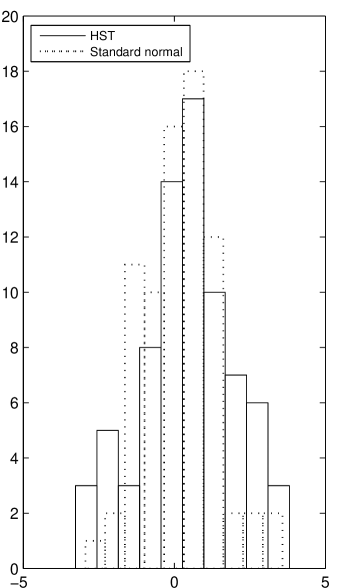
Figure 1: Histogram of $\chi_{i}$‘s is compared with that of standard normal distribution.

We set our null hypothesis as: “The errors in the HST key project data are Gaussian and hence $\chi_{i}$’s in Eq. 3.4 follow standard normal distribution". We apply KS test to calculate the test statistic and the p-value (the probability of obtaining the observed sample when the null hypothesis is actually true).

For this, we use Matlab function kstest[h,p,k,cv]; where $`k^{\prime}$ is the maximum distance between the two distributions, and $cv$ is the critical value which is decided by the significance level ($\alpha$). Different values of $\alpha$, indicate different tolerance levels for false rejection of the null hypothesis. For instance, $\alpha=0.01$ means that we allow 1% of the times to reject the null hypothesis when it is actually true. $cv$ is the critical probability to obtain/generate the data set in question given the null hypothesis. A value $h=1$ is returned by the test if $p<cv$ and the null hypothesis is rejected. While for $p>cv$, $h$ remains $0$ and the null hypothesis is not rejected.

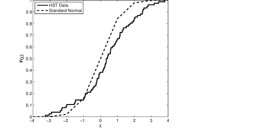
Figure 2: A comparison of cumulative distribution of $\chi_{i}$‘s with that of standard normal distribution.

4 Results

We first calculate the best-fit value of The Hubble constant, $H_{0}^{bf}$ by minimizing $\chi^{2}$.We obtain $H_{0}^{bf}=72$ km/s/Mpc, which is shown in Table 3. The value of $\chi^{2}$ is too large which suggests that the errors have been underestimated.

As a first check, we calculate $\chi_{i}$ for each data point and plot a histogram of the values in Fig 1. Mean and standard deviation of the $\chi_{i}$’s are $0.40$ and $1.55$ respectively. A histogram of 76 random numbers, generated using the Matlab function "randn", is also plotted in the same figure. It is clear from Fig 1 that the $\chi_{i}$‘s are spread more compared to the standard normal distribution and have thick tails.

Table 4: Results of KS-test.

$\alpha$	$cv$	$p$-value	$k$
0.01	0.1841	0.0048	0.1966
0.05	0.1534	0.0048	0.1966
0.10	0.1381	0.0048	0.1966

Results of KS test for $\chi_{i}$‘s are shown in Table 4. The $p$-value is only 0.48%, and is always smaller than $cv$. Thus the null hypothesis is always rejected. Fig. 2 shows the cumulative distribution of errors against that of Gaussian distribution. Difference between the two distributions is quite visible. Maximum vertical distance is $k=0.1966$.

5 Conclusion

We have presented a neat and simple method to detect the non-Gaussian errors in experimental data; and applied it on the HST Key Project data. Our analysis suggests the presence of non-Gaussian errors in the HST Key data. The possibility that the non-Gaussian part could be random with some other distribution seems unlikely in the light of CLT. The other possibility, that systematic effects are making the errors non-Gaussian seems plausible. The systematics could be attributed to any one or a combination of the following reasons: a) the unknown systematics of the secondary methods; b) zero-point of Cepheid P-L relation is not well determined; c) metallicity dependence of the zero-point of P-L relation; d) systematic effects arising in the data reduction techniques (in some cases, DoPHOT and ALLFRAME give different results); e) calibration of various instruments e.g., complicacy in charge transfer efficiency of WFPC2 etc. The detailed treatment of systematics and the method used, could find its profound impact on improving instrumentation of ongoing and future missions.

References

- [1] Tanvir, N. R., Shanks, T., Ferguson, H. C., Determination of the Hubble constant from observations of Cepheid variables in the galaxy M96, Nature 377,27 (1995).
- [2] Freedman, W. L., Madore, B. F., Gibson, B. K., Final Results from the Hubble Space Telescope Key Project to Measure the Hubble Constant, ApJ 553,47 (2001).
- [3] M. L. McClure, C. C. Dyer., Anisotropy in the Hubble constant as observed in the HST Extragalactic Distance Scale Key Project results, New Astronomy 12,7 (2007).
- [4] Schlegel, D. J., Finkbeiner, D. P., Davis, M., Maps of Dust IR Emission for Use in Estimation of Reddening and CMBR Foregrounds, ApJ 500,525. (1998).
- [5] Gupta Shashikant and Saini Tarun Deep., Direction Dependence in Supernovae Data, MNRAS 407,651 (2010).
- [6] Gupta Shashikant and Saini Tarun Deep., Non-Gaussianity in the HST Key Project data, MNRAS 415,2594 (2011).
- [7] Sakai, S., Mould, J. R., Hughes, S. M. G., et al., The Hubble Space Telescope Key Project on the Extragalactic Distance Scale XXIV: The Calibration of Tully-Fisher Relations and the Value of the Hubble Constant, ApJ 529,698. (2000).
- [8] Feller W., An Introduction to Probability Theory and its Applications, Wiley (2008).
- [9] Press, W. H.,The art of scientific computing, Cambridge University Press 12,7 (2007).