Macroscopic Time-Reversal Symmetry Breaking at Nonequilibrium Phase Transition

Abstract

We study the entropy production in a macroscopic nonequilibrium system that undergoes an order-disorder phase transition. Entropy production is a characteristic feature of nonequilibrium dynamics with broken detailed balance. It is found that the entropy production rate per particle vanishes in the disordered phase and becomes positive in the ordered phase following critical scaling laws. We derive the scaling relations for associated critical exponents. Our study reveals that a nonequilibrium ordered state is sustained at the expense of macroscopic time-reversal symmetry breaking with an extensive entropy production while a disordered state costs only a subextensive entropy production.

Detailed balance is the hallmark of the thermal equilibrium state. A system is said to obey detailed balance if the probability current along any microscopic trajectory in the phase space is balanced by that along the time-reversed one Gardiner (2010). Consequently, time-reversal symmetry is preserved in thermal equilibrium.

Thermodynamics of nonequilibrium systems, where detailed balance and time-reversal symmetry are broken with a positive entropy production, has been attracting a lot of interests Evans et al. (1993); Gallavotti and Cohen (1995); Jarzynski (1997); Sekimoto (1998); Lebowitz and Spohn (1999); Crooks (1999); Seifert (2005). Recent studies have been focused on microscopic systems with a few degrees of freedom where the effect of thermal fluctuations are strong. Under the framework of stochastic thermodynamics, various fluctuation theorems are discovered, which provide useful insights on the nature of nonequilibrium fluctuations. Theoretical works foster experimental studies of microscopic systems such as molecular motors, nano heat engines, biomolecules, and so on Wang et al. (2002); Carberry et al. (2004); Collin et al. (2005); Blickle and Bechinger (2011); Gomez-Solano et al. (2011); Lee et al. (2015).

Macroscopic systems pose an intriguing question on the level of irreversibility. Consider a many-particle system displaying an order-disorder phase transition whose microscopic dynamics does not obey detailed balance. Does the broken detailed balance result in time-reversal symmetry breaking at the macroscopic level? On the one hand, one may expect that entropy productions of each particle add up to a macroscopic amount irrespective of a macroscopic state. On the other hand, if the system is in a disordered phase so that all configurations are almost equally likely, then irreversibility may not show up on a macroscopic level producing only a subextensive amount of entropy. A system in an ordered state has a lower entropy than in a disordered state. Then, which phase produces more total entropy including the system entropy and the environmental entropy? These questions lead us to the study of the entropy production in a model system undergoing nonequilibrium phase transition.

In this paper, we investigate the emergence of macroscopic irreversibility out of microscopic dynamics with broken detailed balance. We find that the total entropy production changes its character from being subextensive to being extensive as the system undergoes an order-disorder phase transition. The entropy production rate per particle exhibits critical scaling laws as an order parameter does in ordinary critical phenomena, and scaling relations among critical exponents are derived. Although the results are derived in a specific model system, we argue that the scaling behaviors should be valid for general nonequilibrium systems.

As a nonequilibrium model, we adopt the particle system in two dimensions introduced in Ref. Sevilla et al. (2014). This model describes a flocking phenomenon of passive particles. In nature a flock of birds and a school of fish display a collective motion Vicsek and Zafeiris (2012). Such a phenomenon has been studied with microscopic models consisting of active self-propelled particles moving at a constant speed Vicsek et al. (1995); Grégoire and Chaté (2004). Flocking takes place when particles are subject to an interaction that favors alignment of individual velocities to the mean direction.

The model in Ref. Sevilla et al. (2014) is composed of passive particles in the thermal reservoir instead of active particles. It consists of $N$ Brownian particles of mass $m$ in a two-dimensional plane of size $L\times L$ embedded in a thermal reservoir at constant temperature $T$. The particle density is denoted by $\rho=N/L^{2}$. Let ${\bm{x}}_{i}=(x_{i1},x_{i2})$ and $\bm{v}_{i}=\frac{d{\bm{x}}_{i}}{dt}=(v_{i1},v_{i2})$ be the position and the velocity of a particle $i=1,\cdots,N$. We will represent a configuration of the whole system with a short-hand notation $\bm{Z}=(\bm{X},\bm{V})$ with $\bm{X}=\{{\bm{x}}_{1},{\bm{x}}_{2},\cdots,{\bm{x}}_{N}\}$ and $\bm{V}=\{{\bm{v}}_{1},{\bm{v}}_{2},\cdots,{\bm{v}}_{N}\}$. The equations of motion are given by

$$m\frac{d{\bm{v}}_{i}}{dt}={\bm{F}}_{i}(\bm{V})-\gamma{\bm{v}}_{i}+{\bm{\xi}}_{i}(t)$$ (1)

where $\gamma$ is the damping coefficient and ${\bm{\xi}}_{i}(t)=(\xi_{i1}(t),\xi_{i2}(t))$ is the thermal noise satisfying

$$\left\langle\xi_{ia}(t)\right\rangle =0$$ (2)

$$\left\langle\xi_{ia}(t)\xi_{jb}(t^{\prime})\right\rangle =2\gamma k_{B}T\delta_{ij}\delta_{ab}\delta(t-t^{\prime})$$

with the Boltzmann constant $k_{B}$, which will be set to unity hereafter. The velocity aligning force ${\bm{F}}_{i}(\bm{V})$ is taken to be

$${\bm{F}}_{i}(\bm{V})=\Gamma\hat{\bm{v}}_{i}\times(\bm{f}\times\hat{\bm{v}}_{i})=\Gamma\left(\bm{f}-(\bm{f}\cdot\hat{\bm{v}}_{i})\hat{\bm{v}}_{i}\right),$$ (3)

where $\Gamma$ is the interaction strength, $\hat{\bm{v}}_{i}={\bm{v}}_{i}/|{\bm{v}}_{i}|$ is the unit vector, and

$$\bm{f}=\frac{1}{N}\sum_{j=1}^{N}\hat{\bm{v}}_{j}\ .$$ (4)

The vector $\bm{f}$ points towards the average direction of the particles, and its magnitude $\Lambda=|\bm{f}|$ plays a role of the order parameter for the collective motion. Note that the force $\bm{F}_{i}$ is perpendicular to ${\bm{v}}_{i}$. It does not work on the particle but turns the direction of ${\bm{v}}_{i}$ toward $\bm{f}$. The interaction is infinite-ranged. A short-ranged version of the model was studied in Ref. Dossetti and Sevilla (2014).

Numerical study in Ref. Sevilla et al. (2014) found that the system undergoes a phase transition separating a disordered phase ($\Gamma<\Gamma_{c}$) and an ordered phase ($\Gamma>\Gamma_{c}$). Near $\Gamma=\Gamma_{c}$, the order parameter scales as $\langle\Lambda\rangle_{s}\sim(\Gamma-\Gamma_{c})^{\beta}$ and the susceptibility $\chi\equiv N(\langle\Lambda^{2}\rangle_{s}-\langle\Lambda\rangle_{s}^{2})$ scales as $\chi\sim|\Gamma-\Gamma_{c}|^{-\gamma}$, where $\langle\rangle_{s}$ denotes the steady-state ensemble average. The critical exponents are given by $\beta/\nu\simeq 0.491$ and $\gamma/\nu\simeq 1.02$, where $\nu\simeq 0.94$ is the correlation length exponent ($\xi\sim|\Gamma-\Gamma_{c}|^{-\nu}$) Sevilla et al. (2014). These exponents are compatible with those of the mean field XY model Kim et al. (2001); Sasa (2015). When the interaction is infinite-ranged, the correlation volume $\xi_{V}$ is more useful than the correlation length $\xi$. Since the model under consideration is embedded in the two-dimensional space, the correlation volume is given by $\xi_{V}=\xi^{2}$ and scales as $\xi_{V}\sim|\Gamma-\Gamma_{c}|^{-\bar{\nu}}$ with $\bar{\nu}=2\nu$.

The velocity-dependent force breaks the detailed balance and the time-reversal symmetry. We quantify the amount of the time-reversal symmetry breaking by the entropy production. Suppose that the system evolves along a stochastic trajectory $\mathcal{Z}[\tau]=\{(\bm{X}(t),\bm{V}(t))|0\leq t\leq\tau\}$ for a time interval $\tau$. Following stochastic thermodynamics Seifert (2005), the total entropy production $\Delta S_{\rm tot}[\mathcal{Z}[\tau]]$ along a given trajectory $\mathcal{Z}[\tau]$ is determined by the probability ratio of $\mathcal{Z}[\tau]$ against its time-reversed trajectory $\mathcal{Z}^{R}[\tau]=\{(\bm{X}(\tau-t),-\bm{V}(\tau-t))|0\leq t\leq\tau\}$ Seifert (2005); Spinney and Ford (2012); Lee et al. (2013); Ganguly and Chaudhuri (2013); Chaudhuri (2014); Kwon et al. (2015).

In our model, the total entropy production is decomposed into three terms as not

$$\Delta S_{\rm tot}[\mathcal{Z}]=\Delta S_{\rm sys}[\mathcal{Z}]-\frac{Q[\mathcal{Z}]}{T}+\Delta S_{\rm v}[\mathcal{Z}],$$ (5)

where $\Delta S_{\rm sys}$ is the change in the Shannon entropy of the system, the second term is the Clausius form for the entropy change of the heat bath with $Q$ being the heat absorbed by the system, and the last term $S_{\rm v}$ appears only in the presence of a velocity-dependent force Kwon et al. (2015) and is given by

$$\Delta S_{\rm v}[\mathcal{Z}]=\frac{m}{\gamma T}\sum_{i=1}^{N}\int_{0}^{\tau}dt\bm{F}_{i}(\bm{V}(t))\circ\frac{d{\bm{v}}_{i}(t)}{dt}.$$ (6)

In the steady state, the ensemble average of $\Delta S_{\rm sys}$ vanishes. The thermodynamic first law reads as $\Delta E=Q+W$ where $\Delta E$ is the change in the total energy $E=\sum_{i}\frac{1}{2}m{\bm{v}}_{i}^{2}$ and $W=\sum_{i}\int_{0}^{t}dt{\bm{v}}_{i}\cdot{\bm{F}}_{i}$ is the work done by the force. Since $W=0$, $Q=\Delta E$ and its steady state average vanishes. Thus, the entropy production rate per particle in the steady state is given by

$$s\equiv\frac{1}{N}\left\langle\frac{dS_{\rm tot}}{dt}\right\rangle_{s}=\frac{m}{\gamma T}\frac{1}{N}\sum_{i=1}^{N}\left\langle{\bm{F}}_{i}\circ\frac{d{\bm{v}}_{i}}{dt}\right\rangle_{s}.$$ (7)

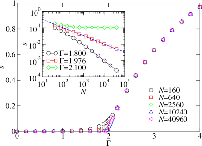
Figure 1: $s$ versus $\Gamma$ for several values of $N$. Inset shows the finite size scaling behaviors of $s$ when $\Gamma$ is below, equal to, and above $\Gamma_{c}=1.976$. The dotted (dashed) line has the slope $-1$ ($-1/2$).

We have performed numerical simulations. The equations of motion in (1) are integrated numerically by using the time-discretized ($\Delta t=0.01$) Heun algorithm Greiner et al. (1988). We took $m=\gamma=\rho=2T=1$ in all simulations. Figure 1 shows that $s$ displays a characteristic behavior signaling a continuous phase transition. As $N$ increases, $s\sim 1/N$ for $\Gamma<\Gamma_{c}$ while it converges to a finite value for $\Gamma>\Gamma_{c}$. We also measure the susceptibility of the entropy production that is defined as

$$\chi_{s}(\Gamma,N,\tau)=\frac{1}{\tau N}\left[\left\langle\Delta S_{\rm v}^{2}\right\rangle_{s}-\left\langle\Delta S_{\rm v}\right\rangle_{s}^{2}\right],$$ (8)

where $\Delta S_{\rm v}$ denotes the entropy production of $N$ particles in a time interval $\tau$. Figure 2 (a) shows the susceptibility measured at fixed $\tau=64$. It has a sharp peak at $\Gamma=\Gamma_{c}$, which also reminds us of a continuous phase transition. The threshold $\Gamma_{c}\simeq 1.976$ is close to the onset of the collective motion reported in Ref. Sevilla et al. (2014). We will show that the entropy production indeed exhibits the continuous phase transition and that the phase transition is triggered by the onset of the collection motion.

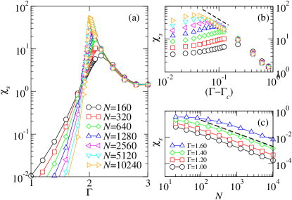
Figure 2: (a) Susceptibility $\chi_{s}$ as a function of $\Gamma$. (b) $\chi_{s}$ versus $(\Gamma-\Gamma_{c})$ in the log-log scale. The dashed line has the slope $-1$. (c) $\chi_{s}$ versus $N$ for $\Gamma<\Gamma_{c}$. The dashed line has the slope $-1$.

The entropy production can be related to the order parameter $\Lambda$ for the collective motion. Using the equations of motion for $d{\bm{v}}_{i}/dt$, the entropy production in (6) is written as not

$$\Delta S_{\rm v}= \sum_{i=1}^{N}\int_{0}^{\tau}dt\left[\frac{1}{\gamma T}|{\bm{F}}_{i}|^{2}+\frac{1}{m}\bm{\nabla}_{{\bm{v}}_{i}}\cdot{\bm{F}}_{i}\right]\$$ (9)

$$+\sum_{i=1}^{N}\frac{1}{\gamma T}\int_{0}^{\tau}{\bm{F}}_{i}\cdot d\bm{W}_{i}(t),$$

where $\bm{\nabla}_{{\bm{v}}_{i}}$ denotes the gradient operator with respective to ${\bm{v}}_{i}$ and $d\bm{W}_{i}(t)=\int_{t}^{t+dt}dt^{\prime}{\bm{\xi}}_{i}(t^{\prime})$. The last term contributes neither to the ensemble average nor to the susceptibility because it is of the order of $\mathcal{O}(\tau^{1/2})$ with zero mean while the others scale linearly with $\tau$. Hence, it will be ignored. We then introduce the polar coordinate so that the velocity vector is written as ${\bm{v}}_{i}=(v_{i}\cos\theta_{i},v_{i}\sin\theta_{i})$. The relation (4) for the vector $\bm{f}=(\Lambda\cos\psi,\Lambda\sin\psi)$ is written as

$$\Lambda e^{i\psi}=\frac{1}{N}\sum_{j=1}^{N}e^{i\theta_{j}}\ .$$ (10)

By using (3) and (10), we can show that not

$$\Delta S_{\rm v}=\sum_{i=1}^{N}\int_{0}^{\tau}dt\left[A_{i}-B_{i}+C_{i}\right]+\mathcal{O}(\tau^{1/2}),$$ (11)

where $A_{i}=\frac{\Gamma^{2}\Lambda^{2}}{\gamma T}\sin^{2}(\psi-\theta_{i})$, $B_{i}=\frac{\Gamma\Lambda}{mv_{i}}\cos(\psi-\theta_{i})$, and $C_{i}=\frac{\Gamma}{Nmv_{i}}$.

The expression in (11) gives a hint on the scaling behavior of the entropy production. The macroscopic variables $\Lambda$ and $\psi$ fluctuate much slower than the microscopic variables $v_{i}$’s and $\theta_{i}$’s. Thus, in taking the ensemble-average of (11), we can use the adiabatic approximation Sasa (2015) to replace $\Lambda^{2}$ and $\Lambda$ with their ensemble averaged values. Power counting combined with the adiabatic approximation leads to the conclusion that the entropy production rate per particle scales as $s\sim{\langle\Lambda^{2}\rangle_{s}}\sim\langle\Lambda\rangle_{s}^{2}$ (from $A_{i}$ and $B_{i}$) with the $\mathcal{O}(N^{-1})$ correction (from $C_{i}$). Therefore, we expect that the entropy production rate per particle exhibits a critical power law scaling

$$s\sim(\Gamma-\Gamma_{c})^{\beta_{e}}$$ (12)

with the critical exponent

$$\beta_{e}=2\beta$$ (13)

for $\Gamma>\Gamma_{c}$ and $s\sim 1/N$ for $\Gamma<\Gamma_{c}$. When $N$ is finite, following the standard finite-size-scaling (FSS) ansatz, we expect that

$$s=N^{-\beta_{e}/\bar{\nu}}\Phi\left((\Gamma-\Gamma_{c})N^{1/\bar{\nu}}\right).$$ (14)

The scaling function $\Phi(x)$ has the limiting behaviors $\Phi(x)\stackrel{{\scriptstyle x\gg 1}}{{\longrightarrow}}x^{\beta_{e}}$ ensuring (12) and $\Phi(x)\stackrel{{\scriptstyle x\ll-1}}{{\longrightarrow}}|x|^{\beta_{e}-\bar{\nu}}$ guaranteeing the $N^{-1}$ scaling in the disordered phase.

The numerical data in Fig. 1 are analyzed according to the FSS form with the mean field critical exponents $\beta_{e}=1$ and $\bar{\nu}=2$. As shown in Fig. 3, the data collapse and the limiting behaviors of the scaling function confirm the scaling relation in (13) and the FSS form of (14).

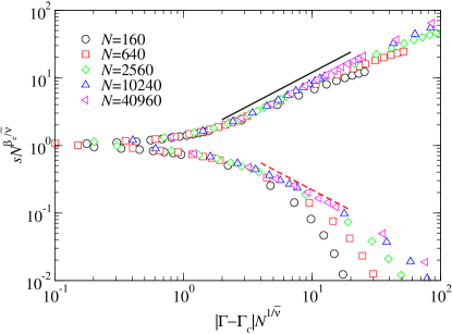
Figure 3: (Color online) Scaling plot of $sN^{\beta_{e}/\bar{\nu}}$ versus $|\Gamma-\Gamma_{c}|N^{1/\bar{\nu}}$ according to (14). The solid (dashed) line has slope $1~{}(-1)$.

The total entropy production $\Delta S_{\rm v}$ is given by the spatial and temporal sum of the fluctuating local entropy production rates. We can derive the scaling form for the susceptibility $\chi_{s}$ in the following way: Near the critical point, the correlation volume and time diverge as $\xi_{V}\sim|\Gamma-\Gamma_{c}|^{-\bar{\nu}}$ and $\xi_{t}\sim|\Gamma-\Gamma_{c}|^{-\nu_{t}}$, respectively. When $N\gg\xi_{V}$ and $\tau\gg\xi_{t}$ in the ordered phase ($\Gamma>\Gamma_{c}$), the total entropy production $\Delta S_{\rm v}$ is the sum of the contributions from $M=\tau N/(\xi_{t}\xi_{V})$ space-time blocks. All the blocks are independent because they are beyond the correlation volume and time. Therefore, the susceptibility should scale as $\chi_{s}\sim\frac{1}{\tau N}\times M\times(\xi_{t}\xi_{V}s)^{2}\sim\xi_{t}\xi_{V}s^{2}$, which leads to the scaling form

$$\chi_{s}\sim(\Gamma-\Gamma_{c})^{-\gamma_{e}}$$ (15)

with the susceptibility exponent

$$\gamma_{e}=\nu_{t}+\bar{\nu}-2\beta_{e}.$$ (16)

This is the hyperscaling relation extended to the systems with anisotropic scaling Hong et al. (2007); Henkel and Schollwöck (2001). At the critical point, the finite-size effect dominates so that

$$\chi_{s}(\Gamma_{c},N,\tau)\sim\left\{\begin{array}[]{ccc}\tau^{\gamma_{e}/\nu_{t}}&,&\tau\ll N^{\bar{z}}\\[5.69054pt] N^{\gamma_{e}/\bar{\nu}}&,&\tau\gg N^{\bar{z}}\end{array}\right.$$ (17)

with $\bar{z}=\nu_{t}/\bar{\nu}$. In the disordered phase, the entropy production rate per particle vanishes as $s\sim 1/N$, so does the susceptibility $\chi_{s}\sim 1/N$.

The numerical data support the scaling theory. Figure 2 (b) shows the susceptibility follows the power law of (15) with $\gamma_{e}=1$. This exponent value satisfies the hyperscaling relation in (16) with $\nu_{t}=1$, $\bar{\nu}=2$, and $\beta_{e}=1$. The $1/N$ scaling inside the disordered phase is also checked in Figure 2 (c). The FSS behavior at the critical point $\Gamma=\Gamma_{c}$ is examined in Fig. 4. At a given $N$, $\chi_{s}(\Gamma_{c},N,\tau)$ increases algebraically with $\tau$ and saturates to a limiting value (see Fig. 4(a)). The scaling plot in Fig. 4(b) confirms the scaling behavior of (17) for $\tau\ll N^{\bar{z}}$ and $\tau\gg N^{\bar{z}}$.

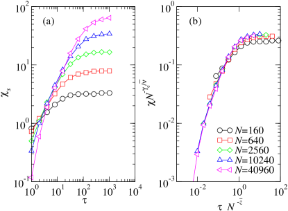
Figure 4: (Color online) (a) $\chi_{s}(\Gamma_{c},N,\tau)$ versus $\tau$ at several values of $N$. (b) Scaling plot of $\chi_{s}(\Gamma_{c},N,\tau)N^{-\gamma_{e}/\bar{\nu}}$ versus $\tau N^{-\bar{z}}$.

We have shown that the broken detailed balance leads to the macroscopic entropy production only in the ordered phase using the analytic scaling theory and the numerical simulations. The entropy production per particle per unit time $s$ is positive but vanishes as $1/N$ in the disordered phase, while it is finite in the ordered phase following the power law (see (12)). The susceptibility $\chi_{s}$ vanishes in the disordered phase and follows the power law (see (15)) in the ordered phase. The critical exponents satisfy the scaling relations in (13) and (16).

The quadratic relation $s\sim\langle\Lambda\rangle_{s}^{2}$ is crucial in deriving the scaling theory. This relation is derived in a model system that has a mean field nature. We argue that the scaling behaviors are universal in general thermal systems undergoing a nonequilibrium phase transition between a disordered phase and an ordered phase. Collective motions in the ordered phase are characterized by the thermodynamic currents $J_{i}$ of e.g., energy and particle. The currents are small near the critical point. Thus, following the linear irreversible thermodynamics of Onsager Onsager (1931), one can assume that $J_{i}=\sum_{j}L_{ij}X_{j}$ where $X_{j}$’s are the thermodynamic forces and $L_{ij}$’s are the Onsager coefficients. The entropy production rate is then given by $dS/dt=\sum_{i}X_{i}J_{i}=\sum_{i,j}L^{-1}_{ij}J_{i}J_{j}\propto J^{2}$, which supports the validity of the quadratic relation between the entropy production rate and the current density. In stochastic thermodynamics, the total entropy production rate is written as the configuration space average of the probability current density squared Seifert (2005), which also supports the relation. It would be interesting to investigate the scaling relations in (13) and (16) in systems with a short-ranged interaction.

The result that the ordered phase costs more environmental entropy production may be understood in the framework of the thermodynamic second law. Suppose that one changes a coupling constant of a system so that it relaxes from a disordered phase to an ordered phase in a characteristic relaxation time $t_{\rm relax}$. During the process, the system entropy decreases at the rate $dS_{\rm sys}/dt\sim\Delta S_{\rm sys}/t_{\rm relax}=(S_{\rm sys}({\rm ordered})-S_{\rm sys}({\rm disordered}))/t_{\rm relax}<0$. The thermodynamic second law requires that the entropy production rate should be nonnegative at any moment. Therefore, during the relaxation process, the environmental entropy production rate should satisfy $d{S}_{\rm env}/dt\geq-dS_{\rm sys}/dt\sim|\Delta S_{\rm sys}|/t_{\rm relax}$, which gives a lower bound for the environmental entropy production rate. It should be investigated further whether the inequality is working in the steady state. We leave it for future work.

This work was supported by the Basic Science Research Program through the NRF Grant No. 2013R1A2A2A05006776.

Appendix A Appendix: Total entropy production

It is straightforward to decide whether a deterministic dynamics is reversible or not. Suppose that a system evolves from a configuration $Z(0)=(X(0),V(0))$ to $Z(\tau)=(X(\tau),V(\tau))$ along a trajectory $\mathcal{Z}[\tau]=\{Z(t)|0\leq t\leq\tau\}$. If one flips the velocity in the final configuration and takes the resulting configuration $(X(\tau),-V(\tau))$ as an initial state, then the reversible dynamics lets the system follow the time-reversed trajectory $\mathcal{Z}^{R}[\tau]=\{Z^{R}(t)|0\leq t\leq\tau\}$ with $Z^{R}(t)\equiv(X(\tau-t),-V(\tau-t))$.

Generalizing this idea to stochastic systems, one can define the irreversibility or the entropy production by comparing the probability of trajectories $\mathcal{Z}[\tau]$ and $\mathcal{Z}^{R}[\tau]$. The probability distribution function (PDF) of a given trajectory $\mathcal{Z}[\tau]$ is given by $P[\mathcal{Z}[\tau]]=\Pi\left[\mathcal{Z}[\tau];Z(0)\right]\ p_{0}(Z(0))$, where $p_{0}(Z)$ is an initial PDF of being in a configuration $Z$ at time $t=0$ and $\Pi[\mathcal{Z}[\tau];Z(0)]$ is a conditional probability distribution of $\mathcal{Z}[\tau]$ to a given initial configuration $Z(0)$. The PDF for a time-reversed trajectory $\mathcal{Z}^{R}[\tau]$ is similarly given by $P[\mathcal{Z}^{R}[\tau]]=\Pi\left[\mathcal{Z}^{R}[\tau];Z^{R}(0)\right]\ p_{\tau}(Z(\tau))$, where $p_{\tau}(Z)$ is the PDF at time $\tau$ which has evolved from $p_{0}(Z)$. According to stochastic thermodynamics, the total entropy production for a given trajectory $\mathcal{Z}[\tau]$ is given by Seifert (2005)

$$\Delta S_{\text{tot}}=\ln\frac{\Pi[\mathcal{Z}[\tau];Z(0)]\ p_{0}(Z(0))}{\Pi[\mathcal{Z}^{R}[\tau];Z^{R}(0)]\ p_{\tau}(Z(\tau))}\ .$$ (18)

It consists of two parts as $\Delta S_{\text{tot}}=\Delta S_{\text{sys}}+\Delta S_{\text{env}}$, where

$$\Delta S_{\text{sys}}=-\ln p_{\tau}(Z(\tau))+\ln p_{0}(Z(0))$$ (19)

is the system entropy change and the remaining term $\Delta S_{\text{env}}$ is the environmental entropy production.

The environmental entropy production can be written in terms of physical quantities. This task has been done in a recent preprint Kwon et al. (2015) for systems with an arbitrary velocity-dependent force. We make use of Eq. (11) of Ref. Kwon et al. (2015) to obtain that

$$\Delta S_{\text{env}}=-\frac{m}{T}\sum_{i=1}^{N}\int_{0}^{\tau}\bm{v}_{i}(t)\circ d\bm{v}_{i}(t)+\frac{m}{\gamma T}\sum_{i=1}^{N}\int_{0}^{\tau}\bm{F}_{i}(\bm{V}(t))\circ d\bm{v}_{i}(t),$$ (20)

where the notation $\bm{A}(t)\circ d\bm{B}(t)\equiv\frac{\bm{A}(t+dt)+\bm{A}(t)}{2}\cdot(\bm{B}(t+dt)-\bm{B}(t))$ stands for the stochastic integral in the Stratonovich sense Gardiner (2010). Using $md\bm{v}_{i}=\left(md\bm{v}_{i}-\bm{F}_{i}dt\right)+\bm{F}_{i}dt$ in the first term, one can further decompose $\Delta S_{\text{env}}$ as

$$\Delta S_{\text{env}}=-\frac{\sum_{i=1}^{N}\int_{0}^{\tau}\bm{v}_{i}\circ(md\bm{v}_{i}-\bm{F}_{i}dt)}{T}-\frac{\sum_{i=1}^{N}\int_{0}^{\tau}\bm{v}_{i}\circ\bm{F}_{i}dt}{T}+\frac{m}{\gamma T}\sum_{i=1}^{N}\int_{0}^{\tau}\bm{F}_{i}(\bm{V})\circ d\bm{v}_{i}\ .$$ (21)

The Langevin equation indicates that

$$Q=\sum_{i=1}^{N}\int_{0}^{\tau}\bm{v}_{i}\circ\left(m\frac{d\bm{v}_{i}}{dt}-\bm{F}_{i}\right)dt=\sum_{i=1}^{N}\int_{0}^{\tau}\bm{v}_{i}\circ\left(-\gamma\bm{v}_{i}+\bm{\xi}_{i}\right)dt$$ (22)

is the work done by the heat bath through the damping force and the random force, namely the heat absorbed by the system from the heat bath. The second term is identically zero since $\bm{v}_{i}\perp\bm{F}_{i}$. The third term is $\Delta S_{\rm v}$. This completes the derivation of Eqs. (5) and (6) of the main text. In $\Delta S_{\rm tot}$, $(\Delta S_{\rm sys}-Q/T)$ is generic in all thermal systems, while the others appear only in the presence of velocity-dependent forces.

Note that the force $\bm{F}_{i}$ does not work ($W=0$). Consequently, the thermodynamic first law is written as $\Delta E=Q$, where $\Delta E$ is the change in the total kinetic energy $E\equiv\sum_{i=1}^{N}\frac{1}{2}m\bm{v}_{i}^{2}$.

Appendix B Appendix: Derivation of Eqs. (9) and (11)

The Stratonovich product $\bm{F}_{i}\circ d\bm{v}_{i}$ is defined as Gardiner (2010)

$$\bm{F}_{i}\circ d\bm{v}_{i}=\frac{\bm{F}_{i}(\bm{V}(t+dt))+\bm{F}_{i}(\bm{V}(t))}{2}\cdot d\bm{v}_{i}(t)=\sum_{a}F_{ia}(t)dv_{ia}+\frac{1}{2}\sum_{j,a,b}\frac{\partial F_{ia}}{\partial v_{jb}}dv_{ia}dv_{jb}+o(dt)\ ,$$ (23)

where $i,j=1,\cdots,N$ are particle indices and $a,b=1,2$ are Cartesian coordinate indices. We now use the Langevin equation to replace $md\bm{v}_{i}=\bm{F}_{i}dt-\gamma\bm{v}_{i}dt+d\bm{W}_{i}$, where $d\bm{W}_{i}=\int_{t}^{t+dt}dt^{\prime}\bm{\xi}_{i}(t^{\prime})$ satisfying that $\langle dW_{ia}\rangle=0$ and $\langle dW_{ia}dW_{jb}\rangle=2\gamma T\delta_{ij}\delta_{ab}dt$. Inserting this into (23), we obtain that

$$m\bm{F}_{i}\circ d\bm{v}_{i}=|\bm{F}_{i}|^{2}dt+\bm{F}_{i}\cdot d\bm{W}_{i}+\frac{1}{2m}\sum_{j,a,b}\frac{\partial F_{ia}}{\partial v_{jb}}dW_{ia}dW_{jb}+o(dt).$$ (24)

Since $dW_{ia}$’s are independent of each other, one can replace $(dW_{ia}dW_{jb})$ with $(2\gamma T\delta_{ij}\delta_{ab}dt)$ Gardiner (2010). This yields

$$\Delta S_{\rm v}=\sum_{i=1}^{N}\int_{0}^{\tau}dt\left[\frac{1}{\gamma T}|\bm{F}_{i}|^{2}+\frac{1}{m}\bm{\nabla}_{\bm{v}_{i}}\cdot\bm{F}_{i}\right]+\frac{1}{\gamma T}\sum_{i=1}^{N}\int_{0}^{\tau}\bm{F}_{i}\cdot d\bm{W}_{i},$$ (25)

which is Eq. (9) of the main text. As explained in the main text, the last term can be neglected.

The expression for $\Delta S_{\rm v}$ becomes simpler in the polar coordinate. Let $v_{i}$ and $\theta_{i}$ are the magnitude and the polar angle of $\bm{v}_{i}$, respectively. The magnitude $\Lambda$ and the polar angle $\psi$ of $\bm{f}$ are given by $\Lambda e^{i\psi}=\frac{1}{N}\sum_{j}e^{i\theta_{j}}$. The force $\bm{F}_{i}=\Gamma(\bm{f}-(\bm{f}\cdot\hat{\bm{v}}_{i})\hat{\bm{v}}_{i})$ corresponds to the projection of $\bm{f}$ in the normal direction of $\bm{v}_{i}$. Thus, one can write

$$\bm{F}_{i}=\Gamma\Lambda\sin(\psi-\theta_{i})\hat{\bm{\theta}}_{i},$$ (26)

where $\hat{\bm{\theta}}_{i}$ is the unit vector in the polar angle direction of $\bm{v}_{i}$. It is evident that $|\bm{F}_{i}|=\Gamma\Lambda|\sin(\psi-\theta_{i})|$. The divergence is given by

$$\bm{\nabla}_{\bm{v}_{i}}\cdot\bm{F}_{i} =\frac{1}{v_{i}}\frac{\partial}{\partial\theta_{i}}\Gamma\Lambda\sin(\psi-\theta_{i})=\frac{\Gamma}{v_{i}}\frac{\partial}{\partial\theta_{i}}\frac{1}{N}\sum_{j=0}^{N}\sin(\theta_{j}-\theta_{i})$$ (27)

$$=-\frac{\Gamma}{v_{i}}\frac{1}{N}\sum_{j\neq i}\cos(\theta_{j}-\theta_{i})=\frac{\Gamma}{v_{i}}\left[\frac{1}{N}-\Lambda\cos(\psi-\theta_{i})\right].$$

Inserting the magnitude and the divergence of $\bm{F}_{i}$ into (25), we obtain Eq. (11) in the main text.

References

Gardiner (2010)
C. Gardiner,
Stochastic Methods, A Handbook for the Natural and
Social Sciences (Springer, New York,
2010), 4th ed.
Evans et al. (1993)
D. J. Evans,
E. G. D. Cohen,
and G. P.
Morriss, Phys. Rev. Lett.
71, 2401 (1993).
Gallavotti and Cohen (1995)
G. Gallavotti and
E. Cohen,
Phys. Rev. Lett. 74,
2694 (1995).
Jarzynski (1997)
C. Jarzynski,
Phys. Rev. Lett. 78,
2690 (1997).
Lebowitz and Spohn (1999)
J. Lebowitz and
H. Spohn, J.
Stat. Phys. 95, 333
(1999).
Crooks (1999)
G. Crooks,
Phys. Rev. E 60,
2721 (1999).
Seifert (2005)
U. Seifert,
Phys. Rev. Lett. 95,
040602 (2005).
Wang et al. (2002)
G. Wang,
E. Sevick,
E. Mittag,
D. Searles, and
D. Evans,
Phys. Rev. Lett. 89,
050601 (2002).
Carberry et al. (2004)
D. Carberry,
J. Reid,
G. Wang,
E. Sevick,
D. Searles, and
D. Evans,
Phys. Rev. Lett. 92,
140601 (2004).
Collin et al. (2005)
D. Collin,
F. Ritort,
C. Jarzynski,
S. Smith,
I. Tinoco, and
C. Bustamante,
Nature 437,
231 (2005).
Blickle and Bechinger (2011)
V. Blickle and
C. Bechinger,
Nature Physics 8,
143 (2011).
Gomez-Solano et al. (2011)
J. Gomez-Solano,
A. Petrosyan,
and
S. Ciliberto,
Phys. Rev. Lett. 106,
200602 (2011).
Lee et al. (2015)
D. Y. Lee,
C. Kwon, and
H. K. Pak,
Phys. Rev. Lett. 114,
060603 (2015).
Sevilla et al. (2014)
F. J. Sevilla,
V. Dossetti, and
A. Heiblum-Robles,
J. Stat. Mech.: Theor. Exp.
2014, P12025
(2014).
Vicsek and Zafeiris (2012)
T. Vicsek and
A. Zafeiris,
Phys. Rep. 517,
71 (2012).
Vicsek et al. (1995)
T. Vicsek,
A. Czirók,
E. B. Jacob,
I. Cohen, and
O. Shochet,
Phys. Rev. Lett. 75,
1226 (1995).
Grégoire and Chaté (2004)
G. Grégoire
and
H. Chaté,
Phys. Rev. Lett. 92,
025702 (2004).
Dossetti and Sevilla (2014)
V. Dossetti and
F. J. Sevilla,
arXiv (2014), eprint 1410.3187v1.
Kim et al. (2001)
B. J. Kim,
H. Hong,
P. Holme,
G. S. Jeon,
P. Minnhagen,
and M. Y. Choi,
Phys. Rev. E 64,
056135 (2001).
Sasa (2015)
S.-I. Sasa,
New J. Phys. 17,
045024 (2015).
Spinney and Ford (2012)
R. Spinney and
I. J. Ford,
Phys. Rev. Lett. 108,
170603 (2012).
Lee et al. (2013)
H. K. Lee,
C. Kwon, and
H. Park,
Phys. Rev. Lett. 110,
050602 (2013).
Ganguly and Chaudhuri (2013)
C. Ganguly and
D. Chaudhuri,
Phys. Rev. E 88,
032102 (2013).
Chaudhuri (2014)
D. Chaudhuri,
Phys. Rev. E 90,
022131 (2014).
Kwon et al. (2015)
C. Kwon,
J. Yeo,
H. K. Lee, and
H. Park,
arXiv (2015), eprint 1506.02339v1.
(27)
See Appendix for details.
Greiner et al. (1988)
A. Greiner,
W. Strittmatter,
and
J. Honerkamp,
J. Stat. Phys. 51,
95 (1988).
Hong et al. (2007)
H. Hong,
M. Ha, and
H. Park,
Phys. Rev. Lett. 98,
258701 (2007).
Henkel and Schollwöck (2001)
M. Henkel and
U. Schollwöck,
J. Phys. A 34,
3333 (2001).
Onsager (1931)
L. Onsager,
Phys. Rev. 37,
405 (1931).