A Practical Deconvolution Computation Algorithm to Extract 1D Spectra from 2D Images of Optical Fiber Spectroscopy

Abstract

Bolton & Schlegel (2010) presented a promising deconvolution method to extract one-dimensional (1D) spectra from a two-dimensional (2D) optical fiber spectral CCD (Charge-Coupled Device) image. The method could eliminate the PSF (Point-Spread Function) difference between fibers, extract spectra to the photo noise level as well as improve the resolution. But the method is limited by its huge computation requirement and thus can not be implemented in actual data reduction. In this paper, we develop a practical computation method to solve the computation problem. The new computation method can deconvolve a 2D fiber spectral image of any size with actual PSFs, which may vary with positions. Our method does not require large memory and can extract a 4k $\times$ 4k noise free CCD image with 250 fibers in 2 hours. To make our method more practical, we further consider the influence of noise, which is thought to be an intrinsic ill-posed problem in deconvolution algorithms. We modify our method with a Tikhonov regularization item to depress the method induced noise, we do a series of simulations to test how our method performs under more real situations with poisson noise and extreme cross talk. Compared with the results of traditional extraction methods, i.e., the Aperture Extraction Method and the Profile Fitting Method, our method has the least residual and influence by cross talk. For the noise-added image, the computation speed does not depend very much on fiber distance, the SNR converges in 2 to 4 iterations, the computation times are about 3.5 hours for the extreme fiber distance and about 2 hours for non-extreme cases. A better balance between the computation time and result precision could be achieved by setting the precision threshold similar to the noise level. We finally apply our method to real LAMOST (Large sky Area Multi-Object fiber Spectroscopic Telescope, a.k.a. Guo Shou Jing Telescope) data. We find that the 1D spectrum extracted by our method has both higher SNR and resolution than the traditional methods, but there are still some suspicious weak features possibly caused by the method around the strong emission lines. As we have demonstrated, our deconvolution method has solved the computation problem and progressed in dealing with the noise influence. Multi-fiber spectra extracted by our method will have higher resolution and signal to noise ratio thus will provide more accurate information (such as higher radial velocity and metallicity measurement accuracy in stellar physics) to astronomers than traditional methods.

1 Introduction

To extract 1D spectra from 2D CCD images of optical fiber spectrographs, there are 3 extraction methods that we often use.

The first method is the Aperture Extraction Method (AEM, hereafter). This method sums up counts in CCD pixels within a given aperture along a fiber trace on both sides of its trace center. It is quick and easy but fails to deal with cross talk between fibers when the distance is close. Meanwhile, simple summation will give higher weights to the pixels with lower Signal to Noise Ratio (SNR) at the wing of the profile, which will deteriorate the whole extraction.

To solve this problem, Horne (1986) and Robertson (1986) introduced independently a method named the optimal extraction method. This method gives higher weights to pixels with higher SNR. After that, many people kept improving this method, for example, Lebouteiller et al. (2010) applied the method to extract spectra with distorted traces. Mukai (1990), Marsh (1989), Verschueren & Hensberge (1990), Hynes (2002) and Piskunov & Valenti (2002) developed many techniques to extract multi-fiber CCD images. These technics are successful in some cases, yet they can not work correctly when there is cross talk between fibers. Because noise of current CCD is very low, usually several counts per pixel, according to equation 11 in Horne (1986), the optimal extraction method is formally the same as AEM.

With the development of the optimal extraction method, the Profile Fitting Method (PFM, here after) arises. This method tries to simultaneously fit CCD counts of different fibers along the spatial direction with bell-like profile functions at each wavelength. The spectral fluxes can be derived from fitting the parameters of the profile function. Thus, one can solve the cross talk problem by fitting the overlap between fibers, e.g., Ballester et al. (2000), Kelz et al. (2006), Sánchez (2006) and Sharp & Birchall (2010).

These traditional extraction methods all extract flux row by row, which assumes the flux distribution at every wavelength in a 2D CCD image is only a function of the spatial direction and independent of the 2D PSF (see Bolton & Schlegel (2010)). That is, flux $I(x,y)$ measured at pixel $(x,y)$ can be written as:

$$I(x,y)=I(x)\times I(y),$$

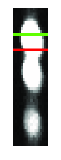
Figure 1: The left panel is a piece of arc lamp fiber spectral image of LAMOST (Cui et al. (2012)), bright spots are emission lines. The green and the red lines indicate rows where we sample the 1D profiles on the same arc emission line. The right panel illustrates normalized profiles sampled on the row with the same colors in the left. The profile difference is obvious. We can see that extraction method based on $I(x)\times I(y)$ can not work properly when the profile is position dependent.

this equation indicates that the profiles along $y$ direction at different $x$ are not correlated, so that we can use the same 1D profile to extract fluxes at different wavelengths. Considering the actual optical aberration, this requirement is too rigorous (see Fig. 1).

The fourth method is the deconvolution method, which was introduced by Bolton & Schlegel (2010). The principle of this method is that if we take a 2D spectral image as the convolution of PSFs and 1D spectra, when the PSFs at all positions are known, the 1D spectra can be obtained by deconvolution. This method can eliminate the profile difference between fibers, caused by the instrument optical aberration. However, the biggest drawback of the deconvolution method, as discussed by Bolton & Schlegel (2010), is that it needs a calibration matrix made from PSFs, which is too huge to be stored in memory of common computers, leaving alone computation. In this paper, we will give a new solution scheme to solve this problem. We also try to apply the deconvolution method to simulations with noise and find that the method is very sensitive to noise, that is, the solution is very unstable when noise is induced. In this paper, we also describe how to partly solve the noise problem by adding a Tikhonov item in our method.

This paper is organized as following: In Section 2, we introduce how to construct the PSFs from the arc lamp lines. Then in Section 3, our objective functions and algorithm are discussed. Computation tests on simulations with noise and serious cross talk as well as real telescope data will be illustrated in Section 4. The last section is our conclusion and discussion.

2 Constructing PSFs

Due to instrument aberration, PSFs at different positions on a CCD image are different. To fully sample the actual PSFs on the CCD chip, non-blended emission lines at all positions on the CCD is necessary. This condition is hard to be satisfied without an optical frequency comb. Instead, we can sample basic PSFs from the arc lamp emission lines which are sparsely distributed along the wavelength direction. Since the PSFs change smoothly with position, for positions where there is no emission line, the PSF can be linearly interpolated from those basic PSFs.

We select single lines from an arc lamp image. These arc lines should have high SNR and the distances between them should be as short as possible. Weak arc lines can be improved with another longer exposure. Then we calculate the centroid $(x,y)$ of each good arc line, where $y$ is the coordinate in the spatial direction and $x$ is in the wavelength direction. The PSF of each arc line is normalized and then fitted with a uniform B-spline surface. Then a basic PSF is gotten.

Assuming $PSF_{0}(x_{0},y_{0})$ is the PSF with center $(x_{0},y_{0})$, $PSF_{1}(x_{1},y_{1})$ and $PSF_{2}(x_{2},y_{2})$ are two closest basic PSF neighbors on different sides of $PSF_{0}$ at $(x_{1},y_{1})$ and $(x_{2},y_{2})$ respectively. To calculate $PSF_{0}$ from $PSF_{1}$ and $PSF_{2}$, we firstly move $PSF_{1}$ from $(x_{1},y_{1})$ to $(x_{1},y_{0})$, and $PSF_{2}$ from $(x_{2},y_{2})$ to $(x_{2},y_{0})$, then get 2 new PSFs: $PSF^{\prime}_{1}$ and $PSF^{\prime}_{2}$. If $PSF[i,j]$ denotes the PSF in the $i$th row and the $j$th column on the CCD image, then we can get $PSF_{0}$ by the formula:

$$PSF_{0}[i,j]=\frac{x_{2}-x_{0}}{x_{2}-x_{1}}PSF^{\prime}_{1}[i,j]+\frac{x_{0}-x_{1}}{x_{2}-x_{1}}PSF^{\prime}_{2}[i,j].$$ (1)

As for the PSFs close to the image edge, we can extrapolate or replicate the PSF of the closet arc line. For the purpose of this paper, it’s not necessary to use complicated algorithm, so the later is adopted. To save compuation memory, only the PSFs of arc lines are stored as basic PSFs during the program running, other PSFs are calculated by equation 1 whenever necessary.

In some instruments, distances of neighboring fibers may be so close that PSFs can not be measured simultaneously in a single arc exposure due to fiber-to-fiber cross talk. This could be solved by masking all the other fibers on the focal plane while taking an arc exposure of a single fiber or fibers separated by large distances on the CCD chip at the same time. Combining PSFs from different exposures will give a full sample of PSFs on the CCD chip. However, the algorithm should not be applied if masking neighboring fibers is not possible for instruments with significant fiber cross talk.

3 The Objective Function and The Deconvolution Algorithm

3.1 The Objective Function

Convolved with profiles of fiber and instrument, a monochromatic light beam entering a spectrograph will end up with a bell shape PSF rather than a $\delta$ function on the CCD. A 2D fiber spectrum can be treated as a lineup of these single PSFs at different wavelengths with different intensities:

$$S(\lambda,y)=\int^{+\infty}_{-\infty}C(x)PSF_{\lambda,y}(\lambda-x,y)dx,$$ (2)

where $S(\lambda,y)$ is the count recorded by the CCD at wavelength $\lambda$ and spatial coordinate $y$, and $C(x)$ is the 1D spectrum we want to derive.

Considering cross talk between fibers in a multi-fiber spectral image, the final count $F(\lambda,y)$ at position $(\lambda,y)$ can be written as:

$$F(\lambda,y)=\sum^{N_{f}}_{i=1}S_{i}(\lambda,y)+\epsilon_{\lambda,y},$$ (3)

where $S_{i}(\lambda,y)$ is the count of the $i$th spectrum at wavelength $\lambda$ and spatial coordination $y$, $N_{f}$ is the number of fibers, and $\epsilon_{\lambda,y}$ is noise.

If we have an image of $N$ pixels in the dispersion direction and $M$ pixels in the spatial direction, then for an actual computer calculation, equation 3 can be written in a discrete form:

$$F[k,m]=\sum^{N_{f}}_{i=1}\sum^{N}_{j=1}c_{i,j}PSF_{i,j}[k,m]+\varepsilon[k,m],$$ (4)

where $F[k,m]$ is the flux at the $k$th row and $m$th column of the CCD, $c_{i,j}$ is the flux recorded at the $i$th fiber and the $j$th row and $\varepsilon[k,m]$ is the noise at the $k$th row and $m$th column.

From equation 4, we can see that it is a least-quare problem. We rewrite equation 4 in matrix form:

$$F=AC+\varepsilon,$$ (5)

where $A$ is the calibration matrix with $PSF_{i,j}[k,m]$ as its element at the $(k*M+m)$th row and the $(i*N+j)$th column, and $C$ is a vector with $c_{i,j}$ as its $(i*N+j)$th element. For convenience of description, we always assume that noise $\varepsilon$ is independent and identically distributed in this paper, other cases can be easily changed into this case by a linear transformation.

For gaussian noise, the objective function of equation 4 is:

$$\min_{c_{i,j}}\sum^{N}_{k=1}\sum^{M}_{m=1}(F[k,m]-\sum^{N_{f}}_{i=1}\sum^{N}_{j=1}c_{i,j}PSF_{i,j}[k,m])^{2}.$$ (6)

For poisson noise, the objective function of equation 4 is:

$$\min_{c_{i,j}}\sum^{N}_{k=1}\sum^{M}_{m=1}\frac{(F[k,m]-\sum^{N_{f}}_{i=1}\sum^{N}_{j=1}c_{i,j}PSF_{i,j}[k,m])^{2}}{F[k,m]}.$$ (7)

We rewrite function 6 in matrix form:

$$\min_{C}(F-AC)^{T}(F-AC),$$ (8)

and its solution is

$$C=(A^{T}A)^{-1}A^{T}F.$$ (9)

If we denote $W$ as a diagonal matrix with $\frac{1}{F[k,m]}$ as its $(k*M+m)$th diagonal element, then we can rewrite function 7 as

$$\min_{C}(F-AC)^{T}W(F-AC),$$ (10)

and its solution is

$$C=(A^{T}WA)^{-1}A^{T}WF.$$ (11)

In the case of LAMOST (Cui et al. (2012)), i.e., 250 spectra on a 4k$\times$4k image, if we directly solve equation 9 or 11 as in the paper of Bolton & Schlegel (2010), the size of the calibration matrix $A$ will be $(4k\times 250)\times(4k\times 4k)=1.6\times 10^{13}$, so a double precision will require memory about 128TBytes. Even though matrix $A$ is a sparse matrix, it can not be easily stored or computed. Therefore, we can not solve this problem directly by the least-square method. However, from function 6 and 7 we can see, they are both optimization problems. Therefore, we try to solve it by an alternative optimization method.

3.2 Algorithm

For concision of expression, we will only discuss function 8, but the following procedure is also suitable for function 10.

As discussed above, direct computation of $C$ from equation 9 will require unacceptable hardware resources. But if we begin with an initial guess of $C_{0}$, then change $C_{0}$ in a way that could reduce the value of function 8 gradually, the final solution $C$ will be found when the function converges to its global minimum. To further reduce the computation requirement, every time we only change a small block of $C$ to minimize the value of function 8 while leaving other elements fixed. Then the next block of $C$ will be changed to get another local minimum. At last, the global solution will be approached when the value of function 8 stops to decrease or the decrease is less than a given precision.

To begin the iteration process, we first chose an initial guess, $C_{0}$, and a small piece of element block in $C_{0}$, for example, the first $k$ elements ($k$ is a small integer). All the elements in this block will be changed to minimize objective function 8. Next, the $\lceil k/2\rceil+1$th$,...,\lceil k/2\rceil+k$th element of the new $C_{0}$ will be selected as the new block, elements inside the block will be modified to minimize the objective function while keeping other elements unchanged. Each time the block is shifted forward by $\lceil k/2\rceil$. When all elements in $C_{0}$ have been updated, the new $C_{0}$ will be taken as the input in the next iteration.

Since all PSFs in calibration matrix A are known, objective function 8 has only one global minimum, which is equation 9. If we keep repeating the above process, the objective function value will keep decreasing and achieve its global minimum point at last.

We denote

$$R:=F-AC_{0}$$

and

$$res:=R^{T}R.$$

For a given $C_{0}$ and a block made up of elements from the $(s+1)$th to the $(s+k)$th, let $\delta C:=(0,...,0,x_{s+1},...,x_{s+k},0,...,0)^{T}$, $X_{s}:=(x_{s+1},...,x_{s+k})^{T}$ and define the $(s+1)$th, $...,(s+k)$ th columns in $A$ as submatrix $\bar{A}$, then $A\delta C\equiv\bar{A}X_{s}$. If we change $C_{0}$ by $\delta C$, the objective function becomes

$$\begin{split}&(F-A(C_{0}+\delta C))^{T}(F-A(C_{0}+\delta C))\\ =&(R-A\delta C)^{T}(R-A\delta C)\\ =&(R-\bar{A}X_{s})^{T}(R-\bar{A}X_{s})\\ =&res-2R^{T}\bar{A}X_{s}+X_{s}^{T}\bar{A}^{T}\bar{A}X_{s}.\end{split}$$ (12)

If we let $X_{s}=(\bar{A}^{T}\bar{A})^{-1}\bar{A}^{T}R$, where the objective function achieves its local minimum in the block $X_{s}$, then the value of the objective function becomes

$$res-(R^{T}\bar{A})(\bar{A}^{T}\bar{A})^{-1}(R^{T}\bar{A})^{T}\leq res.$$

The second term in the left side of the formula is a non-negative quadratic term, this means the objective function will decrease when we change $C$ locally by $\delta C$. If we keep iterating in deferent blocks, the objective function will finally converge to its global minimum.

The algorithm can be described as following:

Step 0: Given a value $\epsilon>0$, the size of block: $k$, and the size of variable $C$: $N$, $0<k\ll N$;

Step 1: Let $C_{0}:=0$, $s:=0$, $r_{1}:=0$. For function 8, let $R:=F$ and $res:=R^{T}R$;

Step 2: If $s+k>N$, $s:=N$, goto setp 3; else let $\bar{A}$ be the submatrix consisting of the $s+1$th $,...,s+k$th columns in $A$. We denote $X_{s}:=(\bar{A}^{T}\bar{A})^{-1}\bar{A}^{T}R$. Let $r_{1}:=r_{1}+2R^{T}\bar{A}X_{s}-X_{s}^{T}\bar{A}^{T}\bar{A}X_{s}$ ; $(c_{s+1},...,c_{s+k})^{T}:=(c_{s+1},...,c_{s+k})^{T}+X_{s}$; $R:=R-\bar{A}X_{s}$ and $s:=s+\lceil k/2\rceil+1$; goto step 2;

Step 3: If $s-k<0$, $s:=0$, then go to step 4; else let $\bar{A}$ be the submatrix consisting of the $s-k+1$th $,...,s$th columns in $A$. We denote $X_{s}:=(\bar{A}^{T}\bar{A})^{-1}\bar{A}^{T}R$. Let $r_{1}:=r_{1}+2R^{T}\bar{A}X_{s}-X_{s}^{T}\bar{A}^{T}\bar{A}X_{s}$ ; $(c_{s-k+1},...,c_{s})^{T}:=(c_{s-k+1},...,c_{s})^{T}+X_{s}$; $R:=R-\bar{A}X_{s}$ and $s:=s-\lceil k/2\rceil-1$;

Step 4: $res:=res-r_{1}$; If $r_{1}<\epsilon$, stop; else let $r_{1}=0$, goto step 2;

We call this algorithm the Direct Deconvolution Algorithm, or DDA, hereafter.

Since $k$ is small, $\bar{A}X_{s}$ in the algorithm can be sparsely stored and calculated. In principle, the algorithm can deal with an image of any size with the PSFs dependent on positions.

In addition, for a multi-processor computer, if we use one processor to calculate a single fiber at a time, this algorithm can be easily transferred into a parallel algorithm. For example, the size of our constructed LAMOST PSFs is 15 pixels $\times$ 15 pixels, if the distances between fibers are all greater than 8 pixels, then the odd fibers do not affect each other, neither do the even fibers. Then the following computation scheme could be applied: we first use processors to compute the odd fibers in parallel, after all the odd fibers have been computed, the even fibers will be computed in parallel. The above parallel computation process will be iterated until the solution is found. In general, if the minimal distance between the fibers is $D$, we can divide all the fibers into $\lceil\frac{15}{D}\rceil$ groups. We denote $\lceil\frac{15}{D}\rceil\triangleq G$, and $i=1,2,...,250$ as the sequence numbers of the 250 fibers. The $g$th group consists of fibers with $i\ mod\ G=g$, where $g=0,1,2,...,G-1$. Thus, fibers in the same group have no cross talk, our parallel algorithm can be applied in every group.

4 Computation tests

Throughout this paper, the computer to test our algorithm is a MacBook Pro with OS Windows XP, Intel (R) Core (TM) i7, 2.67GHz CPU and 2G memory. The programming language is VC++ 6.0.

4.1 Applied to a simulated 2D image based on LAMOST data

To test our algorithm, we have constructed a simulation 2D image based on LAMOST data. 33 emission lines per fiber from a LAMOST arc image are selected as basic PSFs to construct a $4K\times 4K$ CCD image with 250 fibers. 250 input 1D spectra are extracted from a LAMOST target image by AEM while the spectral traces are derived from the corresponding flat field image. The size of each PSF is 15 pixels $\times$ 15 pixels. Each input 1D spectrum (see Fig.2) is convolved with these PSFs along each spectral trace to generate a 2D spectrum for one fiber, then a 2D image with 250 fibers.

In the computation process, the memory occupied is less than 300M Bytes, most of which is used for storing the original and residual images. To avoid singular matrix during computation when the viable block is too big, we set the size of the viable block to 20.

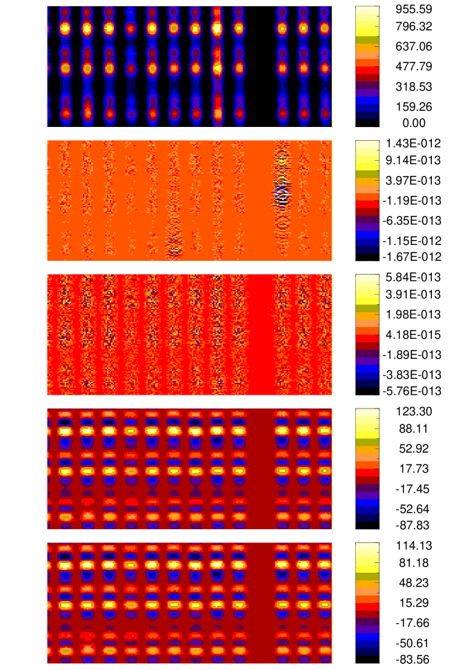
Figure 3: The top panel is a piece of simulation image, we apply different methods to this simulation image, the residuals are shown in the lower 4 panels. From the 2nd to the bottom panels are the residuals of the DDA algorithm with $\epsilon=10^{-2}$, the DDA with $\epsilon=10^{-4}$, the PFM and the AEM, respectively. Different colors represent count level on the CCD image as indicated by the color bars on the right. Compared with the PFM and the AEM, residuals of the deconvolution method are extremely small, especially around the region of emission lines.

Two tests are run following the steps described in section 3.2, the computation precision $\epsilon$s are set to $10^{-2}$ and $10^{-4}$, respectively. After running the program for 7,074 and 17,989 seconds, the results can be seen in Fig.3. The top panel of Fig.3 shows the input simulation image, the lower 2 panels show the residuals after the spectra are extracted with $\epsilon=10^{-2}$ and $10^{-4}$ respectively. For comparison, we put the 2D residual of the PFM in the fourth panel and the residual of the AEM in the bottom panel. From the corresponding color bars we can see that the residuals are extraordinarily small for our deconvolution method, and there are no obvious residuals around the emission lines in the 2nd and the 3rd panels. In contrast, the traditional PFM and AEM leave about 5$\sim$7% residuals around strong emission lines. Fig.4 shows the absolute values of the differences between the input and the extracted spectrum. The upper 2 panels show the residuals of our deconvolution method with different $\epsilon$. Only one of the 250 spectera is shown to illustrate our results. We have checked all the other spectra, they are all at the similar residual level to the spectrum shown in Fig.4. As we can see, the residual is very small with about 2 hours computation when we set $\epsilon$ to $10^{-2}$, and they are almost negligible but with a longer computation time when $\epsilon$ is set to $10^{-4}$. We also plot the residuals by the PFM and AEM in the lower two panels. Compared with the much larger residuals of the PFM and AEM, our method shows great advancement.

As can be seen from the top panel of Fig.4, the absolute values of the residuals at the beginning part of the spectrum are relatively larger than the residuals after the first 500 pixels. This is because that the calculation begins from one end of each spectrum in order of pixels. As described in 3.2, in each process of calculation, there is a block of $\lceil k/2\rceil$ pixels overlapping with the previous block. Results of these $\lceil k/2\rceil$ pixels in the previous block will be the input of the corresponding pixels in the current block. This guarantees that the solutions of conjunct blocks are related. Thus residuals in the later pixels will be smaller since their initial input had been processed closer to the final solution than the beginning part. The residual of the beginning part will be reduced if the program iterates long enough time, as shown in the second panel of Fig.4.

4.2 Applied to simulations with cross talk

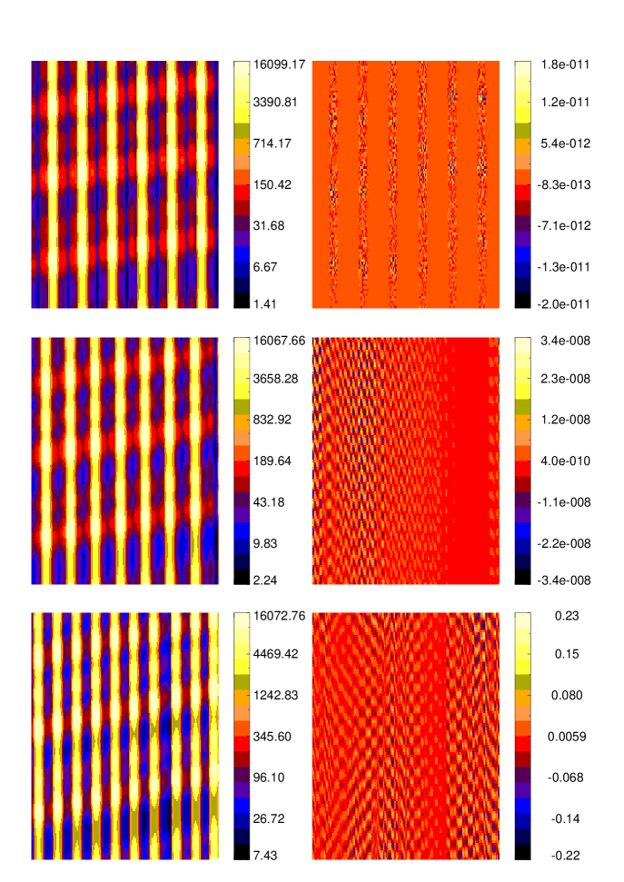
Figure 5: From top to bottom, the fiber distances in each row are set to 10, 8 and 6 pixels, respectively. Panels on the left column are pieces of simulated 2D images. Every 3 spectra, there is a spectrum 100 times stronger than its neighbors, only the bright fibers can be seen due to high contrast. Panels on the right column are the corresponding residuals after the algorithm runs for about 2 hours. Counts are represented by colors as indicated by color bars.

In the above simulations, the distances between fibers were set to the same as LAMOST, about 15-16 pixels. The size of each PSF is 15 pixels $\times$ 15 pixels and the FWHM (Full Width at Half Maximum) is about 6 pixels, so fiber-to-fiber cross talk in the above simulations is very small. To test our algorithm on images with serious cross talk, we construct 3 images using the same method discussed above but with the distances between fibers shrunk to about 10, 8 and 6 pixels, respectively (see Fig.5). We put 250 fibers in each image, the size in wavelength direction is kept as 4K pixels, so the image sizes are not the same for different fiber distances. Since the FWHM of LAMOST PSF is about 6 pixels, we do not try to simulate distances less than that. To study the influence of bright fibers on their neighbors, every 3 spectra, there is a spectrum with its flux 100 times stronger than its neighbors.

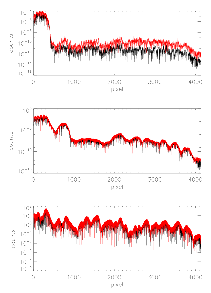
Figure 6: Absolute values of 1D residuals after the algorithm runs for about 2 hours ($\epsilon\sim 10^{-2}$). From top to bottom, panels illustrate absolute values of residuals of two 1D spectra extracted from 2D images with fiber distance about 10, 8 and 6 pixels, respectively. In each panel, the red spectrum is the residual of the bright fiber and the black spectrum is its neighbor with flux 100 times weaker.

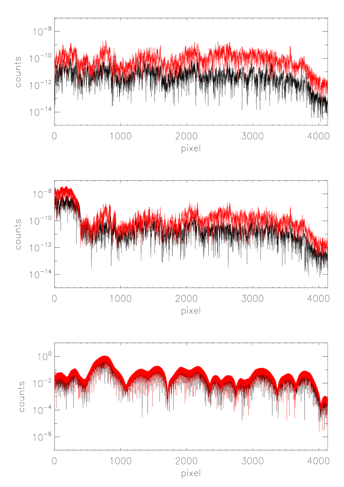
Figure 7: The same residuals as Fig.6, but for the program running for about 5 hours ($\epsilon\sim 10^{-4}$).

The program runs about 2 hours by setting $\epsilon$ to about $10^{-2}$, 2D and 1D residuals are shown in Fig.5 and Fig.6 respectively. Only two of the spectra (a bright fiber and its faint neighbor) are shown in Fig.6 to represent the common situation. From these two figures we can see: Firstly, both 1D and 2D residuals are small and acceptable. The residuals increase when fiber distance decreases, but not in a linear tendency. In fact, the residual grows much faster as the distance decreases to the extreme case, 6 pixels. Secondly, residuals of the bright fiber and its faint neighbor are on the similar level and the influence of the bright fiber on its neighbor is negligible in our method. Thirdly, as discussed in Section 4.1, residuals at the beginning parts of the 1D spectra (Fig.6) are larger than in the rest parts. They could be reduced by setting computation precision $\epsilon$ to a smaller value but with longer execution time. As shown in Fig.7, residuals at the beginning part are greatly reduced after the program runs about 5 hours when $\epsilon$ is set to about $10^{-4}$.

4.3 Comparison with Bolton & Schlegel’s method

To compare with the method of Bolton & Schlegel, a piece of 1D spectrum, with only 1,000 pixels, is convolved with LAMOST PSFs to generate a 2D image of one fiber. Then we use the DDA and the method in Bolton & Schlegel (2010) to deconvolute the 2D image respectively. Results are shown in Fig.8, we can see that our method can achieve higher accuracy than that of Bolton & Schlegel (2010). When calculating an inverse matrix, calculation error is accumulated, so a larger matrix leads to a bigger calculation error. The calibration matrix (see equation 9 and 12) in our method is much smaller than Bolton & Schlegel’s, so the calculation accuracy of its inverse can be higher than theirs. Meanwhile, calculation of large calibration matrix is very time consuming. It tooks about 123 seconds for Bolton & Schlegel’s method to run, while only 3 seconds for the DDA. Therefore, the DDA has better performance in both calculation accuracy and computation time.

4.4 Applied to simulations with poisson noise

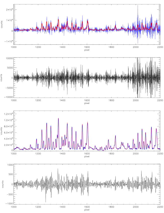
Figure 10: From top to bottom: the first panel shows the input spectrum (red curve) and the spectrum extracted by the DDA from the noise-added image shown in Fig.9 (blue curve); the second panel shows the difference between the two spectra in the first panel, from which we can see the influence of noise on the DDA is enormous; the third panel shows the spectrum extracted by the TDA (blue curve) and the same input spectrum as in the top panel (red curve); the last panel shows the difference between the two spectra in the third panel. Comparing the second panel with the fourth panel, noise introduced by the DDA is greatly suppressed by the Tikhonov regularization. To make a close view of the spectra, only a part of the full wavelength coverage is displayed here.

In the above simulations, noise is not considered, yet in actual observations, noise is inevitable. Deconvolution is an ill-posed problem, its result is very sensitive to noise. From the upper 2 panels of Fig.10 we can see that if we use the DDA to directly extract an image with noise, the spectrum will be dominated by noise. Many people (e.g. Starck et al. (2002), Puetter et al. (2005), Davies & Kasper (2012) and references therein) have discussed how to minimize the noise influence. Here we will use Tikhonov (1963) and Tikhonov & Arsenin (1977) regularization methods to control the noise. Introducing the first derivative as regularization item in the Tikhonov method, function 6 could be rewritten as:

$$\min_{c_{i,j}}\sum^{N}_{k=1}\sum^{M}_{m=1}(F[k,m]-\sum^{N_{f}}_{i=1}\sum^{N}_{j=1}c_{i,j}PSF_{i,j}[k,m])^{2}+\sum^{N_{f}}_{i=1}\sum^{N-1}_{j=1}\alpha_{i,j}(c_{i,j+1}-c_{i,j})^{2},$$ (13)

where $\alpha_{i,j}\geq 0$ is a weight to adjust the regularization item $(c_{i,j+1}-c_{i,j})^{2}$. We can rewrite equation 13 in matrix form:

$$\min_{C}(F-AC)^{T}(F-AC)+(\Gamma C)^{T}\alpha(\Gamma C),$$ (14)

where $\Gamma$ is the Tikhonov matrix consisting of 250 submatrix blocks on its diagonal. In each submatrix, the diagonal element $(k,k),(k=1,2,...,N-1)$ is -1, the element $(k,k+1),(k=1,2,...,N-1)$ is 1, and all the other elements are 0. $\alpha$ is a diagonal matrix consisting of 250 submatrix blocks, in the $i$th submatrix block, the diagonal element $(j,j),(j=1,2,...,N-1)$ is $\alpha_{i,j}$.

For an initial guess $C_{0}$, we define the same variables: $\delta C$, $X_{s}$, $\bar{A}$, $R$ and $res$ as in section 3.2, define the $s+1$ th, $...,s+k$ th columns in $\Gamma$ as submatrix $\bar{B}$, then $A\delta C\equiv\bar{A}X_{s}$, $\Gamma\delta C\equiv\bar{B}X_{s}$. Substituting the variables above into objective function 14, we could write the function in a new form:

$$\begin{split}&(F-A(C_{0}+\delta C))^{T}(F-A(C_{0}+\delta C))+(\Gamma(C_{0}+\delta C))^{T}\alpha(\Gamma(C_{0}+\delta C))\\ =&(R-\bar{A}X_{s})^{T}(R-\bar{A}X_{s})+(\Gamma C_{0}+\bar{B}X_{s})^{T}\alpha(\Gamma C_{0}+\bar{B}X_{s})\\ =&res-2R^{T}\bar{A}X_{s}+X_{s}^{T}\bar{A}^{T}\bar{A}X_{s}+(\Gamma C_{0})^{T}\alpha(\Gamma C_{0})+2C_{0}^{T}\Gamma^{T}\alpha\bar{B}X_{s}+X_{s}^{T}\bar{B}^{T}\alpha\bar{B}X_{s}\\ =&res+(\Gamma C_{0})^{T}\alpha(\Gamma C_{0})-2(R^{T}\bar{A}-C_{0}^{T}\Gamma^{T}\alpha\bar{B})X_{s}+(X_{s}^{T}\bar{A}^{T}\bar{A}X_{s}+X_{s}^{T}\bar{B}^{T}\alpha\bar{B}X_{s}).\end{split}$$ (15)

If we let $X_{s}=(\bar{A}^{T}\bar{A}+\bar{B}^{T}\alpha\bar{B})^{-1}(\bar{A}^{T}R-\bar{B}^{T}\alpha\Gamma C_{0})$, where the objective function achieves its local minimum in the block $X_{s}$, and denote $RES=res+(\Gamma C_{0})^{T}\alpha(\Gamma C_{0})$, then the value of the objective function becomes:

$$RES-(\bar{A}^{T}R-\bar{B}^{T}\alpha\Gamma C_{0})^{T}(\bar{A}^{T}\bar{A}+\bar{B}^{T}\alpha\bar{B})^{-1}(\bar{A}^{T}R-\bar{B}^{T}\alpha\Gamma C_{0})\leq RES.$$ (16)

Similar to section 3.2, the second term in the left side of the function is a non-negative quadratic term, so the objective function will keep decreasing for every small block $X_{s}$ in each iteration until the decrease is smaller than a given precision, the objective function will finally converge close to its global minimum. Because $\Gamma$ is a sparse matrix with non-zero elements all on the primary and the higher second diagonal, and $\alpha$ is also a sparse matrix with non-zero elements all on the diagonal, thus $\bar{B}^{T}\alpha\bar{B}$ and $\bar{B}^{T}\alpha\Gamma C_{0}$ can be sparsely stored and calculated.

During the computation process, $\Gamma_{d}$ denotes the decrement of the Tikhonov item in each iteration, $r_{1}$ denotes the decrement of $res$, other symbols are the same as defined above. We then change the DDA slightly, and rewrite it as following:

Step 0: Given a value $\epsilon>0$, the size of block: $k$, and the size of variable $C$: $N$, $0<k\ll N$;

Step 1: Let $C_{0}:=0$, $s:=0$. For function 14, let $R:=F$, $res:=R^{T}R$, $\Gamma_{d}:=0$, $r_{1}:=0$, $RES:=res$;

Step 2: If $s+k>N$, $s:=N$, goto setp 3; else let $\bar{A}$ be the submatrix consisting of the $(s+1)$th$,...,(s+k)$th columns in $A$, and $\bar{B}$ be a submatrix consisting of the $(s+1)$th, $...,(s+k)$th columns in $\Gamma$. We denote $X_{s}=(\bar{A}^{T}\bar{A}+\bar{B}^{T}\alpha\bar{B})^{-1}(\bar{A}^{T}R-\bar{B}^{T}\alpha\Gamma C_{0})$. Let $r_{1}:=r_{1}+2R^{T}\bar{A}X_{s}-X_{s}^{T}\bar{A}^{T}\bar{A}X_{s}$ ; $\Gamma_{d}:=\Gamma_{d}-(2C^{T}_{0}\Gamma^{T}\alpha\bar{B}X_{s}+X^{T}_{s}\bar{B}^{T}\alpha\bar{B}X_{s})$; $(c_{s+1},...,c_{s+k})^{T}:=(c_{s+1},...,c_{s+k})^{T}+X_{s}$; $R:=R-\bar{A}X_{s}$ and $s:=s+\lceil k/2\rceil+1$, goto step 2;

Step 3: If $s-k<0$, $s:=0$, then go to step 4; else let $\bar{A}$ be the submatrix consisting of the $(s-k+1)$th $,...,s$th columns in $A$, $\bar{B}$ be a submatrix consisting of the $(s-k+1)$th $,...,s$th columns in $\Gamma$. We denote $X_{s}=(\bar{A}^{T}\bar{A}+\bar{B}^{T}\alpha\bar{B})^{-1}(\bar{A}^{T}R-\bar{B}^{T}\alpha\Gamma C_{0})$. Let $r_{1}:=r_{1}+2R^{T}\bar{A}X_{s}-X_{s}^{T}\bar{A}^{T}\bar{A}X_{s}$; $\Gamma_{d}:=\Gamma_{d}-(2C^{T}_{0}\Gamma^{T}\alpha\bar{B}X_{s}+X^{T}_{s}\bar{B}^{T}\alpha\bar{B}X_{s})$; $(c_{s-k+1},...,c_{s})^{T}:=(c_{s-k+1},...,c_{s})^{T}+X_{s}$; $R:=R-\bar{A}X_{s}$ and $s:=s-\lceil k/2\rceil-1$;

Step 4: $res:=res-r_{1}$ and $RES:=RES-r_{1}-\Gamma_{d}$; If $r_{1}+\Gamma_{d}<\epsilon$, stop; else let $r_{1}=\Gamma_{d}=0$, goto step 2.

We call this algorithm the Tikhonov Deconvolution Algorithm, or TDA, here after.

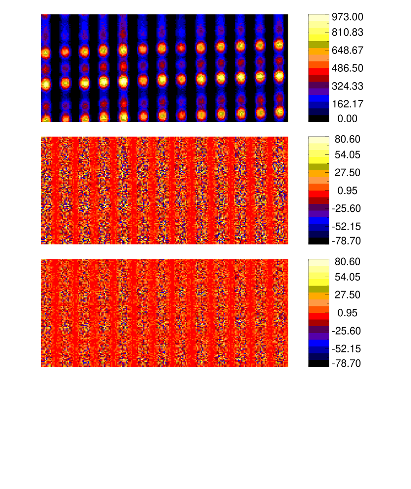
Figure 9: The top panel is the simulation 2D image with poisson noise, the middle panel is the residual of the DDA and the bottom panel is the residual of the TDA. Pixel counts are represented by different colors, as indicated by color bars on the right. The mean of the DDA and the TDA residuals are -0.0028 and 0.0026 respectively, and the standard deviations of the DDA and the TDA residuals are 12.23 and 12.75 respctively, so the 2D residuals of the two methods are almost the same.

To test the TDA, we generate a simulation image similar to that in Section 4.1, except that poisson noise is added to each pixel on the 2D image. Then the 1D spectra are extracted by the DDA and the TDA. In the TDA, all the diagonal elements of $\alpha$ are set to 0.001. Results are shown in Fig.9 and Fig.10. 2D residual images in Fig.9 show little difference between the DDA and the TDA, while compared with the DDA, the noise level in the 1D TDA result is greatly suppressed by the Tikhonov regularization, as show in Fig.10.

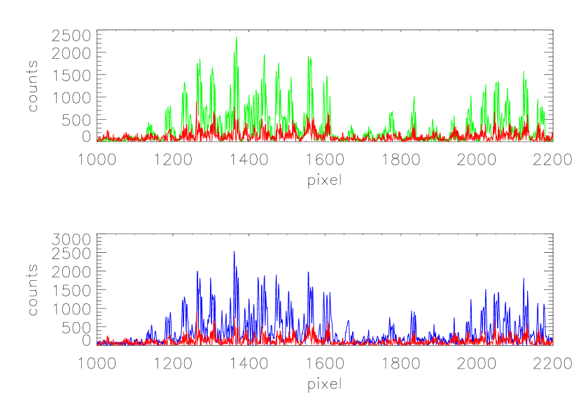
Figure 11: To compare the residual of the spectra extracted from the noise-added image by different extraction methods, we show the absolute value of the AEM residual (green curve) in the upper panel and the absolute value of the PFM residual in the lower panel (blue cure), the absolute value of the TDA residual are plotted in red in both panels. Compared with the AEM and the PFM, the residual of the TDA is the smallest.

We also extracted the noise-added 2D image by the AEM and the PFM. For comparison, absolute values of 1D residuals of different methods are shown in Fig.11. From the figure, we can see, compared with the AEM and the PFM, residual of the TDA is smaller, so 1D spectra extracted by the TDA are the most reliable.

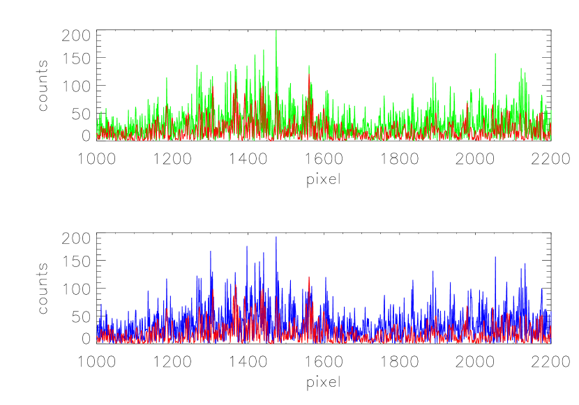
Figure 12: The same residual plots as Fig.11, but to compare the noise level of different extraction methods in the same resolution, both the input spectrum and the spectrum extracted by the TDA are degenerated to the resolution of the AEM and the PFM by convolving with a gaussian profile. Compared with the AEM and the PFM, the influenced of noise in the TDA is much less even if the resolution is the same.

In the simulation image, the distances between LAMOST fibers(15-16 pixels) are the same as the size of the input PSF (15 pixels), then uncertainty caused by the fiber cross talk is quite small, so the noise in the TDA 1D spectra should mostly come from the method in extracting the 2D image with poisson noise. But since the TDA could extract the spectrum with the similar resolution to the input spectrum, whereas the traditional methods could not, so the large residuals in the AEM and PFM are partly from the resolution difference between the input and the output spectra. To compare the noise level of different extraction methods under the same resolution, both the input spectrum and the spectrum extracted by the TDA are degenerated to the resolution of the AEM by convolving with a gaussian profile. Then the degenerated input spectra are subtracted from the 1D spectra extracted by different methods. In Fig.12, the absolute values of residuals of the AEM, the PFM and the TDA are plotted in green, blue and red, respectively. From the figure we can see, the residual of the TDA is obviously smaller than those of the AEM and the PFM. Therefore, our Tikhonov regularization item could successfully reduce the noise influence.

4.5 Applying the TDA to simulation images with poisson noise and cross talk

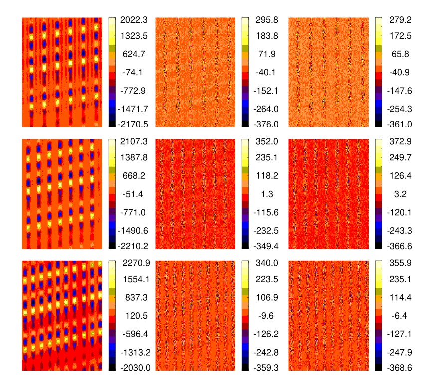
Figure 13: From left to right, columns are 2D residuals of the PFM, 2D residuals of the TDA and the input 2D poisson noise,respectively. From top to bottom, the distances between fibers in different rows are 10, 8 and 6 pixels, respectively. Comparing the medium to the right column, the 2D TDA residuals are at the similar level of the poisson noise.

To test our method under more stringent conditions, we add poisson noise to the 2D images used in subsection 4.2, on which the fibers are separated by about 6, 8 and 10 pixels, respectively. We extract the noise-added images by the TDA. The weights of the Tikhonov item, $\alpha$, are set to 0.0003 and 0.03 for the bright and the faint fibers respectively, the calculation precision $\epsilon$ is set to $10^{6}$. The 1D and the 2D residuals are shown in Fig.13 and Fig.14 respectively. For comparison, the residuals of the PFM are also plotted in these figures. We also list the corresponding SNR of each spectrum in Fig.14, here, the SNR is defined as the mean of the extracted spectrum divided by the mean square root of the difference between the extracted spectrum and the simulation input spectrum. From these figures we can see: Firstly, the 2D residuals of the TDA are comparable to poisson noise, which means that our can preserve exactly all fluxes recorded by the CCD. Secondly, both the 1D and 2D residuals of the PFM are larger than those of the TDA, the TDA spectra show much higher SNR than the PFM. Thirdly, as shown in Fig.14, the 1D spectra of faint fibers are severely polluted by their bright neighbors in all the PFM results, meanwhile, the corresponding results of the TDA show that the residuals of both faint and bright fibers are around zero. The residuals in our TDA method show no strong increase with the decreasing distance between fibers. From these simulation results we can see, the TDA is much more reliable than the traditional methods especially when there is cross talk.

4.6 Computation time

The computation times in the above simulations are 167m, 168m and 252m for fiber distances of 10, 8 and 6 pixels, respectively. As may be noticed, the calculation precision $\epsilon$ is set to $10^{6}$ in section 4.5, which is much larger than $10^{-2}$ in the noiseless simulation in section 4.2. As defined in section 3.2 and 4.4, computation precision $\epsilon$ is the threshold of the decrease of the objective function, which is summed over all pixels, that is, for our simulation with 250 fibers and 4k pixels in wavelength direction, the total number of pixels is much more than $10^{6}$ (the accurate number depends on the fiber distance, or how many pixels the 250 fibers occupy), so $\epsilon=10^{6}$ means we have an average difference much less than 1 per pixel . For the noise free simulation in section 4.2, our purpose is to test if our DDA method could work correctly with fiber-to-fiber cross talk, $\epsilon$ is set to a small value to see if the result precision could be arbitrarily high when the calculation time is long enough. For the noise added simulation in section 4.5, the calculation precision is noise dominated, so $\epsilon$ should be comparable to the noise level rather than the unnecessarily small value in section 4.2. We have made another test with $\epsilon$ set to $1.0e-20$, the results show that both the 2D and 1D residuals are at a similar level to that of $\epsilon=10^{6}$, but the computation time is 4 times longer. Beside hardware, computation time should depend on the image quality (e.g. noise, fiber number and fiber distance, etc) and input calculation parameters such as $\epsilon$, usually it is a case by case problem. It is better that we could know how to adjust the parameters to balance the computation time against the result precision. To better understand how the result precision changes with different conditions, we set $\epsilon$ to an arbitrarily low value, i.e., $1.0e-20$, then for each iteration, we output the computation time, the change of RES(see section 4.4), the SNRs of bright and faint fibers for the noise-added images of fiber distance 15, 10, 8 and 6 pixels respectively in Table 1. Only the first 9 iterations are shown in the table since the SNRs stop to increase for more iteration. From the table we can see, the computation time of each iteration are almost the same for different fiber distances, this is easy to understand since all the images we simulated contain the same number of fibers and the same size(4096 pixels) in wavelength direction, the amount of calculation is proportional to the product of the fiber number and the size in the wavelength direction, so the computation times are almost the same. For fiber distances of 15, 10 and 8 pixels, the result precision of larger fiber distance converges faster than the smaller ones, after the precision reach photon noise level ($\sim 10^{6}$), they all converge at the similar speed. But the precision decreases much slower for the extreme case, 6 pixels. If we use $\epsilon=10^{6}$ as the threshold for our computation, the 15, 10 and 8-pixels converge at a similar time, while the 6-pixels will take about 50% more time to reach the threshold, we highlight the computation times and the precisions in the table where they reach $10^{6}$ threshold. In the right part of the table, we list the SNRs of one bright fiber and its faint neighbor, the SNR is the same as defined in section 4.5. We have checked the SNRs of other fibers, the SNRs of faint fibers in the first 2 iterations change from fiber to fiber, which reflect the fact that the first result depends on the initial guess and is not stable, then the SNRs of different fiber distances increase quickly to a similar level after the first 2 iterations. The SNRs for other bright fibers are similar to those listed in the table. From the table we can see that the SNR converges to a fix value even though the calculation precision keeps decreasing after each iteration, for the fiber distances of 15, 10, 8 and 6 pixels, the SNRs converge after 3, 3, 4 and 6 iterations, respectively. The last column in Table 1 shows the SNRs of faint fibers with distance 6 pixels, we can see that the SNR increases much slowly after the 4th iteration, the corresponding precision is 6.89e8, comparing the precision and the computation time to those of 15, 10 and 8 pixels in the table, we can see that a better $\epsilon$ to balance computation time against precision may lie between $10^{7}$ and $10^{8}$. From those tests we can see that for an image with noise, we could set $\epsilon$ to a value that the average precision in each pixel does not exceed noise, usually 1 per pixel should be a lower limit. Once the precision threshold is set, except for the extreme cross talk, our method converge after 2 to 3 iterations, so the computation time does not depend so much on fiber distance for most cases.

4.7 Applying the TDA to real LAMOST data

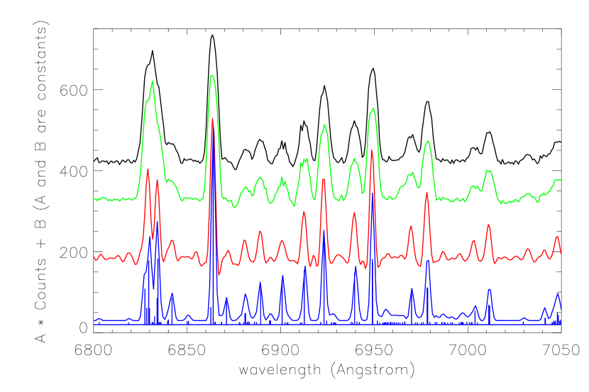
Figure 15: Results of extracting an actual LAMOST image. The spectra extracted by the AEM, the PFM and the TDA are plotted in black, green and red, respectively. The blue spectrum is a composite spectrum by convolving a gaussian profile with sky emission lines fluxes from Hanuschik (2003). We also plot the sky emission lines with relative fluxes and positions from Hanuschik (2003) in the bottom. Each spectrum is scaled and offset arbitrarily in y axis for clarity.

Now we apply our TDA to extract an actual LAMOST image. Fig.15 shows the 1D spectra extracted by the AEM(black curve), the PFM(green curve) and the TDA(red curve) from the same LAMOST 2D image, respectively. Most of the features in the spectra are sky emission lines. We also plot a composite spectrum (blue curve) by convolving a gaussian profile ($\sigma$ =1 pixel, $\sim 0.7$Å for LAMOST ) with the flux of sky emission lines from Hanuschik (2003). Relative fluxes and positions of those sky emission lines are indicated by vertical blue lines in the bottom.

From Fig.15 we can see:

Firstly, some emission lines indiscriminate in the AEM and the PFM results are clearly resolved by our method, for example, the strong emission line in the black curve around $\lambda$6830 is clearly separated into two peaks in the red curve, which are OH $\lambda$6829.5 and a blend line of OH $\lambda$6832.7 and $\lambda$6834.4. Other lines like $\lambda$6842.0, $\lambda$6871.1, $\lambda$6894, $\lambda$7041.5 and emission lines between 6975Å and 7000Å are all clearly resolved by our method, as can be seen by comparing to the blue composite spectrum. Compared to the composite spectrum, the TDA result has similar resolution(R$\sim$4200), which is 3 times higher than the AEM and the PFM results(R$\sim$1000).

Secondly, some ambiguous bifurcate peaks in the AEM and the PFM such as $\lambda$6912.6, $\lambda$6900.8, $\lambda$6969.9 and $\lambda$7003.9 are explicitly detected as single peaks by our method, which indicates that our result has higher SNR than those of the AEM and the PFM.

Thirdly, carefully comparing the red spectrum with the black, green and blue spectra, we find some weak suspicious emission lines around strong peaks, such as $\lambda$6855, $\lambda$6918 and $\lambda$6943, we think these features are most possibly caused by our Tikhonov regularization method, although the features of the underlying object can not be completely ruled out. Current Tikhonov item we adopted may produce wavy features around strong peaks, the influence of noise could not be completely eliminated. We will leave how to further constrain the noise influence in the deconvolution method for a future work.

5 Conclusion and Discussion

In this paper, we present a practical calculation scheme to extract 1D spectra from 2D images. Because of instrument optical aberration, PSFs at different positions of a CCD image are mostly different. To sample PSFs, we use emission lines on the arc image to generate discrete basic PSFs, then we use B-spline surfaces to represent the smooth basic PSF contours. By interpolating these basic PSFs, PSFs at non-emission-line region can be calculated. During the calculation process, only the smooth basic PSFs are stored in the memory, other PSFs can be calculated when necessary, so the requirement of memory is reduced.

Due to its huge requirement of computation resources, it is impossible to solve the objective function directly by the least-square method described in Bolton & Schlegel (2010). To solve this problem, we try to reduce the objective function in a small variable block in one calculation step, thus only a small amount of memory is needed. The objective function could converge to its global minimum by gradually decreasing the variable blocks to their local minimum. Thus, our calculation scheme can solve the problem with common calculation resources.

Based on our calculation scheme, we apply the Direct Deconvolution Method to extract simulation 2D images without noise. Results show that our methods could extract the 1D spectra in a precision that traditional methods could not achieve, even if fiber-to-fiber cross talk is significant.

Deconvolution methods are sensitive to noise. To suppress the noise influence, we introduce a Tikhonov item into the objective function. Then we apply the TDA to simulations with poisson noise. Results show that the TDA can extract the most reliable 1D spectra compared with the AEM and the PFM. It can correctly extract the spectrum with extreme cross talk, even for the faint fibers with fluxes 100 times lower than their neighbors.

We also apply the TDA to an actual LAMOST 2D image. Compared with the AEM and the PFM, the TDA can extract 1D spectra with both higher SNR and resolution. Theoretically, our algorithm discussed in this paper can be applied to a 2D image of any size and PSFs with any shape, even there is serious cross talk between fibers.

We further consider how to set precision parameter $\epsilon$ to balance the computation time against the result precision, and find that setting the calculation precision similar to the noise level should be a reasonable choice. Because our method converges very fast, for images with not so extreme cross talk, the computation time does not depend so much on fiber distance, usually in 2 to 3 iterations, the result will be around the peak SNR. For our simulation with 250 fibers and 4k pixels in wavelength direction, the computation times are about 2 hours for the images with fiber distance greater than 6 pixels and 3.5 hours for 6 pixels. Moreover, our algorithm could be easily transferred to a parallel algorithm, and the computation speed will be boosted.

In summary, compared with the traditional PFM and AEM, deconvolution method is the most consistent with physical process that 2D spectra are recorded by the CCD, so it can extract the most accurate fluxes from a 2D image, especially for multi-fiber spectra. Beside these, spectra extracted by our deconvolution method have higher resolution and SNR, so it is the most promising extraction method.

However, there are still some uncertainties on weak features around strong emission lines in the 1D spectra extracted by the TDA. Laborious efforts are still needed to solve the problem of noise influence. Besides the TDA, there are many other methods in the literature to attenuate the noise influence in signal processing, such as the linear regularized methods, the Bayesian methodology and the wavelet-based deconvolution methods (see Starck et al. (2002)). To study how to attenuate the noise influence on the deconvolution method will be the topic of our future work.

Table 1: Computation time and calculation precision in each iteration for images with different fiber distances

	Computation time(s)				Precision (difference of RES, see section4.4))				SNR(Brihgt Fiber)				SNR(Faint Fiber)
	15	10	8	6	15	10	8	6	15	10	8	6	15	10	8	6
1	2487	2467	2520	2472	2.35e13	2.35e13	2.35e13	2.30e13	3.58	3.55	3.57	3.62	4.57	1.38	0.17	0.04
2	5035	5015	5030	5032	2.95e9	3.50e9	3.58e10	6.28e11	15.07	14.74	15.04	14.16	4.58	4.74	4.19	0.80
3	7550	7507	7557	7535	2.12e7	2.13e7	7.89e7	2.01e10	16.34	16.18	16.70	16.06	4.58	4.71	4.71	4.16
4	10057	9997	10085	10027	2.16e5	2.62e5	3.65e5	6.89e8	16.27	16.14	16.68	16.02	4.58	4.71	4.70	3.98
5	12555	12490	12602	12575	4.27e3	4.37e3	4.50e3	2.39e7	16.25	16.13	16.67	16.00	4.58	4.71	4.70	4.27
6	15057	14977	15087	15120	84.9	84.9	87.2	9.55e5	16.25	16.13	16.67	16.00	4.58	4.71	4.70	4.30
7	17552	17470	17600	17662	1.94	1.93	1.99	4.15e4	16.25	16.13	16.67	16.00	4.58	4.71	4.70	4.31
8	20097	20017	20092	20167	4.90e-2	4.89e-2	5.05e-2	1.86e3	16.25	16.13	16.67	16.00	4.58	4.71	4.70	4.31
9	22592	22570	22590	22707	1.35e-3	1.35e-3	1.40e-3	7.75	16.25	16.13	16.67	16.00	4.58	4.71	4.70	4.31

Figure 2: One of the input 1D spectra used to generate the 2D simulation image. It is the red part of a LAMOST spectrum. As we can see, there are many strong OH sky emission lines. These lines will help us to evaluate how our deconvolution method works on reliability, SNR and resolution.

Figure 4: This figure shows the absolute values of the difference between the input spectrum and the spectrum extracted by different methods. From top to bottom, the methods are: the DDA with $\epsilon=10^{-2}$, the DDA with $\epsilon=10^{-4}$, the PFM and the AEM, respectively. Comparing with the traditional PFM and AEM methods, we can see that the residuals of deconvolution method are negligible.

Figure 8: The top panel is the input 1D spectrum used to generate 2D image; the middle panel is the difference between the input spectrum and the spectrum extracted by Bolton & Schlegel’s method; the bottom panel is the difference between the input spectrum and the spectrum extracted by the DDA. Comparing the lower two panels, the accuracy of our result is much higher than Bolton & Schlegel’s.

Figure 14: 1D residuals from images in Fig.13. The left and right columns show 1D residuals of one of the bright fibers and its faint neighbor respectively. From top to bottom, the distances between fibers are 10, 8 and 6 pixels, respectively. In each panel, the red spectrum is the residual of the TDA and the black is the residual of the PFM. We also calculate the average SNRs of the extracted spectra, which are marked with the corresponding colors in each panel.

References

- Ballester et al. (2000) Ballester, P., Modigliani, A., Boitquin, O., et al., 2000, The Messenger, 101, 31
- Bolton & Schlegel (2010) Bolton, A. S. & Schlegel, D. J., 2010, PASP, 122, 248
- Cui et al. (2012) Cui, X. Q., Zhao, Y. H., Chu, Y. Q., et al., 2012, RAA, 12, 1197
- Davies & Kasper (2012) Davies, R. & Kasper, M., 2012, ARA&A, 50, 305
- Horne (1986) Horne, K., 1986, PASP, 98, 609
- Hynes (2002) Hynes, R. I., 2002, A&A, 382, 752
- Kelz et al. (2006) Kelz, A., Verheijen, M. A. W., Roth, M. M., et al. 2006, PASP, 118, 129
- Lebouteiller et al. (2010) Lebouteiller, V., Bernard-Salas, J., Sloan, G. C., et al., 2010, PASP, 122, 231
- Marsh (1989) Marsh, T. R., 1989, PASP, 101, 1032
- Mukai (1990) Mukai, K., 1990, PASP, 102, 183
- Piskunov & Valenti (2002) Piskunov, N. E. & Valenti, J. A., 2002, A&A, 385, 1095
- Puetter et al. (2005) Puetter, R. C., Gosnell, T. R., Yahil, A., 2005, ARA&A, 43, 139
- Robertson (1986) Robertson, J. G., 1986, PASP, 98, 1220
- Sánchez (2006) Sánchez, S. F., 2006, Astronomische Nachrichten, 327, 850
- Sharp & Birchall (2010) Sharp, R. & Birchall, M. N., 2010, PASA, 27, 91
- Starck et al. (2002) Starck, J. L., Pantin, E., Murtagh, F., 2002, PASP, 114, 1051
- Tikhonov (1963) Tikhonov, A. N., 1963, Soviet Mathematics Doklady, 4, 1624
- Tikhonov & Arsenin (1977) Tikhonov, A. N. & Arsenin, V. Y., 1977, Solutions of Ill-posed Problems, New York: Wiley
- Verschueren & Hensberge (1990) Verschueren, W. & Hensberge, H., 1990, A&A, 240, 216
- Hanuschik (2003) Hanuschik, R. W., 2003, A&A, 407, 1157