Resilience for Multigrid Software at the Extreme Scale

Abstract

Fault tolerant algorithms for the numerical approximation of elliptic partial differential equations on modern supercomputers play a more and more important role in the future design of exa-scale enabled iterative solvers. Here, we combine domain partitioning with highly scalable geometric multigrid schemes to obtain fast and fault-robust solvers in three dimensions. The recovery strategy is based on a hierarchical hybrid concept where the values on lower dimensional primitives such as faces are stored redundantly and thus can be recovered easily in case of a failure. The lost volume unknowns in the faulty region are re-computed approximately with multigrid cycles by solving a local Dirichlet problem on the faulty subdomain. Different strategies are compared and evaluated with respect to performance, computational cost, and speed up. Especially effective are strategies in which the local recovery in the faulty region is executed in parallel with global solves and when the local recovery is additionally accelerated. This results in an asynchronous multigrid iteration that can fully compensate faults. Excellent parallel performance on a current peta-scale system is demonstrated.

Keywords: fault tolerant algorithms, highly scalable multigrid, massive parallel and asynchron solvers
AMS: 65N55, 65Y05, 68Q85

1 Introduction

Future high performance systems will be characterized by millions of compute nodes that are executing up to a billion of parallel threads. This compute power will be extremely expensive not only with respect to acquisition costs but also due to the operational costs, whereby the energy consumption is becoming a major concern. The increasing system size results in a higher probability of failure of the components of the HPC-system [16], and thus fail-safe performance is one of the new challenges in extreme scale computing.

Faults can be classified in fail-stop and fail-continue, also called hard and soft errors, respectively, see, e.g., [15, 17]. In the first case, the process stops, e.g., due to a permanent node crash or incorrect execution path which interrupts the program and results in a loss of the state of the process. In the case of soft errors, the process continues but the failure affects the execution through “bit-flips” (transient errors). Fault tolerance techniques can be categorized in hardware-based fault tolerance (HBFT) [39, 42], system software-based fault tolerance (SBFT) [8, 10, 12, 26, 53], and algorithm-based fault tolerance (ABFT) [15, 19, 27, 35, 38]. For a general overview and a classification, we refer to [16, 17, 18].

Achieving resilience is costly, since it always requires some form of redundancy, and thus a duplication of system resources and extra energy. In particular, traditional checkpoint strategies must collect and transfer the data regularly from all compute nodes and store the data to backup memory [24, 36, 41, 47]. In large systems, this may be too expensive and slow. Consequently, algorithmic alternatives are required. It is only natural that the most efficient resilience techniques will have to exploit specific features of the algorithms.

Under the assumption that the failure can be detected, such ABFT strategies implement the resilience in the algorithm itself and thus guarantee reliable results. Originally, ABFT was proposed by Huang and Abraham [35] for systolic arrays where checksums monitor the data and are used for a reconstruction. Later on, it was extended to applications in linear algebra such as addition, matrix operations, scalar product, LU-decomposition, transposition and in fast Fourier transformation [2, 11, 21, 37]. The work by Davies and Chen [25] deals with fault detection and correction during the calculation for dense matrix operations. For sparse matrix iterative solvers, such as SOR, GMRES, CG-iterations the previously mentioned approaches are not suitable due to a possible high overhead [48] and were extended by [1, 15, 20, 44, 50]. In [23], Cui et al. exploit the structure of a parallel subspace correction method such that the subspaces are redundant on different processors, and the workload is efficiently balanced.

At this time, the immediate detection and the replacement of the faulty components is not part of the standard message passing interface (MPI), however, fault tolerant MPI versions, such as Harness FT-MPI [28] or ULFM [8, 9] are under development. They do also not yet provide an instant reporting of the failure, but may do so in future versions when the hardware itself is extended to better support such features. For the purposes of this paper, we assume that such extensions are already available.

In this article, we thus consider fail-stop errors as they may occur in iterative schemes when solving discretized elliptic partial differential equations. We focus on the design of fault tolerant parallel geometric multigrid methods since geometric multigrid methods are well-known for their asymptotic optimal complexity and excellent parallel efficiency [13, 22, 32, 31, 33, 40, 51]. The influence of soft faults on an algebraic multigrid solver was studied in [19]. Similar to [23], we pursue fault tolerance strategies for hard faults that

• converge when a fault occurs, assuming it is detectable,

• minimize the delay in the solution process,

• minimize computational and communication overhead.

In order to compensate for a hard fault, we decouple the faulty part from the intact part and exploit the fact that only relatively little of the data must be stored redundantly so that a special recovery process can reconstruct the bulk of the missing data efficiently. Furthermore, we find that the redundant data as it is required for the reconstruction of lost data is readily available in suitably designed data structures. These data structures can be found in many distributed memory parallel multigrid solvers that use a domain partitioning and ghost nodes for communicating.

Our design goal is to minimize the time delay in an iterative solver that seems inevitable when a fault has destroyed part of its internal state. Here, however, we will show that the flexibility of modern heterogeneous architectures can be used beneficially. If the recovery is executed with powerful enough resources, the loss can in many cases be compensated completely and the time to solution experiences no delay. In other words, by using a computational superman to recover the lost state, we are able to fully compensate a fault.

The rest of our paper is organized as follows: In Sec. 2, we describe the model PDE and fault setting. The required data structure for our recovery strategies will be discussed in Sec. 3. The redundancy in the ghost layer data structures allows to combine full multigrid efficiency with tearing and interconnecting strategies. In Sec. 4, we then develop local recovery strategies and study numerically their influence on the global convergence. The main algorithmic result can be found in Sec. LABEL:sec:globalrecovery. Here Dirichlet–Neumann and Dirichlet–Dirichlet coupling strategies are combined with fast hierarchical multigrid methods. The effect of the size of the faulty domain is illustrated for large scale computations. In Sec. 5, we test both new global recovery strategies on a state-of-the-art peta-scale system. To fully compensate for the fault with respect to the time to solution, we enhance the massively parallel geometric multigrid method by asynchronous components on partitioned domains.

2 Model problem and fault setting

In this section, we introduce the model PDE scenario, the notation for the geometrical multigrid solver and the fault model for which we design our recovery techniques.

2.1 Model problem and parallel multigrid solver

For the sake of simplicity, we will illustrate the methods for the Laplace equation in 3D with inhomogeneous Dirichlet boundary conditions

$$-\Delta u=0~{}~{}\mbox{in }\Omega,\qquad u=g~{}~{}\mbox{on }\partial\Omega$$ (1)

as PDE model problem. The generalization to more general boundary conditions, right hand sides or other scalar elliptic problems is straightforward. In Sec. 4, we will also present a numerical example for the Stokes system. Here, $\Omega\subset\mathbb{R}^{3}$ is a bounded polyhedral domain which is triangulated with an unstructured base mesh $\mathcal{T}_{-2}$. In the following, we will assume for simplicity that tetrahedral elements are used, but again our techniques generalize readily to hexahedral and hybrid meshes. From this initial coarse mesh, a hierarchy of meshes $\mathcal{T}:=\{\mathcal{T}_{l},~{}l=0,\ldots,L\}$ is constructed by successive uniform refinement, see, e.g., [7]. This hierarchy is used to construct the geometric multigrid solver; the choice to start with $l=0$ guarantees that there is at least one inner degree of freedom if the mesh on level $l$ is restricted to one $T\in\mathcal{T}_{-2}$.

The discretization of (1) uses conforming linear finite elements (FE) on $\mathcal{T}_{l}$ that leads canonically to a nested sequence of finite element spaces $V_{0}\subset V_{1}\subset\ldots\subset V_{L}\subset H^{1}(\Omega)$ and a corresponding family of linear systems

$$A_{l}\underline{u}_{l}=\underline{f}_{l};~{}l=0,\ldots,L,$$ (2)

where the Dirichlet boundary conditions are included. We apply multigrid correction schemes in V-cycles with standard components to (2). In particular, we use linear interpolation and its adjoint operator for the inter-grid transfer, a hybrid variant of a Gauss-Seidel updating scheme in three pre- and post-smoothing steps and a preconditioned conjugate gradient (PCG) method as coarse grid solver. For a general overview of multigrid methods, we refer to [13, 33]. In highly parallel multigrid frameworks for distributed memory architectures [3, 5, 29, 32, 51], the work load for solving PDE problems is typically distributed to different processes based on a geometrical domain partitioning. Here, the base tetrahedral mesh $\mathcal{T}_{-2}$ defines the partitioning used for parallelization. Each tetrahedron $T\in\mathcal{T}_{-2}$ is associated with a processor, and this also induces a process assignment for all refined meshes. In general, several of the coarse mesh tetrahedra would be assigned to each processor so that a good load balancing occurs. In our simple model case, all tetrahedra are equally refined and thus induce the same load, so that for the sake of simplicity, we assume that the number of processors is equal to the number of tetrahedra in $\mathcal{T}_{-2}$, i.e., we have a one-to-one mapping of base mesh tetrahedra to processors.

2.2 Fault model and pollution effect

For our study, we concentrate on a specific fault model under assumptions similar to [23, 34]. We restrict our study, for simplicity, to the case that only one processor crashes. All strategies can be extended easily to a failure of more processors, since they only rely on the locality of the fault, see also Sec. 5, where a large scale simulation with two faults at different locations will be presented.

The faulty subdomain $\Omega_{F}\subset\Omega$ is assumed to be a single open tetrahedron in $\mathcal{T}_{-2}$, and $\Omega_{I}:=\Omega\setminus\overline{\Omega}_{F}$ is called intact or healthy subdomain. Then, the intact and faulty regions are separated by an interface $\Gamma:=\partial\Omega_{I}\cap\partial\Omega_{F}$. We denote the unknowns $u_{F},~{}u_{I}$ and $u_{\Gamma}$ with respect to the subdomains $\Omega_{F},~{}\Omega_{I}$ and the interface $\Gamma$, respectively, cf. Fig. 1.

Figure 1: Domain $\Omega$ with a faulty subdomain $\Omega_{F}$, interface $\Gamma$ and intact subdomain $\Omega_{I}$.

Moreover, we assume that a failure occurs only after a complete multigrid cycle and is reported immediately. The solution values in the faulty subdomain are set to zero as initial guess. After the local re-initialization of the problem and a possible recovery step, we continue with multigrid cycles in the solution process. We focus on three categories of computational jobs in the solution process: A job in which no fault occurs is called a fault-free job, a do-nothing job is a job in which a failure occurs but no special recovery strategy is applied (besides reinitializing the solution locally to zero), and a recovery job stands for a job where recovery strategies are applied after a fault happened. We assume a process experiences a fault after $k_{F}$ cycles and count the number of iterations necessary to reach the stopping criteria (here: $10^{-15}$) in the case of a fault-free job $k_{\mbox{\small free}}$ and a faulty job with possible recovery $k_{\mbox{\small faulty}}$. To quantify the extra iterations compared to a fault-free job, we introduce a relative Cycle Advantage (CA) parameter $\kappa$ defined by

$$\kappa:=\frac{k_{\mbox{\small faulty}}-k_{\mbox{\small free}}}{k_{F}}.$$ (3)

Intuitively, we expect that $\kappa\in[0,1]$. The situation $\kappa=0$ represents the case when the recovery algorithm reaches the stopping criteria with the same number of iterations as in a fault-free job. For increasing $\kappa$, more and more additional iterations are required to reach the stopping criteria. For $\kappa=1$, $k_{F}$ additional multigrid iterations have to be carried out, and this means that essentially all information that had been accumulated before the fault, has been lost.

The following simple test setting illustrates the need for special recovery strategies. We consider a fault scenario with 16 million unknowns and a loss of 0.3 million unknowns in case of a process crash in the unit cube $\Omega=(0,1)^{3}$. The faulty subdomain is located similar to Fig. 1. On the left of Fig. 2, we show the decay of the residual within a global parallel multigrid scheme. The fault occurs after $k_{F}=5$ multigrid iterations and in the case of a do-nothing job, the residual after the fault is highly increased resulting in four additional multigrid steps to obtain a given tolerance compared to the fault-free job. Further tests show that the number of additional steps is almost always equal to $k_{F}-1$. Thus a do-nothing run results in a $\kappa$ close to one. A favorable pre-asymptotically improved convergence rate after the fault often helps to save one cycle, but besides from this, the extra cost incurred by the fault is essentially the number of cycles that have been performed before the fault. The situation becomes even worse when multiple faults occur.

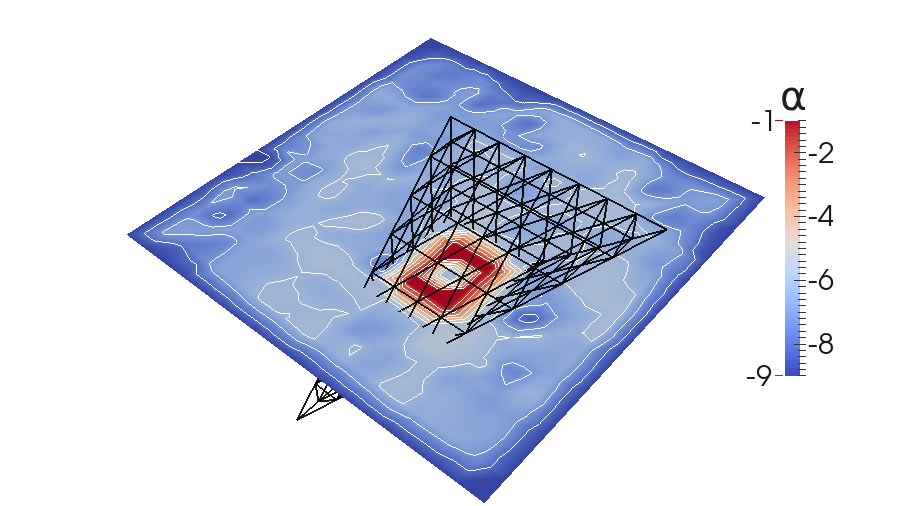
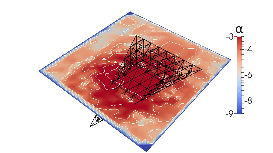
Figure 2: Residual decay (left) and residual distribution after the failure (middle) and after one additional global V-cycle (right) restricted to a cross section through the domain $\Omega$, ($\alpha:=\log_{10}(|Residual|)$).

The middle illustration in Fig. 2 visualizes the residual on a cross section through the domain directly after the failure and re-initialization. The residual distribution when one additional global multigrid cycle has been performed is given on the right. Note that large local error components within $\Omega_{F}$ are dispersed globally by the multigrid cycle. Although the smoother transports information only across a few neighboring mesh cells on each level, their combined contributions on all grid levels leads to a global pollution of the error. Though the residual decreases globally, the residual in the healthy domain $\Omega_{I}$ increases by this pollution effect. A possible remedy is based on temporarily decoupling the domains in order to avoid that the locally large residuals can pollute into the healthy domain. This is motivated by the asynchronous multilevel algorithms in [45] and leads to strategies that combine domain decomposition [43, 49, 52] and multigrid techniques. They are essentially based on hierarchical and partitioned data structures as will be discussed in the next section.

3 Software requirement for algorithmic resilience

In this section, we introduce a software architecture that is suitable to deal with faults and that supports numerical recovery procedures in the case of faults. The main ingredient for the recovery algorithms is a hybrid data structure that allows to combine multigrid mesh hierarchies with tearing and interconnecting strategies from domain partitioning. All our numerical results will be carried out within the HHG software library, [6, 30, 32], but the essential techniques can be adapted to other software concepts, since they essentially only exploit the redundancy of data in ghost layers as they are used also in other distributed memory parallel frameworks.

3.1 Hybrid hierarchical grid data structures

Often, the parallel communication of processes is organized in ghost layers (sometimes also called halos) which redundantly store copies of master data. This is a convenient technique to accommodate data dependencies across processor boundaries. Only the original master values can be written by the algorithm, and thus, once a master value has been changed, the associated ghost values must be updated to hold consistent values. We here propose a systematic construction of the ghost layer data structures that is induced by the mesh geometry.

The tetrahedra of the unstructured coarsest mesh $\mathcal{T}_{-2}$ provide natural process boundaries for all refined meshes. Note that the refined meshes will have nodes that are located on the vertices, edges, faces, and the interior of the initial elements in $\mathcal{T}_{-2}$. For two tetrahedra in 3D, this is illustrated in Fig. 4 below, but for the sake of simplicity we illustrate the concept for the 2D case in Fig. 3.

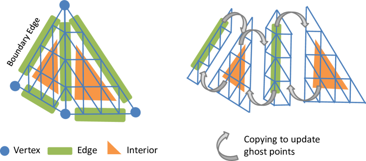
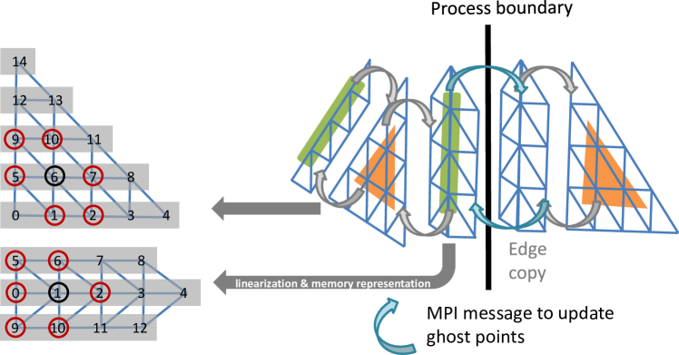
Figure 3: Top left: Two structured refined elements including grouping of the finite element nodes. Top right: Four containers for edge and interior nodes and updates of their corresponding ghost points. Bottom: Duplication of an edge container for a parallel example and synchronization via MPI. Memory representation of the data structures and one stencil for two different containers.

The upper left of Fig. 3 illustrates how first all fine mesh nodes are classified. In the upper right illustration, then the ghost layers are introduced. This is achieved by separating the two connected triangular elements, and identifying the common edge as a separate entity. For the software architecture, this classification of nodes induces a system of container data structures. In particular, there are 3D containers to hold the nodes in the interior of each $T_{i}\in\mathcal{T}_{-2}$, then 2D containers for those nodes that lie on each coarse mesh face $F_{i,j}=T_{i}\cap T_{j}$, 1D containers for the nodes that lie on the coarse mesh edges, and eventually 0D containers that hold trivially the nodes coinciding with the vertices of $\mathcal{T}_{-2}$. In a parallel setting, we will allocate all these container objects onto the different processors.

Conceptually, the next step is to introduce the ghost layers. The geometrical classification above had distributed the master copies of each node into separate containers. As indicated in Fig. 3 (top-right) (see also Fig. 4 for 3D), these containers can be enriched by ghost nodes which are copies of master nodes that are stored elsewhere. Thus all the fine grid nodes that rest on the boundary of a $T_{i}\in\mathcal{T}_{-2}$ become ghost nodes in that $T_{i}$, similarly, in the face data structure, the nodes that lie on the edges become ghost nodes, and eventually the end points of edges become ghost nodes for the edge data container. Furthermore, each of the face, edge, and node containers is enriched by one additional layer of ghost nodes that hold additional copies of master values. These extra ghost layers are essential for e.g. efficiently implementing a Gauss-Seidel iteration for the master nodes of the corresponding face container.

For the parallel implementation, we eventually introduce additional copies of the face, edge, and vertex containers so that they can be uniquely allocated on the processors of a distributed memory system. In the HHG implementation, the communication between nodes is thus split on two subtasks. One consist in updating the ghost node values in the containers that are local to a processor by simple local copy operations. The second is the actual synchronization of the interface data structures (face, edge, node) by message passing in the distributed memory system.

We remark that this construction obviously leads to a data redundancy and extra cost in data storage, but that for significantly refined meshes the additional memory cost is of lower order complexity. As we will see below, this redundancy enables efficient implementations of the parallel multilevel solver algorithms, including a systematic recovery after a fault, i.e., the numerical recovery of the data in these structures.

Note also, that these containers can be implemented using simple array data structures and can be accessed with integer indices. This can be systematically exploited to design a highly efficient implementation that avoids indirect addressing and that permits efficient vectorizable looping through the data, as indicated in Fig. 3 (lower left). Further note, that the interface data structures can also be used to implement Dirichlet or Neumann boundary conditions for those tetrahedra that lie at the domain boundary, see also Subsec. 3.2 for the resulting linear algebraic structure. We point out that in case of a fault, the master nodes of a tetrahedral container may be lost and no copies of the master values will exist anywhere. However, clearly for all of the interface structures, the above construction will provide ghost copies, from which the data can be restored.

In the following, we will design suitable recovery algorithms for this task. As a first step, we will study the resulting linear algebra structures.

3.2 Equivalent algebraic formulations

The data structure discussed in the previous subsection allows different equivalent algebraic formulations of (2) that play an important role in the following sections.

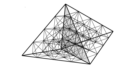
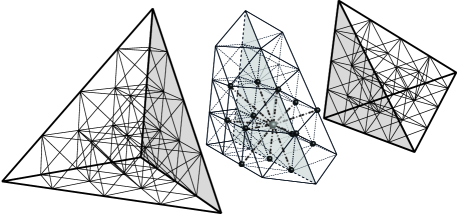
Figure 4: Two neighboring master elements (left) and ghost-layer structure of the common master face (right)

Fig. 4 illustrates the ghost-layer structure of a coarse mesh face with the master and ghost nodes of a refined mesh. For the interface container structures (faces, edges, vertices), a recovery is directly possible, since we can assume that redundant copies exist in the system. However, for the volume elements (tetrahedra), their inner nodes are not available, and thus they must be re-constructed numerically. The ghost layer structure and the associated data redundancy can be represented algebraically by rewriting (2) equivalently as

$$\begin{pmatrix}A_{II}&A_{I\Gamma_{I}}&{\bf 0}&{\bf 0}&{\bf 0}\\ {\bf 0}&\text{\bf Id}&-\text{\bf Id}&{\bf 0}&{\bf 0}\\ A_{\Gamma I}&{\bf 0}&A_{\Gamma\Gamma}&{\bf 0}&A_{\Gamma F}\\ {\bf 0}&{\bf 0}&-\text{\bf Id}&\text{\bf Id}&{\bf 0}\\ {\bf 0}&{\bf 0}&{\bf 0}&A_{F\Gamma_{F}}&A_{FF}\\ \end{pmatrix}\begin{pmatrix}\underline{u}_{I}\\ \underline{u}_{\Gamma_{I}}\\ \underline{u}_{\Gamma}\\ \underline{u}_{\Gamma_{F}}\\ \underline{u}_{F}\\ \end{pmatrix}=\begin{pmatrix}\underline{f}_{I}\\ {\bf 0}\\ {\bf 0}\\ {\bf 0}\\ \underline{f}_{F}\\ \end{pmatrix}.$$ (4)

The sub-matrices are associated with the block unknowns, in more general settings, they also depend on the basis functions and the PDE. Because of the locality of the support of the basis function, we can identify $A_{\Gamma I}$ with $A_{I\Gamma_{I}}^{\top}$ and $A_{\Gamma F}$ with $A_{F\Gamma_{F}}^{\top}$. Row 2 and row 4 in (4) guarantee the consistency of the redundant data at the interface between the master elements. Row 3 reflects, the ghost layer structures associated with the master faces. We recall that by our assumptions the data $\underline{u}_{F}$ and $\underline{u}_{\Gamma_{F}}$ are lost but $\underline{u}_{I}$ and $\underline{u}_{\Gamma_{I}}$ are still available. Although it is a priori not known what the intact domain will be, the data structure allows always such a presentation. If a processor fails which is associated with master faces, then the recovery for $\underline{u}_{\Gamma}$ can be trivially performed using the redundant information of row 2. Thus, we focus in the following only on the recovery of $\underline{u}_{F}$ and $\underline{u}_{\Gamma_{F}}$.

The ghost layer structure does not only permit access to $A_{\Gamma\Gamma}$ but also to decompose it into $A_{\Gamma_{F}\Gamma_{F}}+A_{\Gamma_{I}\Gamma_{I}}$. More precisely for each vertex on a master face, the two sub-stencils associated with $\Omega_{I}$ and $\Omega_{F}$ are available, see also Fig. 5. Having the sub-stencils at hand, we can rewrite (2) equivalently in terms of the additional flux unknown $\underline{\lambda}_{\Gamma_{I}}$ as

$$\begin{pmatrix}A_{II}&A_{I\Gamma_{I}}&{\bf 0}&{\bf 0}&{\bf 0}&{\bf 0}\\ A_{\Gamma_{I}I}&A_{\Gamma_{I}\Gamma_{I}}&{\text{\bf Id}}&{\bf 0}&{\bf 0}&{\bf 0}\\ {\bf 0}&{\text{\bf Id}}&{\bf 0}&-{\text{\bf Id}}&{\bf 0}&{\bf 0}\\ A_{\Gamma I}&{\bf 0}&{\bf 0}&A_{\Gamma\Gamma}&{\bf 0}&A_{\Gamma F}\\ {\bf 0}&{\bf 0}&{\bf 0}&-{\text{\bf Id}}&{\text{\bf Id}}&{\bf 0}\\ {\bf 0}&{\bf 0}&{\bf 0}&{\bf 0}&A_{F\Gamma_{F}}&A_{FF}\\ \end{pmatrix}\begin{pmatrix}\underline{u}_{I}\\ \underline{u}_{\Gamma_{I}}\\ \underline{\lambda}_{\Gamma_{I}}\\ \underline{u}_{\Gamma}\\ \underline{u}_{\Gamma_{F}}\\ \underline{u}_{F}\\ \end{pmatrix}=\begin{pmatrix}\underline{f}_{I}\\ {\bf 0}\\ {\bf 0}\\ {\bf 0}\\ {\bf 0}\\ \underline{f}_{F}\\ \end{pmatrix}.$$ (5)

Here $-\underline{\lambda}_{\Gamma_{I}}$ stands for the discrete flux out of $\Omega_{I}$ and into $\Omega_{F}$. It reflects a Neumann boundary condition for the intact, healthy domain. In (4) and (5), we thus find the typical algebraic structure of Dirichlet and Neumann subproblems associated with the faulty and the intact subdomain, respectively. This observation motivates the design of our parallel recovery algorithms.

                 

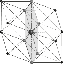
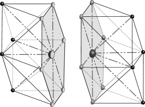
Figure 5: Stencil (left) and sub-stencil (right) structure for a vertex on a master face

4 Local recovery strategy

So far we have only considered local recovery strategies in the faulty subdomain. During the recovery, the processes in the intact subdomain are halted until the recovery in the faulty subdomain has finished. However, for the overall efficiency we cannot neglect the time spent in the recovery process. Thus, we extend our approach into two directions. Firstly, we introduce a superman strategy to speed up the local recovery process itself, and secondly we propose a global recovery such that on the faulty and intact subdomains parallel but asynchronous processes take place.

4.1 The local superman

In parallel geometric multigrid, load balancing can be often carried out with respect to the degrees of freedom. Here the situation is quite different. The multigrid iteration in the faulty subdomain must deal with a much higher residual compared to the residual on the healthy domain. To compensate for this, we use a local superman processor, i.e. we over-balance the compute power in the faulty subdomain. Technically, the additional compute resources for realizing the superman can be provided by additional parallelization. We propose here, that e.g. a full (shared memory) compute node is assigned to perform the local recovery for a domain that was previously handled by a single core. This can be accomplished by a tailored OpenMP parallelization for the recovery process. Alternatively, a further domain partitioning of $\Omega_{F}$ can be used together with an additional local distributed memory parallelization. Alternatively, one may think to exploit accelerators, such as GPUs or a Xeon Phi.

On the other hand in practice, $\Omega_{F}$ is much smaller than $\Omega_{I}$ and will typically fit in a single processor memory. Thus a suitably designed recovery process will automatically benefit from locality. In this case, the local process will be automatically faster than a global process of the same type involving full message passing communication over long distances. Moreover, in a standard multigrid implementation, the coarsest grid for $\Omega_{F}$ contains only one inner node, and thus the coarse grid problem within the local multigrid cycle is trivial to solve and does not contribute to the time per multigrid cycle. This is in contrast to large scale parallel computations, when the cost of the coarse grid solver can often not be neglected, since it may contribute $50\%$ or more of the total time to solution.

Since we here assume that local and global computation are performed simultaneously, the time for the recovery is presented as the maximum of the time spent in $\Omega_{I}$ and in $\Omega_{F}$. By introducing $\eta_{\mbox{\footnotesize super}}$ as the acceleration ratio of the cycles that can be performed simultaneously in $\Omega_{F}$, parallel to one iteration in $\Omega_{I}$, we obtain a quantitative measure for the expected speed up. This speedup can be caused by an increase of the compute power and/or an decrease of the communication overhead and a complexity decrease in the coarse grid solver. If $\eta_{\mbox{\footnotesize super}}=1$, there is no speedup, i.e., one global cycle can be performed as fast as a local one. For the ideal but practically not relevant situation $\eta_{\mbox{\footnotesize super}}=\infty$, the local recovery of Sec. 4 does not contribute to the global run time.

4.2 Dirichlet-Dirichlet recovery strategy

In the Dirichlet-Dirichlet recovery, we freeze the values $\underline{u}_{\Gamma_{I}}$ at the interface $\Gamma_{I}$. This allows to compute the two subproblems in $\Omega_{F}$ and $\Omega_{I}$ independently and consequently no communication between $\Omega_{F}$ and $\Omega_{I}$ is necessary. Thus, it is guaranteed that no defect data is polluted into the healthy subdomain during the recovery. On both subdomains, we iterate now on decoupled Dirichlet problems with boundary data on $\Gamma$ given by $\underline{u}_{\Gamma}$. Obviously, at some point we have to reconnect the two subdomains again. The algorithm for the Dirichlet-Dirichlet recovery is presented in Alg. 1

Algorithm 1 Dirichlet-Dirichlet recovery (DD) algorithm

1:Solve (2) by multigrid cycles.

2:if Fault has occurred then

3:     STOP solving (2).

4:     Recover boundary data $\underline{u}_{\Gamma_{F}}$ from line 4 in (4)

5:     Initialize $\underline{u}_{F}$ with zero

6:     In parallel do:

7:      a) Use $n_{F}$ MG cycles accelerated by $\eta_{\mbox{\footnotesize super}}$ to approximate line 5 in (4):

8:     $\qquad A_{FF}\underline{u}_{F}=\underline{f}_{F}-A_{F\Gamma_{F}}\underline{u}_{\Gamma_{F}}$

9:      b) Use $n_{I}$ MG cycles to approximate line 1 in (4)

10:     $\qquad A_{II}\underline{u}_{I}=\underline{f}_{I}-A_{I\Gamma_{I}}\underline{u}_{\Gamma_{I}}$

11:     RETURN to line 1 with new values $\underline{u}_{I}$ in $\Omega_{I}$ and $\underline{u}_{F}$ in $\Omega_{F}$.

12:end if

4.3 Dirichlet-Neumann recovery strategy

In the Dirichlet-Neumann recovery strategy, we do not freeze the interface values but treat them as Neumann boundary data in the healthy subdomain. By doing so, we use a one-directional coupling of the faulty subdomain $\Omega_{F}$ and the healthy subdomain $\Omega_{I}$. On $\Omega_{I}$ we approximate a Neumann boundary problem with static data, whereas on $\Omega_{F}$, we approximate a Dirichlet problem with dynamic boundary data. After each multigrid cycle on $\Omega_{I}$, the newly computed interface values $\underline{u}_{\Gamma_{I}}$ are asynchronously communicated via $\underline{u}_{\Gamma}$ onto $\underline{u}_{\Gamma_{F}}$. Hence, we only avoid communication from the faulty to the healthy domain but still keep communicating from the intact to the faulty subdomain. As in the case of the Dirichlet-Dirichlet recovery strategy, it is necessary to fully interconnect both subdomains after a couple of cycles. The algorithm is presented in Alg. 2.

Algorithm 2 Dirichlet-Neumann recovery (DN) algorithm

1:Solve (2) by multigrid cycles.

2:if Fault has occurred then

3:     STOP solving (2).

4:     Compute the Neumann condition from line 2 in (5):

5:     $\qquad\underline{\lambda}_{\Gamma_{I}}=-A_{\Gamma_{I}I}\underline{u}_{I}-A_{\Gamma_{I}\Gamma_{I}}\underline{u}_{\Gamma_{I}}$

6:     Initialize $\underline{u}_{F}$ with zero.

7:     In parallel do:

8:      a) Perform $n_{F}$ cycles with acceleration $\eta_{\mbox{\footnotesize super}}$:

9:            Recover/update boundary values $\underline{u}_{\Gamma_{F}}$ from line 5 in (5).

10:            Use 1 MG cycle to approximate line 6 in (5):

11:     $\qquad A_{FF}\underline{u}_{F}=\underline{f}_{F}-A_{F\Gamma_{F}}\underline{u}_{\Gamma_{F}}$

12:      b) Perform $n_{I}$ cycles:

13:            Use 1 MG cycle to approximate lines 1+2 in (5)

14:     $\qquad\begin{pmatrix}A_{II}&A_{I\Gamma_{I}}\\ A_{\Gamma_{I}I}&A_{\Gamma_{I}\Gamma_{I}}\\ \end{pmatrix}\begin{pmatrix}\underline{u}_{I}\\ \underline{u}_{\Gamma_{I}}\end{pmatrix}=\begin{pmatrix}\underline{f}_{I}\\ \underline{\lambda}_{\Gamma_{I}}\\ \end{pmatrix}$

15:            Update boundary values $\underline{u}_{\Gamma}$ from line 3 in (5).

16:     RETURN to line 1 with values $\underline{u}_{I}$ in $\Omega_{I}$, $\underline{u}_{\Gamma}$ on $\Gamma$ and $\underline{u}_{F}$ in $\Omega_{F}$.

17:end if

4.4 Comparison of the recovery strategies

In this subsection, we compare the Dirichlet-Dirichlet (DD) and Dirichlet-Neumann (DN) recovery with the local recovery strategy (LR), where calculations are only performed in the faulty subdomain while the healthy domain stays idle.

From the left to the right in Fig. 6, the three different fault geometries and macro-meshes are shown which is uniformly refined seven times for the following computations. Scenario (I) has 2 millions unknowns and the fault (red marked tetrahedron) is located with two faces at the boundary of the computational domain and affects about 16.7% of the total unknowns. Scenario (II) has 16 millions unknowns, a corruption by the fault of 2.0% (like in Subsec. LABEL:sec:AlgoPerf), and the faulty domain has one edge coinciding with the boundary. Scenario (III) has 56 millions unknowns, the faulty domain is floating in the center of the $\Omega$ and affects only 0.6% of the unknowns.

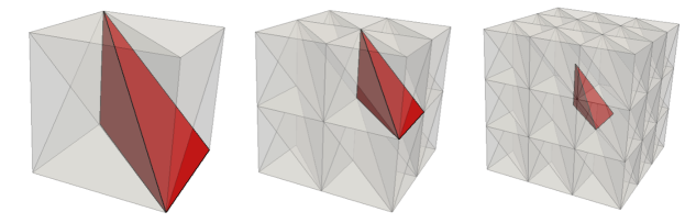
Figure 6: From left to right: Scenario (I), Scenario (II) and Scenario (III)

In Tab. 1 and Tab. 2, we present the values for the cycle advantage $\kappa$ with respect to the three different fault scenarios. We compare these strategies for two different superman speed up factors $\eta_{\mbox{\footnotesize super}}=2$ and $\eta_{\mbox{\footnotesize super}}=5$. In addition, we also illustrate the influence of $n_{I}$ in the recovery strategy before interconnecting the faulty and intact domain. Please note that the choice $n_{I}=0$ reflects a do-nothing job. We always fix $n_{F}=\lceil n_{I}*\eta_{\mbox{\footnotesize super}}\rceil$ and run the numerical tests for $n_{I}\in\{0,1,2,3,4\}$, i.e., in the case $n_{I}=3$ and $\eta_{\mbox{\footnotesize super}}=2$, we have $n_{F}=6$. To evaluate $\kappa$, we set $k_{\text{faulty}}$ to the sum of the required global multigrid cycles and $n_{I}$. We point out that in Sec. 4, we had $\eta_{\mbox{\footnotesize super}}=1$, i.e., $n_{I}=n_{F}$, and we did not add $n_{I}$ to the global multigrid cycle to get $k_{\text{faulty}}$. From the results of Sec. 4, it is now obvious that the local recovery strategy without $\eta_{\mbox{\footnotesize super}}>1$ is of no interest.

Tab. 1: Comparison of the Cycle Advantage $\kappa$ for the local, Dirichlet-Dirichlet and Dirichlet-Neumann recovery strategy for a fault after 5 iterations.

Superman speedup $\eta_{\mbox{\footnotesize super}}=2$
	Scenario (I)			Scenario (II)			Scenario (III)
$n_{I}$	LR	DD	DN	LR	DD	DN	LR	DD	DN
0	0.60	0.60	0.60	0.80	0.80	0.80	0.80	0.80	0.80
1	0.20	0.00	0.00	0.40	0.40	0.40	0.20	0.20	0.00
2	0.40	0.20	0.00	0.40	0.40	0.20	0.40	0.00	0.00
3	0.60	0.40	0.20	0.60	0.60	0.40	0.60	0.20	0.00
4	0.80	0.60	0.40	0.80	0.80	0.60	0.80	0.40	0.20

Superman speedup $\eta_{\mbox{\footnotesize super}}=5$
$n_{I}$	LR	DD	DN	LR	DD	DN	LR	DD	DN
0	0.60	0.60	0.60	0.80	0.80	0.80	0.80	0.80	0.80
1	0.20	0.00	0.00	0.20	0.20	0.20	0.20	0.00	0.00
2	0.40	0.20	0.00	0.40	0.40	0.20	0.40	0.00	0.00
3	0.60	0.40	0.20	0.60	0.60	0.40	0.60	0.20	0.00
4	0.80	0.60	0.40	0.80	0.80	0.60	0.80	0.40	0.20

In Tab. 1, the results are given for a fault after 5 global multigrid iterations. All recovery strategies can drastically reduce the delay compared to a do-nothing strategy since they can attain a considerably smaller cycle advantage $\kappa$. For Scenario (I) and Scenario (III), we can even achieve $\kappa=0$. The Scenario (III) is more relevant for applications on mid-size clusters, whereas Scenario (I) is more relevant for small desktop systems. Relevant cases for peta-scale systems will be considered in the next section. We observe a clear advantage in using a global recovery strategy instead of a local recovery strategy. In the case of the (LR) strategy, most of the machine stays idle for $n_{I}$ multigrid cycles. Only in the case of the two global recovery strategies, we fully exploit the compute power of the total system. The Dirichlet-Neumann recovery strategy is the most powerful and robust one with respect to the choice of $n_{I}$. In all cases, $n_{I}$ plays a crucial role in the overall performance. If $n_{I}$ is too large, we are over-solving the subdomain problems, if $n_{I}$ is too small, then the approximation on the faulty subdomain is too inaccurate and the global performance suffers from the pollution of the local defect into the global subdomain

Tab. 2: Comparison of the Cycle Advantage $\kappa$ for the local, Dirichlet-Dirichlet and Dirichlet-Neumann recovery strategy for a fault after 11 iterations.

Superman speedup $\eta_{\mbox{\footnotesize super}}=2$
	Scenario (I)			Scenario (II)			Scenario (III)
$n_{I}$	LR	DD	DN	LR	DD	DN	LR	DD	DN
0	0.82	0.82	0.82	0.91	0.91	0.91	0.91	0.91	0.91
1	0.64	0.64	0.63	0.82	0.82	0.82	0.64	0.64	0.64
2	0.55	0.55	0.55	0.55	0.55	0.55	0.45	0.45	0.45
3	0.36	0.36	0.36	0.45	0.45	0.45	0.36	0.36	0.36
4	0.36	0.27	0.27	0.36	0.36	0.36	0.36	0.27	0.27
5	0.45	0.36	0.27	0.45	0.45	0.36	0.45	0.27	0.27
6	0.64	0.45	0.36	0.55	0.55	0.45	0.45	0.36	0.36

Superman speedup $\eta_{\mbox{\footnotesize super}}=5$
$n_{I}$	LR	DD	DN	LR	DD	DN	LR	DD	DN
0	0.82	0.82	0.82	0.91	0.91	0.91	0.91	0.91	0.91
1	0.36	0.36	0.36	0.36	0.36	0.36	0.27	0.27	0.27
2	0.18	0.09	0.00	0.18	0.18	0.09	0.18	0.00	0.00
3	0.27	0.18	0.09	0.27	0.27	0.18	0.27	0.09	0.09
4	0.36	0.27	0.18	0.36	0.36	0.27	0.36	0.18	0.18

To obtain a better feeling for the optimal $n_{F}$ depending on $k_{F}$, we consider in Tab. 2 the situation of a fault after 11 multigrid cycles. In contrast to Tab. 1, we must select $n_{I}$ larger to get the best cycle advantage $\kappa$. This results from the fact that now the local subproblem solver on the faulty domain must counterbalance the smaller residual on the healthy domain and achieve a higher accuracy.

The best choice for all strategies seems to have a $n_{F}$ close to $k_{F}$, e.g., for a fault after $k_{F}=11$ iterations and $\eta_{\mbox{\footnotesize super}}=5$ in Tab. 1, the best choice is $n_{I}=2$ and $n_{F}=10$. The later the fault occurs, the more powerful the recovery strategy has to be. In particular without a significantly increased compute power per degree of freedom in the faulty domain compared to the healthy domain, we cannot fully compensate for the fault.

5 Parallel recovery

Now we investigate both global recovery strategies in a parallel setting on a state-of-the-art peta-scale system. Our test system is JUQUEEN, an IBM Blue Gene/Q system with a peak performance of more than $5.9$ petaflop/s. Each of the 28 672 nodes is equipped with 16 cores. Each core can execute up to four hardware threads to help hiding latencies. A five-dimensional torus network results in short communication paths within the system. The HHG software used in this article is compiled by the IBM XL C/C++ compiler V12.1 using flags -O3 -qstrict -qarch=qp -qtune=qp) and is linked to MPICH2 version 1.5. Technically, we realize the superman strategy by a logical splitting of the faulty tetrahedron and by employing additional MPI processes to perform the recovery. The software was compiled by the IBM XL C/C++ compiler V12.1 (using flags -O3 -qstrict -qarch=qp -qtune=qp) and linked to MPICH2 version 1.5.

Table 3 presents weak scaling results with $6\times(2^{l}+1)^{3}$ coarse mesh tetrahedra, $l\in\{1,2,3,4\}$. After refinement to full resolution, each coarse mesh tetrahedron contains about $2.8\cdot 10^{6}$ grid points and is assigned to one hardware thread of JUQUEEN. Hence, the ratio between faulty and healthy domain decreases from $0.6\,\%$ to $3.4\cdot 10^{-3}\,\%$ during the weak scaling sequence presented here. The first column displays the total number of unknowns in the system. In the largest computations, we solve for more than $8.2\cdot 10^{10}$ degrees of freedom on 14 743 compute cores. The numbers in the rest of the table represent the additional time-to-solution compared to a fault-free run. A negative number here means that due to the superman strategy, the computation with recovery terminates with the stopping criterion being satisfied faster than a fault-free run. As we can see from Tables 3 this surprising effect is possible due to the fact that the temporary decoupling of the subdomains reduces the communication, but clearly this kind of saving is not very significant.

Tab. 3: Additional time spans (in seconds) of different global recovery strategies during weak scaling with a fault after $k_{F}=7$ iterations.

	DD Strategy $n_{I}=1$				DN Strategy $n_{I}=1$
Size	No Rec	${\eta_{\mbox{\footnotesize super}}}=1$	$2$	$4$	$8$	${\eta_{\mbox{\footnotesize super}}}=1$	$2$	$4$	$8$
$769^{3}$	13.00	12.97	10.30	2.66	-0.02	12.98	10.30	2.66	0.02
$1\,281^{3}$	13.05	12.79	10.37	2.52	0.28	12.78	10.40	2.53	0.23
$2\,305^{3}$	13.25	10.34	7.86	2.98	0.08	10.66	7.91	2.98	0.08
$4\,353^{3}$	10.89	10.81	5.50	-0.02	0.15	10.57	5.29	-0.21	-0.83

	DD Strategy $n_{I}=2$				DN Strategy $n_{I}=2$
Size	No Rec	${\eta_{\mbox{\footnotesize super}}}=1$	$2$	$4$	$8$	${\eta_{\mbox{\footnotesize super}}}=1$	$2$	$4$	$8$
$769^{3}$	13.00	12.72	5.03	-0.10	-0.24	12.74	5.05	-0.09	-0.24
$1\,281^{3}$	13.05	12.52	5.00	-0.30	-0.03	12.53	5.01	-0.28	-0.03
$2\,305^{3}$	13.25	10.05	4.98	0.07	-0.22	10.11	5.03	0.07	-0.22
$4\,353^{3}$	10.89	7.81	2.52	2.28	2.49	7.63	2.33	-0.54	-0.35

	DD Strategy $n_{I}=3$				DN Strategy $n_{I}=3$
Size	No Rec	${\eta_{\mbox{\footnotesize super}}}=1$	$2$	$4$	$8$	${\eta_{\mbox{\footnotesize super}}}=1$	$2$	$4$	$8$
$769^{3}$	13.00	9.95	2.28	-0.36	-0.48	9.99	2.31	-0.32	-0.47
$1\,281^{3}$	13.05	9.26	2.17	-0.56	-0.31	9.70	2.15	-0.54	-0.32
$2\,305^{3}$	13.25	9.78	2.15	-0.21	-0.52	9.81	2.15	-0.21	-0.51
$4\,353^{3}$	10.89	7.53	2.21	1.99	2.16	7.27	-0.65	-0.85	-0.68

	DD Strategy $n_{I}=4$				DN Strategy $n_{I}=4$
Size	No Rec	${\eta_{\mbox{\footnotesize super}}}=1$	$2$	$4$	$8$	${\eta_{\mbox{\footnotesize super}}}=1$	$2$	$4$	$8$
$769^{3}$	13.00	9.71	2.02	1.92	1.78	9.73	2.04	1.96	1.80
$1\,281^{3}$	13.05	9.43	1.88	1.71	1.80	9.43	-0.68	-0.82	-0.59
$2\,305^{3}$	13.25	9.54	-0.75	-0.53	2.56	9.53	-0.71	-0.51	-0.79
$4\,353^{3}$	10.89	6.92	4.32	4.07	3.91	7.15	1.67	1.47	1.65

In the second column, we display the additional time for the do-nothing job. The retardation of the time-to-solution ranges from $27.5\%$ to $34.6\%$. For example, for a large problem with $4\ 353^{3}$ unknowns, the time-to-solution increases from $39.60s$ to $50.49s$. To analyze the global recovery strategies, we must realize supermen with a higher compute power than a normal processor. Here we implement supermen with $\eta_{\mbox{\footnotesize super}}\in\{1,2,4,8\}$ by replacing the single faulty processor by $\eta_{\mbox{\footnotesize super}}$ spare processors. As in the previous section, the DN strategy is more robust with respect to $n_{I}$ compared to the DD strategy. However, a superman power of $\eta_{\mbox{\footnotesize super}}=8$ does not improve the results significantly compared to $\eta_{\mbox{\footnotesize super}}=4$. Already with $\eta_{\mbox{\footnotesize super}}=4$, we can in most cases fully compensate the fault and achieve the required accuracy with no increased time-to-solution. Setting $n_{I}=1$, is not a good choice since it requires a large $\eta_{\mbox{\footnotesize super}}$ to compensate for accuracy loss in the faulty domain. The later the fault occurs the more it is important to set $n_{I}$ and thus $n_{F}$ large enough, i.e., re-couple not too early, and to have a strong enough superman. We recall that $n_{F}=\eta_{\mbox{\footnotesize super}}n_{I}$. The DN recovery strategy in combination with $\eta_{\mbox{\footnotesize super}}=4$, $n_{I}=2$ or $n_{I}=3$ yields the optimal choice with respect to time-to-solution and cost efficiency.

At this stage, we point out that the cost of the superman becomes insignificant in a large scale computation, even if 2, 4, or 8 spare processors must be kept idle until they are called for help. This is simply an effect of scale. When we use 14 743 processors, even providing 12 cores for three supermen of strength $\eta_{\mbox{\footnotesize super}}=4$ (which would be able to compensate for the unrealistic scenario of three faults in a single solve) constitutes only an extra cost of less than 0.1%.

Finally, we test in Tab. 4 a scenario where two faults at different locations occur at different times. The first processor crash happens after 5 multigrid iterations and the second one after 9. Since we select $n_{I}\leq 4$, the recovery of the first fault has finished when the second one occurs. A failure-prone cluster with many consecutive faults does not provide a suitable environment for trustable high-performance computations such that a certain interval between the crashes is reasonable. For $4\ 353^{3}$ unknowns, the time-to-solution increases form $39.60s$ to $59.34s$ and the additional consumed computation time for the scaling ranges due to the second fault now from $47.8\%$ to $55.7\%$ of the original time where no fault has occurred.

Tab. 4: Additional time spans (in seconds) of the Dirichlet-Neumann recovery strategies during weak scaling with a fault after $k_{F}=5$ and $k_{F}=9$ iterations.

		DN Strategy $\eta_{\mbox{\footnotesize super}}=4$
Size	No Rec	${n_{I}}=1$	$2$	$3$	$4$
$769^{3}$	19.21	8.01	0.05	-0.38	4.22
$1\,281^{3}$	21.27	10.58	-0.15	-0.68	3.95
$2\,305^{3}$	18.50	7.91	-0.33	-0.87	3.76
$4\,353^{3}$	19.74	5.81	2.58	4.61	9.24

We specify $\eta_{\mbox{\footnotesize super}}=4$ and study the performance with respect to $n_{I}$. For $n_{I}=1$, we obtain already a significant improvement compared to the do-nothing job. Nevertheless with $n_{I}=2$ or $n_{I}=3$, we observe much better results. As a rule of thumb we can set for moderate values of $n_{I}$, $n_{I}$ such that $n_{F}=\eta_{\mbox{\footnotesize super}}n_{I}\approx n_{I}+k_{F}-2$. This rule of thumb is based on the observation that we need roughly $k_{F}-2$ iteration to compensate for the fault in the local recovery and on the assumption that our global accuracy is still governed by the one in the faulty domain and does not suffer from the reduced communication. If this rule of thumb would require a value larger than three or four for $n_{I}$, then one should increase the superman power. If $n_{I}$ is too large then too many steps without information exchange at the interface between healthy and faulty subdomain are carried out and the multigrid acts as direct solver on the subdomains with inexact boundary data. Thus short time-to-solutions require a careful balancing of volume and surface components, and a $n_{I}$ and $n_{F}$ not too small but also not too large.

6 Conclusion and Outlook

This paper presents first insight in constructing a fault tolerant parallel multigrid solver. Hard faults result in a loss of dynamical data in a subdomain. Geometric multigrid solvers are inherently well suited to compensate such a loss of process state and to reconstruct the data based on a redundant storage scheme for numerical values only along the subdomain interfaces and using efficient recovery algorithms for the bulk of the data. To recover lost numerical values, local reconstruction subproblems with Dirichlet boundary conditions are solved approximately.

It is found that approximate solvers using a single fine grid, such as relaxation schemes or Krylov space methods, as well as conventional domain decomposition techniques with direct subdomain solvers are much too inefficient and are thus unsuitable to serve as a basis for practical fault recovery techniques. In contrast, local multigrid cycles can be used to recompute the lost data with the least numerical effort. This strategy becomes efficient in both cost and time-to-solution when the local multigrid recovery cycles are accelerated by a superman strategy, as it can be realized by an excess parallelization.

Further, we investigate methods that combine local and global processing in an asynchronous way. A Dirichlet-Dirichlet recovery or Dirichlet-Neumann recovery strategy can be used, which both iterate in the faulty subdomain and the healthy subdomain independently, until the local solution has been recovered sufficiently well. Only then the subdomains are reconnected to continue the regular multigrid solution process. Both strategies can further reduce the delay in case of a fault. For different fault scenarios, we observe that the Dirichlet-Neumann strategy should be preferred. Combined with the superman compute power on the small faulty subdomain, the global recovery techniques can result if a full numerical compensation of the fault while costing no additional compute time. The robustness and flexibility of the designed algorithms are tested on a state-of-the art peta-scale system including large scale simulation with close to $10^{11}$ unknowns. We thus believe that the superman strategy will be a viable and resource efficient approach to achieve ABFT on future exa-scale systems which may have many millions of cores.

References

- [1] E. Agullo, L. Giraud, A. Guermouche, J. Roman, and M. Zounon. Towards resilient parallel linear Krylov solvers: recover-restart strategies. Research Report RR-8324, July 2013.
- [2] J. Anfinson and F. T. Luk. A linear algebraic model of algorithm-based fault tolerance. IEEE Trans. Comput., 37(12):1599–1604, 1988.
- [3] S. Balay, S. Abhyankar, M. Adams, J. Brown, P. Brune, K. Buschelman, V. Eijkhout, W. Gropp, D. Kaushik, M. Knepley, et al. Petsc users manual revision 3.5. Technical report, Argonne National Laboratory (ANL), 2014.
- [4] R. E. Bank, B. D. Welfert, and H. Yserentant. A class of iterative methods for solving saddle point problems. Numer. Math., 56(7):645–666, 1990.
- [5] P. Bastian, M. Blatt, A. Dedner, C. Engwer, R. Klöfkorn, R. Kornhuber, M. Ohlberger, and O. Sander. A generic grid interface for parallel and adaptive scientific computing. part ii: Implementation and tests in dune. Computing, 82(2-3):121–138, 2008.
- [6] B. K. Bergen and F. Hülsemann. Hierarchical hybrid grids: Data structures and core algorithms for multigrid. Numer. Linear Algebra Appl., 11(2-3):279–291, 2004.
- [7] J. Bey. Tetrahedral grid refinement. Computing, 55(4):355–378, 1995.
- [8] W. Bland, A. Bouteiller, T. Herault, G. Bosilca, and J. J. Dongarra. Post-failure recovery of mpi communication capability: Design and rationale. Int. J. High Perform. Comput. Appl., page 1094342013488238, 2013.
- [9] W. Bland, A. Bouteiller, T. Herault, J. Hursey, G. Bosilca, and J. J. Dongarra. An evaluation of user-level failure mitigation support in MPI. Springer, 2012.
- [10] W. Bland, P. Du, A. Bouteiller, T. Herault, G. Bosilca, and J. J. Dongarra. Extending the scope of the checkpoint-on-failure protocol for forward recovery in standard MPI. Concurrency Computat.: Pract. Exper., 25(17):2381–2393, 2013.
- [11] D. L. Boley, R. P. Brent, G. H. Golub, and F. T. Luk. Algorithmic fault tolerance using the Lanczos method. SIAM J. Matrix Anal. Appl., 13(1):312–332, 1992.
- [12] G. Bosilca, A. Bouteiller, E. Brunet, F. Cappello, J. Dongarra, A. Guermouche, T. Herault, Y. Robert, F. Vivien, and D. Zaidouni. Unified model for assessing checkpointing protocols at extreme-scale. Concurrency Computat.: Pract. Exper., 26(17):2772–2791, 2014.
- [13] A. Brandt and O. E. Livne. Multigrid Techniques: 1984 Guide with Applications to Fluid Dynamics, Revised Edition. Classics in Applied Mathematics. Society for Industrial and Applied Mathematics, 2011.
- [14] F. Brezzi and J. Douglas, Jr. Stabilized mixed methods for the Stokes problem. Numer. Math., 53(1-2):225–235, 1988.
- [15] P. G. Bridges, K. B. Ferreira, M. A. Heroux, and M. Hoemmen. Fault-tolerant linear solvers via selective reliability. ArXiv e-prints, June 2012.
- [16] F. Cappello. Fault tolerance in petascale/exascale systems: Current knowledge, challenges and research opportunities. Int. J. High Perform. Comput. Appl., 23(3):212–226, 2009.
- [17] F. Cappello, A. Geist, B. Gropp, L. Kale, B. Kramer, and M. Snir. Toward exascale resilience. Int. J. High Perform. Comput. Appl., 23(4):374–388, Nov. 2009.
- [18] F. Cappello, A. Geist, S. Kale, B. Kramer, and M. Snir. Toward exascale resilience: 2014 update. Supercomput. Front. Innov., 1:1–28, 2014.
- [19] M. Casas, B. R. de Supinski, G. Bronevetsky, and M. Schulz. Fault resilience of the algebraic multi-grid solver. In Proceedings of the 26th ACM International Conference on Supercomputing, ICS ’12, pages 91–100, New York, NY, USA, 2012. ACM.
- [20] Z. Chen. Online-ABFT: An online algorithm based fault tolerance scheme for soft error detection in iterative methods. In Proceedings of the 18th ACM SIGPLAN Symposium on Principles and Practice of Parallel Programming, PPoPP ’13, pages 167–176, New York, NY, USA, 2013. ACM.
- [21] Z. Chen and J. Dongarra. Algorithm-based fault tolerance for fail-stop failures. IEEE Trans. Parallel Distrib. Syst., 19(12):1628–1641, 2008.
- [22] E. Chow, R. D. Falgout, J. J. Hu, R. S. Tuminaro, and U. Meier-Yang. A survey of parallelization techniques for multigrid solvers. In M. A. Heroux, P. Raghavan, and H. D. Simon, editors, Parallel processing for scientific computing, number 20 in Software, Environments, and Tools, pages 179–201. Society for Industrial and Applied Mathematics, 2006.
- [23] T. Cui, J. Xu, and C.-S. Zhang. An Error-Resilient Redundant Subspace Correction Method. ArXiv e-prints, Sept. 2013.
- [24] J. Daly. A model for predicting the optimum checkpoint interval for restart dumps. In Computational Science-ICCS 2003, pages 3–12. Springer, 2003.
- [25] T. Davies and Z. Chen. Correcting soft errors online in LU factorization. In Proceedings of the 22Nd International Symposium on High-performance Parallel and Distributed Computing, HPDC ’13, pages 167–178, New York, NY, USA, 2013. ACM.
- [26] S. Di, M. S. Bouguerra, L. Bautista-Gomez, and F. Cappello. Optimization of multi-level checkpoint model for large scale HPC applications. In Proceedings of the 2014 IEEE 28th International Parallel and Distributed Processing Symposium, IPDPS ’14, pages 1181–1190, Washington, DC, USA, 2014. IEEE Computer Society.
- [27] P. D. Düben, J. Joven, A. Lingamneni, H. McNamara, G. De Micheli, K. V. Palem, and T. N. Palmer. On the use of inexact, pruned hardware in atmospheric modelling. Philos. Trans. R. Soc. Lond. Ser. A Math. Phys. Eng. Sci., 372(2018), 2014.
- [28] G. E. Fagg and J. J. Dongarra. Ft-mpi: Fault tolerant mpi, supporting dynamic applications in a dynamic world. In Recent advances in parallel virtual machine and message passing interface, pages 346–353. Springer, 2000.
- [29] R. Falgout and U. Meier-Yang. hypre: A library of high performance preconditioners. Computational Science-ICCS 2002, pages 632–641, 2002.
- [30] B. Gmeiner, H. Köstler, M. Stürmer, and U. Rüde. Parallel multigrid on hierarchical hybrid grids: a performance study on current high performance computing clusters. Concurrency Computat.: Pract. Exper., 26(1):217–240, 2014.
- [31] B. Gmeiner, U. Rüde, H. Stengel, C. Waluga, and B. Wohlmuth. Towards textbook efficiency for parallel multigrid. Numer. Math. Theory Methods Appl., 8(01):22–46, 2015.
- [32] B. Gmeiner, U. Ruüde, H. Stengel, C. Waluga, and B. Wohlmuth. Performance and scalability of hierarchical hybrid multigrid solvers for Stokes systems. SIAM J. Sci. Comput., 37(2):C143–C168, 2015.
- [33] W. Hackbusch. Multi-grid methods and applications, volume 4. Springer-Verlag Berlin, 1985.
- [34] B. Harding, M. Hegland, J. Larson, and J. Southern. Scalable and fault tolerant computation with the sparse grid combination technique. ArXiv e-prints, Apr. 2014.
- [35] K.-H. Huang and J. A. Abraham. Algorithm-based fault tolerance for matrix operations. IEEE Trans. Comput., 33(6):518–528, June 1984.
- [36] J. Hursey. Coordinated checkpoint/restart process fault tolerance for mpi applications on hpc systems. PhD thesis, Indiana University, 2010.
- [37] F. T. Luk and H. Park. An analysis of algorithm-based fault tolerance techniques. J. Parallel. Distr. Com., 5(2):172–184, Apr. 1988.
- [38] K. Malkowski, P. Raghavan, and M. Kandemir. Analyzing the soft error resilience of linear solvers on multicore multiprocessors. In Parallel Distributed Processing (IPDPS), 2010 IEEE International Symposium on, pages 1–12, April 2010.
- [39] M. Maniatakos, P. Kudva, B. Fleischer, and Y. Makris. Low-cost concurrent error detection for floating-point unit (FPU) controllers. IEEE Trans. Comput., 62(7):1376–1388, July 2013.
- [40] O. A. McBryan, P. O. Frederickson, J. Lindenand, A. Schüller, K. Solchenbach, K. Stüben, C.-A. Thole, and U. Trottenberg. Multigrid methods on parallel computers - a survey of recent developments. Impact Comput. Sci. Engrg., 3(1):1–75, 1991.
- [41] A. Moody, G. Bronevetsky, K. Mohror, and B. R. De Supinski. Design, modeling, and evaluation of a scalable multi-level checkpointing system. In High Performance Computing, Networking, Storage and Analysis (SC), 2010 International Conference for, pages 1–11. IEEE, 2010.
- [42] S. S. Mukherjee, J. Emer, and S. K. Reinhardt. The soft error problem: An architectural perspective. In High-Performance Computer Architecture, 2005. HPCA-11. 11th International Symposium on, pages 243–247. IEEE, 2005.
- [43] A. Quarteroni and A. Valli. Domain Decomposition Methods for Partial Differential Equations. University Press, Oxford, 1990.
- [44] A. Roy-Chowdhury and P. Banerjee. A fault-tolerant parallel algorithm for iterative solution of the laplace equation. In Parallel Processing, 1993. ICPP 1993. International Conference on, volume 3, pages 133–140, Aug 1993.
- [45] U. Rüde. Fully adaptive multigrid methods. SIAM J. Numer. Anal., 30(1):230–248, 1993.
- [46] J. Schöberl and W. Zulehner. On Schwarz-type smoothers for saddle point problems. Numer. Math., 95(2):377–399, 2003.
- [47] F. Shahzad, M. Wittmann, T. Zeiser, G. Hager, and G. Wellein. An evaluation of different i/o techniques for checkpoint/restart. In Parallel and Distributed Processing Symposium Workshops & PhD Forum (IPDPSW), 2013 IEEE 27th International, pages 1708–1716. IEEE, 2013.
- [48] J. Sloan, R. Kumar, and G. Bronevetsky. Algorithmic approaches to low overhead fault detection for sparse linear algebra. In Proceedings of the 2012 42Nd Annual IEEE/IFIP International Conference on Dependable Systems and Networks (DSN), DSN ’12, pages 1–12, Washington, DC, USA, 2012. IEEE Computer Society.
- [49] B. F. Smith, P. E. Bjørstadt, and W. Gropp. Domain Decomposition: Parallel Multilevel Methods for Elliptic Partial Differential Equations. Universtiy Press, Cambridge, 1996.
- [50] M. K. Stoyanov and C. G. Webster. Numerical analysis of fixed point algorithms in the presence of hardware faults. Technical report, Oak Ridge National Laboratory (ORNL), Aug 2013.
- [51] H. Sundar, G. Biros, C. Burstedde, J. Rudi, O. Ghattas, and G. Stadler. Parallel geometric-algebraic multigrid on unstructured forests of octrees. In High Performance Computing, Networking, Storage and Analysis (SC), 2012 International Conference for, pages 1–11, Nov 2012.
- [52] A. Widlund and O. B. Tosseli. Domain Decomposition Methods - Algorithms and Theory, volume 34 of Series in Computational Mathematics. Springer, Berlin, 2005.
- [53] G. Zheng, C. Huang, and L. V. Kalé. Performance evaluation of automatic checkpoint-based fault tolerance for AMPI and Charm++. ACM SIGOPS Operating Systems Review, 40(2):90–99, 2006.
- [54] W. Zulehner. Analysis of iterative methods for saddle point problems: a unified approach. Math. Comp., 71(238):479–505, 2002.