Transverse Momentum Resummation for Dijet Correlation in Hadronic Collisions

Abstract

We study the transverse momentum resummation for dijet correlation in hadron collisions based on the Collins-Soper-Sterman formalism. The complete one-loop calculations are carried out in the collinear factorization framework for the differential cross sections at low imbalance transverse momentum between the two jets. Important cross checks are performed to demonstrate that the soft divergences cancelled out between different diagrams, and in particular, those associated with final state jets. The leading and sub-leading logarithms are identified. All order resummation is derived following the transverse momentum dependent factorization at this order. Its phenomenological applications are also presented.

I Introduction

Dijet production in hadronic collisions is one of the golden channels to study perturbative QCD and hadron physics in high energy experiments. In dijet events, the two jets are produced mainly in the back-to-back configuration in the transverse plane,

$$A+B\to Jet_{1}+Jet_{2}+X\ ,$$ (1)

where $A$ and $B$ represent the two incoming hadrons with momenta $P$ and $\overline{P}$, respectively, the azimuthal angle between the two jets is defined as $\phi=\phi_{1}-\phi_{2}$ with $\phi_{1,2}$ being the azimuthal angles of the two jets. There have been comprehensive analyses of the azimuthal angular correlation (or decorrelation) in dijet events produced at hadron colliders Abazov:2004hm ; Khachatryan:2011zj ; daCosta:2011ni . In the leading order naive parton picture, the Born diagram contributes to a Delta function at $\phi=\pi$. One gluon radiation will lead to a singular distribution around $\phi=\pi$, which will persist at even higher orders Nagy:2001fj . This divergence arises when the total transverse momentum of dijet (imbalance) is much smaller than the individual jet momentum, $q_{\perp}=|\vec{P}_{1\perp}+\vec{P}_{2\perp}|\ll|P_{1\perp}|\sim|P_{2\perp}|\sim P_{T}$, where large logarithms appear in every order of perturbative calculations. These large logs are normally referred as the Sudakov logarithms, $\alpha_{s}^{i}\ln^{2i-1}(P_{T}^{2}/q_{\perp}^{2})$. Therefore, a QCD resummation has to be included in order to have a reliable theoretical prediction. The goal of this paper is to derive the resummation formulas for dijet production in the kinematics of these large logarithms. A brief summary of our results has been published in Ref. Sun:2014gfa .

In the kinematics region $q_{\perp}\ll P_{T}$, the appropriate resummation method to apply is the so-called transverse momentum dependent (TMD) resummation or the Collins-Soper-Sterman (CSS) resummation Collins:1984kg . The CSS resummation was derived for the massive neutral particle production in hadronic collisions, such as the electroweak boson (or Higgs boson) production. However, due to the presence of the colored final state, the resummation of dijet production will be much more complicated. There have been theoretical progressed in the leading double logarithmic approximation (LLA), where it was found that each incoming parton contributes half of its color charge to Sudakov resummation factor Banfi:2003jj ; Banfi:2008qs ; Hautmann:2008vd ; Mueller:2013wwa . In this paper, we will go beyond the LLA to perform the resummation calculation at the next-to-leading logarithm (NLL) level. The threshold resummation for dijet production in hadronic collisions has been investigated in a series of publications by Sterman and his collaborators Kidonakis:1997gm ; Botts:1989kf . The methodology of our calculations for the TMD resummation is very similar to those studies.

We will start our derivation by evaluating the differential cross sections as a function of the imbalance transverse momentum $q_{\perp}$ at the complete one-loop order. The leading order contribution is a Delta function $\delta^{(2)}(q_{\perp})$. One-loop corrections come from four contributions: (a) virtual contributions; (b) soft gluon radiation (real); (c) jet contributions; (d) collinear gluon radiation associated with the incoming parton distributions. The virtual graphs have been studied in the literature Ellis:1985er . The jet contributions are easy to derive following the examples of inclusive jet production. In order to calculate the analytical results, we will adopt the narrow jet approximation (NJA) Mukherjee:2012uz ; Jager:2004jh , where explicit dependence on jet sizes $R_{1}$ and $R_{2}$ can be evaluated. The soft gluon (real) contribution is most difficult to calculate. This is because, not all soft gluon radiation contributes to the finite $q_{\perp}$. The radiation inside the jet will be part of the jet contribution at one-loop order and has to be excluded from soft gluon radiation contribution. In our calculations, we will apply a small offshellness for the jets in the final state to calculate the soft gluon radiation. We find that this method yield the exact same results as that using kinematic cut-off to regulate soft gluon radiation in the NJA. Collinear gluon radiation associated with incoming parton distributions also contribute to the finite imbalance transverse momentum. This part can be formulated according to the well-known DGLAP splitting. In the end, for finite and soft imbalance transverse momentum $q_{\perp}$, we add the soft gluon (real) and collinear gluon (real) contributions together, which leads to the so-called asymptotic behavior for the differential cross sections at low imbalance transverse momentum $q_{\perp}$. An important cross check of our derivation is to compare its numerical results with the dijet production codes available in public. We will carry out these comparisons in this paper. Another cross check is to demonstrate the soft divergences cancellation between real and virtual graphs. We will show these cancellations in details for the hard partonic channels in our calculations. After the cancellation, we are left with only collinear divergences associated incoming parton distributions. This indicates that we do have a consistent results for dijet production at one-loop calculations.

The large logarithms mentioned above will be evident from the complete one-loop results. Resummation of these large logarithms is the main goal of current paper. To perform the resummation, we first show that the differential cross sections at one-loop order can be factorized into the transverse momentum distributions, soft factor, and hard factors, respectively. The transverse momentum distributions follow the definitions for Drell-Yan or Higgs boson production at low transverse momentum. The soft factor will have to take into account the additional effect of gluon radiation associated with the two final state jets. The idea to construct the soft factor follows the examples of threshold resummation studied by Sterman et al. Kidonakis:1997gm .

Our resummation formula can be summarized as

$$\frac{d^{4}\sigma}{dy_{1}dy_{2}dP_{T}^{2}d^{2}q_{\perp}}=\sum_{ab}\sigma_{0}\left[\int\frac{d^{2}\vec{b}_{\perp}}{(2\pi)^{2}}e^{-i\vec{q}_{\perp}\cdot\vec{b}_{\perp}}W_{ab\to cd}(x_{1},x_{2},b_{\perp})+Y_{ab\to cd}\right]\ ,$$ (2)

where the first term $W$ contains all order resummation and the second term $Y$ comes from the fixed order corrections. $\sigma_{0}$ represents the overall normalization of the differential cross section, $y_{1}$ and $y_{2}$ are rapidities of the two jets, $P_{T}$ the leading jet transverse momentum, and $q_{\perp}$ the imbalance transverse momentum between the two jets as defined above. All order resummation for $W$ from each partonic channel $ab\to cd$ can be written as

$$W_{ab\to cd}\left(x_{1},x_{2},b\right) = x_{1}\,f_{a}(x_{1},\mu=b_{0}/b_{\perp})x_{2}\,f_{b}(x_{2},\mu=b_{0}/b_{\perp})e^{-S_{\rm Sud}(Q^{2},b_{\perp})}$$ (3)

$$\times \textmd{Tr}\left[\mathbf{H}_{ab\to cd}\mathrm{exp}\left[-\int_{b_{0}/b_{\perp}}^{Q}\frac{d\mu}{\mu}\mathbf{\gamma}^{s{\dagger}}\right]\mathbf{S}_{ab\to cd}\mathrm{exp}\left[-\int_{b_{0}/b_{\perp}}^{Q}\frac{d\mu}{\mu}\mathbf{\gamma}^{s}\right]\right]\ ,$$

where $Q^{2}=\hat{s}=x_{1}x_{2}S$, representing the hard momentum scale. $b_{0}=2e^{-\gamma_{E}}$, with $\gamma_{E}$ being the Euler constant. $f_{a,b}(x,\mu)$ are parton distributions for the incoming partons $a$ and $b$, and $x_{1,2}=P_{T}\left(e^{\pm y_{1}}+e^{\pm y_{2}}\right)/\sqrt{S}$ are momentum fractions of the incoming hadrons carried by the partons. In the above equation, the hard and soft factors $\mathbf{H}$ and $\mathbf{S}$ are expressed as matrices in the color space of partonic channel $ab\to cd$, and $\gamma^{s}$ are the associated anomalous dimensions for the soft factor (defined below). The Sudakov form factor ${\cal S}_{Sud}$ resums the leading double logarithms and the universal sub-leading logarithms,

$$S_{\rm Sud}(Q^{2},b_{\perp})=\int^{Q^{2}}_{b_{0}^{2}/b_{\perp}^{2}}\frac{d\mu^{2}}{\mu^{2}}\left[\ln\left(\frac{Q^{2}}{\mu^{2}}\right)A+B+D_{1}\ln\frac{Q^{2}}{P_{T}^{2}R_{1}^{2}}+D_{2}\ln\frac{Q^{2}}{P_{T}^{2}R_{2}^{2}}\right]\ ,$$ (4)

where $R_{1,2}$ represent the cone sizes for the two jets, respectively. Here the parameters $A$, $B$, $D_{1}$, $D_{2}$ can be expanded perturbatively in $\alpha_{s}$. At one-loop order, $A=C_{A}\frac{\alpha_{s}}{\pi}$, $B=-2C_{A}\beta_{0}\frac{\alpha_{s}}{\pi}$ for gluon-gluon initial state, $A=C_{F}\frac{\alpha_{s}}{\pi}$, $B=\frac{-3C_{F}}{2}\frac{\alpha_{s}}{\pi}$ for quark-quark initial state, and $A=\frac{(C_{F}+C_{A})}{2}\frac{\alpha_{s}}{\pi}$, $B=(\frac{-3C_{F}}{4}-C_{A}\beta_{0})\frac{\alpha_{s}}{\pi}$ for gluon-quark initial state. Here, $\beta_{0}=(11-2N_{f}/3)/12$, with $N_{f}$ being the number of effective light quarks. At the next-to-leading logarithmic level, the jet cone size enters as well Banfi:2003jj . That is the reason we have two additional factors in Eq. (4): $D_{1,2}=C_{A}\frac{\alpha_{s}}{2\pi}$ for gluon jet and $D_{1,2}=C_{F}\frac{\alpha_{s}}{2\pi}$ for quark jet. The cone size $R$ is introduced to regulate the collinear gluon radiation associated with the final state jets. Only the soft gluon radiation outside the jet cone will contribute to the imbalance $q_{\perp}$ between the two jets.

There are two important issues we will not addressed in much details. First, our resummation formalism is based on a TMD factorization argument Qiu:2007ey . However, there is a potential contribution at order of $\alpha_{s}^{3}$ which violates the general TMD factorization Collins:2007nk ; Vogelsang:2007jk ; Mulders:2011zt ; Catani:2011st ; Mitov:2012gt . It was found, in particular, certain diagrams in dijet production in hadronic collisions can not be factorized into the simple universal TMDs. In terms of resummation coefficients, this will affect the coefficient $A^{(3)}$ in Eq. (4). In our numeric calculations, we will include both $A^{(1)}$ and $A^{(2)}$ coefficients in the resummation formula (see detailed discussions in Sec. IIC). Though we do not expect that the factorization violating effect will affect much the results to be presented below, it will be useful to estimate the size of factorization breaking effect in some future work.

Second, we derive our results, in both collinear and TMD approaches, by adopting the narrow jet approximation. With that, we are able to demonstrate the explicit cancellation of soft divergences from various parts of analytical calculation, and to express the resummation Sudakov form factor in an analytic form in terms of the jet sizes. Although the derivation itself is not limited to NJA, we find that the differential cross section expressions are much simplified under the NJA. How to extend our results to the case without NJA is very interesting subject. It is worthwhile to come back to this question in the future. However, in current paper, we will carry out our calculations with the NJA.

The rest of this paper is organized as follows. We will dedicate Secs. II-V to the calculations of the differential cross sections at low $q_{\perp}$ in the collinear factorization approach. In Sec. II, we start with a brief introduction of the leading order results in which the overall normalization factor for each production channel is presented. In Sec. III, we discuss the generic features to evaluate the one-loop corrections to $W(b_{\perp})$. This includes virtual graph contributions, jet contributions in the real gluon radiation, collinear gluon radiation associated with the incoming partons, and the soft gluon radiation which contributes to finite $q_{\perp}$. Since the soft gluon radiation is the most important contributions for dijet production, we dedicate Sec. IV to show the details of our calculations. In Sec. V, we compare the asymptotic results for dijet production to the fixed order calculation published in the literature. The asymptotic behavior for dijet production is calculated by summing the soft gluon radiation and collinear gluon radiation derived in Secs. III and IV. In Sec. VI, we derive the TMD factorization and resummation. In particular, we will show that the collinear calculations from Secs. III-IV at the one-loop order can be factorized into the TMDs, hard and soft factors. The latter factors are expressed in a matrix form, where they are written in terms of the color space for every partonic channel. The resummation is achieved by solving the relevant renormalization equations. In Sec. VII, we perform the phenomenological studies based on our resummation formalism. We conclude our paper in Sec. VIII.

II Dijet Production at the Leading Order

Dijet production at the leading order can be calculated from partonic $2\to 2$ processes,

$$a(p_{1})+b(p_{2})\to c(k_{1})+d(k_{2})\ ,$$ (5)

where $p_{1,2}$ and $k_{1,2}$ are momenta for incoming and outgoing two partons. Schematically, we draw the diagrams in Fig. 1.

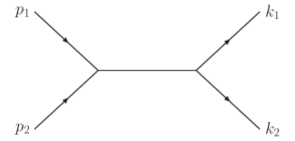
Figure 1: Schematic diagram for dijet production at the leading order, with incoming parton momenta: $p_{1}$ and $p_{2}$, and outgoing momenta: $k_{1}$ and $k_{2}$, respectively.

The partonic channels include the following subprocesses:

$$q_{i}q_{j}\to q_{i}q_{j}\ ,$$ (6)

$$q_{i}\bar{q}_{i}\to q_{j}\bar{q}_{j}\ ,$$ (7)

$$q_{i}q_{i}\to q_{i}q_{i}\ ,$$ (8)

$$qg\to qg\ ,$$ (9)

$$gg\to q\bar{q}\ ,$$ (10)

$$q\bar{q}\to gg\ ,$$ (11)

$$gg\to gg\ .$$ (12)

Their contributions can be summarized as

$$\frac{d^{4}\sigma}{dy_{1}dy_{2}dP_{T}^{2}d^{2}q_{\perp}}=\sum_{ab}\sigma_{0}x_{1}\,f_{a}(x_{1},\mu)x_{2}\,f_{b}(x_{2},\mu){h}_{ab\to cd}^{(0)}\delta^{(2)}(q_{\perp})\ ,$$ (13)

where the overall normalization of the differential cross section is $\sigma_{0}=\frac{\alpha_{s}^{2}\pi}{s^{2}}$. The partonic cross sections $h^{(0)}$ for all the production channels are listed below.

$$h_{q_{i}q_{j}\to q_{i}q_{j}}^{(0)} = \frac{4}{9}\frac{s^{2}+u^{2}}{t^{2}}\ ,$$ (14)

$$h_{q_{i}\bar{q}_{i}\to q_{j}\bar{q}_{j}}^{(0)} = \frac{4}{9}\frac{t^{2}+u^{2}}{s^{2}}\ ,$$ (15)

$$h_{q_{i}q_{i}\to q_{i}q_{i}}^{(0)} = \frac{4}{9}\left(\frac{s^{2}+u^{2}}{t^{2}}+\frac{s^{2}+t^{2}}{u^{2}}\right)-\frac{8}{27}\frac{s^{2}}{tu}\ ,$$ (16)

$$h_{gg\to q\bar{q}}^{(0)} = \frac{1}{6}\frac{u^{2}+t^{2}}{tu}-\frac{3}{8}\frac{u^{2}+t^{2}}{s^{2}}\ ,$$ (17)

$$h_{qg\to qg}^{(0)} = \frac{4}{9}\frac{u^{2}+s^{2}}{-us}+\frac{u^{2}+s^{2}}{t^{2}}\ ,$$ (18)

$$h_{gg\to gg}^{(0)} = \frac{9}{2}\left(3-\frac{ut}{s^{2}}-\frac{us}{t^{2}}-\frac{st}{u^{2}}\right)\ ,$$ (19)

where the kinematic variables $s=(p_{1}+p_{2})^{2}$, $t=(p_{1}-k_{1})^{2}$ and $u=(p_{1}-k_{2})^{2}$. As mentioned above, at the leading order, they contribute to a Delta function of $q_{\perp}$, which corresponds to the back-to-back configuration of the two jets in the transverse plane. If we translate this into the $b_{\perp}$-space, we will obtain $W(b_{\perp})$ at the leading order take the following form,

$$W_{ab\to cd}^{(0)}(b_{\perp})=x_{1}f_{a}(x_{1},\mu)x_{2}f_{b}(x_{2},\mu)h_{ab\to cd}^{(0)}\ .$$ (21)

The goal of the following three sections is to derive the one-loop corrections to $W_{ab\to cd}^{(1)}(b_{\perp})$.

III Generic Discussions on One-loop Calculations

The leading order contributions lead to a Delta function of the imbalance transverse momentum $q_{\perp}$. In the following, we will first carry out one-loop calculations of the differential cross sections at low transverse momentum. The computation is performed in the $b_{\perp}$-space, the Fourier transformed conjugate parameter to the transverse momentum $q_{\perp}$. That is to say, we will calculate $W(b_{\perp})$ at the one-loop order.

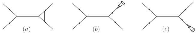
Figure 2: Schematic diagrams for virtual graph contribution (a) and final state jet contributions (b) and (c) at one-loop order. Both of them are proportional to a Delta function of the imbalance transverse momentum: $\delta^{(2)}(q_{\perp})$.

There are four types of radiative contributions at the one-loop order:

1. Virtual contributions, as shown in Fig. 2(a). These contributions have been calculated in the literature, and they are proportional to the leading order contributions, leading to a Delta function of $q_{\perp}$.

2. Real gluon radiation: Jet contributions. In the real gluon radiation, one particular contribution is also proportional to the leading order contribution, that is the jet contribution. In this case, the gluon radiation is within the jet, where its momentum is collinear to the final state parton. For example, as shown Fig. 2(b), the radiated gluon is collinear to one of the final state parton, and they form a new jet at one-loop order. Because of momentum conservation, this again leads to a Delta function of $q_{\perp}$.

3. Real gluon radiation: collinear gluon associated with incoming partons. These collinear gluons contribute to a finite $q_{\perp}$, and is proportional to $1/q_{\perp}^{2}$ multiplied by the splitting kernel of parton distribution functions. Since they originate from the incident partons, the collinear gluon contributions follow the generic structure and are easy to calculate.

4. Real gluon radiation: soft gluon contribution. Soft gluon contributions are more difficult to evaluate. They also contribute to a finite $q_{\perp}$. To evaluate this part of contribution, we apply the leading power expansion in the limit of $q_{\perp}\ll Q$. However, because the final state jets also carry color, the soft gluon radiation has to take into account the interactions among initial and final state partons. In addition, we have to exclude the soft gluon radiation within the final state (cone) jets whose contributions have already been included in the final state jet contributions. Detailed calculations will be presented in the following section.

In the rest of this section, we will go through the first three kinds of contributions, whereas the soft gluon radiation contribution will be calculated in Sec. IV.

We will carry out our calculations in the collinear factorization formalism, and apply the dimensional regulation for IR and UV divergences with dimension $D=4-2\epsilon$. Various divergences appear in individual contributions: $1/\epsilon^{2}$ represents the soft divergence, whereas $1/\epsilon$ for either soft or collinear divergence. Since we are dealing with jet production in the final states, we will also encounter the divergences associated with the jet size $R$. The explicit calculations of gluon radiation will depend on how we define the jet, i.e., the jet algorithm will play a role in formulating the one-loop corrections.

Two important cross checks will be performed in the derivations. First, the soft divergences of $1/\epsilon^{2}$ will be cancelled out completely among different terms. We notice that (1,2,4) terms listed above will have $1/\epsilon^{2}$ contributions. A crucial test of our calculations is that these $1/\epsilon^{2}$ cancel out each other. This cancellation is not trivial, since they come from different diagrams, and some with different color factors. However, we will show that the total contribution is free of soft divergence of $1/\epsilon^{2}$. Second, the divergences associated with the final state jets are also cancelled out among various terms. The collinear divergences associated with the jets are regulated by the jet sizes, and the individual contributions contain terms of $1/\epsilon\ln(1/R)$ are cancelled out in the final results. We will show that the cancellation indeed happens at this order.

Figure 3: Schematic diagrams for real gluon radiation contribution to finite imbalance transverse momentum: (a) collinear gluon radiation associated with the incoming partons; (b) soft gluon radiation outside the jet cone of final state jets.

III.1 Virtual Graphs

Virtual diagrams for dijet production in hadronic collisions have been calculated in the classic paper of Ref. Ellis:1985er . In our calculations, we will take their results.

III.2 Jet Contributions

Jet contributions contain the collinear gluon radiation and gluon to quark-antiquark splitting in the final state. The schematic diagrams have been shown in Figs. 2(b) and (c). Because we have two jets in the final state, one-loop jet corrections can come from either of the jets, as shown in Fig. 2(b) and (c), respectively. The jet contribution needs to be included to capture the collinear gluon radiation (or gluon splitting to quark-antiquark pair) within the jet cone. These gluon radiations will not change the kinematics of the parenting parton, and therefore contribute to a Delta function of $q_{\perp}$, which is similar to the virtual graph contributions. The requirement is that the two partons in the splitting process form a jet according to the jet algorithm adopted in experimental measurements. In order to derive an analytic expression with the jet cone size dependence to demonstrate the cancellations in the final results and to derive the resummation formula, we apply the narrow jet approximation (NJA) in our calculations. In particular, we follow the technique and scheme of the subtraction developed in Refs. Mukherjee:2012uz ; Jager:2004jh . The basic idea is to note that in the collinear gluon radiation limit for each final state jet,

$$|{\cal M}(2\to 3)|^{2}\approx|{\cal M}_{0}(2\to 2)|^{2}\times{\cal P}_{1\to 2}\ ,$$ (22)

where ${\cal M}(2\to 3)$ represents the scattering amplitude of $2\to 3$ subprocess, ${\cal M}_{0}(2\to 2)$ for the leading order $2\to 2$ subprocess with one of the final state parton branching into two parton final state represented by the splitting of ${\cal P}_{1\to 2}$.

Therefore, the jet contributions can be summarized as,

$$\int\frac{d^{3}k_{3}}{2E_{3}(2\pi)^{3}}\frac{E_{J}}{E_{2}}{\cal P}_{1\to 2}\ ,$$ (23)

where the factor $E_{J}/E_{2}$ accounts for the phase space difference from 3 parton final state to 2 parton final state. The phase space integral of the above equation is limited that the two partons are within the jet cone. Here the difference from jet algorithms plays a role. Using the NJA, the calculations follow what have been done in Refs. Mukherjee:2012uz ; Jager:2004jh , and in particular, we find that the gluon jet in the final state contributes

$${\cal J}^{g} = \frac{\alpha_{s}}{2\pi}\frac{1}{\Gamma(1-\epsilon)}\frac{1}{-2\epsilon}\left(\frac{P_{T}^{2}R^{2}}{4\pi}\right)^{-\epsilon}\int_{0}^{1}d\xi\left(\xi(1-\xi)\right)^{-2\epsilon}\left[f_{gg}(\xi)+f_{qg}(\xi)\right]\ ,$$ (24)

for $k_{t}$-type jet algorithm, where $R$ defines the jet cone size: $R=\sqrt{(\Delta y)^{2}+(\Delta\phi)^{2}}$. Here, $\Delta y$ and $\Delta\phi$ are the rapidity difference and azimuthal angle difference between the two partons which define the jet. In the above equation, $f_{gg}(\xi)$ and $f_{qg}(\xi)$ are splitting kernels for gluon to gluon and gluon to quark-antiquark pair Mukherjee:2012uz ; Jager:2004jh , respectively. By applying the $\overline{\rm MS}$ subtraction, we obtain,

$${\cal J}^{g}=\frac{\alpha_{s}C_{A}}{2\pi}\left[\frac{1}{\epsilon^{2}}+\frac{1}{\epsilon}\left(2\beta_{0}-\ln\frac{P_{T}^{2}R^{2}}{\mu^{2}}\right)+I^{g}\right]\ ,$$ (25)

where we have taken into account the contributions from both $g\to gg$ and $g\to q\bar{q}$ splittings. We would like to emphasize that the singular terms (double and single poles) are independent of jet algorithm. The jet algorithm dependent contributions arise from the finite term $I^{g}$. The above jet function is universal, and can be used in many other cases as well. Similarly, we find that the quark jet can be written as

$${\cal J}^{q}=\frac{\alpha_{s}C_{F}}{2\pi}\left[\frac{1}{\epsilon^{2}}+\frac{1}{\epsilon}\left(\frac{3}{2}-\ln\frac{P_{T}^{2}R^{2}}{\mu^{2}}\right)+I^{q}\right]\ .$$ (26)

In the $k_{t}$-type jet algorithms, the above mentioned $I^{q}$ and $I^{g}$ terms are already available:

$$I^{g} = \frac{1}{2}\left(\ln\frac{P_{T}^{2}R^{2}}{\mu^{2}}\right)^{2}-2\beta_{0}\ln\frac{P_{T}^{2}R^{2}}{\mu^{2}}+\frac{67}{9}-\frac{3}{4}\pi^{2}-\frac{23}{54}N_{f}\ ,$$ (27)

$$I^{q} = \frac{1}{2}\left(\ln\frac{P_{T}^{2}R^{2}}{\mu^{2}}\right)^{2}-\frac{3}{2}\ln\frac{P_{T}^{2}R^{2}}{\mu^{2}}+\frac{13}{2}-\frac{3}{4}\pi^{2}\ .$$ (28)

We note that the double logarithmic terms are independent of jet algorithm, and it is important for them to cancel in the final results, as shown in Sec. IV.

III.3 Collinear Gluon Radiation

The contributions from the collinear gluon associated with the incoming partons can be easily evaluated, and they are found to be proportional to the splitting kernel at the one-loop order:

$$\frac{\alpha_{s}}{2\pi^{2}}\frac{1}{q_{\perp}^{2}}\int\frac{dx_{1}^{\prime}}{x_{1}^{\prime}}\frac{dx_{2}^{\prime}}{x_{2}^{\prime}}f_{a^{\prime}}(x_{1}^{\prime})f_{b^{\prime}}(x_{2}^{\prime})\left[\delta(\xi_{2}-1)\xi_{1}{\cal P}_{a/a^{\prime}}^{(<)}(\xi_{1})+(\xi_{1}\leftrightarrow\xi_{2})\right]\ ,$$ (29)

where $\xi_{i}=x_{i}/x_{i}^{\prime}$ and ${\cal P}^{(<)}_{a/a^{\prime}}$ represents the splitting kernel part without the Delta function term whose effect is included in the above mentioned virtual contributions.

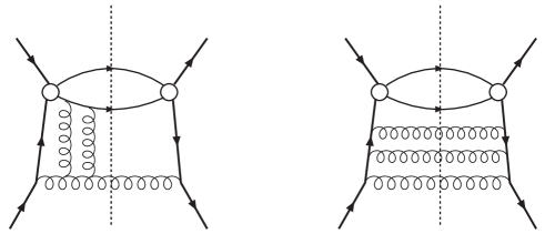
Figure 4: Example of Feynman diagrams that contribute to the TMD factorization breaking effects in two particle production via hadronic processes at ${\cal O}(\alpha_{s}^{3})$ order Collins:2007nk (left), where two gluon exchanges between the incoming/outgoing particles induce non-universality of the TMDs in this process as compared to other processes such as DIS and Drell-Yan processes. These diagrams would contribute to $A^{(3)}$ in the resummation formula. The dominant contribution at this order is illustrated in the right panel, which are factorizable and come from $A^{(1)}$ in the resummation formula.

To evaluate the contribution from soft gluon radiation requires more care. This is because we have to exclude the collinear contributions associated with the final state jet which will be factorized into a jet function and will not contribute to finite $q_{\perp}$. Before we discuss its details in the following section, we note that the TMD factorization breaking effects can appear at higher orders in two particle production at hadron colliders Collins:2007nk ; Vogelsang:2007jk ; Mulders:2011zt ; Catani:2011st ; Mitov:2012gt . These effects come from the diagrams illustrated in Fig. 4 Collins:2007nk , which belong to a nontrivial contribution at order $\alpha_{s}^{3}$ to the parton distributions. They cannot be factorized into the conventional transverse momentum dependent parton distributions, though they could contribute to the $A^{(3)}$ coefficient in the resummation formula. Since it is beyond the perturbative order (up to $\alpha_{s}^{2}$) discussed in this paper, we shall not discuss it further in this work.

IV Soft Gluon Radiation at One-loop Order

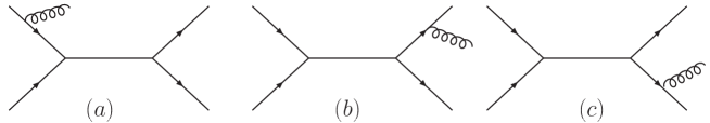
Figure 5: Soft gluon radiation contribution to finite imbalance transverse momentum $q_{\perp}$: (a) initial state radiation, and (b) and (c) final state radiations. Because we have chosen the gluon polarization vector along $p_{2}$, there is no contribution connecting to $p_{2}$ line.

For soft gluon radiations, we can apply the leading power expansion and derive the dominant contribution by the Eikonal approximation. This analysis has been applied in Ref. Mueller:2013wwa to obtain the leading double logarithmic contributions to dijet production. In the current paper, we will extend that analysis to include the subleading logarithmic contributions as well. In particular, we will derive the contributions which depend on the jet cone sizes. The relevant Feynman rules have been listed in Ref. Mueller:2013wwa . For completeness, we copy these results here. For outgoing quark, antiquark and gluon lines, we have

$$\frac{2k_{i}^{\mu}}{2k_{i}\cdot k_{g}+i\epsilon}g\ ,~{}~{}-\frac{2k_{i}^{\mu}}{2k_{i}\cdot k_{g}+i\epsilon}g\ ,~{}~{}\frac{2k_{i}^{\mu}}{2k_{i}\cdot k_{g}+i\epsilon}g\ ,$$ (30)

respectively, where $k_{i}$ represents the momentum of the outgoing particles. For incoming quark, antiquark and gluon lines, we have,

$$-\frac{2p_{1}^{\mu}}{2p_{1}\cdot k_{g}-i\epsilon}g\ ,~{}~{}\frac{2p_{1}^{\mu}}{2p_{1}\cdot k_{g}-i\epsilon}g\ ,~{}~{}\frac{2p_{1}^{\mu}}{2p_{1}\cdot k_{g}-i\epsilon}g\ ,$$ (31)

respectively, where $p_{1}$ represents the momentum for the incoming particle.

Following Ref. Mueller:2013wwa , we choose the physical polarization for the soft gluon along the incoming particle $p_{2}$. Therefore, the soft gluon radiation from the incoming particle $p_{2}$ vanishes with this polarization choice. From that, we can derive the soft gluon radiation contribution easily, with the polarization tensor for the radiated gluon,

$$\Gamma^{\mu\nu}(k_{g})=\left(-g^{\mu\nu}+\frac{k_{g}^{\mu}p_{2}^{\nu}+k_{g}^{\nu}p_{2}^{\mu}}{k_{g}\cdot p_{2}}\right)\ .$$ (32)

For example, from the amplitude squared of the soft gluon radiation terms in the above, we have

$$\frac{2p_{1}^{\mu}}{2p_{1}\cdot k_{g}}\frac{2p_{1}^{\nu}}{2p_{1}\cdot k_{g}}\Gamma_{\mu\nu} = S_{g}(p_{1},p_{2})\ ,$$ (33)

$$\frac{2k_{1}^{\mu}}{2k_{1}\cdot k_{g}}\frac{2k_{1}^{\nu}}{2k_{1}\cdot k_{g}}\Gamma_{\mu\nu} = S_{g}(k_{1},p_{2})\ ,$$ (34)

$$\frac{2k_{2}^{\mu}}{2k_{2}\cdot k_{g}}\frac{2k_{2}^{\nu}}{2k_{2}\cdot k_{g}}\Gamma_{\mu\nu} = S_{g}(k_{2},p_{2})\ ,$$ (35)

where $S_{g}(p,q)$ is a short-handed notation for

$$S_{g}(p,q)=\frac{2p\cdot q}{p\cdot k_{g}q\cdot k_{g}}\ .$$ (36)

Similarly, we derive the interferences between them,

$$2\frac{2k_{1}^{\mu}}{2k_{1}\cdot k_{g}}\frac{2p_{1}^{\nu}}{2p_{1}\cdot k_{g}}\Gamma_{\mu\nu} = S_{g}(k_{1},p_{2})+S_{g}(p_{1},p_{2})-S_{g}(k_{1},p_{1})\ ,$$ (37)

$$2\frac{2k_{2}^{\mu}}{2k_{2}\cdot k_{g}}\frac{2p_{1}^{\nu}}{2p_{1}\cdot k_{g}}\Gamma_{\mu\nu} = S_{g}(k_{2},p_{2})+S_{g}(p_{1},p_{2})-S_{g}(k_{2},p_{1})\ ,$$ (38)

$$2\frac{2k_{1}^{\mu}}{2k_{1}\cdot k_{g}}\frac{2k_{2}^{\nu}}{2k_{2}\cdot k_{g}}\Gamma_{\mu\nu} = S_{g}(k_{1},p_{2})+S_{g}(k_{2},p_{2})-S_{g}(k_{1},k_{2})\ .$$ (39)

In order to evaluate the contributions from soft gluon radiation, we integrate out the phase space of the gluon whose transverse momentum leads to the imbalance between the two jets, e.g.,

$$g^{2}\int\frac{d^{D-1}k_{g}}{(2\pi)^{D-1}2E_{k_{g}}}\delta^{(2)}(q_{\perp}-k_{g\perp})S_{g}(p_{1},p_{2})\ ,$$ (40)

where we have chosen dimensional regulation for the phase space integral. The derivation of the above term is straightforward, by noticing that the lower limit in the longitudinal momentum fraction integral,

$$\int_{x_{min}}^{1}\frac{dx}{x}\frac{1}{k_{g\perp}^{2}}\ ,$$ (41)

where we have defined $x$ as momentum fraction of $p_{1}$ carried by the soft gluon. Because of momentum conservation, we have lower limit for the $x$-integral: $x_{min}=\frac{k_{g\perp}^{2}}{Q^{2}}$. Therefore, the above integral leads to the following leading contribution,

$$\frac{1}{q_{\perp}^{2}}\ln\frac{Q^{2}}{q_{\perp}^{2}}\ .$$ (42)

Substituting the above equation into Eq. (40), we have

$$g^{2}\int\frac{d^{D-1}k_{g}}{(2\pi)^{D-1}2E_{k_{g}}}\delta^{(2)}(q_{\perp}-k_{g\perp})S_{g}(p_{1},p_{2})=\frac{\alpha_{s}}{2\pi^{2}}\frac{1}{q_{\perp}^{2}}\left(2\ln\frac{Q^{2}}{q_{\perp}^{2}}\right)\ .$$ (43)

Because there is no $\epsilon=(4-D)/2$ term in the $dx$ integral, we have taken $D=4$ in the above equation. The other terms are more difficult to calculate, because the above phase space integral will contain jet contributions which have already been taken into account by the above mentioned jet functions. To avoid double-counting, we have to subtract this part of contribution. That means the phase space integral has to exclude the jet (cone) region. It is interesting to note that the amount of this exclusion does not depend on jet algorithm. This is because, here we are considering the soft gluon radiation, whereas the jet algorithm mainly focuses on the collinear gluons associated with the jet.

IV.1 Out of the Jet-cone Radiation

As a general discussion, let us take the example of one term,

$$\int\frac{d^{D-1}k_{g}}{2E_{k_{g}}}\delta^{(2)}(q_{\perp}-k_{g\perp})S_{g}(k_{1},p_{1})=\int d^{D-2}k_{g\perp}\delta^{(2)}(q_{\perp}-k_{g\perp})\int\frac{d\xi_{1}}{\xi_{1}}\frac{2}{(k_{g\perp}-\xi_{1}k_{1\perp})^{2}}\ ,$$ (44)

where $k_{1\perp}$ represents the transverse momentum for the final state jet, and $\xi_{1}=k_{g}\cdot p_{1}/k_{1}\cdot p_{1}$. Clearly, there is collinear divergence associated with the jet. That means, if the gluon radiation is within the jet cone, it will generate a collinear divergence. In order to regulate this collinear jet divergence, we can limit the phase space integral to require that the gluon radiation being outside of the jet cone. With this restriction, there will be no divergence associated with the jet. Instead, the jet (cone) size $R$ will be introduced to regulate the collinear divergence from the jet.

There are different ways to regulate the above integral. The main task is to identify the need of introducing jet (cone) size. In the above example, the integral diverges when $k_{g}$ is parallel to $k_{1}$, where the invariant mass of $k_{1}+k_{g}$ becomes small. The out of cone radiation requires that the invariant mass has a minimum, say, $\Lambda$, i.e.,

$$(k_{1}+k_{g})^{2}>\Lambda^{2}\ .$$ (45)

Clearly, $\Lambda$ depends on the jet size. In other words, if $(k_{1}+k_{g})^{2}$ is smaller than $\Lambda^{2}$, we have to exclude its contribution, because it belongs to the jet contribution calculated in previous section.

Following the similar analysis as done for the jet contribution, we can find out the size of $\Lambda$. For example, if we substitute the kinematics of $k_{1}$ and $k_{g}$ into the above equation, we will obtain

$$(k_{1}+k_{g})^{2}\approx k_{1\perp}k_{g\perp}\left(e^{y_{1}-y_{g}}+e^{y_{g}-y_{1}}\right)-2k_{1\perp}k_{g\perp}\cos(\phi_{1}-\phi_{g})\approx k_{1\perp}k_{g\perp}R_{1g}^{2}\ ,$$ (46)

where $y_{1}$ and $y_{g}$ are rapidities for $k_{1}$ and $k_{g}$, $\phi_{1}$ and $\phi_{g}$ are the azimuthal angles, respectively, and $R_{1g}$ represents the cone size between $k_{1}$ and $k_{g}$. In other words, if $R_{1g}$ is smaller than $R$, the gluon radiation will be considered inside the jet cone. Therefore, in the phase space integral of Eq. (44), we have to impose the following kinematic restriction: $\Theta(2k_{1}\cdot k_{g}-\Lambda^{2})$ with $\Lambda^{2}=k_{1\perp}k_{g\perp}R^{2}$. Equivalently, we find it is much easier to adapt a slight off-shell-ness for the jet momentum $k_{1}$ to regulate the divergence: $k_{1}^{2}=m_{1}^{2}=k_{1\perp}^{2}R^{2}$. By doing that we do not need to impose any kinematic constraints, and the phase space integral is much easier to carry out. The choice of $m_{1}^{2}$ is to make sure that $(k_{1}+k_{g})^{2}$ is always larger than $\Lambda^{2}$. This can be verified as follows,

$$(k_{1}+k_{g})^{2} = \sqrt{k_{1\perp}^{2}+m_{1}^{2}}k_{g\perp}\left(e^{y_{1}-y_{g}}+e^{y_{g}-y_{1}}\right)-2k_{1\perp}k_{g\perp}\cos(\phi_{1}-\phi_{g})$$ (47)

$$\approx \sqrt{k_{1\perp}^{2}+m_{1}^{2}}k_{g\perp}(\Delta y)^{2}+k_{1\perp}k_{g\perp}(\Delta\phi)^{2}+2k_{g\perp}\left(\sqrt{k_{1\perp}^{2}+m_{1}^{2}}-k_{1\perp}\right)\ .$$

By choosing $m_{1}^{2}=k_{1\perp}^{2}R^{2}$, it is guaranteed that $(k_{1}+k_{g})^{2}$ is larger than $\Lambda^{2}$ for any values of $\Delta y$ and $\Delta\phi$.

In the narrow jet approximation, i.e., in the $R\to 0$ limit, the phase space cut-off technique results into the same leading contributions in terms of $\ln(1/R)$. After adding an off-shell-ness to the jet momentum, the integral in Eq. (44) can be written as

$$\int d^{D-2}k_{g\perp}\delta^{(2)}(q_{\perp}-k_{g\perp})\int\frac{d\xi_{1}}{\xi_{1}}\frac{2}{\xi_{1}^{2}k_{1\perp}^{2}(1+R^{2})+k_{g\perp}^{2}-2\xi_{1}k_{1\perp}\cdot k_{g\perp}}\ .$$ (48)

To proceed, we average the azimuthal angle of the jet but fix the azimuthal angle of $k_{g\perp}$. This corresponds to keeping the imbalance transverse momentum direction $\vec{q}_{\perp}$. With that, we obtain

$$\int\frac{d\xi_{1}}{\xi_{1}}\int_{0}^{\pi}\frac{d\phi}{\pi}\frac{2}{\xi_{1}^{2}k_{1\perp}^{2}(1+R^{2})+k_{g\perp}^{2}-2\xi_{1}k_{1\perp}k_{g\perp}\cos(\phi)}\ ,$$ (49)

$$= \int\frac{d\xi_{1}}{\xi_{1}}\frac{1}{\sqrt{\left(\xi_{1}^{2}k_{1\perp}^{2}(1+R^{2})+k_{g\perp}^{2}\right)^{2}-4\xi_{1}^{2}k_{1\perp}^{2}k_{g\perp}^{2}}}\ ,$$

where the lower limit of $\xi_{1}$ is $\left(\frac{k_{g\perp}^{2}}{-t}\right)$. As an illustration, we have taken $D=4$ in the average of $\phi$ angle in the above equation. There is a $\epsilon$-term correction if we keep $D$-dimension, which can be calculated accordingly. In the final results shown below, we have kept those terms for completeness. After taking the limit of $q_{\perp}\ll Q$ and $R\to 0$, we obtain the leading power contribution as

$$\frac{1}{q_{\perp}^{2}}\frac{1}{2}\left[\ln\frac{Q^{2}}{q_{\perp}^{2}}+\ln\left(\frac{t}{u}\right)+\ln\frac{1}{R^{2}}\right]\ .$$ (50)

Therefore, the final result for the integration of the $S_{g}(k_{1},p_{1})$ term can be written as

$$g^{2}\int\frac{d^{3}k_{g}}{(2\pi)^{3}2E_{k_{g}}}\delta^{(2)}(q_{\perp}-k_{g\perp})S_{g}(k_{1},p_{1})=\frac{\alpha_{s}}{2\pi^{2}}\frac{1}{q_{\perp}^{2}}\left[\ln\frac{Q^{2}}{q_{\perp}^{2}}+\ln\frac{1}{R_{1}^{2}}+\ln\left(\frac{t}{u}\right)\right]\ .$$ (51)

Evaluation of the other terms are similar, we summarize their final results as

$$S_{g}(p_{1},p_{2}) \Rightarrow \frac{\alpha_{s}}{2\pi^{2}}\frac{1}{q_{\perp}^{2}}\left(2\ln\frac{Q^{2}}{q_{\perp}^{2}}\right)\ ,$$ (52)

$$S_{g}(k_{1},p_{1}) \Rightarrow \frac{\alpha_{s}}{2\pi^{2}}\frac{1}{q_{\perp}^{2}}\left[\ln\frac{Q^{2}}{q_{\perp}^{2}}+\ln\frac{1}{R_{1}^{2}}+\ln\left(\frac{t}{u}\right)+\epsilon\left(\frac{1}{2}\ln^{2}\frac{1}{R_{1}^{2}}+\frac{\pi^{2}}{6}\right)\right]\ ,$$ (53)

$$S_{g}(k_{2},p_{1}) \Rightarrow \frac{\alpha_{s}}{2\pi^{2}}\frac{1}{q_{\perp}^{2}}\left[\ln\frac{Q^{2}}{q_{\perp}^{2}}+\ln\frac{1}{R_{2}^{2}}+\ln\left(\frac{u}{t}\right)+\epsilon\left(\frac{1}{2}\ln^{2}\frac{1}{R_{2}^{2}}+\frac{\pi^{2}}{6}\right)\right]\ ,$$ (54)

$$S_{g}(k_{1},p_{2}) \Rightarrow \frac{\alpha_{s}}{2\pi^{2}}\frac{1}{q_{\perp}^{2}}\left[\ln\frac{Q^{2}}{q_{\perp}^{2}}+\ln\frac{1}{R_{1}^{2}}+\ln\left(\frac{u}{t}\right)+\epsilon\left(\frac{1}{2}\ln^{2}\frac{1}{R_{1}^{2}}+\frac{\pi^{2}}{6}\right)\right]\ ,$$ (55)

$$S_{g}(k_{2},p_{2}) \Rightarrow \frac{\alpha_{s}}{2\pi^{2}}\frac{1}{q_{\perp}^{2}}\left[\ln\frac{Q^{2}}{q_{\perp}^{2}}+\ln\frac{1}{R_{2}^{2}}+\ln\left(\frac{t}{u}\right)+\epsilon\left(\frac{1}{2}\ln^{2}\frac{1}{R_{2}^{2}}+\frac{\pi^{2}}{6}\right)\right]\ ,$$ (56)

$$S_{g}(k_{1},k_{2}) \Rightarrow \frac{\alpha_{s}}{2\pi^{2}}\frac{1}{q_{\perp}^{2}}\left[\ln\frac{1}{R_{1}^{2}}+\ln\frac{1}{R_{2}^{2}}+2\ln\left(\frac{s^{2}}{tu}\right)+\epsilon\left(\frac{1}{2}\ln^{2}\frac{1}{R_{1}^{2}}+\frac{1}{2}\ln^{2}\frac{1}{R_{1}^{2}}+\frac{\pi^{2}}{3}\right.\right.$$ (57)

$$\left.\left.-4\ln\frac{s}{-t}\ln\frac{s}{-u}\right)\right]\ ,$$

where we have kept the $\epsilon$ terms which will make finite contributions to the complete one-loop calculation of $W(b)$, when Fourier transforming from $q_{\perp}$ to $b_{\perp}$-space. Furthermore, the leading double logarithm contributions arise from the $\frac{1}{q_{\perp}^{2}}\ln\frac{Q^{2}}{q_{\perp}^{2}}$ terms in the above equations.

The above results are the basic elements to be used in our calculation for deriving the low $q_{\perp}$ behavior of a scattering process, induced by soft gluon radiation. In the following, we will apply these results to all the partonic processes which contribute to the inclusive dijet production in hadronic collisions.

IV.2 $q_{i}q_{j}\to q_{i}q_{j}$

Quark-quark channel (with different quark flavors $i$ and $j$) is the simplest case to calculate. Its leading Born amplitude can be written as

$$M_{0}=\bar{u}(k_{1})T^{a}\gamma^{\mu}u(p_{1})\bar{u}(k_{2})T^{a}\gamma^{\nu}u(p_{2})\left({G}_{\mu\nu}(k_{1}-p_{1})\right)\ ,$$ (58)

where $G_{\mu\nu}$ represents the gluon propagator with momentum $k_{1}-p_{1}$. For simplicity, we separate the color factor in the above amplitude,

$$M_{0}=A_{0}(p_{1},p_{2},k_{1},k_{2})\bar{u}_{k}T^{a}u_{i}\bar{u}_{l}T^{a}u_{j}\ ,$$ (59)

where $i,j$ and $k,l$ are color indices for the incoming and outgoing quarks, respectively. Soft gluon radiation can be summarized as

$$-\frac{2p_{1}^{\mu}}{2p_{1}\cdot k_{g}}A_{0}\bar{u}T^{a}T^{c}u\bar{u}T^{a}u$$ (60)

$$+\frac{2k_{1}^{\mu}}{2k_{1}\cdot k_{g}}A_{0}\bar{u}T^{c}T^{a}u\bar{u}T^{a}u$$ (61)

$$+\frac{2k_{2}^{\mu}}{2k_{2}\cdot k_{g}}A_{0}\bar{u}T^{a}u\bar{u}T^{c}T^{a}u\ ,$$ (62)

where $k_{g}$ is the radiated gluon momentum, $\mu$ and $c$ for its polarization vector and color index, respectively. To calculate the soft gluon contribution via this partonic channel, we need to perform the phase space integration over its amplitude squared, as discussed in the previous subsection.

Let us first work out the color factors for various terms in its amplitude squared:

$$k_{1}^{\mu}k_{1}^{\nu}\Rightarrow C_{F}|M_{0}|^{2}\ ,$$

$$k_{2}^{\mu}k_{2}^{\nu}\Rightarrow C_{F}|M_{0}|^{2}\ ,$$

$$p_{1}^{\mu}p_{1}^{\nu}\Rightarrow C_{F}|M_{0}|^{2}\ ,$$

$$k_{1}^{\mu}k_{2}^{\nu}\Rightarrow-\frac{1}{4}C_{F}|M_{0}|^{2}\ ,$$

$$k_{1}^{\mu}p_{1}^{\nu}\Rightarrow-\frac{1}{2N_{c}}|M_{0}|^{2}\ ,$$

$$k_{2}^{\mu}p_{1}^{\nu}\Rightarrow\frac{1}{4}\left(2C_{A}-C_{F}\right)|M_{0}|^{2}\ .$$ (63)

Including the proper color factors, the amplitude squared contributes

$$C_{F}\left[S_{g}(p_{1},p_{2})+S_{g}(k_{1},p_{2})+S_{g}(k_{2},p_{2})\right]$$

$$+\frac{1}{2N_{C}}\left[S_{g}(k_{1},p_{2})+S_{g}(p_{1},p_{2})-S_{g}(k_{1},p_{1})\right]$$

$$-\frac{1}{4}\left(2C_{A}-C_{F}\right)\left[S_{g}(k_{2},p_{2})+S_{g}(p_{1},p_{2})-S_{g}(k_{2},p_{1})\right]$$

$$-\frac{1}{4}C_{F}\left[S_{g}(k_{2},p_{2})+S_{g}(k_{1},p_{2})-S_{g}(k_{1},k_{2})\right]\ .$$ (64)

After integrating the (restricted) phase space of the radiated gluon, we obtain the following contribution of the soft gluon radiation to the $q_{i}q_{j}\to q_{i}q_{j}$ channel:

$$\frac{\alpha_{s}}{2\pi^{2}}\frac{1}{q_{\perp}^{2}}\left\{h_{q_{i}q_{j}\to q_{i}q_{j}}^{(0)}\left[2C_{F}\ln\frac{Q^{2}}{q_{\perp}^{2}}+C_{F}\left(\ln\frac{1}{R_{1}^{2}}+\ln\frac{1}{R_{2}^{2}}\right)\right]+\Gamma_{sn}^{(qq^{\prime})}\right\}\ ,$$ (65)

where

$$\Gamma_{sn}^{(qq^{\prime})}=h_{q_{i}q_{j}\to q_{i}q_{j}}^{(0)}\left[2\left(C_{A}-C_{F}\right)\ln\frac{s}{-t}-2\ln\frac{s}{-u}\right]\ .$$ (66)

An important cross check of the above result is to show that the infrared divergences of the soft gluon radiation are cancelled by those from the virtual diagrams and jet contributions. The only left divergences are associated with the collinear divergences for the incoming two quark distributions, which can be absorbed into the definition of renormalized parton distribution functions.

To check the cancellation, we have to Fourier transform the above expression into the impact parameter $b_{\perp}$-space,

$$W^{(s+c)}(b_{\perp}) =\frac{\alpha_{s}}{2\pi}\int\frac{dx_{1}^{\prime}}{x_{1}^{\prime}}\frac{dx_{2}^{\prime}}{x_{2}^{\prime}}f_{q}(x_{1}^{\prime})f_{q}(x_{2}^{\prime})\left\{h_{q_{i}q_{j}\to q_{i}q_{j}}^{(0)}\right.$$ (67)

$$\times\left[\left(-\frac{1}{\epsilon}+\ln\frac{b_{0}^{2}}{b_{\perp}^{2}\mu^{2}}\right)C_{F}\left(\frac{1+\xi^{2}}{(1-\xi)_{+}}\delta(1-\xi^{\prime})+(\xi\leftrightarrow\xi^{\prime})\right)+\delta(1-\xi)\delta(1-\xi^{\prime})\right.$$

$$\times\left(\left(-\frac{1}{\epsilon}+\ln\frac{b_{0}^{2}}{b_{\perp}^{2}\mu^{2}}\right)\left(C_{F}\ln\frac{1}{R_{1}^{2}R_{2}^{2}}+\epsilon C_{F}\left(\frac{1}{2}\ln^{2}\frac{1}{R_{1}^{2}}+\frac{1}{2}\ln^{2}\frac{1}{R_{2}^{2}}+\frac{\pi^{2}}{3}\right)\right)\right.$$

$$\left.\left.+C_{F}\left(\frac{2}{\epsilon^{2}}-\frac{2}{\epsilon}\ln\frac{Q^{2}}{\mu^{2}}+\ln^{2}\left(\frac{Q^{2}}{\mu^{2}}\right)-\ln^{2}\left(\frac{Q^{b}b_{\perp}^{2}}{b_{0}^{2}}\right)-\frac{\pi^{2}}{6}+\ln\frac{s}{-t}\ln\frac{s}{-u}\right)\right)\right]$$

$$\left.+\delta(1-\xi)\delta(1-\xi^{\prime})\left(-\frac{1}{\epsilon}+\ln\frac{b_{0}^{2}}{b_{\perp}^{2}\mu^{2}}\right)\Gamma_{sn}^{(qq^{\prime})}\right\}\ ,$$

where we have also included the collinear gluon radiation contributions associated with the incoming two quarks.

The virtual graphs have been calculated in the literature, and can be summarized as follows,

$$\frac{\alpha_{s}}{2\pi}\left\{C_{F}\left[-\frac{4}{\epsilon^{2}}+\frac{1}{\epsilon}\left(4\ln\frac{Q^{2}}{\mu^{2}}-2\ln\frac{Q^{2}}{P_{T}^{2}}+2\ln\frac{u}{t}-6\right)\right]+\frac{1}{\epsilon}\frac{1}{2N_{C}}4\ln\frac{s^{2}}{tu}\right\}+\cdots\ ,$$ (68)

where we only kept the singular terms to check the cancellations between real and virtual diagrams. In addition, we have two jets contributions

$$Jet_{1}+Jet_{2}=\frac{\alpha_{s}}{2\pi}C_{F}\left[\frac{2}{\epsilon^{2}}+\frac{1}{\epsilon}\left(3-2\ln\frac{P_{T}^{2}}{\mu^{2}}+\ln\frac{1}{R_{1}^{2}R_{2}^{2}}\right)+I^{q_{1}}+I^{q_{2}}\right]\ ,$$ (69)

where $I^{q_{i}}$ are finite terms associated with jet functions. Clearly, the $1/\epsilon^{2}$ and $1/\epsilon$ terms all cancel out after summing up all the above three contributions, except those associated with the splitting of quark distribution:

$$-\frac{1}{\epsilon}C_{F}\left[\left(\frac{1+\xi^{2}}{(1-\xi)_{+}}\delta(1-\xi^{\prime})+(\xi\leftrightarrow\xi^{\prime})\right)+3\delta(1-\xi)\delta(1-\xi^{\prime})\right]$$

$$=-\frac{1}{\epsilon}\left[{\cal P}_{qq}(\xi)\delta(1-\xi^{\prime})+{\cal P}_{qq}(\xi^{\prime})\delta(1-\xi)\right]\ ,$$ (70)

where ${\cal P}_{qq}$ is the quark splitting kernel. The complete expression for the finite terms will be much involved. To facilitate the discussion on factorization, to be presented in Sec. VI, we show below the most important terms in the finite contributions, in particular, those with large logarithms of $\ln({Q^{2}b_{\perp}^{2}}/{b_{0}^{2})}$ and $\ln({\mu^{2}b_{\perp}^{2}}/{b_{0}^{2})}$. This will clear show how the TMD factorization works.

$$W^{(1)}(b_{\perp})|_{logs.} =\frac{\alpha_{s}}{2\pi}\left\{h_{q_{i}q_{j}\to q_{i}q_{j}}^{(0)}\left[-\ln\left(\frac{\mu^{2}b_{\perp}^{2}}{b_{0}^{2}}\right)\left({\cal P}_{qq}(\xi)\delta(1-\xi^{\prime})+{\cal P}_{qq}(\xi^{\prime})\delta(1-\xi)\right)-\delta(1-\xi)\ \right.\right.$$ (71)

$$\left.\times\delta(1-\xi^{\prime})\left(C_{F}\ln^{2}\left(\frac{Q^{2}b_{\perp}^{2}}{b_{0}^{2}}\right)+\ln\left(\frac{Q^{2}b_{\perp}^{2}}{b_{0}^{2}}\right)\left(-3C_{F}+C_{F}\ln\frac{1}{R_{1}^{2}}+C_{F}\ln\frac{1}{R_{2}^{2}}\right)\right)\right]$$

$$\left.-\delta(1-\xi)\delta(1-\xi^{\prime})\ln\left(\frac{Q^{2}b_{\perp}^{2}}{b_{0}^{2}}\right)\Gamma_{sn}^{(qq^{\prime})}\right\}\ ,$$

where an overall integrand factor of $\int\frac{dx_{1}^{\prime}}{x_{1}^{\prime}}\frac{dx_{2}^{\prime}}{x_{2}^{\prime}}f_{q}(x_{1}^{\prime})f_{q}(x_{2}^{\prime})$ was omitted for simplicity. We would like to emphasize a number of important observations from the above calculations. First, the factorization scale $\mu$ dependence only exists in terms associated with the parton splitting kernel. This scale dependence shall be cancelled by the relevant scale evolution for the integrated parton distributions. Second, in the final results, $\ln^{2}(1/R^{2})$ terms are cancelled out between the jet contribution and the soft gluon contribution. Third, the large logarithms appear in the one-loop calculations contain three terms: (a) the double logarithms in terms of $\ln^{2}(Q^{2}b_{\perp}^{2}/b_{0}^{2})$ proportional to incoming partons color factors (here, it is $C_{F}+C_{F}$); (b) single logarithms in terms of $\ln(\mu^{2}b_{\perp}^{2}/b_{0}^{2})$ associated with parton distributions; (c) the left single logarithms of $\ln(Q^{2}b_{\perp}^{2}/b_{0}^{2})$ contains similar terms as Drell-Yan process (the $-3C_{F}$ term) and those associated with dijet production in this particular channel (jet size dependent contributions and additional contributions which is process-dependent). All these features point to a possible factorization in terms of TMDs, for which we will discuss in Sec. VI.

IV.3 $qg\to qg$

In this process, we have two different color structure at the Born level,

$$A_{1}\bar{u}T^{a}T^{b}u+A_{2}\bar{u}T^{b}T^{a}u\ ,$$ (72)

where $a$ and $b$ represent the color indexes for the incoming and outgoing gluons, the amplitudes $A_{1}$ and $A_{2}$ depend on momenta of two incoming particles: $p_{1}$ and $p_{2}$, and two outgoing particles: $k_{1}$ and $k_{2}$ for the quark and gluons, respectively. The leading order amplitude squared reads as,

$$|A_{0}|^{2}=C_{F}\left(A_{1}+A_{2}\right)^{2}-C_{A}A_{1}A_{2}^{*}\ ,$$ (73)

where the two terms are separately gauge invariant. Soft gluon radiation follows previous example, and can be decomposed into the following three terms,

$$\frac{2k_{1}^{\mu}}{2k_{1}\cdot k_{g}}\left[A_{1}\bar{u}T^{c}T^{a}T^{b}u+A_{2}\bar{u}T^{c}T^{b}T^{a}u\right]$$ (74)

$$+ \frac{-2p_{1}^{\mu}}{2p_{1}\cdot k_{g}}\left[A_{1}\bar{u}T^{a}T^{b}T^{c}u+A_{2}\bar{u}T^{b}T^{a}T^{c}u\right]$$

$$+ \frac{2k_{2}^{\mu}}{2k_{2}\cdot k_{g}}\left(-if_{cbd}\right)\left[A_{1}\bar{u}T^{a}T^{d}u+A_{2}\bar{u}T^{d}T^{a}u\right]\ ,$$

from the initial state and final state radiations, where $c$ represents the color index for the radiated gluon.

The amplitude squared of the soft gluon radiation can be summarized into the following form,

$$|A_{0}|^{2}\left[C_{F}S_{g}(p_{1},p_{2})+C_{F}S_{g}(k_{1},p_{2})+C_{A}S_{g}(k_{2},p_{2})\right]$$

$$+\left[\frac{1}{4}\left(A_{1}+A_{2}\right)^{2}-\frac{N_{c}^{2}}{4}A_{1}^{2}\right]\left(S_{g}(k_{1},p_{2})+S_{g}(k_{2},p_{2})-S_{g}(k_{1},k_{2})\right)$$

$$-\left[\frac{1}{4N_{c}^{2}}\left(A_{1}+A_{2}\right)^{2}+\frac{1}{4}2A_{1}A_{2}^{*}\right]\left(S_{g}(k_{1},p_{2})+S_{g}(p_{1},p_{2})-S_{g}(k_{1},p_{1})\right)\ ,$$

$$-\left[-\frac{1}{4}\left(A_{1}+A_{2}\right)^{2}+\frac{N_{c}^{2}}{4}A_{2}^{2}\right]\left(S_{g}(k_{2},p_{2})+S_{g}(p_{1},p_{2})-S_{g}(k_{2},p_{1})\right)\ .$$ (75)

Adding them together and applying the phase space integral, we obtain the leading contribution induced by soft gluon radiation in the $qg\to qg$ channel:

$$\frac{\alpha_{s}}{2\pi^{2}}\frac{1}{q_{\perp}^{2}}\left\{h_{qg\to qg}^{(0)}\left[(C_{A}+C_{F})\ln\frac{Q^{2}}{q_{\perp}^{2}}+C_{F}\ln\frac{1}{R_{1}^{2}}+C_{A}\ln\frac{1}{R_{2}^{2}}\right]+\Gamma_{sn}^{(qg)}\right\}\ ,$$ (76)

where $\Gamma_{sn}^{(qg)}$ represents additional contribution in the sub-leading logarithm,

$$\Gamma_{sn}^{(qg)} = \ln\frac{s}{-u}\left[-\frac{2(N_{c}^{2}+1)}{N_{c}^{3}}\frac{s^{2}+u^{2}}{-su}+\frac{u(s^{2}+u^{2})}{-t^{2}s}N_{c}-\frac{s^{2}+u^{2}}{t^{2}}\left(C_{A}-C_{F}\right)\right]$$ (77)

$$+\ln\frac{s}{-t}\left[\frac{s^{2}+u^{2}}{-su}\frac{N_{c}^{2}+2}{N_{c}^{3}}+\frac{s^{2}+u^{2}}{t^{2}}\left(C_{A}-C_{F}\right)\right]\ .$$

The Fourier transformation of the above results into the impact parameter $b_{\perp}$-space leads to the following contributions,

$$W^{(s+c)}(b_{\perp}) = \frac{\alpha_{s}}{2\pi}\left\{h_{qg\to qg}^{(0)}\left[\left(-\frac{1}{\epsilon}+\ln\frac{b_{0}^{2}}{b_{\perp}^{2}\mu^{2}}\right)\left(C_{F}{\cal P}_{qq}(\xi)\delta(1-\xi^{\prime})+C_{A}{\cal P}_{gg}(\xi^{\prime})\delta(1-\xi^{\prime})\right)\right.\right.$$ (78)

$$+\delta(1-\xi)\delta(1-\xi^{\prime})\left(\frac{C_{A}+C_{F}}{2}\left(\frac{2}{\epsilon^{2}}-\frac{2}{\epsilon}\ln\frac{Q^{2}}{\mu^{2}}+\ln^{2}\left(\frac{Q^{2}}{\mu^{2}}\right)-\ln^{2}\left(\frac{Q^{b}b_{\perp}^{2}}{b_{0}^{2}}\right)-\frac{\pi^{2}}{6}\right)\right.$$

$$\left.\left.+\left(-\frac{1}{\epsilon}+\ln\frac{b_{0}^{2}}{b_{\perp}^{2}\mu^{2}}\right)\left(-2\beta_{0}C_{A}-\frac{3}{2}C_{F}+{C_{F}}\ln\frac{1}{R_{1}^{2}}+C_{A}\ln\frac{1}{R_{2}^{2}}\right)\right)\right]$$

$$\left.+\left(-\frac{1}{\epsilon}+\ln\frac{b_{0}^{2}}{b_{\perp}^{2}\mu^{2}}\right)\delta(1-\xi)\delta(1-\xi^{\prime})\Gamma_{sn}^{(qg)}\right\}\ .$$

Virtual graphs contribute to the following terms in $W(b_{\perp})$,

$$W^{(v)}(b_{\perp}) = \frac{\alpha_{s}}{2\pi}\left\{h_{qg\to qg}^{(0)}\left[(-2C_{F}-2C_{A})\left(-\frac{1}{\epsilon^{2}}-\frac{1}{\epsilon}\ln\frac{Q^{2}}{\mu^{2}}\right)+\frac{1}{\epsilon}\left(-3C_{F}-2\beta_{0}\right)\right]\right.$$ (79)

$$+\frac{1}{\epsilon}\frac{1}{N_{c}}\left[\ln\frac{-t}{s}\left((N_{c}^{2}-1)\frac{s^{2}+u^{2}}{t^{2}}-\left(\frac{1}{2N_{c}^{2}}+\frac{N_{c}^{2}}{2}\right)\frac{s^{2}+u^{2}}{su}\right)\right.$$

$$\left.\left.+\ln\frac{-u}{s}\left(N_{c}^{2}\left(\frac{2s^{2}}{t^{2}}-\frac{s}{u}\right)+\frac{s^{2}+u^{2}}{su}\right)\right]\right\}\ .$$

Furthermore, the jet contribution, including both quark and gluon jets in the final state, yields

$$W^{(j)}(b_{\perp}) = \frac{\alpha_{s}}{2\pi}\left[(C_{A}+C_{F})\left(\frac{1}{\epsilon^{2}}-\frac{1}{\epsilon}\ln\frac{P_{T}^{2}}{\mu^{2}}\right)+\frac{1}{\epsilon}\left(\frac{3}{2}C_{F}+2\beta_{0}C_{A}+C_{F}\ln\frac{1}{R_{1}^{2}}+C_{A}\ln\frac{1}{R_{2}^{2}}\right)\right]\ .$$ (80)

Clearly, all the divergences are cancelled out between the above terms, except the collinear divergences associated with the incoming quark and gluon distribution functions.

Again, the finite contributions take the following form, if we only keep the logarithmic terms,

$$W^{(1)}(b_{\perp})|_{logs.} =\frac{\alpha_{s}}{2\pi}h_{qg\to qg}^{(0)}\left\{-\ln\left(\frac{\mu^{2}b_{\perp}^{2}}{b_{0}^{2}}\right)\left[{\cal P}_{qq}(\xi)\delta(1-\xi^{\prime})+{\cal P}_{gg}(\xi^{\prime})\delta(1-\xi)\right]-\delta(1-\xi)\delta(1-\xi^{\prime})\right.$$ (81)

$$\times\left[\frac{C_{F}+C_{A}}{2}\ln^{2}\left(\frac{Q^{2}b_{\perp}^{2}}{b_{0}^{2}}\right)+\ln\left(\frac{Q^{2}b_{\perp}^{2}}{b_{0}^{2}}\right)\left(-\frac{3}{2}C_{F}-2\beta_{0}+C_{F}\ln\frac{1}{R_{1}^{2}}+C_{A}\ln\frac{1}{R_{2}^{2}}\right)\right.$$

$$\left.\left.+\ln\left(\frac{Q^{2}b_{\perp}^{2}}{b_{0}^{2}}\right)\frac{\Gamma_{sn}^{(qg)}}{h_{qg\to qg}^{(0)}}\right]\right\}\ .$$

IV.4 $gg\to q\bar{q}$

Similarly, the Born amplitude for the $gg\to q\bar{q}$ channel is

$$A_{1}\bar{u}T^{a}T^{b}v+A_{2}\bar{u}T^{b}T^{a}v\ ,$$ (82)

with two momenta for incoming gluons: $p_{1}$ and $p_{2}$, and two momenta for outgoing quark and antiquark: $k_{1}$ and $k_{2}$. The leading order amplitude squared can be written as

$$|A_{0}|^{2}=C_{F}\left(A_{1}^{2}+A_{2}^{2}\right)-C_{A}A_{1}A_{2}^{*}\ ,$$ (83)

with crossing symmetry to the above $qg\to qg$ channel. Soft gluon radiation can be derived as

$$\frac{2k_{1}^{\mu}}{2k_{1}\cdot k_{g}}\left[A_{1}\bar{u}T^{c}T^{a}T^{b}v+A_{2}\bar{u}T^{c}T^{b}T^{a}v\right]$$ (84)

$$+ \frac{-2k_{2}^{\mu}}{2k_{2}\cdot k_{g}}\left[A_{1}\bar{u}T^{a}T^{b}T^{c}v+A_{2}\bar{u}T^{b}T^{a}T^{c}v\right]$$

$$+ \frac{2p_{1}^{\mu}}{2p_{1}\cdot k_{g}}\left(-if_{cad}\right)\left[A_{1}\bar{u}T^{d}T^{b}v+A_{2}\bar{u}T^{b}T^{d}v\right]\ ,$$

where $c$ represents the color index for the radiated gluon. Its amplitude squared, including proper color factors, yields

$$|A_{0}|^{2}\left[C_{A}S_{g}(p_{1},p_{2})+C_{F}S_{g}(k_{1},p_{2})+C_{F}S_{g}(k_{2},p_{2})\right]$$

$$-\left[\frac{1}{4N_{c}^{2}}\left(A_{1}+A_{2}\right)^{2}+\frac{1}{4}2A_{1}A_{2}^{*}\right]\left(S_{g}(k_{1},p_{2})+S_{g}(k_{2},p_{2})-S_{g}(k_{1},k_{2})\right)$$

$$+\left[-\frac{N_{c}^{2}}{4}A_{1}^{2}+\frac{1}{4}(A_{1}+A_{2})^{2}\right]\left(S_{g}(k_{1},p_{2})+S_{g}(p_{1},p_{2})-S_{g}(k_{1},p_{1})\right)\ ,$$

$$-\left[\frac{N_{c}^{2}}{4}A_{2}^{2}-\frac{1}{4}(A_{1}+A_{2})^{2}\right]\left(S_{g}(k_{2},p_{2})+S_{g}(p_{1},p_{2})-S_{g}(k_{2},p_{1})\right)\ ,$$ (85)

After applying the integral over the phase space of the radiated gluon, we obtain

$$\frac{\alpha_{s}}{2\pi^{2}}\frac{1}{q_{\perp}^{2}}\left\{h_{gg\to q\bar{q}}^{(0)}\left[2C_{A}\ln\frac{Q^{2}}{q_{\perp}^{2}}+C_{F}\ln\frac{1}{R_{1}^{2}}+C_{F}\ln\frac{1}{R_{2}^{2}}\right]+\Gamma_{sn}^{(q\bar{q})}\right\}\ ,$$ (86)

where

$$\Gamma_{sn}^{(q\bar{q})} = \frac{1}{4}\ln\frac{s}{-u}\left[\frac{t^{2}+u^{2}}{s^{2}}\frac{u^{2}-t^{2}}{tu}\frac{N_{c}^{2}}{4}+\frac{1}{2N_{c}}\frac{1}{2N_{c}}\frac{t^{2}+u^{2}}{tu}+\frac{1}{2}\frac{t^{2}+u^{2}}{s^{2}}\right]$$ (87)

$$+\frac{1}{4}\ln\frac{s}{-t}\left[\frac{t^{2}+u^{2}}{s^{2}}\frac{t^{2}-u^{2}}{tu}\frac{N_{c}^{2}}{4}+\frac{1}{2N_{c}}\frac{1}{2N_{c}}\frac{t^{2}+u^{2}}{tu}+\frac{1}{2}\frac{t^{2}+u^{2}}{s^{2}}\right]\ .$$

The above result shows the leading contribution at low imbalance transverse momentum $q_{\perp}$. After Fourier transformation, we have the following contribution to $W(b_{\perp})$:

$$W^{(s+c)}(b_{\perp}) = \frac{\alpha_{s}}{2\pi}\left\{C_{A}h_{gg\to q\bar{q}}^{(0)}\left[\left(-\frac{1}{\epsilon}+\ln\frac{b_{0}^{2}}{b_{\perp}^{2}\mu^{2}}\right)\left({\cal P}_{gg}(\xi)\delta(1-\xi^{\prime})+(\xi\leftrightarrow\xi^{\prime})\right)\right.\right.$$ (88)

$$+\delta(1-\xi)\delta(1-\xi^{\prime})\left(\frac{2}{\epsilon^{2}}-\frac{2}{\epsilon}\ln\frac{Q^{2}}{\mu^{2}}+\ln^{2}\left(\frac{Q^{2}}{\mu^{2}}\right)-\ln^{2}\left(\frac{Q^{b}b_{\perp}^{2}}{b_{0}^{2}}\right)-\frac{\pi^{2}}{6}\right.$$

$$\left.\left.+\left(-\frac{1}{\epsilon}+\ln\frac{b_{0}^{2}}{b_{\perp}^{2}\mu^{2}}\right)\left(-4\beta_{0}+\frac{C_{F}}{C_{A}}\ln\frac{1}{R_{1}^{2}R_{2}^{2}}\right)\right)\right]$$

$$\left.+\left(-\frac{1}{\epsilon}+\ln\frac{b_{0}^{2}}{b_{\perp}^{2}\mu^{2}}\right)\delta(1-\xi)\delta(1-\xi^{\prime})\Gamma_{sn}^{(q\bar{q})}\right\}\ .$$

The virtual graph contribution can be summarized as

$$W^{(v)}(b_{\perp}) = \frac{\alpha_{s}}{2\pi}\left\{h_{gg\to q\bar{q}}^{(0)}\left[(-2C_{F}-2C_{A})\left(-\frac{1}{\epsilon^{2}}-\frac{1}{\epsilon}\ln\frac{Q^{2}}{\mu^{2}}\right)+\frac{1}{\epsilon}\left(-3C_{F}-2\beta_{0}\right)\right]\right.$$ (89)

$$+\frac{1}{\epsilon}\left[N_{c}\left(\ln\frac{-t}{s}\left(\frac{u}{t}-\frac{2u^{2}}{s^{2}}\right)+\ln\frac{-u}{s}\left(\frac{t}{u}-\frac{2t^{2}}{s^{2}}\right)\right)+\frac{1}{N_{c}}\frac{t^{2}+u^{2}}{tu}\ln\frac{s^{2}}{tu}\right]\ .$$

Again, we find out the soft divergences cancel between the above terms and the jet contribution which is the same as that of Eq. (69). Here, the remaining collinear divergences are associated with the incoming gluon distributions.

Keeping only the logarithmic terms, we obtain its finite contribution to $W^{(1)}(b_{\perp})$ as follows.

$$W^{(1)}(b_{\perp})|_{logs.} =\frac{\alpha_{s}}{2\pi}h_{gg\to q\bar{q}}^{(0)}\left\{-\ln\left(\frac{\mu^{2}b_{\perp}^{2}}{b_{0}^{2}}\right)\left[{\cal P}_{gg}(\xi)\delta(1-\xi^{\prime})+{\cal P}_{gg}(\xi^{\prime})\delta(1-\xi)\right]-\delta(1-\xi)\delta(1-\xi^{\prime})\right.$$ (90)

$$\times\left[C_{A}\ln^{2}\left(\frac{Q^{2}b_{\perp}^{2}}{b_{0}^{2}}\right)+\ln\left(\frac{Q^{2}b_{\perp}^{2}}{b_{0}^{2}}\right)\left(-4\beta_{0}+C_{F}\ln\frac{1}{R_{1}^{2}}+C_{F}\ln\frac{1}{R_{2}^{2}}\right)\right.$$

$$\left.\left.+\ln\left(\frac{Q^{2}b_{\perp}^{2}}{b_{0}^{2}}\right)\frac{\Gamma_{sn}^{(q\bar{q})}}{h_{gg\to q\bar{q}}^{(0)}}\right]\right\}\ .$$

IV.5 $gg\to gg$

For $gg\to gg$ channel, we can simply write down the following decomposition for the Born amplitude,

$$A_{1}f_{abe}f_{cde}+A_{2}f_{ace}f_{bde}+A_{3}f_{ade}f_{bce}\ ,$$ (91)

where $a,b,c,d$ are color indices for the gluons, with momenta for incoming gluons: $p_{1}$ and $p_{2}$, and for outgoing gluons: $k_{1}$ and $k_{2}$. The leading order amplitude squared can be written as

$$|A_{0}|^{2}=\left(A_{1}^{2}+A_{2}^{2}+A_{3}^{2}+A_{1}A_{2}^{*}-A_{1}A_{3}^{*}+A_{2}A_{3}^{*}\right)\ .$$ (92)

One soft gluon radiation takes the form,

$$\frac{2k_{1}^{\mu}}{2k_{1}\cdot k_{g}}f_{gcf}\left[A_{1}f_{abe}f_{fde}+A_{2}f_{afe}f_{bde}+A_{3}f_{ade}f_{bfe}\right]$$ (93)

$$+ \frac{2k_{2}^{\mu}}{2k_{2}\cdot k_{g}}f_{gdf}\left[A_{1}f_{abe}f_{cfe}+A_{2}f_{ace}f_{bfe}+A_{3}f_{afe}f_{bce}\right]$$

$$+ \frac{2p_{1}^{\mu}}{2p_{1}\cdot k_{g}}f_{gaf}\left[A_{1}f_{fbe}f_{cde}+A_{2}f_{fce}f_{bde}+A_{3}f_{fde}f_{bce}\right]\ .$$

The amplitude squared of the above radiation can be written as,

$$|A_{0}|^{2}C_{A}\left[S_{g}(p_{1},p_{2})+S_{g}(k_{1},p_{2})+S_{g}(k_{2},p_{2})\right]$$

$$+\left(S_{g}(k_{1},p_{2})+S_{g}(k_{2},p_{2})-S_{g}(k_{1},k_{2})\right)\left[-\frac{N_{c}}{2}A_{1}^{2}-\frac{N_{c}}{4}\left(A_{2}^{2}+A_{3}^{2}+2A_{1}A_{2}^{*}-2A_{1}A_{3}^{*}\right)\right]$$

$$+\left(S_{g}(k_{1},p_{2})+S_{g}(p_{1},p_{2})-S_{g}(k_{1},p_{1})\right)\left[-\frac{N_{c}}{2}A_{2}^{2}-\frac{N_{c}}{4}\left(A_{1}^{2}+A_{3}^{2}+2A_{1}A_{2}^{*}+2A_{2}A_{3}^{*}\right)\right]\ ,$$

$$+\left(S_{g}(k_{2},p_{2})+S_{g}(p_{1},p_{2})-S_{g}(k_{2},p_{1})\right)\left[-\frac{N_{c}}{2}A_{3}^{2}-\frac{N_{c}}{4}\left(A_{1}^{2}+A_{2}^{2}+2A_{2}A_{3}^{*}-2A_{1}A_{3}^{*}\right)\right]\ .$$ (94)

After integrating the phase space, we obtain the leading contribution for soft gluon radiation in this channel as

$$\frac{\alpha_{s}}{2\pi^{2}}\frac{1}{q_{\perp}^{2}}\left\{h_{gg\to gg}^{(0)}C_{A}\left[2\ln\frac{Q^{2}}{q_{\perp}^{2}}+\ln\frac{1}{R_{1}^{2}R_{2}^{2}}\right]+\Gamma_{sn}^{(gg)}\right\}\ ,$$ (95)

where

$$\Gamma_{sn}^{(gg)}=C_{A}h_{gg\to gg}^{(0)}\left[\frac{t^{2}}{s^{2}-tu}\ln\frac{s}{-t}+\frac{u^{2}}{s^{2}-tu}\ln\frac{s}{-u}\right]\ .$$ (96)

Again, to check the cancellation between different contributions, we perform the Fourier transformation to the impact parameter-$b_{\perp}$ space, and find

$$W^{(s+c)}(b_{\perp}) = \frac{\alpha_{s}}{2\pi}C_{A}h_{gg\to gg}^{(0)}\left\{\left(-\frac{1}{\epsilon}+\ln\frac{b_{0}^{2}}{b_{\perp}^{2}\mu^{2}}\right)\left[{\cal P}_{gg}(\xi)\delta(1-\xi^{\prime})+(\xi\leftrightarrow\xi^{\prime})\right]\right.$$ (97)

$$+\delta(1-\xi)\delta(1-\xi^{\prime})\left[\frac{2}{\epsilon^{2}}-\frac{2}{\epsilon}\ln\frac{Q^{2}}{\mu^{2}}+\ln^{2}\left(\frac{Q^{2}}{\mu^{2}}\right)-\ln^{2}\left(\frac{Q^{b}b_{\perp}^{2}}{b_{0}^{2}}\right)-\frac{\pi^{2}}{6}\right.$$

$$\left(-\frac{1}{\epsilon}+\ln\frac{b_{0}^{2}}{b_{\perp}^{2}\mu^{2}}\right)\left(-4\beta_{0}+\ln\frac{1}{R_{1}^{2}R_{2}^{2}}+\frac{t^{2}}{s^{2}-tu}\ln\frac{s}{-t}+\frac{u^{2}}{s^{2}-tu}\ln\frac{s}{-u}\right)$$

$$\left.\left.+\frac{1}{2}\ln^{2}\frac{1}{R_{1}^{2}}+\frac{1}{2}\ln^{2}\frac{1}{R_{2}^{2}}+\frac{\pi^{2}}{3}\right]\right\}\ ,$$

where we have also included the collinear gluon contributions, and ${\cal P}_{gg}(\xi)$ is the gluon-gluon splitting kernel. The virtual graphs have been calculated in the literature Ellis:1985er , and they contribute,

$$W^{(v)}(b_{\perp}) = \frac{\alpha_{s}}{2\pi}C_{A}\left[-\frac{4}{\epsilon^{2}}+\left(\frac{1}{\epsilon}-\ln\frac{Q^{2}}{\mu^{2}}\right)\left(4\ln\frac{Q^{2}}{\mu^{2}}-8\beta_{0}-\frac{u^{2}+s^{2}}{s^{2}-tu}\ln\frac{s}{-t}-\frac{t^{2}+s^{2}}{s^{2}-tu}\ln\frac{s}{-u}\right)\right]$$ (98)

$$+{\rm finite~{}terms}\ .$$

The two outgoing gluon jets contribute

$$W^{(j)}(b_{\perp}) = \frac{\alpha_{s}}{2\pi}C_{A}\left[\frac{2}{\epsilon^{2}}+\frac{2}{\epsilon}\left(2\beta_{0}-\ln\frac{P_{T}^{2}}{\mu^{2}}\right)+\frac{1}{\epsilon}\ln\frac{1}{R_{1}^{2}R_{2}^{2}}+I^{g_{1}}+I^{g_{2}}\right]\ .$$ (99)

Comparing the above results, we find that the divergences do cancel each other except the collinear divergences associated with the gluon splitting functions.

If we only keep the logarithmic terms, we will find the finite contributions as

$$W^{(1)}(b_{\perp})|_{logs.} =\frac{\alpha_{s}}{2\pi}h_{gg\to gg}^{(0)}\left\{-\ln\left(\frac{\mu^{2}b_{\perp}^{2}}{b_{0}^{2}}\right)\left[{\cal P}_{gg}(\xi)\delta(1-\xi^{\prime})+{\cal P}_{gg}(\xi^{\prime})\delta(1-\xi)\right]-\delta(1-\xi)\delta(1-\xi^{\prime})\right.$$ (100)

$$\times\left[C_{A}\ln^{2}\left(\frac{Q^{2}b_{\perp}^{2}}{b_{0}^{2}}\right)+\ln\left(\frac{Q^{2}b_{\perp}^{2}}{b_{0}^{2}}\right)\left(-4\beta_{0}+C_{A}\ln\frac{1}{R_{1}^{2}}+C_{A}\ln\frac{1}{R_{2}^{2}}\right)\right.$$

$$\left.\left.+\ln\left(\frac{Q^{2}b_{\perp}^{2}}{b_{0}^{2}}\right)\frac{\Gamma_{sn}^{(gg)}}{h_{gg\to gg}^{(0)}}\right]\right\}\ .$$

V Asymptotic Behavior and Compare to Fixed Order Computations

An important cross check we will carry out in this section is to compare the asymptotic result of the dijet differential cross section in low $q_{\perp}$ region to the fixed order computation derived in the literature. Through that, we could be sure that we have captured the most important contributions in the low $q_{\perp}$ limit. As discussed in Sec. III, the dominant contributions in the low $q_{\perp}$ region arise from collinear gluon radiation associated with the incoming partons and soft gluon radiation discussed in Sec. IV. Hence, the asymptotic result is obtained by adding these two contributions together.

From the derivations of Secs. III and IV, we find that at low transverse momentum the differential cross section has the following generic form:

$$\frac{d^{4}\sigma}{dy_{1}dy_{2}dP_{T}^{2}d^{2}q_{\perp}} = \frac{\alpha_{s}}{2\pi^{2}}\frac{1}{q_{\perp}^{2}}\sum_{ab,a^{\prime}b^{\prime}}\sigma_{0}\int\frac{dx_{1}^{\prime}}{x_{1}^{\prime}}\frac{dx_{2}^{\prime}}{x_{2}^{\prime}}x_{1}^{\prime}\,f_{a}(x_{1}^{\prime},\mu)x_{2}^{\prime}\,f_{b}(x_{2}^{\prime},\mu)$$ (101)

$$\times\left\{{h}_{a^{\prime}b^{\prime}\to cd}^{(0)}\left[\xi_{1}{\cal P}_{a^{\prime}/a}(\xi_{1})\delta(1-\xi_{2})+\xi_{2}{\cal P}_{b^{\prime}/b}(\xi_{2})\delta(1-\xi_{1})\right.\right.$$

$$\left.+\delta(1-\xi_{1})\delta(1-\xi_{2})\delta_{aa^{\prime}}\delta_{bb^{\prime}}\left((C_{a}+C_{b})\ln\frac{Q^{2}}{q_{\perp}^{2}}+C_{c}\ln\frac{1}{R_{1}^{2}}+C_{d}\ln\frac{1}{R_{2}^{2}}\right)\right]$$

$$\left.+\delta(1-\xi_{1})\delta(1-\xi_{2})\delta_{aa^{\prime}}\delta_{bb^{\prime}}\Gamma_{sn}^{ab\to cd}\right\}\ ,$$

where $C_{a}$, $C_{b}$, $C_{c}$, and $C_{d}$ are the associated color factors for the incoming and outgoing partons: $C=C_{F}$ for quark and $C=C_{A}$ for gluon. The calculations in the last section have presented the result of $\Gamma_{sn}$ for some partonic channels. All other channels can be found accordingly.

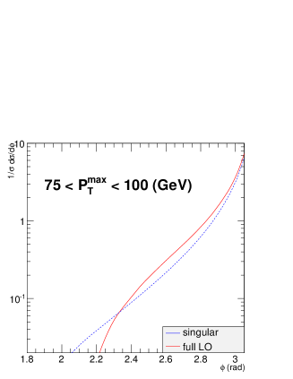
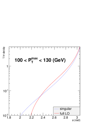
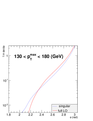
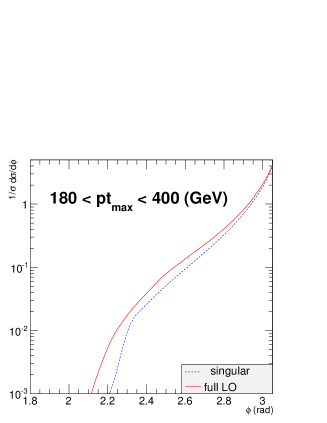
Figure 6: The comparisons between the asymptotic derivations of Eq. (101) and the full LO calculations for the kinematics specified by the D0 collaboration at the Tevatron. The LO curves come from Ref. Abazov:2004hm .

In Fig. 6, we compare the above differential cross section, for dijet production at the Tevatron for the kinematics specified by the D0 Collaboration Abazov:2004hm , to the fixed order perturbative calculation with one gluon radiation contributions. From these plots, we can see that the above asymptotic results capture the leading contributions at low transverse momentum where $\phi$ is close to $\pi$ for the back-to-back azimuthal correlation region. We would like to emphasize that the jet size dependent terms are crucial to make these comparisons. Without them, the agreements between the full LO calculations and our asymptotic derivation results will not be as evident as shown in Fig. 6.

VI Factorization and Resummation

Clearly, from the derivations in the last section, and the plots of the differential cross sections shown in Fig. 6, we see that the collinear factorization calculations for the dijet production lead to divergent behavior at low imbalance transverse momentum $q_{\perp}$, which corresponds to the back-to-back azimuthal angular correlation between the two final state jets. In this region, to have a reliable prediction, we need to perform the resummation. Since we are interested in the dependence of the differential cross sections on the transverse momentum $q_{\perp}$, the TMD resummation is the appropriate framework for carrying out our theory calculations.

The TMD resummation was originally derived for Drell-Yan type of hard processes, where the final state only contains color neutral particle with large invariant mass. In order to apply this resummation formalism to the current case of dijet production in hadronic collisions, some modifications are needed. In particular, the two final state jets carry color so that additional soft gluon radiation will introduce large logarithms associated with the final state jets. Although, these additional interactions will not modify the leading double logarithmic contribution, they will enter at the next-to-leading logarithmic level. This is evident from the explicit calculations discussed in the previous section.

To carry out the TMD factorization, we extend the original CSS formalism, and take into account the final state radiation by assuming a soft factor in the factorization formalism. The exact same idea has been applied to resum large logarithms associated with the threshold logarithms for dijet productions. The similarity between the TMD and threshold resummation is not surprising, because they both deal with soft and collinear gluon radiations.

In this section, we will argue the TMD factorization for dijet production based on the explicit one-loop calculations presented in the previous sections. The factorization is verified in the transverse momentum space and $b_{\perp}$-space at the one-loop order. At this order, we have to take into account the matrix form of the hard and soft factors. The explicit comparisons support the factorization we argued in this paper.

With the explicit form of the TMD factorization formulas, we derive the resummation result by solving the relevant renormalization group equations. In particular, the TMDs follow the examples of color neutral particle productions, which have studied extensively in the literature. The additional soft factor obeys the renormalization group equation controlled by the anomalous dimension. We calculate the soft factor at one-loop order, from which we derive the anomalous dimension at one-loop order. Solving this renormalization group equation, we resume the sub-leading logarithms in dijet production processes.

Generically, the low transverse momentum $q_{\perp}$ originates from collinear gluon radiation associated with the incoming partons and the soft gluon radiation effects. In particular, the collinear gluon radiation from the incoming partons contribute to the total transverse momentum of the final state particles. This is the dominant contribution in dijet production in hadronic collisions. The collinear gluon radiation associated with the two final state jets will not contribute to the total transverse momentum of the dijet. This is because they are factorized into the jet contribution which do not contribute a finite $q_{\perp}$ as we have shown in Sec. III. On the other hand, soft gluon radiation among the incoming partons and final state jets will contribute to the low imbalance transverse momentum of the dijet. To account for this part of contribution, we introduce the soft factor in the TMD factorization. Since the final states carry color, the soft gluon radiation is more complicated than that for the color neutral particle production in hadronic collisions.

We follow the method developed for threshold resummation in dijet productions in hadronic collisions in Ref. Kidonakis:1997gm , where the soft factor is formulated in the orthogonal color space and both the incoming and outgoing partons are represented by Eikonal gauge links. Because of light-cone singularity in the parton distributions, we choose off-light-front gauge links for the incoming partons. Meanwhile, the Wilson lines associated with the final state jets are constructed in such a way that only out-of-cone gluon radiation contribute to a nonzero $q_{\perp}$. Consequently, the soft factor in our calculations will depend on the jet cone size .

Following the above argument, we can write down the factorization formula as,

$$\frac{d^{4}\sigma}{dy_{1}dy_{2}dP_{T}^{2}d^{2}q_{\perp}} = \sum\limits_{ab}\sigma_{0}\int d^{2}k_{1\perp}d^{2}k_{2\perp}d^{2}\lambda_{\perp}\,x_{a}f_{a}(x_{a},k_{1\perp})\,x_{b}f_{b}(x_{b},k_{2\perp})$$ (102)

$$\times\textmd{Tr}\left[\mathbf{H}_{ab\to cd}(Q^{2})\mathbf{S}_{ab\to cd}(\lambda_{\perp})\right]\delta^{(2)}(\vec{k}_{1\perp}+\vec{k}_{2\perp}+\lambda_{\perp}-\vec{q}_{\perp})\;,$$

where $f_{a}(x_{1},k_{1\perp})$ and $f_{b}(x_{2},k_{2\perp})$ are TMDs and will be introduced in the following. Here, the hard factor and soft factor are expressed in the matrix forms in the color spaces for the incoming and outgoing partons. We can also express $W(b_{\perp})$ in the $b_{\perp}$-space as

$$W_{ab\to cd} = x_{1}\,f_{a}(x_{1},b_{\perp},\zeta_{1}^{2},\mu^{2},\rho^{2})x_{2}\,f_{b}(x_{2},b_{\perp},\zeta_{2}^{2},\mu^{2},\rho^{2})$$ (103)

$$\times \textmd{Tr}\left[\mathbf{H}_{ab\to cd}(Q^{2},\mu^{2},\rho^{2},y_{1}-y_{2},R_{1},R_{2})\mathbf{S}_{ab\to cd}(b_{\perp},\mu^{2},\rho^{2},y_{1}-y_{2},R_{1},R_{2})\right]\ ,$$

where we have shown all the explicit dependence of the TMDs and hard and soft factors.

In the following, we will first introduce the TMDs, and then formulate the soft factors for all partonic channels. With these factors calculated in perturbation theory, we will show the above factorization is valid at one-loop order, by comparing to the derivations in the last few sections.

VI.1 Transverse Momentum Dependent Parton Distributions

In the factorization formula, $xf_{i}(x,b_{\perp},\zeta^{2},\mu^{2})$ is the Fourier transformation of quark TMD parton distribution $xf_{i}(x,k_{\perp},\zeta^{2},\mu^{2})$. We follow the Ji-Ma-Yuan scheme Ji:2004wu to define the TMDs. For the quark distribution, we have 

$$xf_{q}(x,k_{\perp},\zeta^{2},\mu^{2}) = \int\frac{d\xi^{-}d^{2}\xi_{\perp}}{P^{+}(2\pi)^{3}}e^{-ixP^{+}\xi^{-}+i\vec{k}_{\perp}\cdot\vec{\xi}_{\perp}}$$ (104)

$$~{}~{}\times\frac{\left\langle P|\Psi(\xi^{-},\xi_{\perp}){\cal L}^{\dagger}_{v}(\xi^{-},\xi_{\perp})\gamma^{+}{\cal L}_{v}(0,0_{\perp})\Psi(0)|P\right\rangle}{\langle 0|{\cal L}_{\bar{v}cb^{\prime}}^{\dagger}(b_{\perp};\infty){\cal L}_{vb^{\prime}a}^{\dagger}(\infty;b_{\perp}){\cal L}_{vab}(0;\infty){\cal L}_{\bar{v}bc}(\infty;0)|0\rangle}\ .$$

For gluon one, it can be written as:

$$xf_{g}(x,k_{\perp},\zeta^{2},\mu^{2}) = \int\frac{d\xi^{-}d^{2}\xi_{\perp}}{P^{+}(2\pi)^{3}}e^{-ixP^{+}\xi^{-}+i\vec{k}_{\perp}\cdot\vec{\xi}_{\perp}}$$ (105)

$$~{}~{}\times\frac{\left\langle P|F^{+}_{a\mu}(\xi^{-},\xi_{\perp}){\cal L}^{\dagger}_{vab}(\xi^{-},\xi_{\perp})\gamma^{+}{\cal L}_{vbc}(0,0_{\perp})F_{c}^{\mu+}(0)|P\right\rangle}{\langle 0|{\cal L}_{\bar{v}cb^{\prime}}^{\dagger}(b_{\perp};\infty){\cal L}_{vb^{\prime}a}^{\dagger}(\infty;b_{\perp}){\cal L}_{vab}(0;\infty){\cal L}_{\bar{v}bc}(\infty;0)|0\rangle}\ .$$

In the above equations, the relevant gauge links have to apply, in the fundamental and adjoint representations for the quark and gluon distributions, respectively. The gauge link ${\cal L}_{v}$ is chosen along the direction $v$,

$${\cal L}_{v}(\xi^{-},\xi_{\perp})=Pexp\left(-ig\int_{-\infty}^{0}d\lambda v\cdot A(\lambda v+\xi)\right)\ ,$$ (106)

for both cases, in the appropriate representations of $SU(3)$, adjoint for the gluon distribution and fundamental for the quark distribution, respectively. Similarly, we define the TMDs from hadron $\bar{P}$, which depend on the gauge link along the direction $\bar{v}$. The vectors $v$ and $\bar{v}$ are off-light-front: $v=(v^{+},v^{-},0_{\perp})$ with $v^{-}\gg v^{+}$ and $\bar{v}=(\bar{v}^{+},\bar{v}^{-},0_{\perp})$ with $\bar{v}^{-}\ll\bar{v}^{+}$, and . Since non-light-like vectors exist, the TMD parton distribution depends on a new large scale $\zeta^{2}=(2v\cdot P)/v^{2}$ and a free parameter $\rho^{2}=\frac{v^{-}\bar{v}^{+}}{\bar{v}^{-}v^{+}}$. Based on these definitions, we can calculate them under perturbative QCD order by order, and can be expressed in terms of the integrated parton distributions. At one-loop order, the gluon distribution can be written as Ji:2004wu :

$$f_{g}(x,b,\zeta,\mu,\rho) = \frac{\alpha_{s}C_{A}}{2\pi}\int\frac{dx^{\prime}}{x^{\prime}}\left\{\ln\frac{b_{0}^{2}}{\bar{\mu}^{2}b^{2}}\left[{\cal P}_{gg}(\xi)f_{g}(x^{\prime},\bar{\mu})+{\cal P}_{gq}(\xi)f_{q}(x^{\prime},\bar{\mu})\right]+\delta(\xi-1)f_{g}(x,\bar{\mu})\right.$$ (107)

$$\left.\times\left[\left(\ln\rho^{2}+2\beta_{0}-1\right)\ln\frac{b^{2}\mu^{2}}{b_{0}^{2}}e^{2\gamma_{E}}-\frac{1}{2}\ln^{2}\frac{b^{2}\zeta^{2}}{b_{0}^{2}}\right.\right.\left.\left.+\frac{3}{2}\ln\frac{\zeta^{2}}{\mu^{2}}-\frac{\pi^{2}}{2}-\frac{7}{2}\right]\right\}\ ,$$

where $\xi=x/x^{\prime}$. For the quark distribution,

$$f_{q}(x,b,\zeta,\mu,\rho) = \frac{\alpha_{s}C_{F}}{2\pi}\int\frac{dx^{\prime}}{x^{\prime}}\left\{\ln\frac{b_{0}^{2}}{\bar{\mu}^{2}b^{2}}\left[{\cal P}_{qg}(\xi)f_{g}(x^{\prime},\bar{\mu})+{\cal P}_{qq}(\xi)f_{q}(x^{\prime},\bar{\mu})\right]+\delta(\xi-1)f_{q}(x,\bar{\mu})\right.$$ (108)

$$\left.\times\left[\left(\ln\rho^{2}-\frac{1}{2}\right)\ln\frac{b^{2}\mu^{2}}{b_{0}^{2}}-\frac{1}{2}\ln^{2}\frac{b^{2}\zeta^{2}}{b_{0}}\right.\right.\left.\left.-\frac{\pi^{2}}{4}-1\right]\right\}\ .$$

In the above equations, ${\cal P}_{ij}$ are splitting kernels. At one-loop order, we have

$${\cal P}_{gg}(x) = 6\left(\frac{1-x}{x}+\frac{x}{(1-x)_{+}}+x(1-x)+\beta_{0}\delta(1-x)\right)\ ,$$ (109)

$${\cal P}_{gq}(x) = \frac{4}{3}\left(\frac{1+(1-x)^{2}}{x}\right)\ ,$$ (110)

$${\cal P}_{qq}(x) = \frac{4}{3}\left(\frac{1+x^{2}}{(1-x)_{+}}+\frac{3}{2}\delta(1-x)\right)\ ,$$ (111)

$${\cal P}_{qg}(x) = \frac{1}{2}\left(x^{2}+(1-x)^{2}\right)\ .$$ (112)

Similarly, we can obtain the $k_{\perp}$-dependent expressions for the TMDs from these references.

VI.2 Color Space Decompositions for the Soft and Hard Factors

It has been shown in Refs. Kidonakis:1997gm , for soft gluon radiation in dijet production, it is more convenient to construct the factorization in the color space matrix, where the soft and hard factors can be calculated in the orthogonal color bases. In particular, the associated anomalous dimension for the soft factors can be formulated and the relevant resummation can be performed accordingly.

In this paper, we consider dijet production through the partonic $2\to 2$ subprocesses. Therefore, for each partonic channel, we will construct the color-space bases depending on the color indexes of two incoming partons and two outgoing partons. The soft gluon radiation does not modify the fundamental scattering structure for each partonic channel, so that the color-space bases are constructed for all order perturbative calculations. In addition, the color-space bases are not unique. In our calculations, we follow those used in Ref. Kidonakis:1997gm . For the quark-quark scattering subprocesses, we have fundamental representation from both incoming and outgoing partons, for example,

$$q^{k}_{a}+\bar{q}^{k}_{b}\rightarrow q^{k}_{c}+\bar{q}^{k}_{d},\;\;\;q^{k}_{a}+\bar{q}^{k}_{b}\rightarrow q^{j}_{c}+\bar{q}^{j}_{d},\;\;\;q^{j}_{a}+\bar{q}^{k}_{b}\rightarrow q^{j}_{c}+\bar{q}^{k}_{d}\ ,$$ (113)

where $j$ and $k$ indicate the flavors of the quarks, and $a,b,c$ and $d$ are the color indices. For this channel, we have two independent color configurations,

$$C^{ab}_{1cd}=\delta_{ac}\delta_{bd}\ ,\;\;\;\;C^{ab}_{2cd}=T^{a^{\prime}}_{ac}T^{a^{\prime}}_{bd}\ ,$$ (114)

corresponding to the color-singlet and the color-octet couplings, respectively. Similarly, we have the same decomposition for identical quark-quark scattering subprocess,

$$q^{k}_{a}+q^{k}_{b}\rightarrow q^{k}_{c}+q^{k}_{d},\;\;\;q^{j}_{a}+q^{k}_{b}\rightarrow q^{j}_{c}+q^{k}_{d}\ .$$ (115)

For $gg\to q\bar{q}$ channel,

$$g_{a}+g_{b}\rightarrow\bar{q}^{k}_{c}+q^{k}_{d},$$ (116)

we have three independent color bases,

$$C^{ab}_{1cd}=T^{a^{\prime}}_{ac}T^{a^{\prime}}_{cd}\ ,\;\;\;\;C^{ab}_{2cd}=d^{abc^{\prime}}T^{c^{\prime}}_{cd}\ ,\;\;\;\;C^{ab}_{3cd}=if^{abc^{\prime}}T^{c^{\prime}}_{cd}\ .$$ (117)

Similarly for $q\bar{q}\to gg$ channel:

$$\bar{q}^{k}_{c}+q^{k}_{d}\rightarrow g_{a}+g_{b},\ ,$$ (118)

we have

$$C^{cd}_{1ab}=T^{a^{\prime}}_{ac}T^{a^{\prime}}_{cd}\ ,\;\;\;\;C^{cd}_{2ab}=d^{abc^{\prime}}T^{c^{\prime}}_{cd}\ ,\;\;\;\;C^{cd}_{3ab}=if^{abc^{\prime}}T^{c^{\prime}}_{cd}\ .$$ (119)

That will also apply to $qg\to qg$ channel,

$$q^{k}_{c}+g_{a}\rightarrow q^{k}_{d}+g_{b}\ ,$$ (120)

where we have

$$C^{ac}_{1bd}=T^{a^{\prime}}_{ac}T^{a^{\prime}}_{cd}\ ,\;\;\;\;C^{ac}_{2bd}=d^{abc^{\prime}}T^{c^{\prime}}_{cd}\ ,\;\;\;\;C^{ac}_{3bd}=if^{abc^{\prime}}T^{c^{\prime}}_{cd}\ .$$ (121)

For $gg\to gg$ channel,

$$g_{a}+g_{b}\rightarrow g_{c}+g_{d}\ ,$$ (122)

however, it is much more complicated,

$$C^{ab}_{1cd} = \frac{i}{4}(f^{abc^{\prime}}d^{cdc^{\prime}}-d^{abc^{\prime}}f^{cdc^{\prime}})\ ,\;\;\;\;C^{ab}_{2cd}=\frac{i}{4}(f^{abc^{\prime}}d^{cdc^{\prime}}+d^{abc^{\prime}}f^{cdc^{\prime}})\ ,$$

$$C^{ab}_{3cd} = \frac{i}{4}(f^{acc^{\prime}}d^{bdc^{\prime}}+d^{acc^{\prime}}f^{bdc^{\prime}})\ ,\;\;\;\;C^{ab}_{4cd}=\frac{1}{8}\delta^{ac}\delta^{bd}\ ,$$

$$C^{ab}_{5cd} = \frac{3}{5}d^{acc^{\prime}}d^{bdc^{\prime}}\ ,\;\;\;\;C^{ab}_{6cd}=\frac{1}{3}f^{acc^{\prime}}f^{bdc^{\prime}}\ ,$$

$$C^{ab}_{7cd} = \frac{1}{2}(\delta^{ab}\delta^{cd}-\delta^{ad}\delta^{bc})-\frac{1}{3}f^{acc^{\prime}}f^{bdc^{\prime}}\ ,$$

$$C^{ab}_{8cd} = \frac{1}{2}(\delta^{ab}\delta^{cd}+\delta^{ad}\delta^{bc})-\frac{1}{8}\delta^{ac}\delta^{bd}-\frac{3}{5}d^{acc^{\prime}}d^{bdc^{\prime}}\ ,$$ (123)

where we have eight independent color bases.

With the above color bases, we can decompose the soft factors in the matrix form. The associated soft gluon radiation is represented by eight gauge links. This is because all the initial and final state can radiate or absorb soft gluons. Therefore, we can decompose the soft factor, according to the following formula,

$$S_{IJ}(b_{\perp}) = \int_{0}^{\pi}\frac{(\sin\phi)^{-2\epsilon}d\phi}{\frac{\sqrt{\pi}\Gamma(\frac{1}{2}-\epsilon)}{\Gamma(1-\epsilon)}}\;C^{bb^{\prime}}_{Iii^{\prime}}C^{aa^{\prime}}_{Jll^{\prime}}\langle 0|{\cal L}_{vcb^{\prime}}^{\dagger}(b_{\perp}){\cal L}_{\bar{v}bc^{\prime}}(b_{\perp}){\cal L}_{\bar{v}c^{\prime}a^{\prime}}^{\dagger}(0){\cal L}_{vac}(0)$$ (124)

$$\times{\cal L}_{nji}^{\dagger}(b_{\perp}){\cal L}_{\bar{n}i^{\prime}k}(b_{\perp}){\cal L}_{\bar{n}kl}^{\dagger}(0){\cal L}_{nl^{\prime}j}(0)|0\rangle\ ,$$

where $IJ$ represent the color indices in the color-space bases constructed above. Therefore, $S_{IJ}$ is the matrix element in the associated color-space bases for a particular partonic channel. As mentioned above, we have four gauge links associated with two incoming partons, for which we follow the TMDs to adopt off-light-cone vectors $v$ and $\bar{v}$ to construct the gauge links. The off-light-cone vectors are applied to regulate the light-cone singularities. For the two outgoing partons, we apply the off-shellness to cast the out-of-cone radiation contribution to the soft factor. This regulation depends on the jet size. That is why we introduce the off-shellness $n^{2}=R_{1}^{2}P_{T}^{2}/Q^{2}$ and $\bar{n}^{2}=R_{2}^{2}P_{T}^{2}/Q^{2}$ for the two final state jets with jet size $R_{1}$ and $R_{2}$, respectively. $C^{bb^{\prime}}_{Iii^{\prime}}$ and $C^{aa^{\prime}}_{Jll^{\prime}}$ represent the corresponding color configurations, as introduced above.

It is straightforward to calculate the soft factor at the leading Born order, $S_{IJ}=C_{Iii^{\prime}}^{aa^{\prime}}C_{Ji^{\prime}i}^{a^{\prime}a}$. For the channels in Eqs. (115,113), we find

$$S^{(0)}=\left[\begin{array}[]{cc}C_{A}^{2}&0\\ 0&\frac{C_{A}C_{F}}{2}\\ \end{array}\right]\ .$$ (127)

For the channels in Eqs. (116,118,120), we have

$$S^{(0)}=\left[\begin{array}[]{ccc}2C_{A}^{2}C_{F}&0&0\\ \\ 0&(C_{A}^{2}-4)C_{F}&0\\ \\ 0&0&C_{A}^{2}C_{F}\\ \end{array}\right]\ .$$ (133)

For the channels in Eq. (122), we obtain

$$S^{(0)}=\left[\begin{array}[]{cccccccc}5&0&0&0&0&0&0&0\\ 0&5&0&0&0&0&0&0\\ 0&0&5&0&0&0&0&0\\ 0&0&0&1&0&0&0&0\\ 0&0&0&0&8&0&0&0\\ 0&0&0&0&0&8&0&0\\ 0&0&0&0&0&0&20&0\\ 0&0&0&0&0&0&0&27\\ \end{array}\right]\ .$$ (142)

The hard factor ${\bf H}$ should be expanded by the same color bases. At the tree level, our results are consistent with those in Ref. Kidonakis:1997gm . For completeness, we list these results in the following. For the partonic channel of $q^{k}+\bar{q}^{k}\rightarrow q^{k}+\bar{q}^{k}$,

$$H^{(0)}=\left[\begin{array}[]{cc}H_{11}&H_{12}\\ H_{21}&H_{22}\\ \end{array}\right]\ ,$$ (145)

where

$$H_{11} = \frac{2C_{F}^{2}}{C_{A}^{4}}\frac{t^{2}+u^{2}}{s^{2}}\ ,$$

$$H_{12} = H_{21}=-\frac{2C_{F}}{C_{A}^{4}}\frac{t^{2}+u^{2}}{s^{2}}+\frac{2C_{F}}{C_{A}^{3}}\frac{u^{2}}{st}\ ,$$

$$H_{22} = \frac{2}{C_{A}^{4}}\frac{t^{2}+u^{2}}{s^{2}}+\frac{4}{C_{A}^{2}}\frac{s^{2}+u^{2}}{t^{2}}-\frac{4}{C_{A}^{3}}\frac{u^{2}}{st}\ .$$ (146)

Similarly, the partonic channel $q^{k}+\bar{q}^{k}\rightarrow q^{j}+\bar{q}^{j}$ is expressed in the $2\times 2$ matrix with

$$H_{11} = \frac{2C_{F}^{2}}{C_{A}^{4}}\frac{t^{2}+u^{2}}{s^{2}}$$

$$H_{12} = H_{21}=-\frac{2C_{F}}{C_{A}^{4}}\frac{t^{2}+u^{2}}{s^{2}}$$

$$H_{22} = \frac{2}{C_{A}^{4}}\frac{t^{2}+u^{2}}{s^{2}}\ .$$ (147)

And for channel $q^{k}+\bar{q}^{j}\rightarrow q^{k}+\bar{q}^{j}$,

$$H_{11} = H_{12}=H_{21}=0\ ,$$

$$H_{22} = \frac{2}{C_{A}^{2}}\frac{s^{2}+u^{2}}{t^{2}}\ .$$ (148)

For channel $q^{k}+q^{k}\rightarrow q^{k}+q^{k}$,

$$H_{11} = \frac{2C_{F}^{2}}{C_{A}^{4}}\frac{t^{2}+s^{2}}{u^{2}}\ ,$$

$$H_{12} = H_{21}=-\frac{2C_{F}}{C_{A}^{4}}\frac{t^{2}+s^{2}}{u^{2}}+\frac{2C_{F}}{C_{A}^{3}}\frac{s^{2}}{ut}\ ,$$

$$H_{22} = \frac{2}{C_{A}^{2}}\frac{s^{2}+u^{2}}{t^{2}}+\frac{2}{C_{A}^{4}}\frac{s^{2}+t^{2}}{u^{2}}-\frac{2}{C_{A}}\frac{s^{2}}{ut}\ .$$ (149)

For channel $q^{k}+q^{j}\rightarrow q^{k}+q^{j}$,

$$H_{11} = H_{12}=H_{21}=0\ ,$$

$$H_{22} = \frac{2}{C_{A}^{2}}\frac{s^{2}+u^{2}}{t^{2}}\ .$$ (150)

For channel $g+g\rightarrow q+\bar{q}$ and $q+\bar{q}\rightarrow g+g$, the hard factor is calculated as $3\times 3$ matrix,

$$H^{(0)}=\left[\begin{array}[]{ccc}H_{11}&H_{12}&H_{13}\\ H_{21}&H_{22}&H_{23}\\ H_{31}&H_{32}&H_{33}\\ \end{array}\right]\ ,$$ (154)

where

$$H_{11} = \frac{1}{2C_{A}^{4}}\frac{u^{2}+t^{2}}{ut}\ ,$$

$$H_{12} = H_{21}=\frac{1}{2C_{A}^{3}}\frac{u^{2}+t^{2}}{ut}\ ,$$

$$H_{22} = \frac{1}{2C_{A}^{2}}\frac{u^{2}+t^{2}}{ut}\ ,$$

$$H_{13} = H_{31}=\frac{1}{2C_{A}^{3}}\frac{t^{2}-u^{2}}{ut}+\frac{1}{C_{A}^{3}}\frac{t-u}{s}\ ,$$

$$H_{23} = H_{32}=\frac{1}{2C_{A}^{2}}\frac{t^{2}-u^{2}}{ut}+\frac{1}{C_{A}^{2}}\frac{t-u}{s}\ ,$$

$$H_{33} = \frac{1}{2C_{A}^{2}}\frac{s^{2}}{ut}+\frac{4}{C_{A}^{2}}\frac{tu}{s^{2}}-\frac{3}{C_{A}^{2}}\ .$$ (155)

For channel $q+g\rightarrow q+g$, we find a similar $3\times 3$ matrix with

$$H_{11} = \frac{1}{4C_{A}^{4}C_{F}}\frac{t^{2}-2su}{su}\ ,$$

$$H_{12} = H_{21}=\frac{1}{4C_{A}^{3}C_{F}}\frac{t^{2}-2su}{su}\ ,$$

$$H_{22} = \frac{1}{4C_{A}^{2}C_{F}}\frac{t^{2}-2su}{su}\ ,$$

$$H_{13} = H_{31}=-\frac{1}{2C_{A}^{3}C_{F}}\frac{s^{2}t+4s^{2}u+2stu-tu^{2}}{stu}\ ,$$

$$H_{23} = H_{32}=-\frac{1}{2C_{A}^{2}C_{F}}\frac{s^{2}t+4s^{2}u+2stu-tu^{2}}{stu}\ ,$$

$$H_{33} = \frac{1}{4C_{A}^{2}C_{F}}\frac{(2su-t^{2})(t^{2}-4su)}{st^{2}u}\ .$$ (156)

For channel $g+g\rightarrow g+g$, however, we have $8\times 8$ matrix,

$$H^{(0)}=\left[\begin{array}[]{cccccccc}0&0&0&0&0&0&0&0\\ 0&0&0&0&0&0&0&0\\ 0&0&0&0&0&0&0&0\\ 0&0&0&H_{44}&H_{45}&H_{46}&0&H_{48}\\ 0&0&0&H_{54}&H_{55}&H_{56}&0&H_{58}\\ 0&0&0&H_{64}&H_{65}&H_{66}&0&H_{68}\\ 0&0&0&0&0&0&0&0\\ 0&0&0&H_{84}&H_{85}&H_{86}&0&H_{88}\\ \end{array}\right]\ ,$$ (165)

where

$$H_{44} = -\frac{9}{16}\frac{(s^{2}-tu)(st-u^{2})}{s^{2}u^{2}}\ ,$$

$$H_{45} = H_{54}=-\frac{9}{32}\frac{(s^{2}-tu)(st-u^{2})}{s^{2}u^{2}}\ ,$$

$$H_{55} = -\frac{9}{64}\frac{(s^{2}-tu)(st-u^{2})}{s^{2}u^{2}}\ ,$$

$$H_{46} = H_{64}=-\frac{9}{32}\frac{(s-u)\left(s^{2}+su+u^{2}\right)\left(su-t^{2}\right)}{s^{2}tu^{2}}\ ,$$

$$H_{56} = H_{65}=-\frac{9}{64}\frac{(s-u)\left(s^{2}+su+u^{2}\right)\left(su-t^{2}\right)}{s^{2}tu^{2}}\ ,$$

$$H_{66} = \frac{9\left(s^{2}t-2su^{2}+t^{2}u\right)\left(2s^{2}u-st^{2}-tu^{2}\right)}{64s^{2}t^{2}u^{2}}\ ,$$

$$H_{48} = H_{84}=\frac{3}{16}\frac{(s^{2}-tu)(st-u^{2})}{s^{2}u^{2}}\ ,$$

$$H_{58} = H_{85}=\frac{3}{32}\frac{(s^{2}-tu)(st-u^{2})}{s^{2}u^{2}}\ ,$$

$$H_{68} = H_{86}=-\frac{3}{32}\frac{(s-u)\left(s^{2}+su+u^{2}\right)\left(su-t^{2}\right)}{s^{2}tu^{2}}\ ,$$

$$H_{88} = -\frac{1}{16}\frac{(s^{2}-tu)(st-u^{2})}{s^{2}u^{2}}\ .$$ (166)

The above hard factors are normalized to reproduce the leading order differential cross sections in Sec. II,

$$h_{12\to 34}^{(0)}=S_{IJ}^{12\to 34(0)}H_{JI}^{12\to 34(0)}\ ,$$ (167)

where sum over $IJ$ is understood. Because the leading order soft factor is diagonalized, it is simple to verify the above equation.

VI.3 Soft Factor and the Anomalous Dimension at One-loop order

Figure 7: Representative diagrams contributing to the soft function at the NLO.

At one-loop order, we will expand the soft factor definition with perturbative corrections. The gluon radiations between all gauge links will contribute. For convenience we separate out the common kinematic integrals from the color factors for each soft factor calculation,

$$S^{(1)}=\sum\limits_{ij}W_{ij}I_{ij}\ ,$$ (168)

where $ij$ label the associated gauge links: $12$ for the incoming two partons and $34$ for the outgoing partons. In the above equation, $I_{ij}$ represent the kinematic integrals for the soft gluon radiation between $i$ and $j$ gauge links, whereas the factor $W_{ij}$ represent the associated color factor in the matrix form for particular partonic channel.

We show in Fig. (7)  a few representative real gluon emission diagrams, labelled by the relevant kinematic integral $I_{ij}$, which contribute to the soft function at the next-to-leading order (NLO) in $\alpha_{s}$.

For the $I_{34}$ diagram, with gluon connecting $3$ and $4$ gauge links, we find the following results:

$$I_{34}(k_{t}) = \frac{\alpha_{s}}{2\pi^{2}}\int^{\pi}_{0}\frac{(\sin\phi)^{-2\epsilon}d\phi}{\frac{\sqrt{\pi}\Gamma(\frac{1}{2}-\epsilon)}{\Gamma(1-\epsilon)}}\int dk^{+}dk^{-}\frac{2n_{j}\cdot\bar{n}_{j}}{(k\cdot n_{j})(k\cdot\bar{n}_{j})}\delta(k^{2})\theta(k_{0})$$

$$= \frac{\alpha_{s}}{2\pi^{2}}\;\frac{1}{k_{t}^{2}}\left[\ln\left(\frac{Q^{4}}{R_{1}^{2}R_{2}^{2}P_{T}^{4}}\right)+\epsilon\left(\frac{1}{2}\ln^{2}\frac{1}{R_{1}^{2}}+\frac{1}{2}\ln^{2}\frac{1}{R_{2}^{2}}+\frac{\pi^{2}}{3}-4\ln\frac{s}{-t}\ln\frac{s}{-u}\right)\right]\ ,$$

in the transverse momentum space, where $k$ represents the radiated gluon momentum. We have kept the $\epsilon$ term in the above equation, because they will contribute to a finite term when Fourier transforming to $b_{\perp}$-space. In the calculations, $n_{j}$ and $\bar{n}_{j}$ carry the momentum direction of two outgoing jets, and therefore, the scalar product $n_{j}\cdot\bar{n}_{j}$ enters in the final result which is proportional to $Q^{2}/P_{\perp}^{2}$. That is the cause of having the logarithmic dependence on this factor in our final result. Again, the offshellness of the two outgoing gauge links are introduced to cast the contribution that is only associated with out-of-cone radiation. Gluon radiation within the jet cone will not induce a nonzero transverse momentum of the dijet and its contribution needs to be subtracted out.

Similarly, for gluon connection between all other gauge links needed in the final calculations, we find

$$I_{13}(k_{t}) = 2\frac{\alpha_{s}}{2\pi^{2}}\int^{\pi}_{0}\frac{(\sin\phi)^{-2\epsilon}d\phi}{\frac{\sqrt{\pi}\Gamma(\frac{1}{2}-\epsilon)}{\Gamma(1-\epsilon)}}\int dk^{+}dk^{-}\frac{\bar{v}\cdot n_{j}}{(k\cdot n_{j})(k\cdot\bar{v})}\delta(k^{2})\theta(k_{0})$$ (170)

$$= \frac{\alpha_{s}}{2\pi^{2}}\frac{1}{k_{t}^{2}}\left[\ln{\left(\frac{t^{2}\rho^{2}}{\zeta_{1}^{2}\;P_{T}^{2}R_{1}^{2}}\right)}+\epsilon\left(\frac{1}{2}\ln^{2}\frac{1}{R_{1}^{2}}+\frac{\pi^{2}}{6}\right)\right]\ ,$$

$$I_{14}(k_{t}) = 2\frac{\alpha_{s}}{2\pi^{2}}\int^{\pi}_{0}\frac{(\sin\phi)^{-2\epsilon}d\phi}{\frac{\sqrt{\pi}\Gamma(\frac{1}{2}-\epsilon)}{\Gamma(1-\epsilon)}}\int dk^{+}dk^{-}\frac{\bar{v}\cdot\bar{n}_{j}}{(k\cdot\bar{n}_{j})(k\cdot\bar{v})}\delta(k^{2})\theta(k_{0})$$ (171)

$$= \frac{\alpha_{s}}{2\pi^{2}}\frac{1}{k_{t}^{2}}\left[\ln{\left(\frac{u^{2}\rho^{2}}{\zeta_{1}^{2}\;P_{T}^{2}R_{2}^{2}}\right)}+\epsilon\left(\frac{1}{2}\ln^{2}\frac{1}{R_{2}^{2}}+\frac{\pi^{2}}{6}\right)\right]\ ,$$

$$I_{24}(k_{t}) = 2\frac{\alpha_{s}}{2\pi^{2}}\int^{\pi}_{0}\frac{(\sin\phi)^{-2\epsilon}d\phi}{\frac{\sqrt{\pi}\Gamma(\frac{1}{2}-\epsilon)}{\Gamma(1-\epsilon)}}\int dk^{+}dk^{-}\frac{v\cdot n_{j}}{(k\cdot n_{j})(k\cdot v)}\delta(k^{2})\theta(k_{0})$$ (172)

$$= \frac{\alpha_{s}}{2\pi^{2}}\frac{1}{k_{t}^{2}}\left[\ln{\left(\frac{t^{2}\rho^{2}}{\zeta_{2}^{2}\;P_{T}^{2}R_{2}^{2}}\right)}+\epsilon\left(\frac{1}{2}\ln^{2}\frac{1}{R_{2}^{2}}+\frac{\pi^{2}}{6}\right)\right]\ ,$$

$$I_{23}(k_{t}) = 2\frac{\alpha_{s}}{2\pi^{2}}\int^{\pi}_{0}\frac{(\sin\phi)^{-2\epsilon}d\phi}{\frac{\sqrt{\pi}\Gamma(\frac{1}{2}-\epsilon)}{\Gamma(1-\epsilon)}}dk^{+}dk^{-}\frac{v\cdot\bar{n}_{j}}{(k\cdot\bar{n}_{j})(k\cdot v)}\delta(k^{2})\theta(k_{0})$$ (173)

$$= \frac{\alpha_{s}}{2\pi^{2}}\frac{1}{k_{t}^{2}}\left[\ln{\left(\frac{u^{2}\rho^{2}}{\zeta_{2}^{2}\;P_{T}^{2}R_{1}^{2}}\right)}+\epsilon\left(\frac{1}{2}\ln^{2}\frac{1}{R_{1}^{2}}+\frac{\pi^{2}}{6}\right)\right]\ ,$$

$$I_{11}(k_{t}) = I_{22}(k_{t})=-\frac{\alpha_{s}}{2\pi^{2}}\int^{\pi}_{0}\frac{(\sin\phi)^{-2\epsilon}d\phi}{\frac{\sqrt{\pi}\Gamma(\frac{1}{2}-\epsilon)}{\Gamma(1-\epsilon)}}\int dk^{+}dk^{-}\frac{\bar{v}\cdot\bar{v}}{(k\cdot\bar{v})^{2}}\delta(k^{2})\theta(k_{0})$$ (174)

$$= -\frac{\alpha_{s}}{2\pi^{2}}\frac{1}{k_{t}^{2}}\ ,$$

$$I_{12}(k_{t}) = 2\frac{\alpha_{s}}{2\pi^{2}}\int^{\pi}_{0}\frac{(\sin\phi)^{-2\epsilon}d\phi}{\frac{\sqrt{\pi}\Gamma(\frac{1}{2}-\epsilon)}{\Gamma(1-\epsilon)}}\int dk^{+}dk^{-}\frac{\bar{v}\cdot v}{(k\cdot\bar{v})(k\cdot v)}\delta(k^{2})\theta(k_{0})$$ (175)

$$= \frac{\alpha_{s}}{2\pi^{2}}\frac{1}{k_{t}^{2}}\ln\rho^{2}\ .$$

Here, we did not list either $I_{33}$ or $I_{44}$, because they will not contribute to the soft factor.

For the contribution from virtual diagrams, all the integrals are proportional to

$$\frac{1}{\epsilon_{IR}}-\frac{1}{\epsilon_{UV}}\ .$$ (176)

After introducing the UV counter-terms which are proportional to

$$-\frac{1}{\epsilon_{UV}}+\gamma_{E}+\ln\frac{1}{4\pi}\ ,$$ (177)

only IR divergence will be left and cancel the singularity in real diagrams, after we have performed Fourier transformation from the transverse momentum space to $b_{\perp}$ space.

The final expressions in the $b_{\perp}$-space can be written as

$$I^{r}_{34}(b_{\perp}) = -\frac{\alpha_{s}}{2\pi}\;\left[\ln\left(\frac{Q^{4}}{R_{1}^{2}R_{2}^{2}P_{T}^{4}}\right)\ln\left(\frac{\mu^{2}\,b^{2}}{b_{0}^{2}}\right)\right.$$ (178)

$$\left.~{}~{}~{}~{}~{}~{}+\left(\frac{1}{2}\ln^{2}\frac{1}{R_{1}^{2}}+\frac{1}{2}\ln^{2}\frac{1}{R_{1}^{2}}+\frac{\pi^{2}}{3}-4\ln\frac{s}{-t}\ln\frac{s}{-u}\right)\right]\ ,$$

$$I^{r}_{13}(b) = -\frac{\alpha_{s}}{2\pi}\left[\ln{\left(\frac{t^{2}\rho^{2}}{\zeta_{1}^{2}\;P_{T}^{2}R_{1}^{2}}\right)}\ln\left(\frac{\mu^{2}\,b^{2}}{b_{0}^{2}}\right)+\left(\frac{1}{2}\ln^{2}\frac{1}{R_{1}^{2}}+\frac{\pi^{2}}{6}\right)\right]\ ,$$ (179)

$$I^{r}_{14}(b) = -\frac{\alpha_{s}}{2\pi}\left[\ln{\left(\frac{u^{2}\rho^{2}}{\zeta_{1}^{2}\;P_{T}^{2}R_{2}^{2}}\right)}\ln\left(\frac{\mu^{2}\,b^{2}}{b_{0}^{2}}\right)+\left(\frac{1}{2}\ln^{2}\frac{1}{R_{2}^{2}}+\frac{\pi^{2}}{6}\right)\right]\ ,$$ (180)

$$I^{r}_{24}(b) = -\frac{\alpha_{s}}{2\pi}\left[\ln{\left(\frac{t^{2}\rho^{2}}{\zeta_{2}^{2}\;P_{T}^{2}R_{2}^{2}}\right)}\ln\left(\frac{\mu^{2}\,b^{2}}{b_{0}^{2}}\right)+\left(\frac{1}{2}\ln^{2}\frac{1}{R_{2}^{2}}+\frac{\pi^{2}}{6}\right)\right]\ ,$$ (181)

$$I^{r}_{23}(b) = -\frac{\alpha_{s}}{2\pi}\left[\ln{\left(\frac{u^{2}\rho^{2}}{\zeta_{2}^{2}\;P_{T}^{2}R_{1}^{2}}\right)}\ln\left(\frac{\mu^{2}\,b^{2}}{b_{0}^{2}}\right)+\left(\frac{1}{2}\ln^{2}\frac{1}{R_{1}^{2}}+\frac{\pi^{2}}{6}\right)\right]\ ,$$ (182)

$$I^{r}_{11}(b) = I_{22}(b)=\frac{\alpha_{s}}{2\pi}\ln\left(\frac{\mu^{2}\,b^{2}}{b_{0}^{2}}\right)\ ,$$ (183)

$$I^{r}_{12}(b) = -\frac{\alpha_{s}}{2\pi}\ln\rho^{2}\ln\left(\frac{\mu^{2}\,b^{2}}{b_{0}^{2}}\right)\ .$$ (184)

The color factors can be calculated diagram by diagram as well, and for the the channel of $q+\bar{q}\rightarrow q+\bar{q}$, they are:

$$W_{11} = W_{22}=C_{F}\,S^{(0)}$$ (185)

$$W_{34} = W_{12}=\left[\begin{array}[]{cc}0&\frac{C_{A}C_{F}}{2}\\ \\ \frac{C_{A}C_{F}}{2}&\frac{1}{4}(C_{A}^{2}-2)C_{F}\\ \end{array}\right]$$ (189)

$$W_{13} = W_{24}=\left[\begin{array}[]{cc}C_{A}^{2}C_{F}&0\\ \\ 0&-\frac{C_{F}}{4}\\ \end{array}\right]$$ (193)

$$W_{23} = W_{14}=\left[\begin{array}[]{cc}0&-\frac{C_{A}C_{F}}{2}\\ \\ -\frac{C_{A}C_{F}}{2}&\frac{C_{F}}{2}\\ \end{array}\right]\ .$$ (197)

For the channel of $q+q\rightarrow q+q$,

$$W_{11} = W_{22}=C_{F}\,S^{(0)}$$ (198)

$$W_{34} = W_{12}=\left[\begin{array}[]{cc}0&-\frac{C_{A}C_{F}}{2}\\ \\ -\frac{C_{A}C_{F}}{2}&\frac{C_{F}}{2}\\ \end{array}\right]$$ (202)

$$W_{13} = W_{24}=\left[\begin{array}[]{cc}C_{A}^{2}C_{F}&0\\ \\ 0&-\frac{C_{F}}{4}\\ \end{array}\right]$$ (206)

$$W_{23} = W_{14}=\left[\begin{array}[]{cc}0&\frac{C_{A}C_{F}}{2}\\ \\ \frac{C_{A}C_{F}}{2}&\frac{1}{4}(C_{A}^{2}-2)C_{F}\\ \end{array}\right]\ .$$ (210)

For the channel $g+g\rightarrow\bar{q}+q$, we have

$$W_{11} = W_{22}=C_{A}\,S^{(0)}$$ (211)

$$W_{12} = \left[\begin{array}[]{ccc}2C_{A}^{3}C_{F}&0&0\\ \\ 0&\frac{C_{A}(C_{A}^{2}-4)C_{F}}{2}&0\\ \\ 0&0&\frac{C_{A}^{3}C_{F}}{2}\\ \end{array}\right]$$ (217)

$$W_{34} = \left[\begin{array}[]{ccc}2C_{A}^{2}C_{F}^{2}&0&0\\ \\ 0&\frac{(C_{A}^{2}-4)C_{F}(2C_{F}-C_{A})}{2}&0\\ \\ 0&0&-\frac{C_{A}C_{F}}{2}\\ \end{array}\right]$$ (223)

$$W_{13} = W_{24}=\left[\begin{array}[]{ccc}0&0&-C_{A}^{2}C_{F}\\ \\ 0&\frac{C_{A}(C_{A}^{2}-4)C_{F}}{4}&-\frac{C_{A}(C_{A}^{2}-4)C_{F}}{4}\\ \\ -C_{A}^{2}C_{F}&-\frac{C_{A}(C_{A}^{2}-4)C_{F}}{4}&\frac{C_{A}^{3}C_{F}}{4}\\ \end{array}\right]$$ (229)

$$W_{23} = W_{14}=\left[\begin{array}[]{ccc}0&0&C_{A}^{2}C_{F}\\ \\ 0&\frac{C_{A}(C_{A}^{2}-4)C_{F}}{4}&\frac{C_{A}(C_{A}^{2}-4)C_{F}}{4}\\ \\ C_{A}^{2}C_{F}&\frac{C_{A}(C_{A}^{2}-4)C_{F}}{4}&\frac{C_{A}^{3}C_{F}}{4}\\ \end{array}\right]\ .$$ (235)

For the channel $q+\bar{q}\rightarrow g+g$,

$$W_{11} = W_{22}=C_{F}\,S^{(0)}$$ (236)

$$W_{34} = \left[\begin{array}[]{ccc}2C_{A}^{3}C_{F}&0&0\\ \\ 0&\frac{C_{A}(C_{A}^{2}-4)C_{F}}{2}&0\\ \\ 0&0&\frac{C_{A}^{3}C_{F}}{2}\\ \end{array}\right]$$ (242)

$$W_{12} = \left[\begin{array}[]{ccc}2C_{A}^{2}C_{F}^{2}&0&0\\ \\ 0&\frac{(C_{A}^{2}-4)C_{F}(2C_{F}-C_{A})}{2}&0\\ \\ 0&0&-\frac{C_{A}C_{F}}{2}\\ \end{array}\right]$$ (248)

$$W_{13} = W_{24}=\left[\begin{array}[]{ccc}0&0&-C_{A}^{2}C_{F}\\ \\ 0&\frac{C_{A}(C_{A}^{2}-4)C_{F}}{4}&-\frac{C_{A}(C_{A}^{2}-4)C_{F}}{4}\\ \\ -C_{A}^{2}C_{F}&-\frac{C_{A}(C_{A}^{2}-4)C_{F}}{4}&\frac{C_{A}^{3}C_{F}}{4}\\ \end{array}\right]$$ (254)

$$W_{23} = W_{14}=\left[\begin{array}[]{ccc}0&0&C_{A}^{2}C_{F}\\ \\ 0&\frac{C_{A}(C_{A}^{2}-4)C_{F}}{4}&\frac{C_{A}(C_{A}^{2}-4)C_{F}}{4}\\ \\ C_{A}^{2}C_{F}&\frac{C_{A}(C_{A}^{2}-4)C_{F}}{4}&\frac{C_{A}^{3}C_{F}}{4}\\ \end{array}\right]\ .$$ (260)

For the channel $q+g\rightarrow q+g$, the color matrixes are,

$$W_{11} = C_{F}\,S^{(0)}$$ (261)

$$W_{22} = C_{A}\,S^{(0)}$$ (262)

$$W_{34} = W_{12}=\left[\begin{array}[]{ccc}0&0&-C_{A}^{2}C_{F}\\ \\ 0&\frac{C_{A}(C_{A}^{2}-4)C_{F}}{4}&-\frac{C_{A}(C_{A}^{2}-4)C_{F}}{4}\\ \\ -C_{A}^{2}C_{F}&-\frac{C_{A}(C_{A}^{2}-4)C_{F}}{4}&\frac{C_{A}^{3}C_{F}}{4}\\ \end{array}\right]$$ (268)

$$W_{13} = \left[\begin{array}[]{ccc}2C_{A}^{2}C_{F}^{2}&0&0\\ \\ 0&\frac{(C_{A}^{2}-4)C_{F}(2C_{F}-C_{A})}{2}&0\\ \\ 0&0&-\frac{C_{A}C_{F}}{2}\\ \end{array}\right]$$ (274)

$$W_{24} = \left[\begin{array}[]{ccc}2C_{A}^{3}C_{F}&0&0\\ \\ 0&\frac{C_{A}(C_{A}^{2}-4)C_{F}}{2}&0\\ \\ 0&0&\frac{C_{A}^{3}C_{F}}{2}\\ \end{array}\right]$$ (280)

$$W_{23} = W_{14}=\left[\begin{array}[]{ccc}0&0&C_{A}^{2}C_{F}\\ \\ 0&\frac{C_{A}(C_{A}^{2}-4)C_{F}}{4}&\frac{C_{A}(C_{A}^{2}-4)C_{F}}{4}\\ \\ C_{A}^{2}C_{F}&\frac{C_{A}(C_{A}^{2}-4)C_{F}}{4}&\frac{C_{A}^{3}C_{F}}{4}\\ \end{array}\right]\ .$$ (286)

For the channel $g+g\rightarrow g+g$, they are

$$W_{34} = W_{12}=\left[\begin{array}[]{cccccccc}\frac{15}{2}&0&0&0&0&0&0&0\\ 0&\frac{15}{2}&0&0&0&0&0&0\\ 0&0&0&0&0&0&0&0\\ 0&0&0&0&0&3&0&0\\ 0&0&0&0&6&6&12&0\\ 0&0&0&3&6&6&0&9\\ 0&0&0&0&12&0&30&18\\ 0&0&0&0&0&9&18&54\\ \end{array}\right]$$ (295)

$$W_{13} = W_{24}=\left[\begin{array}[]{cccccccc}\frac{15}{2}&0&0&0&0&0&0&0\\ 0&0&0&0&0&0&0&0\\ 0&0&\frac{15}{2}&0&0&0&0&0\\ 0&0&0&3&0&0&0&0\\ 0&0&0&0&12&0&0&0\\ 0&0&0&0&0&12&0&0\\ 0&0&0&0&0&0&0&0\\ 0&0&0&0&0&0&0&-27\\ \end{array}\right]$$ (304)

$$W_{23} = W_{14}=\left[\begin{array}[]{cccccccc}0&0&0&0&0&0&0&0\\ 0&\frac{15}{2}&0&0&0&0&0&0\\ 0&0&\frac{15}{2}&0&0&0&0&0\\ 0&0&0&0&0&-3&0&0\\ 0&0&0&0&6&-6&-12&0\\ 0&0&0&-3&-6&6&0&-9\\ 0&0&0&0&-12&0&30&-18\\ 0&0&0&0&0&-9&-18&54\\ \end{array}\right]\ .$$ (313)

With the above results of $I_{nm}$ and $W_{nm}$, we will be able to calculate the final results for the soft factor,

$$S^{(1)}(k_{t})=\sum_{nm}I_{nm}W_{nm}\ ,$$ (314)

for all partonic channels, where $nm$ run from 1 to 4. It is important to note that after summing the contribution in every diagram, the jet cone size $R_{1,2}$ and $\rho$ dependence will be canceled by each other in all the non-diagonal elements in $S^{(1)}$ and their color factors are probational to $S^{(0)}$. For example, for the contribution from $q+\bar{q}\rightarrow q+\bar{q}$ channel, we find the soft factor can be written as

$$S^{(1)}(k_{t}) = \frac{\alpha_{s}(4\pi^{2}\mu^{2})^{\epsilon}}{2\pi}\frac{1}{k_{t}^{2}}\left\{S^{(0)}\;\left[C_{F}(\ln\rho^{2}-2)+C_{F}\ln\left(\frac{s}{R_{1}^{2}P_{T}^{2}}\right)+C_{F}\ln\left(\frac{s}{R_{2}^{2}P_{T}^{2}}\right)\right.\right.$$ (315)

$$+ \left.\epsilon\left(\frac{C_{F}}{2}\ln^{2}\left(\frac{1}{R_{1}^{2}}\right)+\frac{C_{F}}{2}\ln^{2}\left(\frac{1}{R_{2}^{2}}\right)+C_{F}\frac{\pi^{2}}{3}\right)\right]-4\epsilon W_{34}\,U\,T$$

$$+ \left.2\;\Xi_{q+\bar{q}\rightarrow q+\bar{q}}\right\}\ ,$$

in the transverse momentum space, where, for convenience, we have defined

$$T=\ln\left(\frac{-t}{s}\right)\;\;\;\;U=\ln\left(\frac{-u}{s}\right)\ .$$ (316)

In the above equation, we have also introduced a short notation $\Xi_{q\bar{q}\to q\bar{q}}$ for an additional term, which will be defined later, together with those for all other channels.

For $q+q\rightarrow q+q$, we have

$$S^{(1)}(k_{t}) = \frac{\alpha_{s}(4\pi^{2}\mu^{2})^{\epsilon}}{2\pi}\frac{1}{k_{t}^{2}}\left\{S^{(0)}\;\left[C_{F}(\ln\rho^{2}-2)+C_{F}\ln\left(\frac{s}{R_{1}^{2}P_{T}^{2}}\right)+C_{F}\ln\left(\frac{s}{R_{2}^{2}P_{T}^{2}}\right)\right.\right.$$ (317)

$$+ \left.\epsilon\left(\frac{C_{F}}{2}\ln^{2}\left(\frac{1}{R_{1}^{2}}\right)+\frac{C_{F}}{2}\ln^{2}\left(\frac{1}{R_{2}^{2}}\right)+C_{F}\frac{\pi^{2}}{3}\right)\right]-4\epsilon W_{34}\,U\,T$$

$$+ \left.2\;\Xi_{q+q\rightarrow q+q}\right\}\ .$$

For $g+g\rightarrow\bar{q}+q$, we have

$$S^{(1)}(k_{t}) = \frac{\alpha_{s}(4\pi^{2}\mu^{2})^{\epsilon}}{2\pi}\frac{1}{k_{t}^{2}}\left\{S^{(0)}\;\left[C_{A}(\ln\rho^{2}-2)+C_{F}\ln\left(\frac{s}{R_{1}^{2}P_{T}^{2}}\right)+C_{F}\ln\left(\frac{s}{R_{2}^{2}P_{T}^{2}}\right)\right.\right.$$ (318)

$$+ \left.\epsilon\left(\frac{C_{F}}{2}\ln^{2}\left(\frac{1}{R_{1}^{2}}\right)+\frac{C_{F}}{2}\ln^{2}\left(\frac{1}{R_{2}^{2}}\right)+C_{F}\frac{\pi^{2}}{3}\right)\right]-4\epsilon W_{34}\,U\,T$$

$$+ \left.2\;\Xi_{g+g\rightleftharpoons\bar{q}+q}\right\}\ .$$

For $q+\bar{q}\rightarrow g+g$, we have

$$S^{(1)}(k_{t}) = \frac{\alpha_{s}(4\pi^{2}\mu^{2})^{\epsilon}}{2\pi}\frac{1}{k_{t}^{2}}\left\{S^{(0)}\;\left[C_{F}(\ln\rho^{2}-2)+C_{A}\ln\left(\frac{s}{R_{1}^{2}P_{T}^{2}}\right)+C_{A}\ln\left(\frac{s}{R_{2}^{2}P_{T}^{2}}\right)\right.\right.$$ (319)

$$+ \left.\epsilon\left(\frac{C_{A}}{2}\ln^{2}\left(\frac{1}{R_{1}^{2}}\right)+\frac{C_{A}}{2}\ln^{2}\left(\frac{1}{R_{2}^{2}}\right)+C_{A}\frac{\pi^{2}}{3}\right)\right]-4\epsilon W_{34}\,U\,T$$

$$+ \left.2\;\Xi_{g+g\rightleftharpoons\bar{q}+q}\right\}\ .$$

For $q+g\rightarrow q+g$, we have

$$S^{(1)}(k_{t}) = \frac{\alpha_{s}(4\pi^{2}\mu^{2})^{\epsilon}}{2\pi}\frac{1}{k_{t}^{2}}\left\{S^{(0)}\;\left[\frac{C_{F}+C_{A}}{2}(\ln\rho^{2}-2)+C_{F}\ln\left(\frac{s}{R_{1}^{2}P_{T}^{2}}\right)+C_{A}\ln\left(\frac{s}{R_{2}^{2}P_{T}^{2}}\right)\right.\right.$$

$$+ \left.\epsilon\left(\frac{C_{A}}{2}\ln^{2}\left(\frac{1}{R_{1}^{2}}\right)+\frac{C_{F}}{2}\ln^{2}\left(\frac{1}{R_{2}^{2}}\right)+\frac{C_{F}+C_{A}}{2}\frac{\pi^{2}}{3}\right)\right]-4\epsilon W_{34}\,U\,T$$

$$+ \left.2\;\Xi_{q+g\rightarrow q+g}\right\}\ .$$

And finally, for $g+g\rightarrow g+g$, we obtain

$$S^{(1)}(k_{t}) = \frac{\alpha_{s}(4\pi^{2}\mu^{2})^{\epsilon}}{2\pi}\frac{1}{k_{t}^{2}}\left\{S^{0}\;\left[C_{A}(\ln\rho^{2}-2)+C_{A}\ln\left(\frac{s}{R_{1}^{2}P_{T}^{2}}\right)+C_{A}\ln\left(\frac{s}{R_{2}^{2}P_{T}^{2}}\right)\right.\right.$$

$$+ \left.\epsilon\left(\frac{C_{A}}{2}\ln^{2}\left(\frac{1}{R_{1}^{2}}\right)+\frac{C_{A}}{2}\ln^{2}\left(\frac{1}{R_{2}^{2}}\right)+C_{A}\frac{\pi^{2}}{3}\right)\right]-4\epsilon W_{34}\,U\,T$$

$$+ \left.2\;\Xi_{g+g\rightarrow g+g}\right\}\ .$$

In the above equations, the $\Xi$ matrixes for all different channels are defined as

$$\Xi_{q+\bar{q}\rightarrow q+\bar{q}}\normalsize=\left[\begin{array}[]{cc}2C_{F}C_{A}^{2}\,T&\;\;-C_{F}C_{A}\,U\\ \\ -C_{F}C_{A}\,U&\;\;C_{F}\,U-\frac{C_{F}}{2}\,T\\ \end{array}\right]\ ,$$ (325)

$$\Xi_{q+q\rightarrow q+q}=\left[\begin{array}[]{cc}2C_{F}C_{A}^{2}\,T&\;\;C_{F}C_{A}\,U\\ \\ C_{F}C_{A}\,U&\;\;\frac{1}{2}(C_{A}^{2}-2)C_{F}\,U-\frac{C_{F}}{2}\,T\\ \end{array}\right]\ ,$$ (329)

$$\Xi_{g+g\rightleftharpoons\bar{q}+q}=\left[\begin{array}[]{ccc}0&\;\;0&\;\;2C_{A}^{2}C_{F}\,(U-T)\\ \\ 0&\;\;\frac{C_{A}(C_{A}^{2}-4)C_{F}}{2}\,(U+T)&\;\;\frac{C_{A}(C_{A}^{2}-4)C_{F}}{2}\,(U-T)\\ \\ 2C_{A}^{2}C_{F}\,(U-T)&\;\;\frac{C_{A}(C_{A}^{2}-4)C_{F}}{2}\,(U-T)&\;\;\frac{C_{A}^{3}C_{F}}{2}\,(U+T)\\ \end{array}\right]\ ,$$ (335)

$$\Xi_{q+g\rightarrow q+g}=\left[\begin{array}[]{ccc}2C_{A}^{2}C_{F}(C_{A}+C_{F})\,T&\;\;0&\;\;2C_{A}^{2}C_{F}\,U\\ \\ 0&\;\;(C_{A}^{2}-4)C_{F}(\frac{C_{A}}{2}\,U+C_{F}\,T)&\;\;\frac{C_{A}(C_{A}^{2}-4)C_{F}}{2}\,U\\ \\ 2C_{A}^{2}C_{F}\,U&\;\;\frac{C_{A}(C_{A}^{2}-4)C_{F}}{2}\,U&\;\;(C_{A}^{2}-1)(\frac{C_{A}}{2}\,U+C_{F}\,T)\\ \end{array}\right]\ ,$$ (341)

$$\Xi_{g+g\rightarrow g+g}=\left[\begin{array}[]{cccccccc}15T&0&0&0&0&0&0&0\\ \\ 0&15U&0&0&0&0&0&0\\ \\ 0&0&15(U+T)&0&0&0&0&0\\ \\ 0&0&0&6T&0&-6U&0&0\\ \\ 0&0&0&0&12(2T+U)&-12U&-24U&0\\ \\ 0&0&0&-6U&-12U&12(2T+U)&0&-18U\\ \\ 0&0&0&0&-24U&0&60U&-36U\\ \\ 0&0&0&0&0&-18U&-36U&54(2U-T)\\ \end{array}\right]\ .$$ (358)

Similarly, we obtain the soft factors in the $b_{\perp}$-space,

$$S^{(1)}(b)=\sum_{nm}I^{r}_{nm}(b)W_{nm}\ ,$$ (360)

where $I_{nm}(b)$ have been calculated in Eqs. (178-184). For channel $q+\bar{q}\rightarrow q+\bar{q}$, we find

$$S^{(1)} = -S^{(0)}\;\frac{\alpha_{s}}{2\pi}\left\{\left[C_{F}(\ln\rho^{2}-2)+C_{F}\ln\left(\frac{s}{R_{1}^{2}P_{T}^{2}}\right)+C_{F}\ln\left(\frac{s}{R_{2}^{2}P_{T}^{2}}\right)\right]\ln\left(\frac{\mu^{2}\,b^{2}}{b_{0}^{2}}\right)\right.$$ (361)

$$- \left.\left[\frac{C_{F}}{2}\ln^{2}\left(\frac{1}{R_{1}^{2}}\right)+\frac{C_{F}}{2}\ln^{2}\left(\frac{1}{R_{2}^{2}}\right)+C_{F}\frac{\pi^{2}}{3}\right]\right\}+\frac{2\alpha_{s}}{\pi}W_{34}\,U\,T$$

$$- \frac{\alpha_{s}}{\pi}\;\Xi_{q+\bar{q}\rightarrow q+\bar{q}}\ln\left(\frac{\mu^{2}\,b^{2}}{b_{0}^{2}}\right)\ .$$

For $q+q\rightarrow q+q$, we find

$$S^{(1)} = -S^{(0)}\;\frac{\alpha_{s}}{2\pi}\left\{\left[C_{F}(\ln\rho^{2}-2)+C_{F}\ln\left(\frac{s}{R_{1}^{2}P_{T}^{2}}\right)+C_{F}\ln\left(\frac{s}{R_{2}^{2}P_{T}^{2}}\right)\right]\ln\left(\frac{\mu^{2}\,b^{2}}{b_{0}^{2}}\right)\right.$$ (362)

$$- \left.\left[\frac{C_{F}}{2}\ln^{2}\left(\frac{1}{R_{1}^{2}}\right)+\frac{C_{F}}{2}\ln^{2}\left(\frac{1}{R_{2}^{2}}\right)+C_{F}\frac{\pi^{2}}{3}\right]\right\}+\frac{2\alpha_{s}}{\pi}W_{34}\,U\,T$$

$$- \frac{\alpha_{s}}{\pi}\;\Xi_{q+q\rightarrow q+q}\ln\left(\frac{\mu^{2}\,b^{2}}{b_{0}^{2}}\right)\ .$$

For $g+g\rightarrow\bar{q}+q$, we find

$$S^{(1)} = -S^{(0)}\;\frac{\alpha_{s}}{2\pi}\left\{\left[C_{A}(\ln\rho^{2}-2)+C_{F}\ln\left(\frac{s}{R_{1}^{2}P_{T}^{2}}\right)+C_{F}\ln\left(\frac{s}{R_{2}^{2}P_{T}^{2}}\right)\right]\ln\left(\frac{\mu^{2}\,b^{2}}{b_{0}^{2}}\right)\right.$$

$$- \left.\left[\frac{C_{F}}{2}\ln^{2}\left(\frac{1}{R_{1}^{2}}\right)+\frac{C_{F}}{2}\ln^{2}\left(\frac{1}{R_{2}^{2}}\right)+C_{F}\frac{\pi^{2}}{3}\right]\right\}+\frac{2\alpha_{s}}{\pi}W_{34}\,U\,T$$

$$- \frac{\alpha_{s}}{\pi}\;\Xi_{g+g\rightleftharpoons\bar{q}+q}\ln\left(\frac{\mu^{2}\,b^{2}}{b_{0}^{2}}\right)\ .$$

For $q+\bar{q}\rightarrow g+g$, we find

$$S^{(1)} = -S^{(0)}\;\frac{\alpha_{s}}{2\pi}\left\{\left[C_{F}(\ln\rho^{2}-2)+C_{A}\ln\left(\frac{s}{R_{1}^{2}P_{T}^{2}}\right)+C_{A}\ln\left(\frac{s}{R_{2}^{2}P_{T}^{2}}\right)\right]\ln\left(\frac{\mu^{2}\,b^{2}}{b_{0}^{2}}\right)\right.$$

$$- \left.\left[\frac{C_{A}}{2}\ln^{2}\left(\frac{1}{R_{1}^{2}}\right)+\frac{C_{A}}{2}\ln^{2}\left(\frac{1}{R_{2}^{2}}\right)+C_{A}\frac{\pi^{2}}{3}\right]\right\}+\frac{2\alpha_{s}}{\pi}W_{34}\,U\,T$$

$$- \frac{\alpha_{s}}{\pi}\;\Xi_{g+g\rightleftharpoons\bar{q}+q}\ln\left(\frac{\mu^{2}\,b^{2}}{b_{0}^{2}}\right)\ .$$

For $q+g\rightarrow q+g$, we find

$$S^{(1)} = -S^{(0)}\;\frac{\alpha_{s}}{2\pi}\left\{\left[\frac{C_{F}+C_{A}}{2}(\ln\rho^{2}-2)+C_{F}\ln\left(\frac{s}{R_{1}^{2}P_{T}^{2}}\right)+C_{A}\ln\left(\frac{s}{R_{2}^{2}P_{T}^{2}}\right)\right]\ln\left(\frac{\mu^{2}\,b^{2}}{b_{0}^{2}}\right)\right.$$

$$- \left.\left[\frac{C_{F}}{2}\ln^{2}\left(\frac{1}{R_{1}^{2}}\right)+\frac{C_{A}}{2}\ln^{2}\left(\frac{1}{R_{2}^{2}}\right)+\frac{C_{F}+C_{A}}{2}\frac{\pi^{2}}{3}\right]\right\}+\frac{2\alpha_{s}}{\pi}W_{34}\,U\,T$$

$$- \frac{\alpha_{s}}{\pi}\;\Xi_{q+g\rightarrow q+g}\ln\left(\frac{\mu^{2}\,b^{2}}{b_{0}^{2}}\right)\ .$$

For $g+g\rightarrow g+g$, we find

$$S^{(1)} = -S^{(0)}\;\frac{\alpha_{s}}{2\pi}\left\{\left[C_{A}(\ln\rho^{2}-2)+C_{A}\ln\left(\frac{s}{R_{1}^{2}P_{T}^{2}}\right)+C_{A}\ln\left(\frac{s}{R_{2}^{2}P_{T}^{2}}\right)\right]\ln\left(\frac{\mu^{2}\,b^{2}}{b_{0}^{2}}\right)\right.$$

$$- \left.\left[\frac{C_{A}}{2}\ln^{2}\left(\frac{1}{R_{1}^{2}}\right)+\frac{C_{A}}{2}\ln^{2}\left(\frac{1}{R_{2}^{2}}\right)+\frac{C_{F}+C_{A}}{2}\frac{\pi^{2}}{3}\right]\right\}+\frac{2\alpha_{s}}{\pi}W_{34}\,U\,T$$

$$- \frac{\alpha_{s}}{\pi}\;\Xi_{g+g\rightarrow g+g}\ln\left(\frac{\mu^{2}\,b^{2}}{b_{0}^{2}}\right)\ .$$

We would like to emphasize again that the nontrivial results of the soft factor calculations in the above. In particular, the $\rho$ and $R_{1,2}$-dependence only appear in terms proportional to $S^{(0)}$. This is consistent with the factorization we have argued in the beginning of this section. We will show explicitly how the factorization works in the following sub-section.

VI.4 Factorization at One-loop Order

In this subsection, we will apply the one-loop results for the soft factor and TMDs calculated in the last subsection to verify the factorization formalism we have proposed. We will show the factorization in both transverse momentum space and Fourier conjugate $b_{\perp}$-space. At his order, the TMDs can be calculated, and have been listed in Sec. VIB. The soft factors have also been calculated above in Sec. VIE.

VI.4.1 Transverse Momentum Space Factorization

We find from Eq. (102) that the dijet differential cross section at a nonzero transverse momentum $q_{\perp}$ receives contributions from the two incoming parton distributions and the soft factor. The hard factor, for a given $2\to 2$ process, does not depend on $q_{\perp}$, as expected. Therefore, we can write down the expansion of the finite $q_{\perp}$ contribution from the TMD factorization formula at one-loop order:

$$\frac{d^{4}\sigma}{dy_{1}dy_{2}dP_{T}^{2}d^{2}q_{\perp}} = \sum\limits_{ab}\sigma_{0}\left\{\left(x_{1}f_{1}^{(1)}(x_{1},q_{\perp})\,x_{2}f_{b}(x_{2})+x_{1}f_{1}(x_{1})\,x_{2}f_{b}^{(1)}(x_{2},q_{\perp})\right)\textmd{Tr}\left[\mathbf{H}_{ab\to cd}^{(0)}\mathbf{S}_{ab\to cd}^{(0)}\right]\right.$$ (367)

$$\left.+x_{1}f_{1}(x_{1})\,x_{2}f_{b}(x_{2})\textmd{Tr}\left[\mathbf{H}_{ab\to cd}^{(0)}\mathbf{S}_{ab\to cd}^{(1)}(q_{\perp})\right]\right\}\ ,$$

where we have expanded the TMDs and the soft factor at one-loop order. We have calculated all these factors in previous subsections. Substituting these results into the above equation, we can derive the finite $q_{\perp}$ expression for dijet production via each channel, and reproduce the results shown in Sec. IV. Especially, the $\rho$-dependence from both the TMDs and the soft factors is cancelled out by each other, which is a nontrivial illustration of the factorization formula.

VI.4.2 Factorization in $b_{\perp}$-space

Similarly, the factorization can be demonstrated in the $b_{\perp}$-space, for which we carry out the calculations for $W(b_{\perp})$ in Eq. (103).

$$W_{ab\to cd}(b_{\perp}) = x_{1}\,f_{a}^{(1)}(x_{1},b_{\perp},\zeta_{1}^{2},\mu^{2},\rho^{2})x_{2}\,f_{b}(x_{2})\textmd{Tr}\left[\mathbf{H}_{ab\to cd}^{(0)}\mathbf{S}_{ab\to cd}^{(0)}\right]$$ (368)

$$+x_{1}\,f_{a}(x_{1})x_{2}\,f_{b}^{(1)}(x_{2},b_{\perp},\zeta_{2}^{2},\mu^{2},\rho^{2})\textmd{Tr}\left[\mathbf{H}_{ab\to cd}^{(0)}\mathbf{S}_{ab\to cd}^{(0)}\right]$$

$$+x_{1}\,f_{a}(x_{1})x_{2}\,f_{b}(x_{2})\textmd{Tr}\left[\mathbf{H}_{ab\to cd}^{(0)}(Q^{2})\mathbf{S}_{ab\to cd}^{(1)}(b_{\perp})\right]\ .$$

With the expressions calculated in previous sub-sections, we will be able to reproduce the logarithmic terms in Sec. IV. In principle, we should be able to extract the hard factors at one-loop order as well. However, to do that, we need the expressions of the virtual diagrams contributions in the color-space constructed in Sec. VIC. We hope these calculations can be performed in the future, from which we shall obtain the hard factors at one-loop order. However, to show the factorization, we do not need the hard factors at the one-loop order.

VI.5 Resummation

According to the definition of the $W$ function, cf. Eq. (103), when we choose factorization scale $\mu=Q^{2}$, there will exist two classes of scales in TMDs and soft factor, one is $b^{2}_{\perp}$, which comes from the Fourier transformation of transverse momentum $q_{\perp}$, hence it is a small scale, the other class contains scales of $Q^{2}$ and $\zeta^{2}$, where $\zeta_{1}^{2}\zeta_{2}^{2}=Q^{4}\rho^{2}$, they are large scales. Our one-loop results for the TMDs and soft factor show that there are large double and single logarithms of $\ln Q^{2}b^{2}$ in them. (Here, we use $b_{\perp}$ and $b$ exchangeably.) These large logarithms appear at every order of perturbative expansion as the form of $\alpha_{s}^{n}\ln^{2n}Q^{2}b^{2}$ or $\alpha_{s}^{n}\ln^{n}Q^{2}b^{2}$, when $\ln Q^{2}b^{2}>1/\alpha_{s}$, the convergence of the conventional perturbative expansion is impaired and no longer gives a correct prediction. In order to make a reliable calculation for the $W$ function, these large logs have to be resummed. Based on the factorization theorem, we could find all the relevant scales present in each factorized factor, which can be evolved individually and satisfies a renormalisation group equation(RGE). For example, for the TMD $f(x,b,\zeta,\mu,\rho)$, the relevant Collins-Soper evolution equation reads as:

$$\frac{\partial}{\partial\ln\zeta}f(x,b,\zeta,\mu,\rho)=(K(b,\mu)+G(\zeta,\mu))\;f(x,b,\zeta,\mu,\rho)\ ,\$$ (369)

According to the one-loop result, we can get

$$K(b,\mu)+G(\zeta,\mu)=-\frac{\alpha_{s}C_{I}}{\pi}\ln\frac{\zeta^{2}b^{2}}{4}e^{2\gamma_{E}-\frac{3}{2}}\ ,$$ (370)

where $C_{I}=C_{A}$ for gluon distribution and $C_{I}=C_{F}$ for quark distribution. $K(b,\mu)$ satisfies:

$$K(b,\mu)=\frac{\partial\ln{S(b,\mu,\rho)}}{\partial\ln{\rho}}=-\frac{\alpha_{s}C_{I}}{\pi}\ln\frac{\mu^{2}b^{2}}{4}e^{2\gamma_{E}}\ .$$ (371)

The renormalization group equation for $K(b,\mu)$ is governed by the associated anomalous dimension $\gamma_{K}$,

$$\gamma_{K}=-\frac{\partial K(b,\mu)}{\partial\ln\mu}=\frac{\partial G(\zeta,\mu)}{\partial\ln\mu}=\frac{2\alpha_{s}C_{I}}{\pi}\ .$$ (372)

Then we can solve the above renormalization group equation,

$$K(b,\mu)+G(\zeta,\mu)=K(b,Q_{0})-\int^{\mu}_{Q_{0}}\frac{d\mu^{\prime}}{\mu^{\prime}}\gamma_{K}(\mu^{\prime})-\frac{\alpha_{s}C_{I}}{\pi}\ln\frac{\zeta^{2}}{\mu^{2}}e^{-\frac{3}{2}}\ ,$$ (373)

where in the end we will choose $Q_{0}=b_{0}/b$ to resum the large logarithms. In addition, we can evolve the factorization scale in the TMD distribution as well,

$$\frac{\partial}{\partial\ln\mu}f(x,b,\zeta,\mu,\rho)=\gamma_{F}\;f(x,b,\zeta,\mu,\rho)\ ,$$ (374)

with the anomalous dimension

$$\gamma_{F}=2\frac{\alpha_{s}C_{I}}{\pi}\left(\ln\rho+B_{I}-\frac{1}{2}-\frac{3}{4}\right)\ .$$ (375)

Here, for gluon distribution we have $B_{I}=\beta_{0}$, and for quark distribution we have $B_{I}=\frac{3}{4}$. By solving the above evolution equations, we resum the large logarithms associated with the TMDs,

$$f(x,b,\zeta^{2}=\rho Q^{2},\mu=Q,\rho)$$

$$~{}=f(x,b,\frac{b_{0}^{2}}{\rho b^{2}},\frac{b_{0}}{b},\rho)\textmd{exp}\left[\int_{b_{0}/b}^{Q}\frac{d\mu}{\mu}\left(K(b,\mu)+G(\zeta,\mu)+\gamma_{F}\right)\right]$$

$$~{}=f(x,b,\frac{b_{0}^{2}}{\rho b^{2}},\frac{b_{0}}{b},\rho)\textmd{exp}\left[\int_{b_{0}/b}^{Q}\frac{d\mu}{\mu}\left(-\ln{\frac{Q}{\mu}}\gamma_{K}(\mu)+\frac{2\alpha_{s}C_{I}}{\pi}B_{I}-\frac{\alpha_{s}C_{I}}{\pi}\left(1-\frac{\ln\rho^{2}}{2}\right)\right)\right]\ ,$$ (376)

where we have chosen $\zeta^{2}=\rho Q^{2}$. All the large logarithms have been resummed into the Sudakov form factors. In addition, applying the one-loop results in Eqs. (108,108), we find that the large logarithms ($\ln\frac{b_{0}^{2}}{b_{\perp}^{2}\bar{\mu}^{2}}$) associated with the integrated parton distributions can be resummed by choosing the relevant scale as $\bar{\mu}=b_{0}/b$. By doing that, the first factor in the above equation can be replaced with

$$f(x,b,\frac{b_{0}^{2}}{\rho b^{2}},\frac{b_{0}}{b},\rho)\rightarrow f(x,\bar{\mu}=b_{0}/b)\left(1+\alpha_{s}\cdots\right)\ ,$$ (377)

where the right hand side is the integrated parton distributions at the scale of $\bar{\mu}=b_{0}/b$, and we have also neglect all the constant terms, such as $\rho$-dependent terms. These terms are beyond the accuracy of NLL we are considering in this paper.

For the soft factor, it satisfies the evolution equation of

$$\frac{\partial}{\partial\ln\mu}S_{IJ}(b,\mu,\rho)=-\sum_{L}S_{IL}\;\Gamma^{S}_{LJ}-\sum_{L}\Gamma^{S\dagger}_{IL}\;S_{LJ}\ ,$$ (378)

where

$$\Gamma_{S} = \frac{\alpha_{s}}{2\pi}\left[A\;(\ln\rho^{2}-2)+D_{I1}\ln\left(\frac{s}{R_{1}^{2}P_{T}^{2}}\right)+D_{I2}\ln\left(\frac{s}{R_{2}^{2}P_{T}^{2}}\right)\right]\Gamma^{E}+\gamma^{s}\ .$$ (379)

Here $\Gamma^{E}$ is an identity matrix, for di-gluon initial states $A=C_{A}$, for di-quark initial states $A=C_{F}$ and for quark-gluon initial states $A=(C_{F}+C_{A})/2$. For quark jet $D_{I}=C_{F}$, while for gluon jet $D_{I}=C_{A}$. According to the one-loop correction of $S^{(1)}$, the $\gamma^{s}$ factor for each channel can be directly read out. For example, for the production channel $q+\bar{q}\rightarrow q+\bar{q}$, we find

$$\gamma^{s}=\frac{\alpha_{s}}{\pi}\left[\begin{array}[]{cc}2C_{F}\,T&-\frac{C_{F}}{C_{A}}\,U\\ \\ -2U&-\frac{1}{C_{A}}(T-2U)\\ \end{array}\right]\ .$$ (383)

For the channel $q+q\rightarrow q+q$,

$$\gamma^{s}=\frac{\alpha_{s}}{\pi}\left[\begin{array}[]{cc}2C_{F}\,T&\frac{C_{F}}{C_{A}}\,U\\ \\ 2U&(C_{A}-2/C_{A})\,U-\frac{1}{C_{A}}\,T\\ \end{array}\right]\ .$$ (387)

For the channels $g+g\rightarrow\bar{q}+q$ and $q+\bar{q}\rightarrow g+g$,

$$\gamma^{s}=\frac{\alpha_{s}}{\pi}\left[\begin{array}[]{ccc}0&0&U-T\\ \\ 0&\frac{C_{A}}{2}(T+U)&\frac{C_{A}}{2}(U-T)\\ \\ 2(U-T)&\frac{(C_{A}^{2}-4)}{2C_{A}}(U-T)&\frac{C_{A}}{2}(T+U)\\ \end{array}\right]\ .$$ (393)

For the channel $q+g\rightarrow q+g$,

$$\gamma^{s}=\frac{\alpha_{s}}{\pi}\left[\begin{array}[]{ccc}(C_{A}+C_{F})T&0&U\\ \\ 0&C_{F}\,T+\frac{C_{A}}{2}U&\frac{C_{A}}{2}U\\ \\ 2U&\frac{(C_{A}^{2}-4)}{2C_{A}}(U)&C_{F}\,T+\frac{C_{A}}{2}U\\ \end{array}\right]\ .$$ (399)

For the channel $g+g\rightarrow g+g$,

$$\gamma^{s}=\frac{\alpha_{s}}{\pi}\left[\begin{array}[]{cccccccc}3T&0&0&0&0&0&0&0\\ \\ 0&3U&0&0&0&0&0&0\\ \\ 0&0&3(U+T)&0&0&0&0&0\\ \\ 0&0&0&6T&0&-6U&0&0\\ \\ 0&0&0&0&3T+\frac{3}{2}U&-\frac{3}{2}U&-3U&0\\ \\ 0&0&0&-\frac{3}{4}U&-\frac{3}{2}U&3T+\frac{3}{2}U&0&-\frac{9}{4}U\\ \\ 0&0&0&0&-\frac{6}{5}U&0&3U&-\frac{9}{5}U\\ \\ 0&0&0&0&0&-\frac{2}{3}U&-\frac{4}{3}U&2(2U-T)\\ \end{array}\right]\ .$$ (415)

By solving the evolution equation, we obtain

$$S(b,\mu=Q) = \textmd{exp}\left\{-\int^{Q}_{b_{0}/b}\frac{d\mu}{\mu}\frac{\alpha_{s}}{\pi}\left[A\;(\ln\rho^{2}-2)+D_{I1}\ln\left(\frac{s}{R_{1}^{2}P_{T}^{2}}\right)+D_{I2}\ln\left(\frac{s}{R_{2}^{2}P_{T}^{2}}\right)\right]\right\}$$ (416)

$$\times \textmd{exp}\left[-\int^{Q}_{b_{0}/b}\frac{d\mu}{\mu}\gamma^{s\dagger}(\alpha_{s}(\mu))\right]S(b,\mu=b_{0}/b)\textmd{exp}\left[-\int^{Q}_{1/b}\frac{d\mu}{\mu}\gamma^{s}(\alpha_{s}(\mu))\right]\ ,$$

where the first factor comes from the contribution of the $\Gamma_{E}$ term in Eq. (379). We note that since there is only one scale present in $S(b,\mu=b_{0}/b)$, it does not contain any large logarithm.

Substituting the above solutions, Eqs. (376) and (416), into the factorization formula, Eq. (103), we obtain the final resummation results for $W$. In particular, since we have set the factorization scale $\mu=Q$, there will be no large logarithms in the hard factor ${\bf H}$. Therefore, all the large logarithms have been resummed into the Sudakov form factors, and we have

$$W\left(x_{1},x_{2},b\right) = x_{1}\,f_{a}(x_{1},b_{0}/b_{\perp})x_{2}\,f_{b}(x_{2},b_{0}/b_{\perp})e^{-S_{\rm Sud}(Q^{2},b_{\perp})}$$ (417)

$$\times \textmd{Tr}\left[\mathbf{H}(Q)\mathrm{exp}[-\int_{b_{0}/b_{\perp}}^{Q}\frac{d\mu}{\mu}\mathbf{\gamma}^{s{\dagger}}]\mathbf{S}(b_{0}/b)\mathrm{exp}[-\int_{b_{0}/b_{\perp}}^{Q}\frac{d\mu}{\mu}\mathbf{\gamma}^{s}]\right]\ ,$$

with

$$S_{\rm Sud}(Q^{2},b_{\perp})=\int^{Q^{2}}_{b_{0}^{2}/b_{\perp}^{2}}\frac{d\mu^{2}}{\mu^{2}}\left[\ln\left(\frac{Q^{2}}{\mu^{2}}\right)A+B+D_{1}\ln\frac{Q^{2}}{P_{T}^{2}R_{1}^{2}}+D_{2}\ln\frac{Q^{2}}{P_{T}^{2}R_{2}^{2}}\right]\ ,$$ (418)

which are exact the results we showed in the Introduction section.

VI.6 Contributions from the Non-global Logarithms

In Refs. Banfi:2008qs ; Banfi:2003jj , the so-called non-global logarithms were discussed for the dijet correlation in hadronic collisions. They further take an example of dijet production in DIS processes, and estimate their contributions Banfi:2003jj . This non-global logarithm comes from the kinematics of two gluon radiations, where one is within the jet and another soft gluon outside the jet. Since it happens at ${\cal O}(\alpha_{s}^{2})$ order, the one-loop calculations in this paper do not encounter this non-global logarithm . Numerically, the non-global logarithms are negligible. This is because it starts at ${\cal O}(\alpha_{s}^{2})$, and in the kinematics of low imbalance transverse momentum, the resummation is overwhelmingly dominated by leading double logarithms contributions. In the following calculations, we will not consider their contributions when we compare to the experimental data.

VII Phenomenology of Dijet Correlations at Tevatron and LHC

In this section, we will apply our resummation formula to the dijet production from collider experiments, including Tevatron and the LHC. In these experiments, the leading jet energy is large, and we expect that the resummation is dominated by the perturbative form factors. That means that our predictions are not sensitive to the non-perturbative form factors.

VII.1 Non-perturbative Form Factors in the Resummation

To apply the resummation formula for phenomenological applications, we follow the $b_{*}$-prescription to introduce the non-perturbative form factors Collins:1984kg , i.e.,

$$b_{\perp}\to b_{*}=b/\sqrt{1+b^{2}/b_{max}^{2}}\ ,$$ (419)

in the $b$-space cross section contribution $W(b_{\perp})$ with $b_{max}$ a parameter which will be set as $b_{max}=0.5\,{\rm GeV}^{-1}$. By doing that, it is guaranteed that $b_{*}$ is always in the perturbative region. Therefore, $W(b_{\perp})$ is replaced by

$$W(x_{1},x_{2},b)\to W(x_{1},x_{2},b_{*})e^{-S_{\rm NP}(Q,b)}\ .$$ (420)

The non-perturbative form factors follow the parameterizations in Ref. Sun:2012vc . Since we have quark and gluon from the initial state, we decompose the non-perturbative form factor into the quark and gluon contributions,

$$S_{\rm NP}^{ab\to cd}(Q,b)=S_{NP}^{(a)}(Q,b)+S_{NP}^{(b)}(Q,b)\ ,$$ (421)

for a partonic channel $ab\to cd$. In the right hand side of the above equation, $S_{\rm NP}$ depends on the flavor of the incoming partons,

$$S_{\rm NP}^{(q)} = \frac{g_{1}^{(q)}}{2}b^{2}+\frac{g_{2}^{(q)}}{2}\ln\left(\frac{Q}{2Q_{0}}\right)b^{2}+g_{3}^{(q)}\ln(10x_{1})b^{2}\ ,$$

$$S_{\rm NP}^{(g)} = \frac{g_{1}^{(g)}}{2}b^{2}+\frac{g_{2}^{(g)}}{2}\ln\left(\frac{Q}{2Q_{0}}\right)b^{2}+g_{3}^{(g)}\ln(10x_{1})b^{2}\ ,$$ (422)

with the following parameters:

$$g_{1}^{(q)}=0.21,~{}~{}~{}g_{2}^{(q)}=0.68,~{}~{}~{}g_{3}^{(q)}=-0.29,$$

$$g_{1}^{(g)}=0.03,~{}~{}~{}g_{2}^{(g)}=0.87,~{}~{}~{}g_{3}^{(g)}=-0.17\ .$$ (423)

These parameters are fitted to the hard scattering processes in the relevant $q\bar{q}$ and $gg$ processes in Ref. Sun:2012vc . In our calculations, we assume that these non-perturbative form factors apply to the dijet production processes as well. This is an approximation. However, we would like to emphasize that because the jet energy is so large that our final results are not sensitive to the non-perturbative form factors at all. We have also checked several recent proposals for the non-perturbative form factors Konychev:2005iy ; Su:2014wpa , and found that all of them predict almost the same distribution for dijet production in the following phenomenological studies.

VII.2 Dijet Correlations at the Tevatron

With all the ingredients calculated above, we now compare our resummation results to the experimental data from the Tevatron. In experiments, the normalized differential cross sections are measured,

$$\frac{1}{\sigma_{\rm dijet}}\frac{d\sigma_{\rm dijet}}{d\phi_{\rm dijet}}\ ,$$ (424)

where $\phi_{\rm dijet}$ is the azimuthal angle between the leading two jets. The leading jets are in the separate transverse momentum bins, with the second leading jet transverse momentum $P_{T}>40$ GeV. The events are selected in the mid-rapidity, $|y_{jet}|<0.5$.

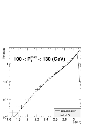
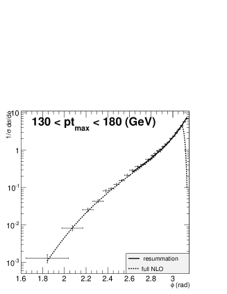
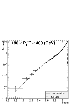
Figure 8: The comparisons between the theory calculations and the experimental data from the D0 collaboration at the Tevatron.

In Fig. 8, we plot the comparisons between our resummation result and the experimental data from D0 collaboration at Tevatron. For completeness, we also show the prediction of a fixed order calculation at the NLO Nagy:2001fj , which includes both one-loop $2\to 3$ and tree level $2\to 4$ contributions. To compare with the normalized differential cross section, we have normalized the result of our resummation calculation in $\phi_{\rm dijet}$ distribution by the LO dijet cross section, with both jets in the specified $p_{T}$ and $y$ bins of the data point. Namely, the normalization factor $\sigma_{\rm dijet}$ is taken to be the NLO dijet cross section in the NLO prediction, and the LO dijet cross section in the resummation prediction. This is because in our resummation calculation, cf. Eq. (417), the hard factor ${\bf H}$ is only kept at the LO in this calculation. From these plots, we can clearly see that the resummation results agree well with the experimental data around the back-to-back correlation region of $\phi\sim\pi$. For smaller value of $\phi$ (away from the back-to-back configuration), the resummation calculations match to the fixed order results at NLO Nagy:2001fj , which has also been separately shown in Fig. 8. We note that a full NLO calculation cannot describe experimental data for $\phi\sim\pi$ Abazov:2004hm , where the fixed order calculation becomes divergent. Our resummation calculation, after being matched with the NLO result clearly improves the theory prediction and can describe the experimental data in a wider kinematic region. This demonstrates the importance of all order resummation in perturbative calculations for these type of hard QCD processes.

VII.3 Dijet Correlations at the LHC

Dijet production processes are among the first few measurements of $pp$ collisions at the LHC. Both CMS and ATLAS have reported the experimental results on the azimuthal angular correlations of dijet productions, as done by the D0 Collaboration at the Tevatron.

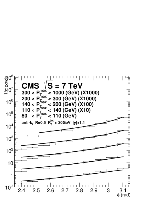
Figure 9: The comparisons between the resummation results and the experimental data from the CMS collaboration at the LHC. The kinematics of each bins are specified according to the experiment Khachatryan:2011zj .

In Fig. 9, we compare our resummation results with the experimental data from the CMS collaboration at the LHC. Similar to the D0 measurements, the dijet measurements are presented in several kinematic bins, with the leading jet transverse momentum labelled by $P_{T}^{max}$ in the figure. The second jet transverse momentum is chosen to be larger than $30$ GeV. Both jets are in the mid-rapidity region, $|y_{jet}|<1.1$. Anti-$k_{t}$ jet algorithm with jet size $R=0.5$ was used in the data analysis. We have also applied this algorithm in our calculations. In this figure, we limit the comparisons in the back-to-back correlation region, where we find perfect agreements between the resummation calculations and the experimental data over all transverse momentum bins. Similar to that in Fig. 8, away from the back-to-back region, the resummation calculations will match to the fixed order results.

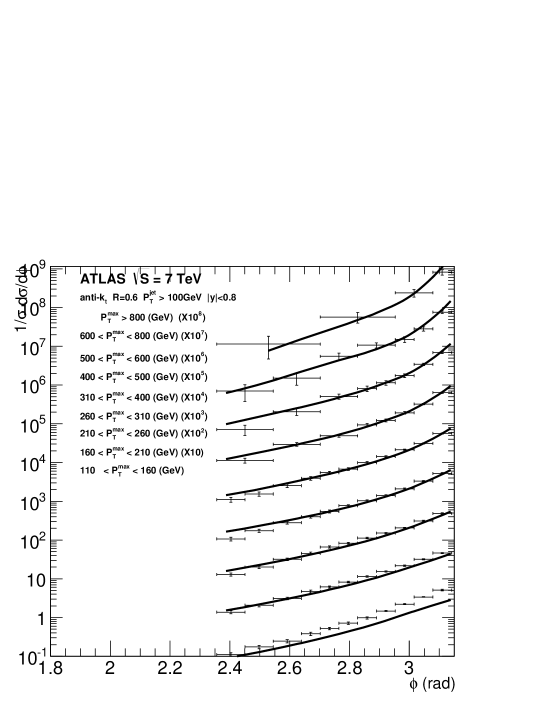
Figure 10: The comparisons between the theory calculations and the experimental data from the ATLAS Collaboration at the 7 TeV LHC.

In Fig. 10, we compare to the measurements form the ATLAS collaboration daCosta:2011ni . In this experiment, the same anti-$k_{t}$ algorithm has been used, however, with jet size $R=0.6$. The two jets are selected from the mid-rapidity region ($|y_{jet}|<0.8$) with minimum transverse momentum of 100 GeV. The data sets are chosen according to different leading jet transverse momentum region as indicated in the figure. From this figure, we can see that the agreements between the resummation results and the experimental data are very well around the back-to-back correlation regions, except in the lowest $P_{T}^{max}$ bin. The apparent poor agreement between the resummation prediction and the ATLAS data in the lowest $P_{T}^{max}$ bin (between 110 GeV and 160 GeV) is caused by the stronger kinematic cut made on the second jet $P_{T}$, which is required to be above 100 GeV at ATLAS and 30 GeV at CMS. With a much tighter cut on this second jet $P_{T}$, the phase space for multiple soft gluon emission is limited so that our resummation calculation (which allows all possible soft gluon radiation) becomes less reliable in this case. We note that in the lowest $P_{T}^{max}$ bin, the cross section is dominated by $P_{T}^{max}$ around 110 GeV which is close to the 100 GeV cut on the second jet made by the ATLAS.

VIII Summary and Discussions

In summary, in this paper, we have investigated all order soft gluon resummation in dijet production processes in hadronic collisions. The procedure and methodology follow the original CSS resummation for massive neutral particle production. Because the final state jets carry color, the resummation formulas have to be modified to include the effect of soft gluon radiation associated with the final state jets. In the derivation, we calculated the complete one-loop contributions from soft and collinear gluon radiations in all partonic channels in dijet productions. The soft divergences are shown to be cancelled out completely between real and virtual graphs, which provides an important check to our one-loop calculations. In order to derive an analytic expression with the jet cone size dependence to demonstrate the cancellations in the final results and to derive the resummation formula, we apply the narrow jet approximation in our calculations. We have also implement the (anti-$k_{t}$) jet algorithm to separate out the out-of-jet cone radiation from the gluon radiation inside the cone jet. Hence, the final results of our calculation depend on the jet algorithm and the jet size, which can then be directly compared to experimental data. As an important cross check, we have compared our derivation of soft and collinear gluon radiation contribution to the fixed order calculations at this order, and the numeric comparisons show that they agree very well in the kinematics of back-to-back correlation regions. In this region, because the predictions of fixed order calculations are divergent, we have to take into account all order resummation effects.

We have compared our resummation results to the experimental data from the measurements at the Tevatron and LHC. All these comparisons demonstrate that the resummation results are crucial to improve the theory descriptions of the experimental data around the azimuthal back-to-back kinematic region. The combination of the NLO perfurbative calculations (including both one-loop $2\to 3$ and tree level $2\to 4$ contributions) and our resummation results provide the most adequate theory descriptions to these experimental data.

Our calculations are the first systematic derivations of the TMD resummation for dijet production in hadronic collisions at the NLL order. The results have been cross checked through various perspectives, and they are consistent within the theoretical framework our calculations are built on. These cross checks are nontrivial supports for the factorization arguments used in our derivations. A number of extensions can be performed along this direction. For example, we shall be able to calculate the soft gluon resummation effects in the vector boson (or Higgs boson) plus a high $P_{T}$ jet production at the colliders where the total transverse momentum of the boson and the jet is much smaller than the invariant mass of the final state particles Sun:2014lna . These processes are important channels to study the Standard Model physics at the LHC.

Finally, we would like to comment on the applications of our results to the dijet production with large rapidity separation. This particular kinematics is very interesting to study the QCD resummation physics. It has long been realized that the so-called BFKL resummation Balitsky:1978ic will be important in this kinematics, which is referred as the Mueller-Navelet dijet production Mueller:1986ey . In particular, recently, the CMS collaboration at the LHC has measured the dijet azimuthal correlation with large rapidity separation between the jets, which has been interpreted as the BFKL resummation effects Ducloue:2013bva . However, in this calculation, only BFKL-type resummation has been taken into account. We would like to argue that there should be Sudakov resummation as well. Theoretically, how to resum large logarithms from both types of physics effects is an important question. We will not address it in this paper. Instead, we will discuss below the physics of our resummation formula when considered in this kinematics.

When the two jets are produced with large rapidity separation, we are in a special kinematic region, where the physics is dominated by $t$-channel diagrams. Therefore, we can apply the following kinematic approximations, $s\sim-u\gg-t$, which also implies that $P_{T}^{2}=tu/s\approx-t$. More importantly, all the partonic channels with $t$-channel gluon exchange will be the most important contributions. This is because they all have terms which are proportional to $s^{2}/t^{2}$. This includes the following channels: $qq^{\prime}\to qq^{\prime}$, $qg\to qg$, and $gg\to gg$. In addition, by applying the above approximation, we find out that the anomalous dimensions for the associated soft factors derived in the last section become diagonalized. The direct consequence is that we can simplify the final resummation formula, by absorbing the soft factor anomalous dimension of Eq. (417) into the overall Sudakov perturbative form factor of Eq. (418). This much simplified result, as compared to that presented in the last section, may indicate a consistent resummation formula for the Mueller-Navelet dijet production. The remaining task is to develop a consistent theoretical framework to include both physics effects induced by the BFKL and Sudakov resummation dynamics xiao .

- (1) V. M. Abazov et al. [D0 Collaboration], Phys. Rev. Lett. 94, 221801 (2005).
- (2) V. Khachatryan et al. [CMS Collaboration], Phys. Rev. Lett. 106, 122003 (2011).
- (3) G. Aad et al. [ATLAS Collaboration], Phys. Rev. Lett. 106, 172002 (2011).
- (4) Z. Nagy, Phys. Rev. Lett. 88, 122003 (2002); Phys. Rev. D 68, 094002 (2003).
- (5) P. Sun, C.-P. Yuan and F. Yuan, Phys. Rev. Lett. 113, no. 23, 232001 (2014) [arXiv:1405.1105 [hep-ph]].
- (6) J. C. Collins, D. E. Soper and G. F. Sterman, Nucl. Phys. B 250, 199 (1985). Kazuhiro Watanabe
- (7) A. Banfi, M. Dasgupta and Y. Delenda, Phys. Lett. B 665, 86 (2008).
- (8) A. H. Mueller, B. -W. Xiao and F. Yuan, Phys. Rev. D 88, 114010 (2013).
- (9) A. Banfi and M. Dasgupta, JHEP 0401, 027 (2004).
- (10) F. Hautmann and H. Jung, JHEP 0810, 113 (2008).
- (11) N. Kidonakis and G. F. Sterman, Nucl. Phys. B 505, 321 (1997); N. Kidonakis, G. Oderda and G. F. Sterman, Nucl. Phys. B 525, 299 (1998).
- (12) J. Botts and G. F. Sterman, Nucl. Phys. B 325, 62 (1989).
- (13) B. Jager, M. Stratmann and W. Vogelsang, Phys. Rev. D 70, 034010 (2004).
- (14) A. Mukherjee and W. Vogelsang, Phys. Rev. D 86, 094009 (2012).
- (15) R. K. Ellis and J. C. Sexton, Nucl. Phys. B 269, 445 (1986).
- (16) J. W. Qiu, W. Vogelsang and F. Yuan, Phys. Rev. D 76, 074029 (2007) [arXiv:0706.1196 [hep-ph]].
- (17) J. Collins and J. -W. Qiu, Phys. Rev. D 75, 114014 (2007).
- (18) T. C. Rogers and P. J. Mulders, Phys. Rev. D 81, 094006 (2010).
- (19) W. Vogelsang and F. Yuan, Phys. Rev. D 76, 094013 (2007).
- (20) S. Catani, D. de Florian and G. Rodrigo, JHEP 1207, 026 (2012).
- (21) A. Mitov and G. Sterman, Phys. Rev. D 86, 114038 (2012).
- (22) X. Ji, J. P. Ma and F. Yuan, Phys. Rev. D 71, 034005 (2005); JHEP 0507, 020 (2005).
- (23) J. Gao, M. Guzzi, J. Huston, H. -L. Lai, Z. Li, P. Nadolsky, J. Pumplin and D. Stump et al., Phys. Rev. D 89, 033009 (2014).
- (24) F. Landry, R. Brock, P. M. Nadolsky and C. P. Yuan, Phys. Rev. D 67, 073016 (2003); Phys. Rev. D 63, 013004 (2001); P. Sun, C. -P. Yuan and F. Yuan, Phys. Rev. D 88, 054008 (2013).
- (25) A. V. Konychev and P. M. Nadolsky, Phys. Lett. B 633, 710 (2006) [hep-ph/0506225].
- (26) P. Sun, J. Isaacson, C.-P. Yuan and F. Yuan, arXiv:1406.3073 [hep-ph].
- (27) P. Sun, C.-P. Yuan and F. Yuan, arXiv:1409.4121 [hep-ph].
- (28) I. I. Balitsky and L. N. Lipatov, Sov. J. Nucl. Phys. 28, 822 (1978) [Yad. Fiz. 28, 1597 (1978)]; E. A. Kuraev, L. N. Lipatov and V. S. Fadin, Sov. Phys. JETP 45, 199 (1977) [Zh. Eksp. Teor. Fiz. 72, 377 (1977)];
- (29) A. H. Mueller and H. Navelet, Nucl. Phys. B 282, 727 (1987).
- (30) B. Duclou, L. Szymanowski and S. Wallon, Phys. Rev. Lett. 112, 082003 (2014).
- (31) B.W. Xiao, et al., to be published.