CO2 Forest: Improved Random Forest by Continuous Optimization of Oblique Splits

Abstract

We propose a novel algorithm for optimizing multivariate linear threshold functions as split functions of decision trees to create improved Random Forest classifiers. Standard tree induction methods resort to sampling and exhaustive search to find good univariate split functions. In contrast, our method computes a linear combination of the features at each node, and optimizes the parameters of the linear combination (oblique) split functions by adopting a variant of latent variable SVM formulation. We develop a convex-concave upper bound on the classification loss for a one-level decision tree, and optimize the bound by stochastic gradient descent at each internal node of the tree. Forests of up to 1000 Continuously Optimized Oblique (CO2) decision trees are created, which significantly outperform Random Forest with univariate splits and previous techniques for constructing oblique trees. Experimental results are reported on multi-class classification benchmarks and on Labeled Faces in the Wild (LFW) dataset.

1 Introduction

Decision trees [6, 24] and random forests [13, 5] have a long, successful history in machine learning, in part due to their computational efficiency and their applicability to large-scale classification and regression tasks (e.g., see [11, 7]). A case in point is the Microsoft Kinect, where multiple decision trees are learned on millions of training exemplars to enable real time human pose estimation from depth images [27]. The standard algorithm for decision tree induction grows a tree one node at a time, greedily and recursively. The building block of this procedure is an optimization at each internal node of the tree, which divides the training data at that node into two subsets according to a splitting criterion, such as Gini impurity index in CART [6], or information gain in C4.5 [25]. This corresponds to optimizing a binary decision stump, or a one-level decision tree, at each internal node. Most tree-based methods exploit univariate (axis-aligned) split functions, which compare one feature dimension to a threshold. Optimizing univariate decision stumps is straightforward because one can exhaustively enumerate all plausible thresholds for each feature, and thereby select the best parameters according to the split criterion. Conversely, univariate split functions have limited discriminative power.

We investigate the use of a more general and powerful family of split functions, namely, linear-combination (a.k.a., oblique) splits. Such split functions comprise a multivariate linear projection of the features followed by binary quantization. Clearly, exhaustive search with linear hyperplanes is not feasible, and based on our preliminary experiments, random sampling yields poor results. Further, typical splitting criteria for a one-level decision tree (decision stump) are discontinuous, since small changes in split parameters may change the assignment of data to branches of the tree. As a consequence, split parameters are not readily amenable to numerical optimization, so oblique split functions have not been used widely with tree-based methods.

This paper advocates a new building block for learning decision trees, i.e., an algorithm for continuous optimization of oblique decision stumps. To this end, we introduce a continuous upper bound on the empirical loss associated with a decision stump. This upper bound resembles a ramp loss, and accommodates any convex loss that is useful for multi-class classification, regression, or structured prediction [22]. As explained below, the bound is the difference of two convex terms, the optimization of which is effectively accomplished using the Convex-Concave Procedure of [33]. The proposed bound resembles the bound used for learning binary hash functions [20].

Some previous work has also considered improving the classification accuracy of decision trees by using oblique split functions. For example, Murthy et al. [19] proposed a method called OC1, which yields some performance gains over CART and C4.5. Nevertheless, individual decision trees are rarely sufficiently powerful for many classification and regression tasks. Indeed, the power of tree-based methods often arises from diversity among the trees within a forest. Not surprisingly, a key question with optimized decision trees concerns the loss of diversity that occurs with optimization, and hence a reduction in the effectiveness of forests of such trees. The random forest of Breiman seems to achieve a good balance between optimization and randomness.

Our experimental results suggest that one can effectively optimize oblique split functions, and the loss of diversity associated with such optimized decision trees can be mitigated. In particular, it is found that when the decision stump optimization is initialized with random forest’s split functions, one can indeed construct a forest of non-correlated decision trees. We effectively take advantage of the underlying non-convex optimization problem, for which a diverse set of initial states for the optimizer yields a set of different split functions. Like random forests, the resulting algorithm achieves very good performance gains as the number of trees in the ensemble increases.

We assess the effectiveness of our tree construction algorithm by generating up to $1000$ decision trees on nine classification benchmarks. Our algorithm, called CO2 forest, outperforms random forest on all of the datasets. It is also shown to outperform a baseline of OC1 trees. As a large-scale experiment, we consider the task of segmenting faces from the Labeled Faces in the Wild (LFW) dataset [14]. Again, our results confirm that CO2 forest outperforms other baselines.

2 Related Work

Breiman et al. [6] proposed a version of CART that employs linear combination splits, known as CART-linear-combination (CART-LC). Murthy et al. [12, 19] proposed OC1, a refinement of CART-LC that uses random restarts and random perturbations to escape local minima. The main idea behind both algorithms is to use coordinate descent to optimize the parameters of the oblique splits one dimension at a time. Keeping all of the weights corresponding to an oblique decision stump fixed except one, for each datum they compute the critical value of the missing weight at which the datum switches its assignment to the branches. Then, one can sort these critical values to find the optimal value of each weight (with other weights fixed). By performing multiple passes over the dimensions and the data, oblique splits with small empirical loss can be found.

By contrast, our algorithm updates all the weights simultaneously using gradient descent. While the aforementioned algorithms focus mainly on optimizing the splitting criterion to minimize tree size, there is little promise of improved generalization. Here, by adopting a formulation based on the latent variable SVM [32], our algorithm provides a natural means of regularizing the oblique split stumps, thereby improving the generalization power of the trees.

The hierarchical mixture of experts (HME) [16] uses soft splits rather than hard binary decisions to capture situations where the transition from low to high response is gradual. The empirical loss associated with HME is a smooth function of the unknown parameters and hence numerical optimization is feasible. The main drawback of HME concerns inference. That is, multiple paths along the tree should be explored during inference, which reduces the efficiency of the classifier.

Our work builds upon random forest [5]. Random forest combines bootstrap aggregating (bagging) [4] and the random selection of features [13] to construct an ensemble of non-correlated decision trees. The method is used widely for classification and regression tasks, and research still investigates its theoretical characteristics [8]. Building on random forest, we also grow each tree using a bootstrapped version of the training dataset. The main difference is the way the split functions are selected. Training random forest is generally faster than using our optimized oblique trees, and because random forest uses univariate splits, classification with the same number of trees is often faster. Nevertheless, we often achieve similar accuracy with many fewer trees, and depending on the application, the gain in classification performance is clearly worth the computational overhead.

There also exist boosting based techniques for creating ensembles of decision trees [10, 34]. A key benefit of random forest over boosting is that it allows for faster training as the decision trees can be trained in parallel. In our experiments we usually train $30$ trees in parallel on a multicore machine. Nevertheless, it is interesting to combine boosting techniques with our oblique trees, and we leave this to future work.

Menze et al. [18] also consider a variant of oblique random forest. At each internal node they find an optimal split function using either ridge regression or linear discriminant analysis. Like other previous work [30, 3], the technique of [18] is only conveniently applicable to binary classification tasks. A big challenge in a multi-class setting is solving the combinatorial assignment of labels to the two leaves. In contrast to [18], our technique is more general, and allows for optimization of multi-class classification and regression loss functions.

Rota Buló & Kontschieder [26] recently proposed the use of multi-layer neural nets as split functions at internal nodes. While extremely powerful, the resulting decision trees lose their computational simplicity during training and testing. Further, it may be difficult to produce the required diversity among trees in a forest. This paper explores the middle ground, with a simple, yet effective class of linear multi-variate split functions. That said, note that the formulation of the upper bound used to optimize empirical loss in this paper can be extended to optimize other non-linear split functions, including neural nets (e.g.,[21]).

3 Preliminaries

For ease of exposition, this paper is focused on binary classification trees, with $m$ internal (split) nodes, and $m+1$ leaf (terminal) nodes. An input, ${\bm{\mathbf{x}}}\in\mathbb{R}^{p}$, is directed from the root of the tree down through internal nodes to a leaf node, which specifies a distribution over $k$ class labels.

Each internal node, indexed by $i\in\{1,\ldots,m\}$, performs a binary test by evaluating a node-specific split function $t_{i}({\bm{\mathbf{x}}}):\mathbb{R}^{p}\to\{-1,+1\}$. If $t_{i}({\bm{\mathbf{x}}})$ evaluates to $-1$, then ${\bm{\mathbf{x}}}$ is directed to the left child of node $i$. Otherwise, ${\bm{\mathbf{x}}}$ is directed to the right child. And so on down the tree. Each split function $t_{i}(\cdot)$, parametrized by a weight vector ${\bm{\mathbf{w}}}_{i}$, is assumed to be a linear threshold function of the form $t_{i}({\bm{\mathbf{x}}})=\operatorname{sgn}({{\bm{\mathbf{w}}}_{i}}^{\mathsf{T}}{\bm{\mathbf{x}}})$. We incorporate an offset parameter to obtain split functions of the form $\operatorname{sgn}({{\bm{\mathbf{w}}}_{i}}^{\mathsf{T}}{\bm{\mathbf{x}}}-b_{i})$ by using homogeneous coordinates (i.e., by appending a constant “$-1$” to the end of the input feature vector).

Each leaf node, indexed by $j\in\{0,\ldots,m\}$, specifies a conditional probability distribution over class labels, $l\in\{1,\ldots,k\}$, denoted $p({y}=l\mid j)$. These distributions are parameterized in terms of a vector of unnormalized predictive log-probabilities, denoted ${\bm{\mathbf{\theta}}}_{j}\in\mathbb{R}^{k}$, and a conventional softmax function; i.e.,

$$p({y}=l\mid j)~{}=~{}\frac{\exp\left\{{\bm{\mathbf{\theta}}}_{j[l]}\right\}}{\sum_{\alpha=1}^{k}\exp\left\{{\bm{\mathbf{\theta}}}_{j[\alpha]}\right\}}~{},$$ (1)

where ${\bm{\mathbf{v}}}_{[\alpha]}$ denotes the $\alpha^{\mathrm{th}}$ element of vector ${\bm{\mathbf{v}}}$.

The parameters of the tree comprise the $m$ internal weight vectors, each of dimension $p+1$, and the $m+1$ vectors of unnormalized log-probabilities, one for each leaf node, i.e., $\{{\bm{\mathbf{w}}}_{i}\}_{i=1}^{m}$ and $\{{\bm{\mathbf{\theta}}}_{j}\}_{j=0}^{m}$. Given a dataset of input-output pairs, $\mathcal{D}\equiv\{{\bm{\mathbf{x}}}_{z},{y}_{z}\}_{z=1}^{n}$, where ${y}_{z}\in\{1,\ldots,k\}$ is the ground truth class label associated with input ${\bm{\mathbf{x}}}_{z}\in\mathbb{R}^{p}$, we wish to find a joint configuration of oblique splits $\{{\bm{\mathbf{w}}}_{i}\}_{i=1}^{m}$ and leaf parameters $\{{\bm{\mathbf{\theta}}}_{j}\}_{j=0}^{m}$ that minimize some measure of misclassification loss on the training set. Joint optimization of the split functions and leaf parameters according to a global objective is, however, known to be extremely challenging [15] due to the discrete and sequential nature of the decisions within the tree.

To cope with the discontinuous objective caused by discrete split functions, we propose a smooth upper bound on the empirical loss, with which one can effectively learn a diverse collection of trees with oblique split functions. We apply this approach to the optimization of split functions of internal nodes within the context of a top-down greedy induction procedure, one in which each internal node is treated as an independent one-level decision stump. The split functions of the tree are optimized one node at a time, in a greedy fashion as one traverses the tree, breadth first, from the root downward. The procedure terminates when a desired tree depth is reached, or when some other stopping criterion is met. While we focus here on the optimization of a single stump, the formulation can be generalized to optimize entire trees.

4 Continuous Optimization of Oblique (CO2) Decision Stumps

A binary decision stump is parameterized by a weight vector ${\bm{\mathbf{w}}}$, and two vectors of unnormalized log-probabilities for the two leaf nodes, ${\bm{\mathbf{\theta}}}_{0}$ and ${\bm{\mathbf{\theta}}}_{1}$. The stump’s loss function comprises two terms, one for each leaf, denoted $\ell({\bm{\mathbf{\theta}}}_{0},{y})$ and $\ell({\bm{\mathbf{\theta}}}_{1},{y})$, where $\ell:\mathbb{R}^{k}\times\{1,\ldots,k\}\to\mathbb{R}^{+}$. They measure the discrepancy between the label $y$ and the distributions parameterized by ${\bm{\mathbf{\theta}}}_{0}$ and ${\bm{\mathbf{\theta}}}_{1}$. The binary test at the root of the stump acts as a gating function to select a leaf, and hence its associated loss. The empirical loss for the stump, i.e., the sum of the loss over the training set $\cal{D}$, is defined as

$$\mathcal{L} \left({\bm{\mathbf{w}}},{\bm{\mathbf{\theta}}}_{0,1};\mathcal{D}\right)~{}=$$ (2)

$$\sum_{({\bm{\mathbf{x}}},{y})\in\mathcal{D}}\mathbbm{1}({{\bm{\mathbf{w}}}}^{\mathsf{T}}{\bm{\mathbf{x}}}<0)\,\ell({\bm{\mathbf{\theta}}}_{0},{y})+\mathbbm{1}({{\bm{\mathbf{w}}}}^{\mathsf{T}}{\bm{\mathbf{x}}}\geq 0)\,\ell({\bm{\mathbf{\theta}}}_{1},{y})~{},$$

where $\mathbbm{1}(\cdot)$ is the usual indicator function. Given the softmax model of Eq. (1), the log loss takes the form

$$\ell_{\log}({\bm{\mathbf{\theta}}},{y})\,=\,-{\bm{\mathbf{\theta}}}_{[{y}]}+\log\left\{\sum\nolimits_{\alpha=1}^{k}\exp\left\{{\bm{\mathbf{\theta}}}_{[\alpha]}\right\}\right\}~{}.$$ (3)

Regarding this formulation, we note that the parameters which minimize Eq. (2) with the log loss, $\ell_{\log}$, are those that maximize information gain. One can prove this with straightforward algebraic manipulation of Eq. (2), recognizing that the ${\bm{\mathbf{\theta}}}_{0}$ and ${\bm{\mathbf{\theta}}}_{1}$ that minimize Eq. (2), given any ${\bm{\mathbf{w}}}$, are the empirical class log-probabilities at the leaves.

We also note that the framework outlined below accommodates other loss functions that are convex in ${\bm{\mathbf{\theta}}}$. For instance, for regression tasks where ${\bm{\mathbf{y}}}\in\mathbb{R}^{k}$, one can use squared loss,

$$\ell_{\text{sqr}}({\bm{\mathbf{\theta}}},{\bm{\mathbf{y}}})\,=\,\lVert{\bm{\mathbf{\theta}}}-{\bm{\mathbf{y}}}\rVert_{2}^{2}~{}~{}.$$ (4)

As mentioned already above, it is also important to note that empirical loss, $\mathcal{L}({\bm{\mathbf{w}}},{\bm{\mathbf{\theta}}}_{0,1};\mathcal{D})$, is a discontinuous function of ${\bm{\mathbf{w}}}$. As a consequence, optimization of $\mathcal{L}$ with respect to ${\bm{\mathbf{w}}}$ is very challenging. Our approach, outlined in detail below, is to instead optimize a continuous upper bound on empirical loss. This bound is closely related to formulations of binary SVM and logistic regression classification. In the case of binary classification, the assignment of class labels to each side of the hyperplane, i.e., the parameters ${\bm{\mathbf{\theta}}}_{0}$ and ${\bm{\mathbf{\theta}}}_{1}$, are pre-specified. In contrast, a decision stump with a large numbers of labels entails joint optimization of both the assignment of the labels to the leaves and the hyperplane parameters.

4.1 Upper Bound on Empirical Loss

The upper bound on loss that we employ, given an input-output pair $({\bm{\mathbf{x}}},{y})$, has the following form:

$$\mathbbm{1}({{\bm{\mathbf{w}}}}^{\mathsf{T}}{\bm{\mathbf{x}}}<0)\,\ell({\bm{\mathbf{\theta}}}_{0},{y})+\mathbbm{1}({{\bm{\mathbf{w}}}}^{\mathsf{T}}{\bm{\mathbf{x}}}\geq 0)\,\ell({\bm{\mathbf{\theta}}}_{1},{y})\leq$$ (5)

$$\max\big{(}\!-{{\bm{\mathbf{w}}}}^{\mathsf{T}}{\bm{\mathbf{x}}}\!+\!\ell({\bm{\mathbf{\theta}}}_{0},{y})~{},~{}{{\bm{\mathbf{w}}}}^{\mathsf{T}}{\bm{\mathbf{x}}}+\ell({\bm{\mathbf{\theta}}}_{1},{y})\big{)}-\lvert{{\bm{\mathbf{w}}}}^{\mathsf{T}}{\bm{\mathbf{x}}}\rvert~{},$$

where $\lvert{{\bm{\mathbf{w}}}}^{\mathsf{T}}{\bm{\mathbf{x}}}\rvert$ denotes the absolute value of ${{\bm{\mathbf{w}}}}^{\mathsf{T}}{\bm{\mathbf{x}}}$. To verify the bound, first suppose that ${{\bm{\mathbf{w}}}}^{\mathsf{T}}{\bm{\mathbf{x}}}<0$. In this case, it is straightforward to show that the inequality reduces to

$$\ell({\bm{\mathbf{\theta}}}_{0},{y})\,\leq\,\max\big{(}\ell({\bm{\mathbf{\theta}}}_{0},{y})~{},~{}2\,{{\bm{\mathbf{w}}}}^{\mathsf{T}}{\bm{\mathbf{x}}}+\ell({\bm{\mathbf{\theta}}}_{1},{y})\big{)}~{},$$ (6)

which holds trivially. Conversely, when ${{\bm{\mathbf{w}}}}^{\mathsf{T}}{\bm{\mathbf{x}}}\geq 0$ the inequality reduces to

$$\ell({\bm{\mathbf{\theta}}}_{1},{y})\,\leq\,\max\big{(}\!-2\,{{\bm{\mathbf{w}}}}^{\mathsf{T}}{\bm{\mathbf{x}}}+\ell({\bm{\mathbf{\theta}}}_{0},{y})~{},~{}\ell({\bm{\mathbf{\theta}}}_{1},{y})\big{)}~{},$$ (7)

which is straightforward to validate. Hence the inequality in Eq. (5) holds.

Interestinly, while empirical loss in Eq. (2) is invariant to $\lVert{\bm{\mathbf{w}}}\rVert$, the bound in Eq. (6) is not. That is, for any real scalar $a>0$, $\operatorname{sgn}(a{{\bm{\mathbf{w}}}}^{\mathsf{T}}{\bm{\mathbf{x}}})$ does not change with $a$, and hence $\mathcal{L}({\bm{\mathbf{w}}},{\bm{\mathbf{\theta}}}_{0,1})=\mathcal{L}(a{\bm{\mathbf{w}}},{\bm{\mathbf{\theta}}}_{0,1})$. Thus, while the loss on the LHS of Eq. (5) is scale-invariant, the upper bound on the RHS of Eq. (5) does depend on $\lVert{\bm{\mathbf{w}}}\rVert$. Indeed, like the soft-margin binary SVM formulation, and margin rescaling formulations of structural SVM [31], the norm of ${\bm{\mathbf{w}}}$ affects the interplay between the upper bound and empirical loss. In particular, as the scale of ${\bm{\mathbf{w}}}$ increases, the upper bound becomes tighter and its optimization becomes more similar to a direct loss minimization.

More precisely, the upper bound becomes tighter as $\lVert{\bm{\mathbf{w}}}\rVert$ increases. This is evident from the following inequality, which holds for any real scalar $a>1$:

$$\!\!\!\!\!\max\big{(}\!\!-\!{{\bm{\mathbf{w}}}}^{\mathsf{T}}{\bm{\mathbf{x}}}\!+\!\ell({\bm{\mathbf{\theta}}}_{0},{y}),\,{{\bm{\mathbf{w}}}}^{\mathsf{T}}{\bm{\mathbf{x}}}\!+\!\ell({\bm{\mathbf{\theta}}}_{1},{y})\big{)}-\lvert{{\bm{\mathbf{w}}}}^{\mathsf{T}}{\bm{\mathbf{x}}}\rvert~{}\geq$$ (8)

$$~{}\max\big{(}\!\!-\!a{{\bm{\mathbf{w}}}}^{\mathsf{T}}{\bm{\mathbf{x}}}\!+\!\ell({\bm{\mathbf{\theta}}}_{0},{y}),\,a{{\bm{\mathbf{w}}}}^{\mathsf{T}}{\bm{\mathbf{x}}}\!+\!\ell({\bm{\mathbf{\theta}}}_{1},{y})\big{)}-a\lvert{{\bm{\mathbf{w}}}}^{\mathsf{T}}{\bm{\mathbf{x}}}\rvert~{}.$$

To verify the bound, as above, consider the sign of ${{\bm{\mathbf{w}}}}^{\mathsf{T}}{\bm{\mathbf{x}}}$. When ${{\bm{\mathbf{w}}}}^{\mathsf{T}}{\bm{\mathbf{x}}}<0$, inequality in Eq. (8) is equivalent to

$$\max\big{(}\ell({\bm{\mathbf{\theta}}}_{0},{y})~{},{} 2\,{{\bm{\mathbf{w}}}}^{\mathsf{T}}{\bm{\mathbf{x}}}+\ell({\bm{\mathbf{\theta}}}_{1},{y})\big{)}~{}\geq$$

$$\!\!\!\!\!\!\!\!\max\big{(}\ell({\bm{\mathbf{\theta}}}_{0},{y})~{},~{}2\,a{{\bm{\mathbf{w}}}}^{\mathsf{T}}{\bm{\mathbf{x}}}+\ell({\bm{\mathbf{\theta}}}_{1},{y})\big{)}~{}.$$

Conversely, when ${{\bm{\mathbf{w}}}}^{\mathsf{T}}{\bm{\mathbf{x}}}\geq 0$, Eq. (8) is equivalent to

$$\max\big{(}\!-2\,{{\bm{\mathbf{w}}}}^{\mathsf{T}}{\bm{\mathbf{x}}}+ \ell({\bm{\mathbf{\theta}}}_{0},{y})~{},~{}\ell({\bm{\mathbf{\theta}}}_{1},{y})\big{)}~{}\geq$$

$$\!\!\!\!\!\!\!\!\max\big{(}\!-2\,a{{\bm{\mathbf{w}}}}^{\mathsf{T}}{\bm{\mathbf{x}}}+\ell({\bm{\mathbf{\theta}}}_{0},{y})~{},~{}\ell({\bm{\mathbf{\theta}}}_{1},{y})\big{)}~{}.$$

Thus, as $\lVert{\bm{\mathbf{w}}}\rVert$ increases the bound becomes tighter. In the limit, as $\lVert{\bm{\mathbf{w}}}\rVert$ becomes large, the loss terms $\ell({\bm{\mathbf{\theta}}}_{0},{y})$ and $\ell({\bm{\mathbf{\theta}}}_{1},{y})$ become negligible compared to the terms $-{{\bm{\mathbf{w}}}}^{\mathsf{T}}{\bm{\mathbf{x}}}$ and ${{\bm{\mathbf{w}}}}^{\mathsf{T}}{\bm{\mathbf{x}}}$, in which case the RHS of Eq. (5) equals its LHS, except when ${{\bm{\mathbf{w}}}}^{\mathsf{T}}{\bm{\mathbf{x}}}\approx 0$. Hence, for large $\lVert{\bm{\mathbf{w}}}\rVert$, not only the bound gets tight, but also it becomes less smooth and more difficult to optimize in our nonconvex setting.

From the derivation above, and through experiments below, we observe that when $\lVert{\bm{\mathbf{w}}}\rVert$ is constrained, optimization converges to better solutions that exhibit better generalization. Summing over the bounds for the training pairs, and restricting $\lVert{\bm{\mathbf{w}}}\rVert$, we obtain the surrogate objective we aim to optimize to find the decision stump parameters:

$$\begin{aligned} &\mathrm{minimize}~{}~{}\mathcal{L}^{\prime}\left({\bm{\mathbf{w}}},{\bm{\mathbf{\theta}}}_{0,1};\mathcal{D},\nu\right)\\ &~{}~{}~{}~{}\text{such that}~{}~{}~{}\lVert{\bm{\mathbf{w}}}\rVert^{2}\leq\nu~{},\end{aligned}$$ (9)

where $\nu\in\mathbb{R}^{+}$ is a regularization parameter, and $\mathcal{L}^{\prime}$ is the surrogate objective, i.e., the upper bound,

$$\mathcal{L}^{\prime} \left({\bm{\mathbf{w}}},{\bm{\mathbf{\theta}}}_{0,1};\mathcal{D},\nu\right)~{}\equiv$$ (10)

$$\sum_{({\bm{\mathbf{x}}},{y})\in\mathcal{D}}\!\!\max\big{(}\!\!-\!{{\bm{\mathbf{w}}}}^{\mathsf{T}}{\bm{\mathbf{x}}}\!+\!\ell({\bm{\mathbf{\theta}}}_{0},{y}),{{\bm{\mathbf{w}}}}^{\mathsf{T}}{\bm{\mathbf{x}}}\!+\!\ell({\bm{\mathbf{\theta}}}_{1},{y})\big{)}-\lvert{{\bm{\mathbf{w}}}}^{\mathsf{T}}{\bm{\mathbf{x}}}\rvert~{}.$$

For all values of $\nu$, we have that $\mathcal{L}^{\prime}({\bm{\mathbf{w}}},{\bm{\mathbf{\theta}}}_{0,1};\mathcal{D},\nu)\geq\mathcal{L}({\bm{\mathbf{w}}},{\bm{\mathbf{\theta}}}_{0,1};\mathcal{D})$. We find a suitable $\nu$ via cross-validation. Instead of using the typical Lagrange form for regularization, we employed hard constraints with similar behavior.

4.2 Convex-Concave Optimization

Minimizing the surrogate objective in Eq. (10) entails nonconvex optimization. While still challenging, it is important that $\mathcal{L}^{\prime}\left({\bm{\mathbf{w}}},{\bm{\mathbf{\theta}}}_{0,1};\mathcal{D},\nu\right)$ is better behaved than empirical loss. It is piecewise smooth and convex-concave in ${\bm{\mathbf{w}}}$, and the constraint on ${\bm{\mathbf{w}}}$ defines a convex set. As a consequence, gradient-based optimization is applicable, although the surrogate objective is non-differentiable at isolated points. The objective also depends on the leaf parameters, ${\bm{\mathbf{\theta}}}_{0}$ and ${\bm{\mathbf{\theta}}}_{1}$, but only through the loss terms $\ell$, which we constrained to be convex in ${\bm{\mathbf{\theta}}}$. Therefore, for a fixed ${\bm{\mathbf{w}}}$, it follows that $\mathcal{L}^{\prime}\left({\bm{\mathbf{w}}},{\bm{\mathbf{\theta}}}_{0,1};\,\mathcal{D},\nu\right)$ is convex in ${\bm{\mathbf{\theta}}}_{0}$ and ${\bm{\mathbf{\theta}}}_{1}$.

The convex-concave nature of the surrogate objective allows us to use difference of convex (DC) programming, or the Convex-Concave Procedure (CCCP) [33], a method for minimizing objective functions expressed as sum of a convex and a concave term. The CCCP has been employed by Felzenszwalb et al. [9] and Yu & Joachims [32] to optimize latent variable SVM models that employ a similar convex-concave surrogate objective.

The Convex-Concave Procedure is an iterative method. At each iteration the concave term ($-\lvert{{\bm{\mathbf{w}}}}^{\mathsf{T}}{\bm{\mathbf{x}}}\rvert$ in our case) is replaced with its tangent plane at the current parameter estimate, to formulate a convex subproblem. The parameters are updated with those that minimize the convex subproblem, and then the tangent plane is updated. Let ${{\bm{\mathbf{w}}}}^{(old)}$ denote the estimate for ${\bm{\mathbf{w}}}$ from the previous CCCP iteration. In the next iteration ${{\bm{\mathbf{w}}}}^{(old)}$, ${\bm{\mathbf{\theta}}}_{0}$, and ${\bm{\mathbf{\theta}}}_{1}$ are updated minimizing

$$\sum_{({\bm{\mathbf{x}}},{y})\in\mathcal{D}}\Bigl{(}\max\big{(}\!\!-\!{{\bm{\mathbf{w}}}}^{\mathsf{T}}{\bm{\mathbf{x}}} \!+\!\ell({\bm{\mathbf{\theta}}}_{0},{y}),{{\bm{\mathbf{w}}}}^{\mathsf{T}}{\bm{\mathbf{x}}}\!+\!\ell({\bm{\mathbf{\theta}}}_{1},{y})\big{)}$$ (11)

$$-\operatorname{sgn}({{{\bm{\mathbf{w}}}}^{(old)}}^{\mathsf{T}}{\bm{\mathbf{x}}})\,{{\bm{\mathbf{w}}}}^{\mathsf{T}}{\bm{\mathbf{x}}}\Bigr{)}~{},$$

such that $\lVert{\bm{\mathbf{w}}}\rVert^{2}\leq\nu$.

Note that ${{\bm{\mathbf{w}}}}^{(old)}$ is constant during optimization of this CCCP subproblem. In that case, the second term within the sum over training data in Eq. (11) just defines a hyperplane in the space of ${\bm{\mathbf{w}}}$. The other (first) term within the sum entails maximization of a function that is convex in ${\bm{\mathbf{w}}}$, ${\bm{\mathbf{\theta}}}_{0}$ and ${\bm{\mathbf{\theta}}}_{1}$, since the maximum of two convex functions is convex. As a consequence, the objective of Eq. (11) is convex.

We use stochastic subgradient descent to minimize Eq. (11). After each subgradient update, ${\bm{\mathbf{w}}}$ is projected back into the feasible region. For efficiency, we do not wait for complete convergence of the convex subproblem within CCCP. Instead, ${{\bm{\mathbf{w}}}}^{(old)}$ is updated after a fixed number of epochs (denoted $\tau$) over the training dataset. The pseudocode for the optimization procedure is outlined in Alg 1.

Algorithm 1 The convex-concave procedure for Continuous Optimization of Oblique (CO2) decision stumps that minimizes Eq. (9) to estimate (${\bm{\mathbf{w}}}$, ${\bm{\mathbf{\theta}}}_{0}$, ${\bm{\mathbf{\theta}}}_{1}$) given a training dataset $\mathcal{D}$, and a hyper-parameter $\nu$ that constrains the norm of ${\bm{\mathbf{w}}}$

. 1:  Initialize ${\bm{\mathbf{w}}}$ by a random univariate split 2:  Estimate ${\bm{\mathbf{\theta}}}_{0}$, and ${\bm{\mathbf{\theta}}}_{1}$ based on ${\bm{\mathbf{w}}}$ and $\mathcal{D}$ 3:  while surrogate objective has not converged do 4:     ${{\bm{\mathbf{w}}}}^{(old)}\leftarrow{{\bm{\mathbf{w}}}}$ 5:     for $t=1$ to $\tau$ do 6:        sample a pair $({\bm{\mathbf{x}}},{y})$ at random from $\mathcal{D}$ 7:        $s\leftarrow\operatorname{sgn}({{\bm{\mathbf{w}}}}^{(old)}{\bm{\mathbf{x}}})$ 8:        if $-{{\bm{\mathbf{w}}}}^{\mathsf{T}}{\bm{\mathbf{x}}}+\ell({\bm{\mathbf{\theta}}}_{0},{y})\geq{{\bm{\mathbf{w}}}}^{\mathsf{T}}{\bm{\mathbf{x}}}+\ell({\bm{\mathbf{\theta}}}_{1},{y})$ then 9:           ${{\bm{\mathbf{w}}}}\leftarrow{{\bm{\mathbf{w}}}}+\eta(1+s){{\bm{\mathbf{x}}}}$ 10:           ${{\bm{\mathbf{\theta}}}_{0}}\leftarrow{{\bm{\mathbf{\theta}}}_{0}}-\eta\,\partial\ell({\bm{\mathbf{\theta}}}_{0},{y})/\partial{\bm{\mathbf{\theta}}}$ 11:        else 12:           ${{\bm{\mathbf{w}}}}\leftarrow{{\bm{\mathbf{w}}}}-\eta(1-s){{\bm{\mathbf{x}}}}$ 13:           ${{\bm{\mathbf{\theta}}}_{1}}\leftarrow{{\bm{\mathbf{\theta}}}_{1}}-\eta\,\partial\ell({\bm{\mathbf{\theta}}}_{1},{y})/\partial{\bm{\mathbf{\theta}}}$ 14:        end if 15:        if $\lVert{\bm{\mathbf{w}}}\rVert_{2}^{2}>\nu$ then 16:           ${{\bm{\mathbf{w}}}}\leftarrow\sqrt{\nu}\cdot{{\bm{\mathbf{w}}}}/\lVert{\bm{\mathbf{w}}}\rVert_{2}$ 17:        end if 18:     end for 19:  end while

In practice, we implement Alg 1 with several small modifications. Instead of estimating the gradients based on a single data point, we use mini-batches of $100$ elements, and average their gradients. We also use a momentum term of $0.9$ to converge more quickly. Finally, although a constant learning rate $\eta$ is used in Alg 1, we instead track the value of the surrogate objective, and when it oscillates for more than a number of iterations we reduce the learning rate.

5 Implementation and Experimental Details

In all tree construction methods considered here, we grow each decision tree as deep as possible, until we reach a pure leaf. We exploit the bagging ensemble learning algorithm [4] to create the forest such that each tree is built by using a new data set sampled uniformly with replacement from the original dataset. In Random Forest, for finding each univariate split function we only consider a candidate set of size $q$ of random feature dimensions, where $q$ is the only hyper-parameter in our random forest implementation. We set the parameter $q$ by growing a forest of $1000$ trees and testing them on a hold-out validation set of size $20\%$ of the training set. Let $p$ denote the dimensionality of the feature descriptors. We choose $q$ from the candidate set of $\{p^{0.5},p^{0.6},p^{0.7},p^{0.8},p^{0.9}\}$ to accelerate validation. Some previous work suggests the use of $q=\sqrt{p}$ as a heuristic [11], which is included in the candidate set.

We use an OC1 implementation provided by the authors [1]. We slightly modified the code to allow trees to grow to their fullest extent, removing hard-coded limits on tree depth and minimum examples for computing splits. We also modified the initialization of OC1 optimization to match our initialization for CO2, whereby an optimal axis-aligned split on a subsampling of $q$ possible features is used. Interestingly, we observed that both changes improve OC1’s performance when building ensembles of multiple trees, OC1 Forest. We use the default values provided by the authors for OC1 hyperparameters.

CO2 Forest has three hyper-parameters, namely, the regularization parameter $\nu$, the initial learning rate $\eta$, and $q$, the size of feature candidate set of which the best is selected to initialize the CO2 optimization. Ideally, one may consider using different regularizer parameters for different internal nodes of the tree, since the number of available training data decreases as one descends the tree. However, we use the same regularizer and learning rate for all of the nodes to keep hyper-parameter tuning simple. We set $q$ as selected by the random forest validation above. We perform a grid search over $\nu$ and $\eta$ to select the best hyper-parameters.

6 Experiments

Before presenting the classification results, we investigate the impact of the hyper-parameter $\nu$ on our oblique decision trees. Fig. 1 depicts training and validation error rates for the MNIST dataset for different values of $\nu\in\{0.1,1,10,100\}$ and different tree depths. One can see that as the tree depth increases, training error rate decreases monotonically. However, validation error rate saturates at a certain depth, e.g., a depth of $10$ for MNIST. Growing the trees deeper beyond this point, either has no impact, or slightly hurts the performance. From the plots it appears that $\nu=10$ exhibits the best training and validation error rates. The difference between different values of $\nu$ seems to be larger for validation error.

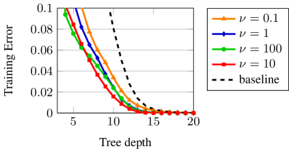
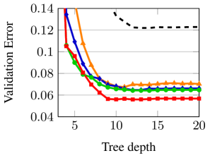
Figure 1: The impact of hyper-parameter $\nu$ on MNIST training and validation error rates for CO2 decision trees. The dashed baseline represents univariate decision trees with no pruning.

As shown above in Eq. (8), as $\nu$ increases the upper bound becomes tighter. Thus, one might suspect that larger $\nu$ implies a better optimum and better training error rates. However, increasing $\nu$ not only tightens the bound, but also makes the objective less smooth and harder to optimize. For MNIST, at $\nu=10$ there appears to be a reasonable balance between the tightness of the bound and the smoothness of the objective. The hyper-parameter $\nu$ also acts as a regularizer, contributing to the large gap in the validation error rates. For completeness, we also include baseline results with univariate decision trees. Clearly, the CO2 trees reach the same training error rates as the baseline but at a smaller depth. As seen from the validation error rates, the CO2 trees achieve better generalization too.

Classification results for tree ensembles are generally much better than a single tree. Here, we compare our Continuously Optimized Oblique (CO2) decision forest with random forest [5] and OC1 forest, forest built using OC1 [19]. Results for random forest are obtained with the implementation of the scikit-learn package [23]. Both of the baselines use information gain as the splitting criterion for learning decision stumps. We do not directly compare with other types of classifiers, as our research concerns tree-based techniques. Nevertheless, the reported results are often competitive with the state-of-the-art.

6.1 UCI multi-class benchmarks

					Test error (%) with different number of trees
Dataset Information					Random Forest			OC1 Forest			CO2 Forest
Name	#Train	#Test	#Class	Dim	10	30	1000	10	30	1000	10	30	1000
SatImage	$4,435$	$2,000$	$6$	$36$	10.1	9.4	8.9	10.1	9.9	9.5	9.6	9.1	8.9
USPS	$7,291$	$2,007$	$10$	$256$	9.0	7.2	6.4	7.1	7.1	6.8	5.8	5.9	5.5
Pendigits	$7,494$	$3,498$	$10$	$16$	3.9	3.3	3.5	3.2	2.2	2.3	1.8	1.7	1.7
Letter	$15,000$	$5,000$	$26$	$16$	6.6	4.7	3.7	7.6	5.0	3.8	3.2	2.3	1.8
Protein	$17,766$	$6,621$	$3$	$357$	39.9	35.5	30.9	39.1	34.6	30.8	33.8	31.2	30.3
Connect4∗	$55,000$	$12,557$	$3$	$126$	18.9	17.4	16.2	N/A			17.1	15.7	14.7
MNIST	$60,000$	$10,000$	$10$	$784$	4.5	3.5	2.8	N/A			2.5	2.0	1.9
SensIT	$78,823$	$19,705$	$3$	$100$	15.5	14.0	13.4	N/A			14.1	13.0	12.5
Covertype∗	$500,000$	$81,012$	$7$	$54$	3.2	2.8	2.6	N/A			3.1	2.7	2.6

TABLE I: Test error rates for forests with different number of trees on multi-class classification benchmarks. First few columns provide dataset information. Test error rates (%) for random forest, OC1 Forest, and CO2 Forest with $10$, $30$, and $1000$ trees are reported. For datasets marked with a star “^∗” (i.e., Connect4 & Covertype) we use our own training and test splits. As the number of training data points and feature dimensionality increase, OC1 becomes prohibitively slow, so this method is not applicable to the datasets with high-dimensional data or large training sets.

We conduct experiments on nine UCI multi-class benchmarks, namely, SatImage, USPS, Pendigits, Letter, Protein, Connect4, MNIST, SensIT, Covertype. Table I provides a summary of the datasets, including the number of training and test points, the number of class labels, and the feature dimensionality. We use the training and test splits set by previous work, except for Connect4 and Covertype. More details about the datasets, including references to the corresponding publications can be found at the LIBSVM dataset repository page [2].

Test error rates for random forest, OC1 Forest, and CO2 Forest with different numbers of trees ($10$, $30$, $1000$) are reported in Table I. OC1 results are not presented on some datasets, as the derivative-free coordinate descent method used does not scale to large or high-dimensional datasets, e.g., requiring more than $24$ hours to train a single tree on MNIST. CO2 Forest consistently outperforms random forest and OC1 Forest on all of the datasets. In some cases, i.e., Covertype, and SatImage, the improvement is small, but in four of the datasets CO2 Forest with only $10$ trees outperforms random forest with $1000$ trees.

For all methods, there is a large performance gain when the number of trees is increased from $10$ to $30$. The marginal gain from $30$ to $1000$ trees is less significant, but still notable. Finally, we also plot test error curves as a function of log number of trees in Fig. 2. CO2 Forest outperforms random forest and OC1 by a large margin and in most cases the marginal gain persists across different number of trees. For some datasets, OC1 Forest outperforms random forest, but it consistently underperforms CO2 Forest.

For pre-processing, the datasets are scaled so that either the feature dimensions are in the range of $[0,1]$, or they have a zero mean and a unit standard deviation. For CO2 Forest, we select $\nu$ from the set $\{0.1,1,4,10,43,100\}$, and $\eta$ from the set $\{.03,.01,.003\}$. A validation of $30$ decision trees is performed over $18$ entries of the grid of $(\nu,\eta)$.

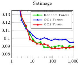
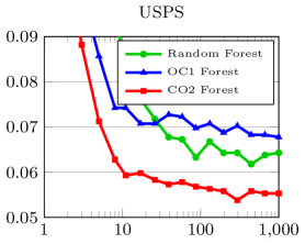
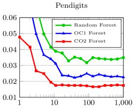
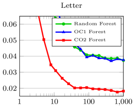
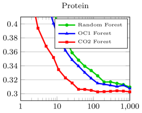
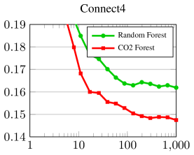
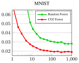
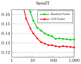
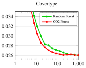
Figure 2: Test error curves for Random Forest and OC1 Forest vs. CO2 Forest as a function of (log) number of trees on the multi-class classification benchmarks. On the last four datasets, OC1 implementation is prohibitively slow, hence not applicable.

6.2 Labeled Faces in the Wild (LFW)

Input	Ground truth	Axis-aligned	Two-probe	CO2	Input	Ground truth	Axis-aligned	Two-probe	CO2

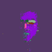
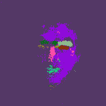
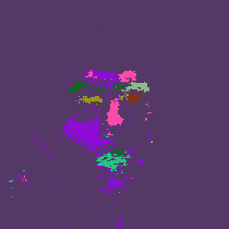
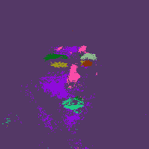
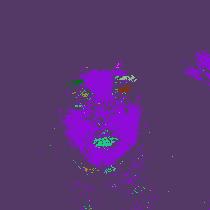
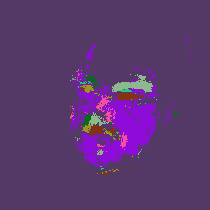
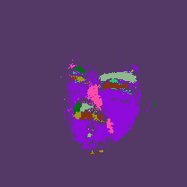
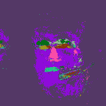
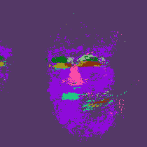
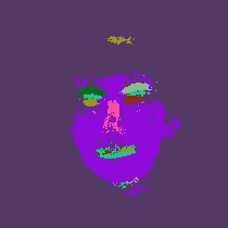
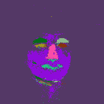
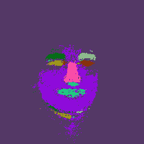
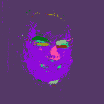
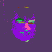
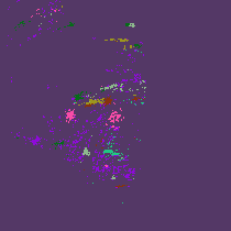
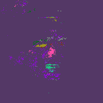
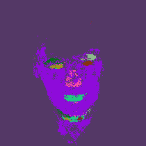
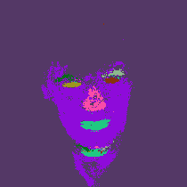
Figure 3: The above shows side-by-side comparisons of classification results on images from the test set. From left to right, these are the input image, the ground truth labels, the outputs of Random Forest, Two-probe Forest, and CO2 Forest. The first column depicts images chosen to show a spread of different segmentation qualities with the first three the median image by Jaccard score for each method, and the last two, examples with highest mean and variance in scores across methods. The second column shows five random examples.

As a large-scale experiment, we consider the task of segmenting face parts based on the Labeled Faces in the Wild (LFW) dataset [14]. We seek to label image pixels that belong to one of the following $7$ face parts: lower face, nose, mouth, and the left and right eyes and eyebrows. These parts should be differentiated from the background, which provides a total of $8$ class labels. To address this task, decision trees are trained on $31\times 31$ image sub-windows to predict the label of the center pixel. Each $31\times 31$ window with three RGB channels is vectorized to create an input in $\mathbb{R}^{2883}$. We ignore part labels for a $15$-pixel border around each image at both training and test time.

To train each tree, we subsample $256,\!000$ sub-windows from training images. We then normalize the pixels of each window to be of unit norm and variance across the training set. The same transformation is applied to input windows at test time using the normalization parameters calculated on the training set. To correct for the class label imbalance, like [17], we subsample training windows so that each label has an equal number of training examples. At test time, we reweight the class label probabilities given by the inverse of the factor that each label was undersampled or oversampled during training.

Other than the random forest baseline, we also train decision trees and forests using split functions that compare two features (or “probes”), where the choice of features comes from finding the optimal pair of features out of a large number of sampled pairs. This method produces decision forests analogous to [27]. We call this baseline Two-probe Forest. The same technique can be used to generate split functions with several features, but we found that using only two features produces the best accuracy on the validation set.

Because of the class label imbalance in LFW, classification accuracy is a poor measure of the segmentation quality. A more informative performance measure, also used in the PASCAL VOC challenge, is the class-average Jaccard score. We report Jaccard scores for the baselines vs. CO2 Forest in Table II. It is clear that Two-probe Forest outperforms random forest, and CO2 Forest outperforms both of the baselines considerably. The superiority of CO2 Forest is consistent in Fig. 4, where Jaccard scores are depicted for forests with fixed tree depths, and forests with different number of trees. The Jaccard score is calculated for each class label, against all of the other classes, as $100\cdot tp/(tp+fp+fn)$. The average of this quantity over classes is reported here. The test set comprises $250$ randomly chosen images.

Technique	16 trees	32 trees
Random Forest	32.28	34.61
Two-probe Forest	36.03	38.61
CO2 Forest	40.33	42.55

TABLE II: Test Jaccard scores comparing CO2 Forest to baseline forests on the Labeled Faces in the Wild (LFW) dataset.

We use the Jaccard score to select the CO2 hyperparameters $\nu$ and $\eta$. We perform grid search over $\eta\in\{10^{-5},10^{-4},3\cdot 10^{-4},6\cdot 10^{-4},0.001,0.003\}$ and $\nu\in\{0.1,1,4,10,43,100\}$. We compare the scores for 16 trees on a held-out validation set of $100$ images. The choice of $\eta=10^{-4}$ and $\nu=1$ achieves the highest validation Jaccard score of $41.87$, and are used in the final experiments.

We note that some other tree-like structures [28] and more sophisticated Computer Vision systems built for face segmentation [29] achieve better segmentation accuracy on LFW. However, our models use only raw pixel values, and our goal was to compare CO2 Forest against forest baselines.

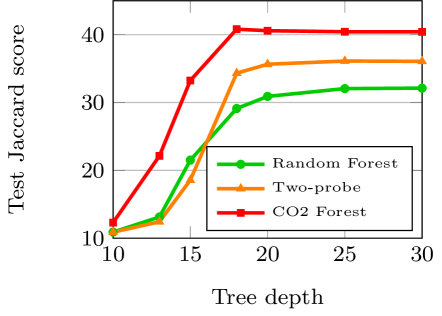
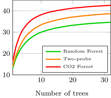
Figure 4: Test Jaccard scores on LFW for (left) forests of $16$ trees with different tree depth constraint from $10$ to $30$ (right) forests with different number of trees from $1$ to $32$.

7 Conclusion

We present Continuously Optimized Oblique (CO2) Forest, a new variant of random forest that uses oblique split functions. Even though the information gain criterion used for inducing decision trees is discontinuous and hard to optimize, we propose a continuous upper bound on the information gain objective. We leverage this bound to optimize oblique decision tree ensembles, which achieve a large improvement on classification benchmarks over a random forest baseline and previous methods of constructing oblique decision trees. In contrast to OC1 trees, our method scales to problems with high-dimensional inputs and large training sets, which are commonplace in Computer Vision and Machine Learning. Our framework is straightforward to generalize to other tasks, such as regression or structured prediction, as the upper bound is general and applies to any form of convex loss function.

References

- [1] http://ccb.jhu.edu/software/oc1/oc1.tar.gz.
- [2] http://www.csie.ntu.edu.tw/~cjlin/libsvmtools/datasets/multiclass.html.
- [3] K. P. Bennett and J. A. Blue. A support vector machine approach to decision trees. IJCNN, 1998.
- [4] L. Breiman. Bagging predictors. Machine learning, 24(2), 1996.
- [5] L. Breiman. Random forests. Machine Learning, 45(1):5–32, 2001.
- [6] L. Breiman, J. Friedman, R. A. Olshen, and C. J. Stone. Classification and regression trees. Chapman & Hall/CRC, 1984.
- [7] A. Criminisi and J. Shotton. Decision Forests for Computer Vision and Medical Image Analysis. Springer, 2013.
- [8] M. Denil, D. Matheson, and N. De Freitas. Narrowing the gap: Random forests in theory and in practice. ICML, 2014.
- [9] P. F. Felzenszwalb, R. B. Girshick, D. McAllester, and D. Ramanan. Object detection with discriminatively trained part-based models. IEEE Trans. PAMI, pages 1627–1645, 2010.
- [10] J. H. Friedman. Greedy function approximation: a gradient boosting machine. Annals of Statistics, pages 1189–1232, 2001.
- [11] T. Hastie, R. Tibshirani, and J. Friedman. The elements of statistical learning (Ed. 2). Springer, 2009.
- [12] D. Heath, S. Kasif, and S. Salzberg. Induction of oblique decision trees. IJCAI, 1993.
- [13] T. K. Ho. The random subspace method for constructing decision forests. IEEE Trans. PAMI, pages 832–844, 1998.
- [14] G. B. Huang, M. Ramesh, T. Berg, and E. Learned-Miller. Labeled faces in the wild: A database for studying face recognition in unconstrained environments. Technical Report 07-49, University of Massachusetts, Amherst, 2007.
- [15] L. Hyafil and R. L. Rivest. Constructing optimal binary decision trees is NP-complete. Information Processing Letters, 5(1):15–17, 1976.
- [16] M. I. Jordan and R. A. Jacobs. Hierarchical mixtures of experts and the EM algorithm. Neural Comput., 6(2):181–214, 1994.
- [17] P. Kontschieder, P. Kohli, J. Shotton, and A. Criminisi. GeoF: Geodesic forests for learning coupled predictors. CVPR, 2013.
- [18] B. H. Menze, B. M. Kelm, D. N. Splitthoff, U. Koethe, and F. A. Hamprecht. On oblique random forests. In Machine Learning and Knowledge Discovery in Databases, pages 453–469. 2011.
- [19] S. K. Murthy, S. Kasif, and S. Salzberg. A system for induction of oblique decision trees. Journal of Artificial Intelligence Research, 1994.
- [20] M. Norouzi and D. J. Fleet. Minimal Loss Hashing for Compact Binary Codes. ICML, 2011.
- [21] M. Norouzi, D. J. Fleet, and R. Salakhutdinov. Hamming Distance Metric Learning. NIPS, 2012.
- [22] S. Nowozin, C. Rother, S. Bagon, T. Sharp, B. Yao, and P. Kohli. Decision tree fields. ICCV, 2011.
- [23] F. Pedregosa, G. Varoquaux, A. Gramfort, V. Michel, B. Thirion, O. Grisel, M. Blondel, P. Prettenhofer, R. Weiss, V. Dubourg, J. Vanderplas, A. Passos, D. Cournapeau, M. Brucher, M. Perrot, and E. Duchesnay. Scikit-learn: Machine learning in Python. JMLR, pages 2825–2830, 2011.
- [24] J. R. Quinlan. Induction of decision trees. Machine learning, 1986.
- [25] J. R. Quinlan. C4.5: programs for machine learning. Elsevier, 1993.
- [26] S. Rota Buló and P. Kontschieder. Neural decision forests for semantic image labelling. CVPR, 2014.
- [27] J. Shotton, R. Girshick, A. Fitzgibbon, T. Sharp, M. Cook, M. Finocchio, R. Moore, P. Kohli, A. Criminisi, A. Kipman, and A. Blake. Efficient human pose estimation from single depth images. IEEE Trans. PAMI, 2013.
- [28] J. Shotton, T. Sharp, P. Kohli, S. Nowozin, J. Winn, and A. Criminisi. Decision jungles: Compact and rich models for classification. In NIPS, pages 234–242. 2013.
- [29] B. M. Smith, L. Zhang, J. Brandt, Z. Lin, and J. Yang. Exemplar-based face parsing. In CVPR, pages 3484–3491, 2013.
- [30] R. Tibshirani and T. Hastie. Margin trees for high-dimensional classification. JMLR, 8, 2007.
- [31] I. Tsochantaridis, T. Hofmann, T. Joachims, and Y. Altun. Support vector machine learning for interdependent and structured output spaces. ICML, 2004.
- [32] C.-N. J. Yu and T. Joachims. Learning structural SVMs with latent variables. ICML, 2009.
- [33] A. L. Yuille and A. Rangarajan. The concave-convex procedure. Neural Comput., pages 915–936, 2003.
- [34] J. Zhu, H. Zou, S. Rosset, and T. Hastie. Multi-class adaboost. Statistics and Its Interface, 2009.