Lord of the Rings: A Kinematic Distance to Circinus X-1 from a Giant X-Ray Light Echo

Abstract

Circinus X-1 exhibited a bright X-ray flare in late 2013. Follow-up observations with Chandra and XMM-Newton from 40 to 80 days after the flare reveal a bright X-ray light echo in the form of four well-defined rings with radii from 5 to 13 arcminutes, growing in radius with time. The large fluence of the flare and the large column density of interstellar dust towards Circinus X-1 make this the largest and brightest set of rings from an X-ray light echo observed to date. By deconvolving the radial intensity profile of the echo with the MAXI X-ray lightcurve of the flare we reconstruct the dust distribution towards Circinus X-1 into four distinct dust concentrations. By comparing the peak in scattering intensity with the peak intensity in CO maps of molecular clouds from the Mopra Southern Galactic Plane CO Survey we identify the two innermost rings with clouds at radial velocity $\sim-74\,{\rm km\,s^{-1}}$ and $\sim-81\,{\rm km\,s^{-1}}$, respectively. We identify a prominent band of foreground photoelectric absorption with a lane of CO gas at $\sim-32\,{\rm km\,s^{-1}}$. From the association of the rings with individual CO clouds we determine the kinematic distance to Circinus X-1 to be $D_{\rm CirX-1}=9.4^{+0.8}_{-1.0}\,{\rm kpc}$. This distance rules out earlier claims of a distance around $4\,{\rm kpc}$, implies that Circinus X-1 is a frequent super-Eddington source, and places a lower limit of $\Gamma\mathrel{\hbox{\hbox to0.0pt{\hbox{\lower 4.0pt\hbox{$\sim$}}\hss}\hbox{$>$}}}22$ on the Lorentz factor and an upper limit of $\theta_{\rm jet}\mathrel{\hbox{\hbox to0.0pt{\hbox{\lower 4.0pt\hbox{$\sim$}}\hss}\hbox{$<$}}}3^{\circ}$ on the jet viewing angle.

1. Introduction

1.1. X-ray Dust Scattering Light Echoes

X-rays from bright point sources are affected by scattering off interstellar dust grains as they travel towards the observer. For sufficiently large dust column densities, a significant fraction of the flux can be scattered into an arcminute-sized, soft X-ray halo. Dust scattering halos have long been used to study the properties of the interstellar medium and, in some cases, to constrain the properties of the X-ray source (e.g. Mathis & Lee, 1991; Predehl & Schmitt, 1995; Corrales & Paerels, 2013).

When the X-ray source is variable, the observable time-delay experienced by the scattered X-ray photons relative to the un-scattered X-rays can provide an even more powerful probe of the ISM than a constant X-ray halo. In this case, the dust scattering halo will show temporal variations in intensity that can be cross-correlated with the light curve to constrain, for example, the distance to the dust clouds along the line-of-sight (e.g., Xiang et al., 2011).

A special situation arises when the X-ray source exhibits a strong and temporally well-defined flare (as observed, for example, in gamma-ray bursts and magnetars). In this case, the scattered X-ray signal is not a temporal and spatial average of the source flux history and the Galactic dust distribution, but a well-defined light echo in the form of distinct rings of X-rays that increase in radius as time passes, given the longer and longer time delays (Vianello et al., 2007).

The scattering geometry of X-rays reflected by an interstellar dust cloud is illustrated in Fig. 1. For a source distance $D$ and a layer of interstellar dust at distance $xD$ from the observer (such that the fractional distance to the dust layer is $x$), the scattered X-rays must travel an additional distance $\Delta D$ which depends on the observed off-axis angle $\theta$ (e.g. Mathis & Lee, 1991; Xiang et al., 2011):

$$\Delta D = xD\left(\frac{1}{\cos({\theta})}-1\right)+\left(1-x\right)D\left(\frac{1}{\cos({\alpha})}-1\right)$$ (1)

$$\approx \frac{xD\theta^{2}+(1-x)D\alpha^{2}}{2}=\frac{xD\theta^{2}}{2\left(1-x\right)}$$

where we have used the small-angle approximation. The scattered signal will arrive with a time delay of

$$\Delta t=\frac{\Delta D}{c}=\frac{xD\theta^{2}}{2c(1-x)}$$ (2)

Figure 1.— Cartoon of dust scattering geometry and nomenclature used throughout this paper. X-rays from a source at distance $D$ scatter off a single dust layer at distance $xD$ (such that the fractional distance is $x$). The observed angle of the scattered X-rays is $\theta$, while the true scattering angle is $\theta_{\rm sc}=\theta+\alpha$. The scattered X-rays travel an additional path length of $\Delta D=\Delta D_{1}+\Delta D_{2}$.

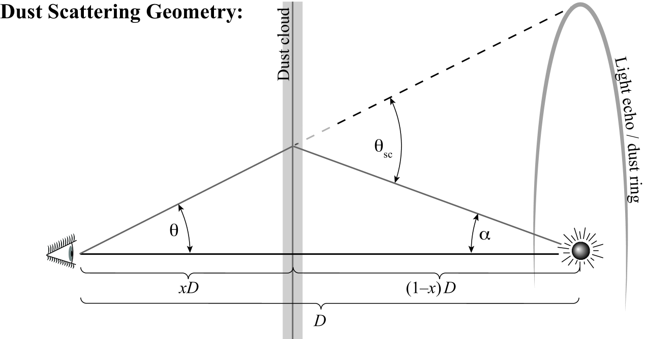
For a well-defined (short) flare of X-rays, the scattered flare signal propagates outward from the source in an annulus of angle

$$\theta=\sqrt{\frac{2c\Delta t(1-x)}{xD}}$$ (3)

For a point source X-ray flux $F(t)$ scattered by a thin sheet of dust of column density $N_{\rm H}$, the X-ray intensity $I_{\nu}$ of the dust scattering annulus at angle $\theta$ observed at time $t_{\rm obs}$ is given by (Mathis & Lee, 1991)

$$I_{\nu}(\theta,t_{\rm obs})=N_{\rm H}\frac{F_{\nu}(t_{\rm obs}-\Delta t_{\theta})}{\left(1-x\right)^{2}}\frac{d\sigma_{\nu}}{d\Omega}$$ (4)

where $\Delta t_{\theta}$ is given by eq. (2) and $d\sigma_{\nu}/d\Omega$ is the differential dust scattering cross section per Hydrogen atom, integrated over the grain size distribution (e.g. Mathis & Lee, 1991; Draine, 2003). In the following, we will refer to the quantity $N_{\rm H}d\sigma_{\nu}/d\Omega$ as the dust scattering depth.

For a flare of finite duration scattering off a dust layer of finite thickness, the scattered signal will consist of a set of rings that reflect the different delay times for the different parts of the lightcurve relative to the time of the observation and the distribution of dust along the line of sight.

In the presence of multiple well-defined scattering layers at different fractional distances $x$ (with thickness $l_{\rm dust}\ll D$), each layer will generate a separate set of annuli. At a given time delay, the annuli of a fixed, short segment of the lightcurve are defined by the intersections of an ellipsoid of constant path length and each scattering layer. The superposition of the annuli from all dust layers (clouds) and the different parts of the flare light curve will create a set of (partially overlapping) rings. This situation is illustrated in Fig. 2.

Figure 2.— Cartoon of the X-ray dust-scattering echo analyzed in this paper: A bright flare from a point source (center of the source plane) propagates towards the observer. Dust in dense interstellar clouds between observer and source scatters X-rays towards the observer, producing a light echo in the form of well defined rings. In this example, four clouds [a]-[d] shown in blue, green, yellow, and red, are located at different distances, illuminated by a bright flare (blue lightcurve) and producing four well defined rings in the image/source plane.

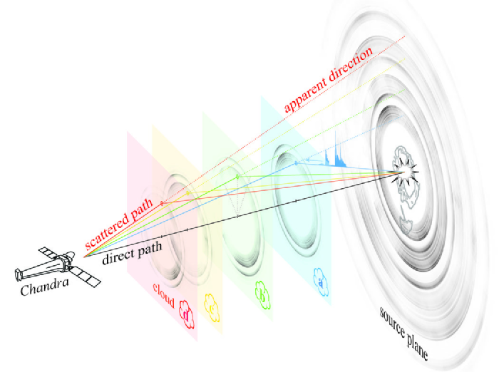
If the lightcurve of the X-ray flare that created the echo is known, an X-ray image of such a set of light-echo rings with sufficiently high angular resolution and signal-to-noise may be de-composed into contributions from a set of distinct dust layers at different distances. Such observations require both high angular resolution and sufficiently large collecting area and low background to detect the rings. The Chandra X-ray observatory is ideally suited for such observations.

1.2. Dust Echoes of Galactic X-ray Sources

X-ray rings generated by dust scattering light echoes are extremely rare. To date, rings have been reported from five gamma-ray bursts (Vianello et al., 2007, and references therein). For Galactic X-ray sources, observations of light echoes have been even more elusive. The soft gamma-ray repeater 1E 1547.0-5408 was the first Galactic X-ray source to show a clear set of bright X-ray light echo rings (Tiengo et al., 2010). Two other sources have also been reported to show light echo rings: the soft gamma-ray repeater SGR 1806-20 (Svirski et al., 2011) and the fast X-ray transient IGR J17544-2619 (Mao et al., 2014). However, the fluence of the initial X-ray flare in the latter two cases was too low to produce clearly resolved, arcminute-scale rings and both detections are tentative. In addition, McCollough et al. (2013) found repeated scattering echoes from a single ISM cloud towards Cygnus X-3.

Figure 3.— MAXI 2-4 keV lightcurve of Circinus X-1 at the time of the 2013 flare. Also shown are the median-times of our two Chandra and three XMM observations (XMM ObsID 0729560701 was not used in this paper). $T_{0}$ was chosen to correspond to the time of our first Chandra observation at ($T_{0}=$MJD₁₅₈₀₁=56683). Red diamond symbols indicate periastron at orbital phase zero (Nicolson, 2007).

In the case of GRBs, the source is known to be at cosmological distances, which makes the scattering geometry particularly simple, since the source is effectively at infinite distance and the scattering angle is equal to the observed ring angle on the sky, which simplifies eq. (3) to

$$\theta_{\rm GRBecho}=\sqrt{\frac{2c\Delta t}{D_{\rm dust}}}$$ (5)

An observed ring radius $\theta_{\rm GRBecho}$ and delay time $\Delta t$ therefore unambiguously determines the distance to the dust.

However, in the case of Galactic sources, eq. (3) for $\theta(\Delta t,D,x)$ cannot be inverted to solve for the distance to either the dust or the source individually, unless the distance to either the source or the dust is known apriori. If a particular ring can be identified with a dust cloud of known distance $xD$, the distance to the source can be determined from the known delay time $\Delta t$.

1.3. Circinus X-1

Circinus X-1 is a highly variable X-ray binary that has often been characterized as erratic. It has been difficult to classify in terms of canonical X-ray binary schemes, combining properties of young and old X-ray binaries (Stewart et al., 1991; Oosterbroek et al., 1995; Jonker et al., 2007; Calvelo et al., 2012). The presence of type I X-ray bursts (Tennant et al., 1986; Linares et al., 2010) identifies the compact object in the source as a neutron star with a low magnetic field, supported by the presence of jets and the lack of X-ray or radio pulses (Stewart et al., 1993; Fender et al., 2004a; Tudose et al., 2006; Heinz et al., 2007; Soleri et al., 2009; Sell et al., 2010).

Figure 4.— Exposure-corrected image of Chandra ObsID 15801, smoothed with a FWHM=10.5” Gaussian. Red: 1-2 keV, green: 2-3 keV, blue: 3-5 keV. Point sources and the read streak produced by Circinus X-1 were removed. Four separate rings of dust scattering echoes are visible in this image.

The transient nature and the low magnetic field suggested a classification of Circinus X-1 as an old, low-mass X-ray binary with an evolved companion star (e.g. Shirey et al., 1996). This interpretation was in conflict with the observed orbital evolution time of order $P/\dot{P}\,\sim\,3,000$ years (Parkinson et al., 2003; Clarkson et al., 2004) to $P/\dot{P}\,\sim\,20,000$ years (Nicolson, 2007) and the possible identification of an A-B type super-giant companion star (Jonker et al., 2007), suggesting a much younger system age and a likely massive companion star. The orbital period of the system is 16.5 days, with a likely eccentricity around 0.45 (Jonker et al., 2007)

The conflicting identifications were resolved with the discovery of an arcminute scale supernova remnant in both X-ray and radio observations (Heinz et al., 2013), placing an upper limit of $\tau<4,600\,{\rm years}\,(D_{\rm Cir}/8\,{\rm kpc})$ on the age of the system, where $D_{\rm Cir}$ is the distance to the source. This upper limit makes Circinus X-1 the youngest known X-ray binary and an important test case for the study of both neutron star formation and orbital evolution in X-ray binaries.

The distance to Circinus X-1 is highly uncertain. As a southern source deeply embedded in the Galactic disk, most standard methods of distance determination are not available. It is also out of the range of VLBI parallax measurements. Distance estimates to Circinus X-1 range from $4\,{\rm kpc}$ (Iaria et al., 2005) to $11\,{\rm kpc}$ (Stewart et al., 1991). A likely range of $D=8-10.5\,{\rm kpc}$ was proposed by Jonker & Nelemans (2004) based on the radius-expansion burst method, using properties of the observed type I X-ray bursts. Because important binary properties depend on the distance to the source (such as the Eddington fraction of the source in outburst), a more accurate determination of the distance is critical for a more complete understanding of this important source.

Circinus X-1 is a highly variable source, spanning over four orders of magnitude in luminosity from its quiescent flux to its brightest flares. While the source was consistently bright during the 1990’s, it underwent a secular decline in flux starting in about 2000 and has spent the past 10 years below the detection thresholds of the Rossi X-ray Timing Explorer All Sky Monitor and the MAXI all sky monitor aboard the International Space Station (Matsuoka et al., 2009), with the exception of sporadic near-Eddington flares, sometimes in excess of one Crab in flux (throughout the paper we will refer to the Eddington limit of $L_{\rm Edd,NS}\sim 1.8\times 10^{38}\,{\rm ergs\,s^{-1}}$ for a $1.4\,{\rm M}_{\odot}$ neutron star). These flares typically occur within individual binary orbits and are characterized by very rapid rises in flux near periastron of the binary orbit and often rapid flux decays at the end of the orbit. For example, during the five years it has been monitored by MAXI, Circinus X-1 exhibited ten binary orbits with peak 2-10 keV fluxes in excess of $\sim 10^{-8}\,{\rm ergs\,cm^{-2}\,s^{-1}}$ and five orbits with peak flux at or above one Crab.

The large dynamic range of the source flux, the well-defined duration of the X-ray flares, and the low mean flux during the quiescent periods over the past decades make Circinus X-1 an ideal source for observations of X-ray light echoes. The source is located in the Galactic plane, at Galactic coordinates $l=322.12^{\circ},b=0.04^{\circ}$. The large neutral hydrogen column density of $N_{\rm H}\sim 2\times 10^{22}\,{\rm cm^{-2}}$, inferred from photo-electric absorption of the X-ray spectra of both the neutron star (e.g. Brandt & Schulz, 2000) and the supernova remnant (Heinz et al., 2013), further increases the likelihood to observe light echoes.

In late 2013, Circinus X-1 underwent an extremely bright flare, preceded and followed by long periods of very low X-ray flux. In this paper, we report the detection of the brightest and largest set of X-ray dust scattering rings observed to date, generated by the light echo from the 2013 flare. The spatial variation of the rings allows us to identify the interstellar clouds responsible for the different rings, which determines the distance to the X-ray source, Circinus X-1, to roughly 10% accuracy.

Figure 5.— Exposure-corrected and background-subtracted image of XMM-Newton ObsID 0729560501 (combining EPIC MOS and PN data), smoothed with a FWHM=35” Gaussian. Colors represent the same energy bands as in Fig. 4. Point sources have been removed. The over-plotted white-dashed line corresponds to the $15{\rm K\,km\,s^{-1}}$ contour of the $-33.6$ to $-29.6\,{\rm km\,s^{-1}}$ ¹²CO image shown in Fig. 19.

We will describe the observations and data analysis in §2. Section 3 describes the analysis of the X-ray, CO, and HI data and the procedure for deconvolving the X-ray signal into the line-of-sight dust distribution. In §4, we derive a new distance to Circinus X-1 and discuss the consequences for the physics of this unique X-ray binary and for the physics of dust scattering. Section 5 briefly summarizes our findings.

2. Observations and Data Reduction

2.1. X-Ray Observations

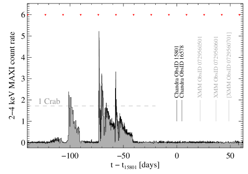
Circinus X-1 was observed with Chandra, XMM-Newton, and Swift in early 2014 after a bright X-ray flare of the source in late 2013. Figure 3 shows the time of the Chandra and XMM-Newton observations overlaid on the MAXI lightcurve of the source. The source exhibited a bright flare during three binary orbits approximately 50 to 100 days before the first Chandra observation (Asai et al., 2014), with a quiescent binary orbit interspersed during the first half of the flare. The source flare reached fluxes in excess of one Crab, with a total 2-4 keV fluence of ${\mathcal{F}}_{2-4}=0.025\,{\rm ergs\,cm^{-2}}$. The lightcurve of the flare has three characteristic peaks and a pronounced gap. This is the most energetic flare Circinus X-1 exhibited since it entered its long-term quiescent state in 2006, and is comparable in peak flux to the brightest flares the source has undergone even during its long-term outburst.

Before and during the Chandra campaign, Swift observed the source twelve times for a total exposure of 12 ksec in order to safely schedule the Chandra observations. The history of bright flares by Circinus X-1, which can exceed the ACIS dose limit even during moderate exposures presents a significant scheduling challenge, and frequent monitoring of the source with Swift was used to confirm that the source was safely below the maximum flux allowable under Chandra instrument safety rules. The short total exposure time and the fact that the exposures were spread over a time window of 11 days make the Swift data unsuitable for the analysis presented in this paper.

Figure 6.— Un-absorbed 2-5 keV scattering intensity in units of $10^{-7}\,{\rm ergs\,cm^{-2}\,s^{-1}\,Sr^{-1}}$ across the Chandra field-of-view, derived from spectral fits to Chandra ObsID 15801 on a rectangular grid of 8$\times$8 squares per CCD, labeled by row and column from 1 through 24 and A through P, respectively. Photo-electric absorption was removed to isolate the dust-scattered intensity.

2.1.1 Chandra Observations

In the 3.5 binary orbits preceding the first Chandra observation, as well as during the months prior to the flare, the source was quiescent, below the MAXI detection threshold. We observed the source on two occasions with Chandra, on January 25, 2014 for 125 ksec, and on January 31, 2014 for 55 ksec, listed as ObsID 15801 and 16578, respectively. The point source was at very low flux levels during both observations. Circinus X-1 was placed on the ACIS S3 chip.

Data were pipeline processed using CIAO software version 4.6.2. Point sources were identified using the wavdetect (Freeman et al., 2002) task and ObsID 16578 was reprojected to match the astrometry of ObsID 15801. For comparison and analysis purposes, we also reprocessed ObsID 10062 (2009) with CIAO 4.6.2 and reprojected it to match the astrometry of ObsID 15801.

We prepared blank background images following the standard CIAO thread (see also Hickox & Markevitch, 2006), matching the hard ($>$10 keV) X-ray spectrum of the background file for each chip.

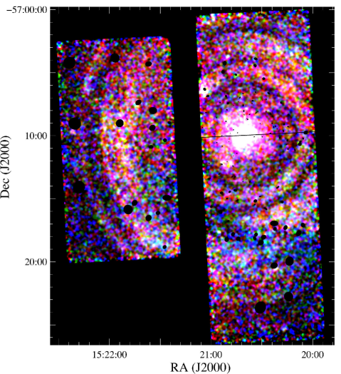
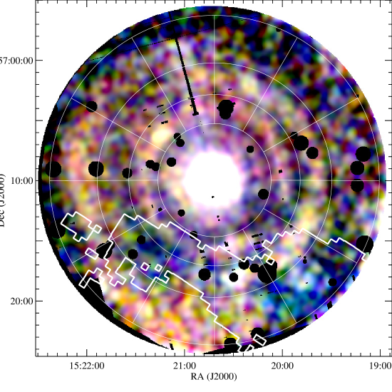
Figure 4 shows an exposure-corrected, background-subtracted three-color image of the full ACIS field-of view captured by the observation (ACIS chips 2,3,6,7, and 8 were active during the observation), where red, green, and blue correspond to the 1-2, 2-3, and 3-5 keV bands, respectively. Point sources were identified using wavdetect in ObsIDs 10062, 15801, and 16578, source lists were merged and point sources were removed from imaging and spectral analysis. The read streak was removed and the image was smoothed with a 10.5” full-width-half-max (FWHM) Gaussian in all three bands.

The image shows the X-ray binary point source, the X-ray jets (both over-exposed in the center of the image), and the supernova remnant in the central part of the image around the source position at 15:20:40.9,-57:10:00.1 (J2000).

The image also clearly shows at least three bright rings that are concentric on the point source. The first ring spans from 4.2 to 5.7 arcminutes in radius, the second ring from 6.1 to 8.2 arcminutes, and the third from 8.3 to 11.4 arcminutes in radius, predominantly covered by the Eastern chips 2 and 3. We will refer to these rings as rings [a], [b], and [c] from the inside out, respectively. An additional ring-like excess is visible at approximately 13 arcminutes in radius, which we will refer to as ring [d].

As we will lay out in detail in §4, we interpret these rings as the dust-scattering echo from the bright flare in Oct.-Dec. of 2013, with each ring corresponding to a distinct concentration of dust along the line-of-sight to Circinus X-1. A continuous dust distribution would not produce the distinct, sharp set of rings observed by Chandra.

Figure 7.— Distribution of photo-electric absorption column $N_{\rm H}$ derived from the spectral fits shown in Fig. 6. A clear excess of absorption is found in the lower half of the image. Over-plotted is the $15\,{\rm K\,km\,s^{-1}}$ contour of the $-33.6$ to $-29.6\,{\rm km\,s^{-1}}$ ¹²CO image shown in Fig. 19.

The rings are also clearly visible in ObsID 16578, despite the shorter exposure and the resulting lower signal-to-noise. In ObsID 16578, the rings appear at $\sim$4% larger radii, consistent with the expectation of a dust echo moving outward in radius [see also §3.2 and eq. (10)]. The rings are easily discernible by eye in the energy bands from 1 to 5 keV.

Even though the outer rings are not fully covered by the Chandra field of view (abbreviated as FOV in the following), it is clear that the rings are not uniform in brightness as a function of azimuthal angle. There are clear intensity peaks at [15:21:00,-57:06:30] in the inner ring [a] and at [15:20:20,-57:16:00] in ring [b] of ObsID 15801. Generally, ring [c] appears brighter on theSouth- Eastern side of the image.

The deviation from axi-symmetry observed here differs from almost all other observations of dust scattering signatures, which typically appear to be very uniform in azimuth. For example, a detailed investigation of the dust scattering halo of Cygnus X-2 found that the profile deviated by only about 2% from axi-symmetry (Seward & Smith, 2013). The only comparable observational signature of non-symmetric scattering features is the light echo off a bok globule observed for Cygnus X-3 (McCollough et al., 2013)

In addition to the light echo, a blue ”lane” is visible across the lower part of the image. As we will show below, this feature is the result of photoelectric foreground absorption by an additional layer of dust and gas closer to the observer than the clouds producing the light echo.

2.1.2 XMM-Newton Observations

XMM-Newton observed the source on 17 February, 2014 (ObsID 0729560501), 4 March, 2014 (ObsID 0729560601), and 16 March, 2014 (ObsID 0729560701) for 30 ksec each. ObsID 0729560501 was not affected by any background flares. The second and third observation were strongly affected by background particle flares, eliminating the use of PN data completely for ObsID 0729560601, and the effective exposure for the MOS detectors after flare rejection was cut to approximately 15ksec in both cases. The resulting data are noisy, suggesting that additional background contamination is present, making the data not usable for detailed, quantitative image processing. We restrict the discussion in this paper to data set 0729560501 (with the exception of Fig. 15).

Figure 8.— Un-absorbed excess 2-5 keV scattering intensity in units of ${\rm ergs\,cm^{-2}\,s^{-1}\,Sr^{-1}}$ across the XMM field-of-view, derived from spectral fits in annular sections identical to those plotted in Fig. 5. Photo-electric absorption was removed to isolate the dust-scattered intensity. Clear peaks in the surface brightness are located ring sections section [a11] and [b6].

MOS and PN data were reduced using SAS software version 13.5. Data were prepared using the ESAS package, following the standard diffuse source analysis guidelines from the Diffuse Analysis Cookbook. In addition to point sources identified by the ESAS cheese task, point sources identified in the three Chandra exposures (10062, 15801, 16578) were removed before image and spectral extraction. The energy range from 1.4-1.6 keV around the prominent instrumental Aluminum line at 1.5 keV was removed from image processing, while spectral fits determined that the contribution from the Si line at 1.75 keV was sufficiently small to ignore in image processing. Proton and solar-wind charge exchange maps were created using spectral fits to the outer regions of the image and subtracted during image processing.

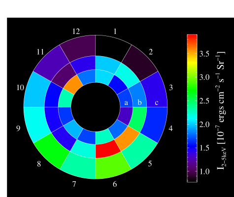
Figure 5 shows a three color exposure-corrected image of ObsID 0729560501 in the same bands as Fig. 4, smoothed with a 35” FWHM Gaussian. Despite the lower spatial resolution of XMM-Newton, the image clearly shows the three rings identified in the Chandra images. The median radii of the rings have increased by $\sim$16% relative to ObsID 15801, corresponding to the longer time delay between the flare and the XMM observation.

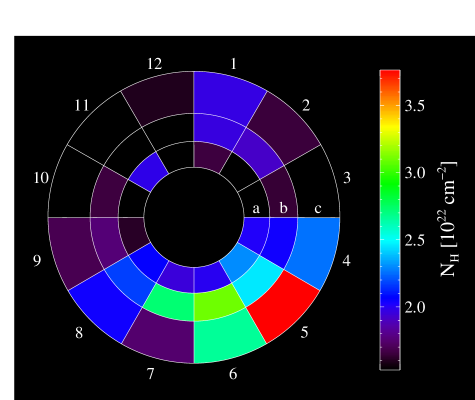
Overlaid on the figure is a grid of three annuli covering the rings, broken into twelve angular sections of 30^∘ each. We will use this grid in the discussion below to identify different areas in the image and in corresponding CO maps of the FOV. The rings are labeled [a],[b], and [c] from inside out, and the sections are labeled 1-12 in a clock-wise fashion. See §3.1 and Fig. 8 for further details on the grid and the nomenclature used in this paper.

2.2. CO Data

We used CO data from the Mopra Southern Galactic Plane CO Survey, described in Burton et al. 2013, with the particular data set used here, for the Circinus X-1 region (l=322°), coming from the forthcoming public data release in Braiding et al., 2015 (in preparation). In this data set emission from the J=1-0 line of the three principal isotopologues of the CO molecule (¹²CO, ¹³CO, C¹⁸O, at 115.27, 110.20 and 109.78 GHz, respectively) has been measured at 0.6 arcmin, $0.1\,{\rm km\,s^{-1}}$ resolution with the 22m diameter Mopra millimetre wave telescope, located by Siding Spring Observatory in New South Wales in Australia.

Figure 9.— Distribution of photo-electric absorption column $N_{\rm H}$ derived from the spectral fits shown in Fig. 8. A clear excess of absorption is found in the lower half of the image, with a peak at position [c5].

By continuously scanning the telescope while making the observations (on-the-fly mapping) large areas of sky can be readily mapped by Mopra. Data cubes covering $1^{\circ}\times 1^{\circ}$ of sky typically take 4 nights with the telescope to obtain, and achieve a 1 sigma sensitivity of about 1.3K and 0.5K per $0.1\,{\rm km\,s^{-1}}$ velocity channel for the 12CO and the (13CO, C18O) lines, respectively. Such a data cube, covering the G322 region ($l=322^{\circ}-323^{\circ}$, $b=-0.5^{\circ}$ to $+0.5^{\circ}$), was used for the analysis presented here.

2.3. 21 cm Data

We use publicly available 21 cm radio data from the Parkes/ATCA Southern Galactic Plane survey (McClure-Griffiths et al., 2005) to estimate the column density of neutral atomic hydrogen towards Circinus X-1. We use CO data to identify velocity components because the velocity dispersion of the HI velocity components is too large to unambiguously resolve individual clouds.

3. Analysis

3.1. X-ray Spectral Fits

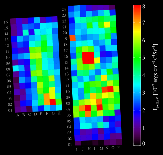
We performed spectral fits of data from Chandra ObsID 15801 and XMM ObsID 0729560501, with results from the spectral analysis presented in Figs. 6-9. Because the XMM-Newton FOV is contiguous and covers the rings entirely, we extracted spectra for each ring of XMM ObsID 0729560501 in annuli spanning the radial ranges [4.7’-7.1’,7.1’-9.7’,9.7’-13.7’], with each ring divided into twelve sections. Rings are labeled [a] through [c] (with lower case letters denoting XMM rings), and the layout of the grid is shown in Fig. 8. We divided the Chandra FOV into a rectangular grid, with each CCD covered by an 8x8 grid of square apertures. The layout of the grid on the ACIS focal plane is shown in Fig. 6, with columns running from [A] through [P] and rows from 1 to 24 (with capital letters denoting Chandra columns).

Spectra for Chandra ObsID 15801 were generated using the specextract script after point source removal. Background spectra were generated from the blank sky background files. No additional background model was required in fitting the Chandra data, given the accurate representation of the background in the black sky data.

Spectra for XMM-Newton ObsID 0729560501 were extracted from the XMM-MOS data using the ESAS package and following the Diffuse Analysis Cookbook. In spectral fitting of the XMM data, we modeled instrumental features (Al and Si) and solar-wind charge exchange emission by Gaussians with line energies and intensities tied across all spectra and line widths frozen below the spectral resolution limit of XMM-MOS at $\sigma=1\,{\rm eV}$. We modeled the sky background emission as a sum of an absorbed APEC model and an absorbed powerlaw. Intensities of both background components were tied across all ring sections.

We modeled the dust scattering emission in each region as an absorbed powerlaw, with floating absorption column and normalization, but with powerlaw index tied across all regions, with the exception of the tiles covering the central source and the supernova remnant in the Chandra image, which span a square aperture from positon [J14] to [M18]. Tying the powerlaw photon index $\Gamma$ across all spectra is appropriate because (a) the scattering angle varies only moderately across the rings, with

$$\theta_{\rm sc}=\sqrt{\frac{2c\Delta t}{\left(1-x\right)xD}}$$ (6)

and (b) for the scattering angles considered here ($\theta_{\rm sc}>10^{\prime}$), the energy dependence of the scattering cross section is independent of $\theta_{\rm sc}$, with $d\sigma/d\Omega\propto E^{-2}$ (e.g. Draine, 2003). While the source spectrum might have varied during the outburst, we are integrating over sufficiently large apertures to average over possible spectral variations.

Figure 10.— Radial X-ray intensity profile of Chandra ObsID 15801 in the 2-5keV band (chosen to roughly match the MAXI 2-4 keV band), shown in black. The intensity profile of Chandra ObsID 10062 was subtracted to remove the supernova remnant and residual quiescent background. Overlaid is the full reconstructed radial intensity profile from the deconvolution (gray), as well as the contributions from the four distinct dust concentrations along the line of sight identified in Fig. 12 and the powerlaw model of the diffuse instantaneous dust scattering halo (purple line). The hatched area shows the region where the deconvolution becomes unreliable because part of the kernel falls outside of the Chandra FOV or onto the supernova remnant. Top right insert: Dust scattering kernel $K(\theta/\theta_{\rm med})$ [see eq. (9)] used for the deconvolution, derived from the MAXI 2-4 keV lightcurve during the flare shown in Fig. 3, normalized by the total fluence of the outburst.

While the source spectrum during outburst (the echo of which we are observing in the rings) was likely more complicated than a simple powerlaw, we have no direct measurement of the detailed flare spectrum and the quality of the spectra does not warrant additional complications, such as the addition of emission lines which are often present in the spectra when the source is bright (Brandt & Schulz, 2000). Dust scattering is expected to steepen the source spectrum by $\Delta\Gamma=2$, and the measured powerlaw index of

$$\Gamma=4.00\pm 0.03$$ (7)

for the scattered emission is consistent with the typically soft spectrum of $\Gamma\sim 2$ the source displays when in outburst.

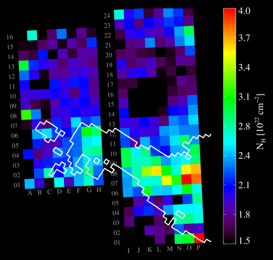
The spectral fits resulting from the model are statistically satisfactory, with a reduced chisquare of $\chi^{2}_{\rm red,0729560501}=839.68/807\,{\rm d.o.f.}=1.04$ for the combined fit of the entire set of spectra for ObsID 0729560501 and $\chi^{2}_{\rm red,15801}=839.68/807\,{\rm d.o.f.}=1.05$ for ObsID 15801. We display the unabsorbed 2-5keV intensity maps of Chandra ObsID 15801 and XMM ObsID 0729560501 in Figs. 6 and 8, respectively. The unabsorbed intensity provides a direct measure of the scattering intensity (unaffected by effects of foreground absorption) and is directly proportional to the dust scattering depth. In Figs. 7 and 9, we show maps of the photo-electric absorption column density $N_{\rm H}$ determined from the spectral fits for Chandra ObsID 15801 and XMM ObsID 0729560501, respectively.

Four properties of the spectral maps stand out that confirm the qualitative description of the color images in Figs. 4 and 5:

1. A clear intensity peak at position [a11] in Fig. 8 and [I19] in Fig. 6 corresponds to the brightness peaks seen at that position in Figs. 4 and 5. The intensity is a factor of two larger than in the neighboring section [a12] in Fig. 8, with a similar increment relative to the neighboring sections in Fig. 6.

2. There is a clear intensity peak at position [b5] and [b6], with [b6] being approximately two times brighter than neighboring [b7] in Fig. 8. Ring [b] is brighter on the Western side of the XMM FOV. This peak of ring [b] corresponds to the brightness peak in tiles [L9], [N10], and [O10] in Fig. 6.

3. The Southern section of ring [c] is brighter than the Northern section, with the brightest scattering emission in sections [c5:c8] in Fig. 8. Ring [d] overlaps significantly with ring [c], and the color images and intensity maps cannot distinguish the angular distribution of the two rings.

4. There is a clear excess of foreground absorption in the Southern sections of the FOV, running from tile [P7] to [B6] in Fig. 7. Figure 9 shows the strongest absorption in sections [c5], [b6] and [b7]. This corresponds to the blue absorption lane that runs across the color images in Figs. 4 and 5.

The rings clearly deviate from axial symmetry about Circinus X-1, which requires a strong variation in the scattering dust column density across the image. Because the rings are well-defined, sharp features, each ring requires the presence of a spatially well separated, thin distribution of dust (where thin means that the extent of the dust sheet responsible for each ring is significantly smaller than the distance to the source, by at least an order of magnitude).

We present a quantitative analysis of the dust distribution derived from the rings in 3.2, but from simple consideration of the images and spectral maps alone, it is clear that the different dust clouds responsible for the rings have different spatial distributions and cannot be uniform across the XMM and Chandra FOVs. In particular, the peak of the cloud that produced the innermost ring (ring [a]) must have a strong column density peak in section [a11], while the cloud producing ring [b] must show a strong peak in sections [b5] and [b6]. The excess of photo-electric absorption in the lower half of the image, with a lane of absorption running through the sections [c5], [b6], and [b7], requires a significant amount of foreground dust and gas (an excess column of approximately $N_{\rm H}\sim 10^{22}\,{\rm cm^{-2}}$ relative to the rest of the field).

3.2. X-ray Intensity Profiles and Dust Distributions

3.2.1 Radial intensity profiles

In order to determine quantitatively the dust distribution along the line of sight, we extracted radial intensity profiles of Chandra ObsID 10062, 15801, and 16578 in 600 logarithmic radial bins from 1’ to 18’.5 in the energy bands 1-2 keV, 2-3 keV, and 3-5 keV (after background subtraction and point-source/read-streak removal). We extracted the radial profile of XMM ObsID 0729560501 in 300 logarithmic bins over the same range in angles. We subtracted the quiescent radial intensity profile of ObsID 10062 to remove the emission by the supernova remnant and residual background emission.

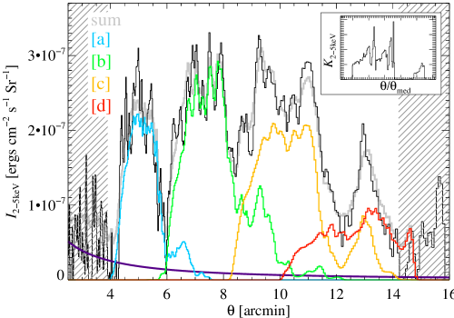
Because of the variation in photo-electric absorption across the field, we restricted analysis to the 2-5 keV band, which is only moderately affected by absorption. We plot the resulting radial intensity profile of Chandra ObsID 15801 in Fig. 10. The plot in Fig. 10 shows four echo rings labeled [a] through [d] which correspond to the visually identified rings in the previous sections. Several bright sharp peaks in $I_{2-5{\rm keV}}(\theta)$ are visible that can also be seen as distinct sharp rings in Fig. 4, suggesting very localized dust concentrations. For comparison, the radial profile of XMM ObsID 0729560501 is plotted in Fig. 11.

3.2.2 Modeling and removing the diffuse instantaneous dust scattering halo

In general, the dust scattering ring echo will be super-imposed on the lower-level instantaneous diffuse dust scattering halo produced by the (weak) emission of the point source during and just prior to the observation, which should be removed before analysis of the echo. The 2-5 keV point source flux during and before ObsID 15801 was very low ($F_{2-5\,{\rm keV,15801}}\mathrel{\hbox{\hbox to0.0pt{\hbox{\lower 4.0pt\hbox{$\sim$}}\hss}\hbox{$<$}}}6\times 10^{-12}\,{\rm erg\,s^{-1}\,cm^{-2}}$), resulting in essentially negligible halo emission, while the two later observations showed larger point source flux ($F_{2-5\,{\rm keV}}\sim 1.8\times 10^{-11}\,{\rm ergs\,s^{-1}\,cm^{-2}}$ for ObsID 16578 and $F\sim 1.3\times 10^{-11}\,{\rm ergs\,s^{-1}\,cm^{-2}}$ for 0729560501, with correspondingly brighter diffuse halo emission).

We model the instantaneous dust scattering halo as a powerlaw in ring angle, $I_{\rm halo}\propto\theta^{\eta}$, appropriate for the large halo angles under consideration and consistent with the steady dust scattering halo profile for Circinus X-1 derived from Chandra ObsID 706 in Heinz et al. (2013).

We determine the powerlaw index to be $\eta\sim-1.5$ by fitting the intensity profile of ObsID 0729560501 in the radial range between the edge of the supernova remnant at $\theta>2.5^{\prime}$ and the inner edge of ring [a] at $\theta<5^{\prime}$. This value of $\eta$ is consistent with the reference dust scattering halo of ObsID 706 from Heinz et al. (2013), which has an index of $\eta\sim-1.55$ in the 2-5 keV band.

Figure 11.— Radial X-ray intensity profile of XMM ObsID 0729560501 in the 2-5keV band, following the same labeling and convention as Fig. 10. The purple line shows the best fit powerlaw profile for the instantaneous dust scattering halo (removed before the deconvolution), the colored lines show the contributions from rings [a]-[d] derived from the radial deconvolution of the profile. Overplotted as dashed lines are the radial profiles from rings [a]-[d] predicted by the deconvolution of the Chandra ObsID 15801 radial profile. Top right insert: Dust scattering kernel $K(\theta/\theta_{\rm med})$ [see eq. (9)] used for the deconvolution.

We determine the powerlaw normalization for ObsID 15801 and 16578 by fits to each radial profile between the outer edge of the remnant at $\theta>2.5^{\prime}$ and the inner edge of ring [a] at $\theta<4^{\prime}$. We overplot the powerlaw fits to the instantaneous halo as purple lines in Fig. 10 and 11. We subtract the halo emission before further analysis of the ring echo in §3.2.4 and §3.2.5.

3.2.3 Deriving the dust distribution

Given the well-sampled MAXI lightcurve of the 2013 flare, we can construct the light echo intensity profile that would be produced by a thin sheet of dust at a given relative dust distance $x$ and observing time $t_{\rm obs}$ from eqs. (3) and (4). In general, the different parts of the flare will generate emission at different radii (echoes of earlier emission will appear at larger angles $\theta$).

The scattering angle and thus the scattering cross section will vary for different parts of the lightcurve, which must be modeled. Given the large scattering angles of $\theta_{\rm sc}\mathrel{\hbox{\hbox to0.0pt{\hbox{\lower 4.0pt\hbox{$\sim$}}\hss}\hbox{$>$}}}1400^{\prime\prime}$ of the rings and photon energies above 2 keV, it is safe to assume that the cross section is in the large angle limit where $d\sigma/d\Omega\propto\theta_{\rm sc}^{-\alpha}\propto\theta^{-\alpha}$ with $\alpha\sim 4$ (Draine, 2003), which we will use in the following. The exact value of $\alpha$ depends on the unknown grain size distribution. By repeating the analysis process with different values of $\alpha$, ranging from 3 to 5, we have verified that our results (in particular, the location of the dust clouds and the distance to Circinus X-1) are not sensitive to the exact value of $\alpha$.

For a thin scattering sheet at fractional distance $x$, the median ring angle $\theta_{\rm med}$ (i.e., the observed angle $\theta$ for the median time delay $\Delta t_{\rm med}$ of the flare) is

$$\theta_{\rm med}=\sqrt{\frac{2c\Delta t_{\rm med}(1-x)}{xD}}$$ (8)

where $\Delta t_{\rm med}$ is a constant set only by the date of the observation and the date range of the flare. The invariant intensity profile $K_{2-5{\rm keV}}$ produced by that sheet depends on the observed angle $\theta$ only through the dimensionless ratio $z\equiv\theta/\theta_{\rm med}$:

$$K_{2-5{\rm keV}}\left(z,x\right)$$

$$= F_{\rm MAXI}(\Delta t_{\rm med}z^{2})\frac{N_{\rm H,x}}{(1-x)^{2}}\left.\frac{d\sigma}{d\Omega}\right|_{\rm\theta=\theta_{\rm med}}z^{-4}$$ (9)

We can therefore decompose the observed radial profile into a series of these contributions from scattering sheets along the line of sight, each of the form $K_{2-5{\rm keV}}(\theta/\theta_{\rm med})$. Because we chose logarithmic radial bins for the intensity profile, we can achieve this by a simple deconvolution of $I_{2-5{\rm keV}}$ with the kernel $K_{2-5{\rm keV}}$. The inset in Fig. 10 shows $K(\theta/\theta_{\rm med})$ for $\alpha=4$.

3.2.4 Deconvolution of the Chandra radial profiles

To derive the dust distribution that gave rise to the light echo, we performed a maximum likelihood deconvolution of the Chandra radial profiles with this kernel into a set of 600 dust scattering screens along the line of sight. We used the Lucy-Richardson deconvolution algorithm (Richardson, 1972; Lucy, 1974) implemented in the IDL ASTROLIB library. In the region of interest (where the scattering profile is not affected by the chip edge and the supernova remnant), the radial bins are larger than the 50% enclosed energy width of the Chandra point spread function (PSF), such that the emission inside each radial bin is resolved.

Figure 10 shows the reconstructed intensity profile from this distribution for ObsID 15801 (derived by re-convolving the deconvolution with $K_{\rm 2-5\,{\rm keV}}$ and adding it to the powerlaw profile for the instantaneous dust scattering halo), which reproduces the observed intensity profile very well, with only minor deviations primarily for rings [a] from 4’-6’, while the profile outward of 6’ is matched to within the statistical uncertainties.

Figure 12.— Maximum likelihood deconvolution of the 2-5 keV radial intensity profile shown in Fig. 10, plotted as a histogram of scattering depth along the line of sight (rebinned onto a uniform grid in $\theta$). Shown in color (left-hand y-axis) is the invariant effective scattering depth $(1-x)^{-2}N_{\rm H}d\sigma/d\Omega$, where $x$ is the fractional distance of the dust sheet relative to the distance to Circinus X-1 and $d\sigma/d\Omega$ is the scattering cross section evaluated at the mean scattering angle of the sheet and at 2 keV. The distribution shows four main components (labeled [a]-[d] in colors blue, green, yellow, and red, respectively). Also shown in gray is the inferred absolute scattering depth $N_{\rm H}d\sigma/d\Omega$ for the best fit distance of $D_{\rm CirX-1}=9.4{\rm kpc}$ (right-hand y-axis), along with the absolute distance to the scatterer and the associated radial velocity due to Galactic rotation (top axes in gray).

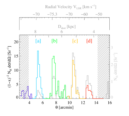
In Fig. 12, we plot the inferred dust distribution along the line of sight as a function of median ring angle $\theta_{\rm med}$, derived from our deconvolution of the intensity profile of ObsID 15801, and rebinned onto a uniform grid in $\theta$. The plotted quantity is a histogram of the invariant differential scattering depth $N_{\rm H}(1-x)^{2}\left.d\sigma/d\Omega\right|_{\theta=\theta_{\rm med}}$ per bin, which is independent of the distance to Circinus X-1.

Table 1Gaussian fits to dust clouds identified in the radial deconvolution in Fig. 12

Ring:	$\theta_{\rm med}$	$\sigma_{\theta}$	$\frac{N_{\rm H}}{(1-x)^{2}}\frac{d\sigma}{d\Omega}[Sr^{-1}]$	$x$
Chandra ObsID 15801
[a]	$5.37^{\prime}\pm 0.02^{\prime}$	$0.21^{\prime}\pm 0.02^{\prime}$	$52.56\pm 7.62$	$0.83$
[b]	$7.63^{\prime}\pm 0.01^{\prime}$	$0.19^{\prime}\pm 0.01^{\prime}$	$47.86\pm 4.77$	$0.70$
[c]	$10.64^{\prime}\pm 0.01^{\prime}$	$0.22^{\prime}\pm 0.01^{\prime}$	$42.09\pm 3.62$	$0.55$
[d]	$12.85^{\prime}\pm 0.04^{\prime}$	$0.34^{\prime}\pm 0.04^{\prime}$	$19.60\pm 3.17$	$0.45$
Chandra ObsID 16578
[a]	$5.50^{\prime}\pm 0.02^{\prime}$	$0.15^{\prime}\pm 0.02^{\prime}$	$30.25\pm 6.03$	$0.83$
[b]	$7.91^{\prime}\pm 0.02^{\prime}$	$0.20^{\prime}\pm 0.02^{\prime}$	$36.16\pm 4.18$	$0.70$
[c]	$11.10^{\prime}\pm 0.02^{\prime}$	$0.26^{\prime}\pm 0.02^{\prime}$	$39.43\pm 3.29$	$0.55$
[d]	$13.49^{\prime}\pm 0.02^{\prime}$	$0.10^{\prime}\pm 0.02^{\prime}$	$6.51\pm 1.68$	$0.45$
XMM ObsID 0729560501
[a]	$6.00^{\prime}\pm 0.05^{\prime}$	$0.90^{\prime}\pm 0.06^{\prime}$	$29.31\pm 2.32$	$0.84$
[b]	$8.72^{\prime}\pm 0.02^{\prime}$	$0.52^{\prime}\pm 0.02^{\prime}$	$25.56\pm 1.06$	$0.71$
[c]	$12.04^{\prime}\pm 0.02^{\prime}$	$0.73^{\prime}\pm 0.02^{\prime}$	$23.54\pm 0.92$	$0.56$

Note. — Cloud centroids correspond to the median time delay of $\Delta t_{15801}=5.628\times 10^{6}\,{\rm s}$, $\Delta t_{16578}=6.203\times 10^{6}\,{\rm s}$, and $\Delta t_{0729560501}=7.925\times 10^{6}\,{\rm s}$ for ObsID 15801, 16578, and 0729560501, respectively. We do not include ring [d] for XMM ObsID 0729560501 because its centroid falls outside of the MOS FOV.

The dust distribution clearly shows four main dust concentrations toward Circinus X-1, which we plotted in different colors for clarity. We fit each dust component with a Gaussian to determine the mean location and width, with fit values listed in Table 1. Given the longer median time delay for ObsID 16578, the rings should be observed at larger median angles by a factor of

$$\frac{\theta_{\rm med,16578}}{\theta_{\rm med,15801}}=\sqrt{\frac{\Delta t_{\rm med,16578}}{\Delta t_{\rm med,15801}}}=\sqrt{\frac{6.084\times 10^{6}\,{\rm s}}{5.628\times 10^{6}\,{\rm s}}}=1.04$$ (10)

or 4%, which is consistent with the observed increase in $\theta_{\rm ring,med}$, within the typical width of each cloud.

We label the identified dust clouds as components [a], [b], [c], and [d] (plotted in green, blue, yellow, and red, respectively) according to the naming convention adopted above, and identify them with the main X-ray rings seen in the images. To show that this identification is appropriate, we overplot the contribution of each dust cloud to the total intensity profile in the associated color in Fig. 10. Rings [a] and [b] are produced primarily by scattering from clouds [a] and [b], while ring [c] and [d] overlap significantly and contain contributions from both clouds.

We tested the uniqueness of the deconvolution procedure using synthetic radial profiles and verified that the procedure faithfully reproduces the dust profile for randomly placed clouds down to a mean flux of about 50% of the background, for counts rates similar to the ones observed in Chandra ObsID 15801. Thus, while we cannot rule out the presence of additional weak dust rings below the detection threshold, the identification of the four main dust concentrations producing rings [a]-[d] is robust.

3.2.5 Deconvolution of the XMM radial profile

The XMM data are noisier due to (a) the shorter exposure, (b) the lower scattering intensity given the increased scattering angle at the correspondingly longer time delay, (c) the larger background intensity that is more difficult to model than the stable Chandra background, and (d) the brighter dust scattering halo due to the increased point source flux during ObsID 0729560501.

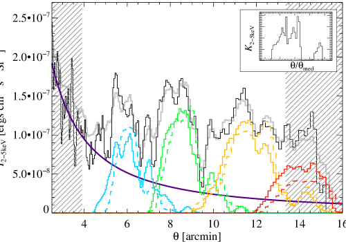
Despite the lower spatial resolution and significantly lower signal-to-noise ratio of the data, the rings are still discernible in the radial profile in Fig. 11. We deconvolved the residual intensity profile following the same procedure used for the Chandra data While the 300 logarithmic radial bins used for the deconvolution are narrower than the 50% enclosed energy width of XMM, we verified that the deconvolution was robust by confirming that a strongly smoothed radial intensity profile and/or a smoothed kernel lead to consistent locations and scattering depths within the measurement uncertainties for the dust screens responsible for rings [a]-[c].. The resulting contributions of rings [a] through [d] are overplotted in color in Fig. 11, following the same convention as Fig. 10.

Gaussian fits to rings [a], [b], and [c] are listed in Table 1. We do not include the fits for ring [d] because its centroid falls too close to the edge of the FOV of XMM-MOS at $\theta\sim 14^{\prime}.5$ (the XMM-PN FOV extends slightly further but is too noisy by itself to reliably extend the profile outward). The inferred relative dust distances agree with the Chandra values to better than 5%, indicating that the deconvolution is robust, and consistent with an increase in median ring radius from Chandra ObsID 15801 to XMM ObsID 0729560501 of $\sim 16$%.

As an additional consistency check, we constructed the radial intensity profile predicted by the deconvolution of the Chandra ObsID 15801 radial profile for the increased time delay of XMM ObsID 0729560501 (including a decrease in surface brightness by a factor of 1.8 due to the $\sim 16\%$ larger scattering angle, assuming $\alpha=4$). The predicted profiles for all four rings are plotted as dashed lines in Fig. 11. The profiles of rings [a]-[c] agree well with the XMM deconvolution, given (a) the different coverage of the FOV by the Chandra and XMM instruments, which should result in moderate differences between the two data sets even if they had been taken at the same time delay and (b) the different angular resolutions and the responses of the telescopes.

3.3. CO Spectral and Image Analysis

The deconvolution into dust sheets from §3.2 shows that the scattering column density must be concentrated in dense, well localized clouds. Gas with sufficiently high column density (of order $10^{21}\,{\rm cm^{-2}}$) and volume number density (of order $100\,{\rm cm^{-3}}$) to produce the observed brightness and arcminute-scale variations in the echo can be expected to be largely in the molecular phase (e.g. Lee et al., 2014).

Figure 13.— Top panel: Radial velocity as a function of distance from the Sun for the sight-line in the direction of Circinus X-1 at Galactic coordinates $l=322.12^{\circ},b=0^{\circ}$, using the rotation curves from McClure-Griffiths & Dickey (2007) and Brand & Blitz (1993) for the inner and outer Galaxy, respectively. Overplotted are the locations and radial velocities for the four dust clouds [a]-[d] (from top to bottom) responsible for the dust scattering rings, assuming the best fit distance of 9.4 kpc. Middle panel: 21cm HI spectrum integrated over rings [a]-[c] defined in Fig.8. Component 1_HI comprises CO components 1_CO and 2_CO listed below. Bottom panel: ¹²CO spectrum integrated over the same region of rings [a]-[c] from Fig. 8, smoothed with a $2\,{\rm km\,s^{-1}}$ FWHM Gaussian. Five discernible velocity components are labeled 1_CO-5_CO.

In order to search for corresponding concentrations of dust and molecular gas, we compared the peaks in the inferred dust column density to maps of CO emission from the Mopra Southern Galactic Plane Survey that cover the entire Chandra and XMM-Newton FOV .

While CO emission does not directly probe the dust distribution along the line of sight, the largest concentrations of dust will reside in dense molecular gas, and CO is the most easily accessible tracer of molecular gas that includes three-dimensional information about the position of the gas, as well as a measure of the mass of the cold gas through the CO intensity.

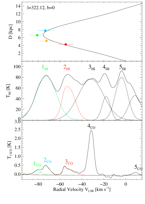
The bottom panel of Fig. 13 shows the CO spectrum integrated over the entire grid of rings identified in the XMM-Newton image in Fig. 8, smoothed with a $2\,{\rm km\,s^{-1}}$ FWHM Gaussian for noise removal. The spectrum shows five well identified, localized components of molecular gas in the direction of Circinus X-1. A simple multi-Gaussian fit (shown in color in the plot) locates the components at velocities $v_{\rm LOS,1}=-81\,{\rm km\,s^{-1}}$, $v_{\rm LOS,2}=-73\,{\rm km\,s^{-1}}$, $v_{\rm LOS,3}=-55\,{\rm km\,s^{-1}}$, $v_{\rm LOS,4}=-32\,{\rm km\,s^{-1}}$, and $v_{\rm LOS,5}=9\,{\rm km\,s^{-1}}$, where component 3_CO requires two Gaussian components to fit at $-50\,{\rm km\,s^{-1}}$ and $-55\,{\rm km\,s^{-1}}$.

Figure 14.— Differential (black) and total (gray) Mopra ¹²CO spectra of three ring sections (see Fig. 8 for a definition of the ring sections), smoothed with a $3\,{\rm km\,s^{-1}}$ FWHM Gaussian. Differential spectra show comparisons between neighboring ring sections that have large vs. small dust scattering intensity to isolate the CO velocity component responsible for the X-ray peak. Bottom: ring section [a11] minus [a12], middle: ring section [b6] minus [b7]; top: sum of ring sections [c5:8] minus sum of [c1:4].

While other components of cold gas are likely present below the sensitivity limit of the survey, and while some of the components may be superpositions of several distinct clouds it is clear from the spectrum that these are the primary concentrations of cold gas along the line-of-sight and therefore the most probable locations of the dust clouds responsible for the observed X-ray light echo.

We adopt the Galactic rotation curve by McClure-Griffiths & Dickey (2007) for the fourth Galactic quadrant within the Solar circle. We use the rotation curve by Brand & Blitz (1993) for the outer Galaxy, matched at $v_{\rm LSR}=0$ following the procedure used in Burton et al. (2013), for the Galactic position of Circinus X-1. The resulting radial velocity curve in the direction of Circinus X-1 as a function of distance from the Sun is plotted in the top panel of Fig. 13. Because the direction to Circinus X-1 crosses the Solar circle, the distance-velocity curve is double-valued, and we cannot simply associate a particular velocity with a given distance.

The rotation curve turns over at a minimum velocity of $v_{\rm rad}\geq-75.3\,{\rm km\,s^{-1}}$. Any velocity component at velocities beyond the minimum must be displaced from the Galactic rotation curve and lie near the tangent point. Given the velocity dispersion of molecular clouds of $\sigma_{\rm CO}\mathrel{\hbox{\hbox to0.0pt{\hbox{\lower 4.0pt\hbox{$\sim$}}\hss}\hbox{$<$}}}5\,{\rm km\,s^{-1}}$ relative to the LSR (see §4), velocities of $v_{\rm rad}\mathrel{\hbox{\hbox to0.0pt{\hbox{\lower 4.0pt\hbox{$\sim$}}\hss}\hbox{$>$}}}-80\,{\rm km\,s^{-1}}$, as measured for component 1_CO are consistent with the rotation curve and place the material at a distance of roughly $D\sim 6-8\,{\rm kpc}$.

Figure 15.— Adaptively smoothed Mopra ¹²CO image of component 2_CO in the velocity range $-76\,{\rm km\,s^{-1}}$ to $-72\,{\rm km\,s^{-1}}$. The image shows a clear lane of dense molecular gas across the image. Overlaid for comparison is the angular grid used to denote rings in Fig. 8. Connected blue dots are the local surface brightness peaks in ring [a11] from Chandra ObsID 15801, XMM ObsID 0729560501, and XMM ObsID 0729560601, showing a clear spatial coincidence with the CO lane. Also overlaid are the centroids (dots) and FWHMs (arcs) of the peaks in the angular intensity distributions of rings [a]-[d] from inside out in blue, green, yellow, and red, respectively, determined from spectral fits to Chandra ObsID 15801 in 10-degree segments for each ring. Note that the arc for ring [a] denotes the secondary peak. The peak of ring [c] is close to the chip edge, indicated by the arrow denoting the lower limit to the ring extent.

Given a rotation curve, one could attempt a global distance estimate by simply comparing ring radii and CO velocities. However, a considerably more robust and accurate distance estimate can be derived by also considering the angular distribution of dust inferred from the brightness of each of the rings as a function of azimuthal angle.

3.3.1 Differential CO spectra

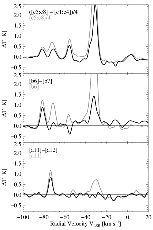
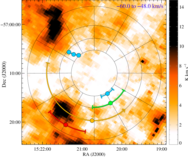
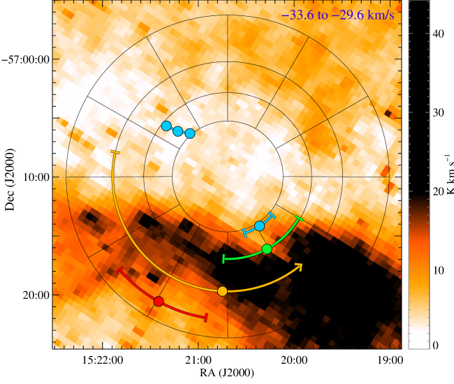
In order to identify which cloud is responsible for which ring, we generated adaptively smoothed images of each velocity component within velocity ranges centered on the CO velocity peaks of the clouds. The images are shown in Figs. 15-19 and discussed in §3.3.2. We also generated CO difference spectra to identify which velocity components may be responsible for the clear brightness enhancements seen in the different rings. They are plotted in Fig. 14, which we will discuss below.

The un-absorbed X-ray intensity shown in Figs. 6 and 8 is directly proportional to the scattering dust column density. Variations in $I_{2-5keV}$ as a function of azimuthal angle therefore probe the spatial distributions of the dust clouds responsible for the different rings. We can use a differential ¹²CO spectrum of two ring sections that have significantly different X-ray brightness to identify possible ¹²CO velocity components that show a marked difference in column density consistent with the dust enhancement.

Table 2Gaussian fits to CO velocity components for rings [a]-[d]

CO cloud	$v_{\rm CO}[{\rm km\,s^{-1}}]$	$\sigma[{\rm km\,s^{-1}}]$	$\frac{N_{\rm H_{2}}}{x_{\rm CO,20.3}}[10^{20}\,{\rm cm^{-2}}]$
Ring [a]:
Cloud 2CO	$-73.56\pm 0.12$	$1.46\pm 0.12$	$5.09\pm 0.97$
Ring [b]:
Cloud 1CO	$-80.85\pm 0.19$	$2.01\pm 0.20$	$3.88\pm 0.97$
Ring [c]:
Cloud 1CO	$-81.18\pm 0.15$	$1.72\pm 0.16$	$2.85\pm 0.35$
Cloud 2CO	$-72.44\pm 0.09$	$2.35\pm 0.09$	$7.71\pm 0.40$
Cloud 3CO	$-55.39\pm 0.08$	$1.82\pm 0.08$	$5.76\pm 0.34$
Cloud 4CO	$-31.16\pm 0.02$	$2.16\pm 0.02$	$36.02\pm 0.38$
Ring [d]:
Cloud 1CO	$-81.29\pm 0.16$	$1.93\pm 0.17$	$3.43\pm 0.76$
Cloud 2CO	$-72.14\pm 0.11$	$2.69\pm 0.12$	$7.59\pm 0.90$
Cloud 3CO	$-54.80\pm 0.09$	$2.26\pm 0.10$	$7.10\pm 0.78$
Cloud 4CO	$-30.85\pm 0.02$	$2.03\pm 0.02$	$34.22\pm 0.73$

Note. — ¹²CO spectra are integrated over rings of radii $4.0^{\prime}<R_{a}<6.0^{\prime}$, $6.0^{\prime}<R_{b}<8.5^{\prime}$, $8.5<R_{c}<12.0^{\prime}$, and $11.0^{\prime}<R_{d}<14.0^{\prime}$, respectively, weighted by the 3-5 keV Chandra intensity. Only velocity components identified in the differential CO spectra plotted in Fig. 14 as possible locations of dust responsible for the rings are listed

The two most obvious regions of strong local variation in $I_{2-5\,{\rm keV}}$ are seen at ring sections [a11] and [b6], both of which are significantly brighter than the neighboring sections [a12] and [b7], respectively.

In the bottom panel of Fig. 14, we show the difference ¹²CO spectrum of rings sections [a11] minus [a12] (i.e., the spectrum of [a12] subtracted from the spectrum of [a11]) as a thick black line. We also show the spectrum of [a11] only (i.e., without subtracting [a12]) as a thin gray line. Because of the strong enhancement in dust detected in [a11], the corresponding CO velocity component must be significantly brighter in [a11] as well, and therefore appear as a positive excess in the difference spectrum. It is clear from the figure that only one velocity component is significantly enhanced in [a11] relative to [a12], the one at $v_{\rm rad}=-74\,{\rm km\,s^{-1}}$. We can therefore unequivocally identify velocity component 2_CO at $-74\,{\rm km\,s^{-1}}$ as the one responsible for ring [a].

The middle panel of Fig. 14 shows the difference ¹²CO spectrum of [b6] minus [b7], where the light echo is significantly brighter in [b6] than [b7]. In this case, two ¹²CO velocity components are significantly enhanced in [b6] relatively to [b7], component 1_CO at $v_{\rm rad}\sim-80\,{\rm km\,s^{-1}}$ and component 4_CO at $v_{\rm rad}\sim-32\,{\rm km\,s^{-1}}$. While we cannot uniquely identify which velocity component is responsible for ring [b] from the spectra alone, we can rule out components 2_CO and 3_CO.

Finally, ring [c] does not show a single clearly X-ray enhanced section relative to neighboring ones. Instead, the Southern sections [c5:c8] are significantly enhanced relative to the Northern sections [c1:c4]. We therefore plot the difference CO spectrum of sections [c5] through [c8] minus sections [c1] through [c4] (top panel of Fig. 14). In this case, all four velocity components are enhanced in [c5:c8] relative to [c1:c4], and we cannot identify even a sub-set that is responsible for ring [c] from the difference spectrum alone.

Figure 16.— Adaptively smoothed Mopra ¹²CO image of component 1_CO in the velocity range $-85\,{\rm km\,s^{-1}}$ to $-75\,{\rm km\,s^{-1}}$, same nomenclature as in Fig. 15. The CO emission in this band shows a clear peak at locations [b5] and [b6], matching the intensity distribution of X-ray ring [b] (green ring segment).

3.3.2 CO images

In order to compare the ring emission with the spatial distribution of cold gas and dust in the different velocity components identified in Fig. 13, we extracted images around the peak of each velocity component, adaptively smoothed to remove noise in velocity channels of low-intensity while maintaining the full Mopra angular resolution in bright velocity channels. We employed a Gaussian spatial smoothing kernel with width $\sigma=1.5^{\prime}\times[1.0-0.9\exp[-(v-v_{\rm peak})/(2\sigma_{\rm CO}^{2})]$, where $v_{\rm peak}$ and $\sigma_{\rm CO}$ are the peak velocity and the dispersion of Gaussian fits to the summed CO spectra shown in Fig. 14. This prescription was chosen heuristically to produce sharp yet low-noise images of the different CO clouds.

The CO intensity maps can be compared with the locations of excess X-ray dust scattering to identify potential CO clouds responsible for the different rings, supporting the spectral identification of possible velocity components in §3.3.1 and Fig. 14. To quantify the deviation of the X-ray rings from axi-symmetry and for comparison with the CO data, we constructed azimuthal intensity profiles of the rings from Chandra ObsID 15801 in ten degree bins, following the same spectral fitting procedure used to construct Figs. 6 and 7. Ring radii in the ranges [a]: 4’-6’, [b]: 6’-8’, [c]: 9’-10’.5, [d]: 11’.5-12’.75 were chosen to best isolate each ring. The centroids and FWHM of the intensity peaks determined from Gaussian fits for each ring are plotted as colored circles and arcs in Figs. 15 -19, respectively.

Figure 17.— Adaptively smoothed Mopra ¹²CO image of component 2_CO,b in the velocity range $-72\,{\rm km\,s^{-1}}$ to $-67\,{\rm km\,s^{-1}}$, same nomenclature as in Fig. 15. The CO intensity peak matches the centroid of X-ray ring [c] (yellow arc).

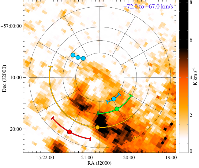
It is important to note that a one-to-one match in the intensity distribution should not be expected on large scales for every ring for three reasons: (a) multiple distinct clouds at different distances may fall into the same velocity channel because of velocity deviations of the clouds from the local standard of rest; (b) clouds at different distances may fall into the same velocity channel because of the double-valued nature of the distance-velocity curve; (c) individual rings may contain scattering contributions from multiple clouds at different velocities but similar distances.

However, clear local maxima in scattering intensity may be expected to correspond to local maxima in CO emission, and we will base possible cloud-ring identification on local correspondence. Indeed, detailed matches exist for rings [a] and [b], as already expected from the spectra discussed in §3.3.1, as well as for ring [d]:

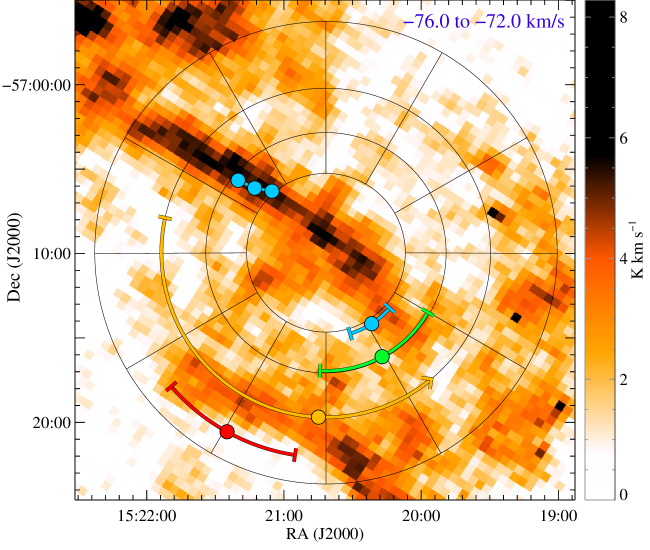
• Figure 15 shows an image of CO component 2_CO, integrated over the velocity range $-76\,{\rm km\,s^{-1}}<v_{\rm rad}<-72\,{\rm km\,s^{-1}}$, bracketing the velocity component at $v_{\rm rad}\sim-74\,{\rm km\,s^{-1}}$ identified in the differential spectra as giving rise to ring [a]. The clear association of ring [a] with component 2_CO at $-74\,{\rm km\,s^{-1}}$ in the CO image is striking. The prominent spectral feature at $v_{\rm rad}\sim-74\,{\rm km\,s^{-1}}$ corresponds to a well-defined lane that runs through the position of Circinus X-1 and crosses ring section [a11]. Overlaid as connected blue circles are the positions of the X-ray surface brightness peaks of ring [a] from Chandra ObsID 15801, and XMM ObsID 0729560501 and 0729560601 (from inside out, given the increasing ring radius at longer time delays for later observations). The intensity peak lies exactly on top of the CO peak and traces the CO lane as the rings sweep out larger radii.

  The obvious spatial coincidence and the fact that this is the only velocity component standing out in the differential spectrum of ring [a11] in Fig. 14 unambiguously determines that ring [a] must be produced by the dust associated with the CO cloud 2_CO at $v_{\rm rad}\sim-74\,{\rm km\,s^{-1}}$.

  In addition to the narrow lane in the North-Eastern quadrant of the image that we identify with the cloud responsible for ring [a], there is an additional concentration of CO emission in this channel in the Southern half of the image, which we identify as the cloud likely responsible for at least part of ring [c], and which we discuss further in Fig. 17.

  This velocity channel straddles the tangent point at minimum velocity $-75.3\,{\rm km\,s^{-1}}$ and may contain clouds of the distance range from 5kpc to 8 kpc (accounting for random motions). It is therefore plausible that multiple distinct clouds may contribute to this image and it is reasonable to associate features in this image with both rings [a] and [c].

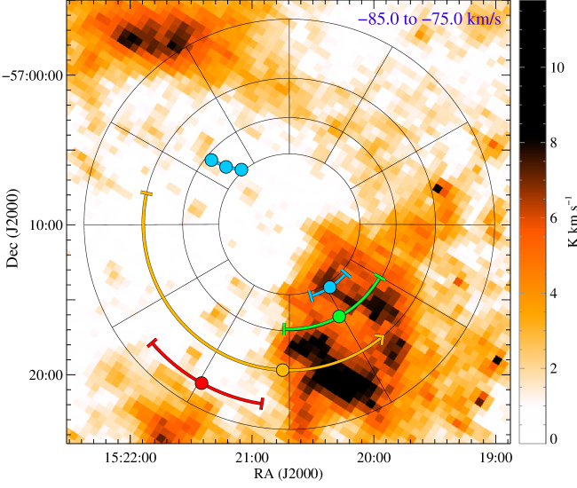
• Figure 16 shows the ¹²CO image of cloud 1_CO in the velocity range $-85\,{\rm km\,s^{-1}}<v_{\rm rad}<-75\,{\rm km\,s^{-1}}$, roughly centered on the peak at $-81\,{\rm km\,s^{-1}}$. The peak of the emission falls into sectors [b5:b6] and [c5:c6], while there is consistent excess CO emission in the Eastern part of ring [b]. This spatial coincidence with the observed excess scattering emission of ring [b] strongly suggests that cloud 1_CO is responsible for the bulk of the X-ray scattering for ring [b], consistent with the difference spectrum in the middle panel of Fig. 14. Because of the strong excess foreground absorption in these ring sections (see Fig. 9), a direct comparison with the intensity peaks in the X-ray images is more difficult than in the case of ring [a] (because the 3-5 keV channel images are significantly more noisy than the 1-2 keV and 2-3 keV channels, which are more strongly affected by absorption). However the clear X-ray intensity peak in sections [b5:b6] denoted by the green arc determined from the spectra correlates well with the peak in CO emission of cloud 1_CO.

• Figure 17 shows a low-band image of component 2_CO in the velocity range $-72\,{\rm km\,s^{-1}}<v_{\rm rad}<-67\,{\rm km\,s^{-1}}$. The CO emission peaks in sections [c5:c7] and corresponds to the centroid in the X-ray intensity of ring [c], which is overplotted as a yellow arc. The good spatial correspondence suggests that ring [c] is produced by a CO cloud at similar velocity but smaller relative distance than the CO cloud responsible for ring [a] shown in Fig. 15. Because of the substantial spectral overlap of both clouds, this image may not show the entire extent of the Southern part of component 2_CO.

• Figure 18 shows an image of cloud 3_CO in the velocity range $-60\,{\rm km\,s^{-1}}<v_{\rm rad}<-48\,{\rm km\,s^{-1}}$. The CO emission peaks in section [c8], coincident with the peak in the X-ray intensity of ring [d] at the same location (Fig. 8).

  Given the presence of several CO components in the Southern half of the image, identification of the intensity peaks of overlapping rings [c] and [d] is not as straight forward. However, it is clear that not all of rings [c] and [d] can be explained by component 3_CO alone. An additional contribution from material in other velocity channels is required to explain the excess emission in section [c5:c6]. Our discussion of Fig. 17 suggests that the Southern component of 1_CO is the second component responsible for rings [c] and/or [d].

• Figure 19 shows an image of cloud 4_CO in the velocity range $-33.6\,{\rm km\,s^{-1}}<v_{\rm rad}<-29.6\,{\rm km\,s^{-1}}$, which is the dominant CO component in the Mopra FOV. A very bright lane of molecular gas is crossing the Southern half of the FOV through sections [c5], [b5:b7]. Comparison with the X-ray images shows a clear spatial overlap of this CO cloud with the bluest sections of the ring emission that we identified as foreground absorption above. A contour of this cloud is overlaid on Figs. 5 and 7 and traces the region of highest column density very closely.

  Because component 4_CO causes absorption in rings [b], [c], and [d] without a correspondingly large scattering intensity peak (which would have to be about an order of magnitude brighter than the other rings, given the very large column density of component 4_CO), the main component of cloud 4_CO must be in the foreground relative to the clouds generating the scattering emission of X-ray rings [b], [c], and [d]. The brightest parts of this cloud are almost certainly optically thick in ¹²CO. The estimate of the cloud column density for this feature based on the ¹²CO intensity in Table 2 is therefore likely an underestimate. In fact, the differential hydrogen column inferred from the X-ray spectra, roughly $N_{\rm H}\sim 10^{22}\,{\rm cm^{-2}}$, is about a factor of two to three larger than that inferred from ¹²CO.

Figure 18.— Adaptively smoothed Mopra ¹²CO image of component 3_CO in the velocity range $-60\,{\rm km\,s^{-1}}$ to $-48\,{\rm km\,s^{-1}}$, same nomenclature as in Fig. 15. The CO intensity peak in the Southern half matches the location of the intensity peak of ring [d] (limited to the Chandra FOV; red arc).

From the image comparisons and the differential CO spectra, a clear picture regarding the possible ring-cloud association emerges: Ring [a] must be generated by cloud 2_CO at $\sim-74\,{\rm km\,s^{-1}}$. Ring [b] is generated by cloud 1_CO at $\sim-81\,{\rm km\,s^{-1}}$. At least part of the emission of ring [c] or [d] is likely generated by cloud 3_CO, but an additional component is required to explain the emission in [c5:c6].

4. Discussion

4.1. The distance to Circinus X-1 

Based on the ring-cloud association discussed in the previous section, we can use the kinematic distance estimate to each cloud from the ¹²CO velocity and the relative distance $x$ to the cloud from the light echo to constrain the distance to Circinus X-1.

To derive kinematic distances to the clouds, we assume that the molecular clouds measured in our CO spectra generally follow Galactic rotation, with some random dispersion around the local standard of rest (LSR). Literature estimates for the value of the 1D velocity dispersion $\sigma_{\rm cloud}$ range from $\sigma_{\rm cloud}\sim 3.5\,{\rm km\,s^{-1}}$ (Liszt & Burton, 1981) for GMCs in the inner Galaxy to $7\,{\rm km\,s^{-1}}$ (Stark, 1984; Stark & Brand, 1989) for moderate-mass high latitude clouds in the Solar Galactic neighborhood. Recent studies of kinematic distances to clouds assume a 1D dispersion of $\sigma_{\rm cloud}\sim 3\,{\rm km\,s^{-1}}$ around the LSR (e.g. Roman-Duval et al., 2009; Foster et al., 2012). In the following, we will conservatively adopt a value of $\sigma_{\rm cloud}\sim 5\,{\rm km\,s^{-1}}$.

Figure 19.— Adaptively smoothed Mopra ¹²CO image of component 4_CO in the velocity range $-33.6\,{\rm km\,s^{-1}}$ to $-29.6\,{\rm km\,s^{-1}}$, showing the brightest emission feature in the field of view; same nomenclature as in Fig. 15. The band of molecular gas across the lower half of the image matches the band of absorption seen in the color images in Fig. 4 and 5 in position and morphology and corresponds to the excess absorption found in the spectrally determined absorption column shown in Figs. 7 and 9.

In addition to random cloud motions, an unknown contribution from streaming motions may be present. The magnitude of streaming motions relative to estimates of the Galactic rotation curve is generally relatively poorly constrained observationally (Roman-Duval et al., 2009; Reid et al., 2014). McClure-Griffiths & Dickey (2007) characterized the possible contribution of streaming motions to deviations from the rotation curve in the fourth quadrant and found systematic deviations due to streaming motions with a peak-to-peak amplitude of $10\,{\rm km\,s^{-1}}$ and a standard deviation of $\sigma_{\rm streaming}\sim 5\,{\rm km\,s^{-1}}$. While streaming motions are not completely random, the four dust clouds responsible for the rings are located at sufficiently different distances that their streaming motions relative to the Galactic rotation curve may be considered as un-correlated. Thus, we will treat the uncertainty associated with streaming motions as statistical and add the dispersion $\sigma_{\rm streaming}$ in quadrature to the cloud-to-cloud velocity dispersion, giving an effective 1D bulk velocity dispersion relative to Galactic rotation of $\sigma_{\rm cloud,eff}\sim 7\,{\rm km\,s^{-1}}$.

We assume that the main component of each dust cloud identified in Fig. 12 and Table 1 is associated with one of the CO velocity components identified above. However, a single velocity component may be associated with more than one ring, given the double-valued nature of the velocity curve and the possible overlap of clouds in velocity space due to excursions from the LSR. For a given a distance $D$ to Circinus X-1, we can then determine the radial velocity of each dust cloud if it were at the LSR, given its relative distance $x(D,\theta_{\rm med})$, and compare it to the observed radial velocities of the CO clouds.

For an accurate comparison, we extracted CO spectra that cover the FOV of Chandra ObsIDs 15801 and 16578, limited to the radial ranges [a]: 4.0’-6.0’, [b]: 6.0’-8.5’, [c]: 8.5’-12’, [d]: 11.0’-14.0’ for ObsId 15801 and increase radial ranges by 4% for ObsID 16578 according to eq. (10). We weighted the CO emission across the FOV with the 3-5 keV Chandra intensity in order to capture CO emission from the regions of brightest dust scattering. We fitted each identified CO component with a Gaussian and list the relevant CO clouds used in the fits in Table 2.

For a given assumed distance $D$ to Circinus X-1, we calculate the expected radial velocities of the cloud components and compare them to the observed CO velocities to find the distance that best matches the observed distribution of clouds. We represent each CO cloud $j$ and each dust cloud $i$ by the best-fit Gaussians from Tables 2 and 1, respectively, with dispersions $\sigma_{\rm CO,j}$ and $\sigma_{\rm dust,i}$ and peak positions $v_{\rm CO,j}$ and $v_{\rm dust,i}$, respectively. In addition, we allow for an effective bulk 1D velocity dispersion of $\sigma_{\rm cloud,eff}=7\,{\rm km\,s^{-1}}$ relative to the Galactic rotation curve as discussed above, comprised of the random cloud-to-cloud velocity dispersion and contributions from streaming motions.

Figure 20.— Unnormalized posterior of the distance to Circinus X-1 from ObsID 15801 and 16578. Shown in black: Likelihood function with all three priors about ring-CO-cloud associations in place (i.e., we identify velocity component 2_CO at $v_{\rm LOS}\approx-74\,{\rm km\,s^{-1}}$ with ring [a], component 1_CO at $v_{\rm LOS}\approx-80\,{\rm km\,s^{-1}}$ with the peak of ring [b], and require ring [c] and [d] to be produced by different CO components). The likelihood distributions without any priors, with only prior one, and with prior one and two are plotted as dotted, dashed, and solid gray curves, respectively. The most likely distance of $9.4\,{\rm kpc}$ and the 1-sigma and 3-sigma uncertainties are plotted as solid, dashed, and dashed-triple-dotted gray vertical lines, respectively.

While the velocity distribution of each dust cloud (calculated from the Gaussian fit to the distribution of dust as a function of $z$) is not itself Gaussian, we conservatively use the peak value of the velocity and assign a velocity dispersion $\sigma_{\rm dist,i}$ that is the larger of the two propagated $z$-dispersions in the positive and negative $z$-direction from the peak of the cloud.

We combine the measurements on the ring radii from the deconvolutions of ObsID 15801 and 16578, corrected by the expansion factor of the rings given by eq. (10). The goodness of fit is then determined by the likelihood function $P(D)$ as a function of distance $D$,

$$P(D)=\frac{1}{N_{P}}\times...$$

$$...\,{\Pi_{i=1}^{4}\,{\rm max}_{j_{i}=1}^{4}\left\{\exp{\left[-\frac{\left(v_{\rm dust,i}(D)-v_{\rm CO,j_{i}}\right)^{2}}{2\left(\sigma_{\rm dust,i}^{2}+\sigma_{\rm CO,j_{i}}^{2}+\sigma_{\rm cloud}^{2}\right)}\right]}\right\}}$$

where for each dust cloud $i$ in the product, the CO component $j_{i}$ with the maximum likelihood is chosen from the set of allowed CO components, i.e., the CO component that most closely matches the velocity $v_{\rm dist,i}$ of dust cloud $i$; $N_{P}$ is a normalization factor chosen to ensure that $\int dDP(D)=1$. $P(D)$ is plotted in Fig. 20.

As discussed in §3.3.2, we can restrict the CO clouds responsible for the rings based on the visual and spectral identification discussed in §3.3.1 and §3.3.2. We place two strong priors and one weak prior on the association of dust and CO clouds:

1. The first strong prior is the association of ring [a] with CO component 2_CO

2. The second strong prior is the association of ring [b] with CO component 1_CO

3. The third, weak prior is the requirement that ring [c] and [d] cannot be produced by component 3_CO alone, i.e., that either ring [c], or ring [d] are associated with a component other than 3_CO.

Functionally, these priors take the form of limits on the possible combinations of rings $i$ and clouds $j_{i}$ in the maximum taken in eq. (4.1). That is, the first prior eliminates the maximum for ring $i=1$ and simply replaces it with the exponential for cloud $j_{1}=2$, while the second prior replaces the maximum for ring $i=2$ with the exponential for $j_{2}=1$. The third prior eliminates combinations in the maximum for which $j=3$ for both $i=3$ and $i=4$.

4.1.1 Distance estimate with all three priors

With all three priors in place, eq. (4.1) takes the form

$$P(D)=\frac{1}{N_{P}}\times...$$

$$...\exp{\left[{-\frac{\left(v_{\rm dust,1}(D)-v_{\rm CO,2}\right)^{2}}{2\left(\sigma_{\rm dust,1}^{2}+\sigma_{\rm CO,2}^{2}+\sigma_{\rm cloud,eff}^{2}\right)}}\right]}\times...$$

$$...\exp{\left[{-\frac{\left(v_{\rm dust,2}(D)-v_{\rm CO,1}\right)^{2}}{2\left(\sigma_{\rm dust,2}^{2}+\sigma_{\rm CO,1}^{2}+\sigma_{\rm cloud,eff}^{2}\right)}}\right]}\times...$$

$$...\Pi_{i=3}^{4}\,{\rm max}_{j_{i}=1}^{4}\left\{\left(1-\delta_{j_{3},3}\delta_{j_{4},3}\right)\times...\vphantom{\exp{\left[-\frac{\left(v_{\rm dust,i}(D)-v_{\rm CO,j_{i}}\right)^{2}}{2\left(\sigma_{\rm dust,i}^{2}+\sigma_{\rm CO,j_{i}}^{2}+\sigma_{\rm cloud,eff}^{2}\right)}\right]}}\right.$$

$$\ \ \ \ \ \ \ \ \ \ \ \ \ \ \ \left....\exp{\left[-\frac{\left(v_{\rm dust,i}(D)-v_{\rm CO,j_{i}}\right)^{2}}{2\left(\sigma_{\rm dust,i}^{2}+\sigma_{\rm CO,j_{i}}^{2}+\sigma_{\rm cloud,eff}^{2}\right)}\right]}\right\}$$

where the product $\delta_{j_{3},3}\delta_{j_{4},3}$ of two Kronecker deltas guarantees that rings [c] and [d] cannot both be produced by CO cloud $j=3$, since the term in parentheses vanishes when $j_{3}=j_{4}=3$.

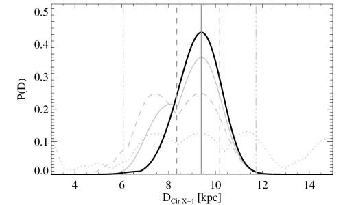
The likelihood distribution with all three priors in place is shown as a solid black curve in Fig. 20. The 68% and 99.7% confidence intervals (corresponding to the one- and three-sigma uncertainties in the distance to Circinus X-1) are plotted as well.

The best fit distance to Circinus X-1 with 1-sigma statistical uncertainties is

$$D_{\rm CirX-1}=9.4^{+0.8}_{-1.0}\,{\rm kpc}$$ (13)

Quantities that depend on $D_{\rm CirX-1}$ listed in this paper (such as the relative cloud distance $x$) are calculated using the best fit value from eq. (13) and are listed in gray color in Table 1 and Fig. 12.

The distance listed in eq. (13) is consistent with the dust-cloud associations of rings [a] and [b] with clouds 2_CO and 1_CO, respectively, it places the cloud responsible for rings [c] and [d] at velocities associated with CO components 2_CO and 3_CO, respectively, and it places the CO mass of cloud 4_CO in the foreground of all of the scattering screens, consistent with the observed excess photo-electric absorption observed in the X-ray images that coincides with the location of cloud 4_CO. The locations and velocities to the four scattering screens derived from the best fit distance are plotted in the top panel of Fig. 13, showing that the dust clouds fall close to the Galactic rotation curve.

We overplot the best-fit distance and velocity scale as a function of observed angle $\theta$ in gray on the top x-axis in Fig. 12. Figure 12 also shows the scattering depth $\left.N_{\rm H}d\sigma/d\Omega\right|_{\rm med}$ in gray. Because it requires knowledge of $x(D)$, this quantity is distance dependent.

The distance derived here is both geometric and kinematic, given that we use kinematic distances to molecular clouds to anchor the absolute distance scale, and more accurate relative geometric distances to the scattering screens. As such, one might refer to this method as either pseudo-kinematic or pseudo-geometric. Given that the predominant error in our method stems from the kinematic aspect of the distance determination, we will simply refer to it as a kinematic distance.

For completeness, we will also list the constraints on the distance with only a sub-set of priors 1-3 in place:

4.1.2 Distance estimate with the two strong priors only

With both prior 1 and 2 in place, a secondary peak appears at $7.8\,{\rm kpc}$ (solid gray curve in Fig. 20), with a three-sigma lower limit of $D_{\rm Cir}>6.3\,{\rm kpc}$. This peak corresponds to the solutions for which both ring [c] and [d] are produced by cloud 3_CO. The formal one-sigma uncertainty of the distance to Circinus X-1 from only the two strong priors 1 and 2 is $D_{\rm CirX-1}=9.4^{+0.8}_{-1.7}\,{\rm kpc}$.

4.1.3 Distance estimate with only prior 1 in place

With only the first prior in place, the likelihood distribution has two roughly equally strong peaks, one at $7.4\,{\rm kpc}$ and one at $9.4\,{\rm kpc}$ (dashed gray curve in Fig. 20), and the possible distance range is restricted from 4.5 to 11 kpc. The second strong peak at lower distance corresponds to a solution for which both rings [a] and [b] are associated with component 1_CO and rings [c] and [d] are associated with component 3_CO.

4.1.4 Lack of distance constraints without any priors

Without placing any priors on dust-CO cloud associations, the source distance is not formally constrained, as can be seen from the dotted curve in Fig. 20, which has multiple peaks at distances from 3 to 15 kpc.

4.2. Implications of a Distance of $9.4\,{\rm kpc}$ for the Properties of Circinus X-1 

Our three-sigma lower limit of $D>6.1\,{\rm kpc}$ on the distance to Circinus X-1 is inconsistent with previous claims of distances around 4 kpc (Iaria et al., 2005). On the other hand, the 1-sigma distance range listed in eq. (13) is consistent with the distance range of $7.8-10.5\,{\rm kpc}$ based on the observations of type I X-ray bursts by Jonker & Nelemans (2004), which further strengthens the case for the kinematic distance presented here.

A distance of $9.4\,{\rm kpc}$ is only marginally larger than the fiducial value of $8\,{\rm kpc}$ adopted in Heinz et al. (2013). The age of the supernova remnant and thus the age of the X-ray binary increases slightly to $t_{\rm Cir}\sim 3,000\,{\rm yrs}$, well within the uncertainties estimated in Heinz et al. (2013), while the supernova energy would increase by about 40%.

At a distance of 9.4 kpc, the X-ray binary itself has exceeded the Eddington luminosity for a 1.4 solar mass neutron star frequently during the time it has been monitored by both the All Sky Monitor on the Rossi X-ray Timing Explorer and MAXI, most recently during the 2013 flare that gave rise to the rings reported here. For example, during the peak of its bright, persistent outburst between about 1995 and 1997, the mean 2-10 keV luminosity of the source was approximately $L_{\rm 1995,2-10keV}\sim 3\times 10^{38}\,{\rm ergs\,s^{-1}}\,\left(D/9.4\,{\rm kpc}\right)^{-2}$. We estimate the peak flux measured by MAXI during the 2013 flare to be about 2.2 Crabs, corresponding to a peak luminosity of $L_{\rm peak,2-10keV}\sim 5.6\times 10^{38}\,{\rm ergs\,s^{-1}}\,\left(D/9.4\,{\rm kpc}\right)^{-2}$.

One of the most intriguing properties of Circinus X-1 is the presence of a powerful jet seen both in radio (Stewart et al., 1993) and X-rays (Heinz et al., 2007). Fender et al. (2004a) reported the detection of a superluminal jet ejection, launched during an X-ray flare. Taken at face value, the observed proper motion of $\mu\sim 400\,{\rm mas\,day^{-1}}$ at a distance of $9.4\,{\rm kpc}$ implies an apparent signal speed and jet Lorentz factor of $\Gamma\mathrel{\hbox{\hbox to0.0pt{\hbox{\lower 4.0pt\hbox{$\sim$}}\hss}\hbox{$>$}}}\beta_{\rm app}=v_{\rm app}/c\mathrel{\hbox{\hbox to0.0pt{\hbox{\lower 4.0pt\hbox{$\sim$}}\hss}\hbox{$>$}}}22\,\left(D/9.4\,{\rm kpc}\right)$ and a jet inclination of $\theta_{\rm jet}\mathrel{\hbox{\hbox to0.0pt{\hbox{\lower 4.0pt\hbox{$\sim$}}\hss}\hbox{$<$}}}3^{\circ}\left(9.4\,{\rm kpc}/D\right)$. This would make the jet in Circinus X-1 even more extreme than the parameters presented in Fender et al. (2004a), who assumed a fiducial distance of $6.5\,{\rm kpc}$.

4.3. The Galactic Positions of Circinus X-1 and Scattering Screens [a]-[d]

At a distance of around 9.4 kpc, Circinus X-1 is likely located inside the far-side of the Scutum-Centaurus arm. A location inside a (star forming) spiral arm is consistent with the young age of the binary.

The CO cloud nearest to the Sun, component 4_CO at $\sim-33\,{\rm km\,s^{-1}}$, is likely located in the near-side of the Scutum-Centaurus arm, explaining the large column density responsible for the foreground absorption.

CO clouds 1_CO through 3_CO are at intermediate distances; association of these clouds with either the Norma arm (or the Scutum-Centaurus arm for cloud 3_CO) are plausible but difficult to substantiate.

Section 4.1 discussed a possible error due to streaming motions of CO clouds relative to the LSR as part of the large scale Galactic structure. For streaming motions to strongly affect the measured radial velocity to a particular cloud, the cloud would have to be located near a major spiral arm.

The dominant spiral arm towards Circinus X-1 is the near side of the Scutum-Centaurus arm, which crosses the line-of-sight at roughly $3-4\,{\rm kpc}$, which we tentatively identified with cloud 4_CO. CO clouds 1_CO and 2_CO, which dominate the likelihood distribution plotted Fig. 20, are likely located far away from the center of that spiral arm. Thus, streaming motions are expected to be moderate (see, e.g., Jones & Dickey 2012 and the artist’s impression of Galactic structure by Benjamin & Hurt), which will limit the deviation of the observed radial velocity of cloud from Galactic rotation. Our error treatment is therefore conservative in including the full velocity dispersion of streaming motions as estimated by McClure-Griffiths & Dickey (2007) for the fourth quadrant.

Given the Galactic rotation curve plotted in Fig. 13, the radial velocity corresponding to a distance of 9.4 kpc at the Galactic position of Circinus X-1 is $v_{\rm LSR}=-54\,{\rm km\,s^{-1}}$. Jonker et al. (2007) found a systemic radial velocity of $v_{\rm rad,Cir}\sim-26\pm 3\,{\rm km\,s^{-1}}$, which would imply a 1D kick velocity of order $v_{\rm kick,LOS}\sim 25-35\,{\rm km\,s^{-1}}$, consistent with the values inferred for high-mass X-ray binaries in the SMC (Coe, 2005) and theoretical expectations for post-supernova center-of-mass velocities of high-mass X-ray binaries (Brandt & Podsiadlowski, 1995).

The potential association of Circinus X-1 with the CO velocity component 5_CO at $v_{\rm LOS}\approx 9\,{\rm km\,s^{-1}}$ suggested by Hawkes et al. (2014) would place Circinus X-1 at the very far end of the allowed distance range and require a very large relative velocity of that cloud with respect to the LSR at more than 30$\,{\rm km\,s^{-1}}$, both of which would correspond to three-sigma deviations. We therefore conclude that Circinus X-1 and cloud 5_CO are unassociated.

4.4. Constraints on the Dust Scattering Cross Section

The most robust constraints on the scattering cross section, and thus the properties of the dust responsible for the echo, would be derived by measuring the angular dependence of the brightness of a single ring over time. This is because such a measurement removes the large uncertainty in the total hydrogen column towards a particular cloud, since it would measure the relative change in brightness. Unfortunately, because our observations lack the temporal coverage to follow the brightness of each ring over a large range in scattering angle, as done by Tiengo et al. (2010), we cannot probe models of the dust scattering cross section at the same level of detail.

However, we can still place quantitative constraints on $d\sigma/d\Omega$, given the scattering depth of the rings shown in Table 1 and estimates of the hydrogen column density in both H₂ from CO and in neutral hydrogen from the 21cm data, we can derive constraints on the dust scattering cross section. The scattering angle and the scattering depth depend on $x(\theta,D)$, and the ring-cloud associations depend on distance as well.

Table 3Hydrogen column density for rings [a]-[d] from ¹²CO and 21cm spectra for Chandra ObsID 15801

Ring:	$N_{H_{2}}{\rm[10^{20}cm^{-2}]}$	$N_{HI}{\rm[10^{20}cm^{-2}]}$	$N_{H_{\rm tot}}{\rm[10^{20}cm^{-2}]}$
[a]	$5.1^{+5.1}_{-2.6}$	$17.1^{+17.6}_{-9.4}$	$27.3^{+20.3}_{-10.7}$
[b]	$3.9^{+3.9}_{-2.0}$	$13.4^{+13.7}_{-7.2}$	$21.2^{+15.7}_{-8.2}$
[c]	$7.7^{+7.7}_{-3.9}$	$32.4^{+32.9}_{-17.1}$	$47.9^{+36.3}_{-18.8}$
[d]	$7.1^{+7.1}_{-3.6}$	$20.6^{+20.6}_{-10.3}$	$34.8^{+25.0}_{-12.5}$

To derive an estimate of the molecular hydrogen column density, we used the values of N${}_{\rm H_{2}}$ from Table 3, adopting a value of the CO-to-H₂ conversion factor of $x_{\rm CO}=2\times 10^{20}$ (Bolatto et al., 2013), allowing for an extra factor of 2 uncertainty in $x_{\rm CO}$. It should be noted that $x_{\rm CO}$ may vary by up to an order of magnitude within individual clouds (Lee et al., 2014).

We estimated the neutral hydrogen column density from the 21cm Southern Galactic Plan Survey, following the same extraction regions used to derive the integrated CO intensity: We restricted the extraction region to the Chandra field of view and weighted the 21cm emission by the Chandra 3-5 keV surface brightness. We then fitted Gaussian lines to the velocity components, fixing the velocity centroids of the components to the CO velocities listed in Table 2.

Because the 21cm components are much broader than the CO components, clouds 1_CO and 2_CO are blended in 21cm emission and we cannot fit them as separate components. To estimate the HI column density in each component, we divide the total column in component 1_HI into two components with a column density ratio given by the ratio of the flux of the CO components 1_CO and 2_CO. We budgeted an additional factor of 2 uncertainty in the neutral hydrogen column derived from the 21cm data. The results are listed in Table 3.

Figure 21.— Dust scattering cross section as a function of scattering angle, determined from scattering depth (Table 1) and the column density from the measured ¹²CO intensity and 21cm HI intensity (Table 3), plotted for Chandra ObsID 15801 (circles), ObsID 16578 (squares) and XMM ObsID 0729560501 (triangles) for clouds [a],[b],[c], and [d] in green, blue, yellow, and red, respectively, evaluated at energy $E=2keV$. Overplotted is the predicted differential cross section from Draine (2003, solid black line) and the best fit powerlaw (dotted line). We do not include ring [d] for XMM ObsID 0729560501 because its centroid falls outside of the MOS FOV.

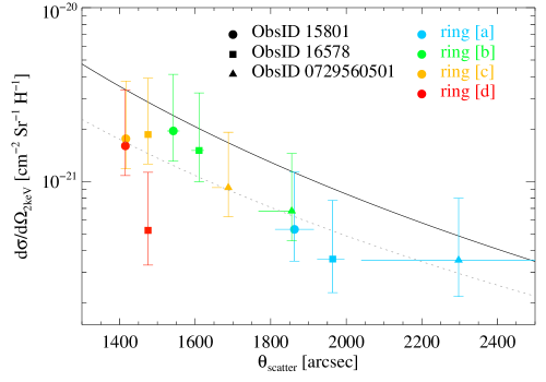
Figure 21 shows the differential X-ray scattering cross section $d\sigma/d\Omega_{\rm sc}$ per hydrogen atom as a function of scattering angle $\theta_{\rm sc}$, evaluated at 2 keV. Despite the relatively large scatter, the figure shows the expected decline with $\theta_{\rm sc}$. For comparison, the figure shows the scattering cross section derived by Draine (2003), which agrees relatively well with the observations in slope and normalization. Because we associated the entire amount of neutral hydrogen column in the velocity range $-85$ to $-30\,{\rm km\,s^{-1}}$ to the the four clouds, the derived cross sections may be regarded as lower limits, which may be responsible for the vertical offset between model and data.

We also plot the best-fit powerlaw fit to the cross section as a function of $\theta_{\rm sc}$ (dotted line):

$$\left.\frac{d\sigma}{d\Omega}\right|_{\rm 2\,{\rm keV}}\approx\left(5.8\pm 2.2\right)\times 10^{-21}\left(\frac{\theta_{\rm sc}}{1,000^{\prime}}\right)^{-3.6\pm 0.7}$$ (14)

It is clear that the large uncertainties in the total hydrogen column dominate the scatter and uncertainty in this plot. Higher resolution 21cm data woud likely improve the accuracy of this plot significantly. Ultimately, a direct correlation of the scattering depth with the absorption optical depth, neither of which depend on the column density of hydrogen, would provide a much cleaner measurement of the scattering cross section. Such an analysis is beyond the scope of this work, however.

4.5. Predictions for Future Light Echoes and the Prospects for X-ray Tomography of the ISM Towards Circinus X-1

The suitable long-term lightcurve and the location in the Galactic plane with available high-resolution CO data from the Mopra Southern Galactic Plane Survey make Circinus X-1 an ideal tool to study the properties of dust and its association with molecular gas.

Given our preferred distance to Circinus X-1, we can make clear predictions for observations of future light echoes. Since the four major rings described in this paper were produced by the molecular clouds associated with the CO velocity components 1_CO, 2_CO, and 3_CO, future X-ray observations of Circinus X-1 light echoes will show similar sets of rings, with radii for a given time delay determined from eq. (2) and Table 1.

The light echo produced by the CO cloud with the largest column density (cloud 4_CO) was already outside of the Chandra and XMM FOVs at the time of the observations. In order to confirm the dust-to-CO-cloud association presented in this paper, future X-ray observations of light echoes should include Chandra or Swift observations sufficiently close in time to the X-ray flare to observe the very bright light echo expected from cloud 4_CO, which we will refer to as the putative ring [e]. Ring [e] will be brightest in the Southern half of the image. Because Circinus X-1 exhibits sporadic flares several times per year, it should be possible to observe this echo with modest exposure times and/or for moderate X-ray fluence of the flare, given the expected large intensity of the echo due to the large column density of cloud 4_CO.

A detection of ring [e] would improve the fidelity of the distance estimate primarily because it would test the ring-cloud-associations assumed in our three priors. However, the statistical improvement on the distance estimate would be marginal because the low relative distance $x_{4_{\rm CO}}\sim 0.25$ to cloud 4_CO implies a large change in $x_{4_{\rm CO}}$ with $D$ in such a way that $D_{4_{\rm CO}}=x_{4_{\rm CO}}D$ (and thus also the velocity constraint on cloud 4_CO) is rather insensitive to $D$.

Future observations at smaller delay times will also provide constraints on the scattering cross section at smaller scattering angles. Constraints on $d\sigma/d\Omega$ from single rings at different scattering angles are inherently less error-prone, as the error in the normalization of $N_{\rm H}$ affects all measurement equally, probing the relative change of scattering cross section with $\theta_{\rm sc}$.

Better temporal coverage of the light echo from earlier times will allow detailed maps of each cloud both from the spatial distribution of the scattering signal and from the foreground absorption caused by each of the dust clouds, which can be compared to the scattering depth and the hydrogen column density from CO and HI measurements.

Should a high-accuracy distance determination to Circinus X-1 become possible from other methods, (such as maser parallax to one of the CO clouds, in particular cloud 4_CO, which has the highest column density, or VLBI parallax to the source itself), the distance to all dust components will be determined to within 5% accuracy or better (set by the relative angular width $\sigma_{\rm theta}/\theta_{\rm med}$ of the dust cloud from Table 1). This would allow for extremely accurate tomography of the dust and gas distribution towards Circinus X-1 from the existing observations presented here and any future light echo observations, providing a powerful tool to study Galactic structure in the fourth quadrant.

5. Conclusions

The giant flare and the associated X-ray light echo presented in this paper are the brightest and largest set of light-echo rings observed from an X-ray binary to date. The deviation from spherical symmetry allows us to make an unambiguous determination of the clouds responsible for part of the light echo from an X-ray binary.

Because of the full temporal coverage of the lightcurve of the X-ray flare by MAXI, we are able to reconstruct the dust distribution towards Circinus X-1 by deconvolving the radial profile with the dust scattering kernel derived from the X-ray lightcurve.

The kinematic distance of about 9.4 kpc we derived from the association of ring [a] with cloud 2_CO and ring [b] with cloud 1_CO is consistent with the estimate by Jonker & Nelemans (2004) based on the luminosity of the type I X-ray bursts of the source (Tennant et al., 1986). It places a large cloud of molecular gas (cloud 4_CO and the associated large absorption column in the Southern quadrant of the FOV) in the foreground of the dust screens detected in the light echo.

At a distance of about $9.4\,{\rm kpc}$, the source has exceeded the Eddington limit for a 1.4 $M_{\odot}$ neutron star frequently during the time it has been monitored by the All Sky Monitors on the Rossi X-ray Timing Explorer and MAXI, both during recent outbursts and, more importantly, in average luminosity during its persistent high-state in the 1990s.

Taken at face value, the observed pattern speeds in the jet (Fender et al., 2004b) indicate a very fast jet speed of $\Gamma\mathrel{\hbox{\hbox to0.0pt{\hbox{\lower 4.0pt\hbox{$\sim$}}\hss}\hbox{$>$}}}22$ and a correspondingly small viewing angle of $\theta_{\rm jet}\mathrel{\hbox{\hbox to0.0pt{\hbox{\lower 4.0pt\hbox{$\sim$}}\hss}\hbox{$<$}}}2.6^{\circ}$.

Future measurements of light echoes from Circinus X-1 will allow accurate measurements of the dust scattering cross section as a function of scattering angle and an estimation of the dust-to-gas ratio in the different clouds identified in the field of view towards Circinus X-1.

The technique used to derive the kinematic distance to Circinus X-1 holds significant promise for future observations of light echoes from X-ray transients.

References

- Asai et al. (2014) Asai, K., Mihara, T., Matsuoka, M., Sugizaki, M., Nakahira, S., Negoro, H., Nakajima, M., & Okazaki, A. T. 2014, PASJ, 66, 79
- Bolatto et al. (2013) Bolatto, A. D., Wolfire, M., & Leroy, A. K. 2013, ARA&A, 51, 207
- Brand & Blitz (1993) Brand, J. & Blitz, L. 1993, A&A, 275, 67
- Brandt & Podsiadlowski (1995) Brandt, N. & Podsiadlowski, P. 1995, MNRAS, 274, 461
- Brandt & Schulz (2000) Brandt, W. N. & Schulz, N. S. 2000, ApJ, 544, L123
- Burton et al. (2013) Burton, M. G., Braiding, C., Glueck, C., Goldsmith, P., Hawkes, J., Hollenbach, D. J., Kulesa, C., Martin, C. L., Pineda, J. L., Rowell, G., Simon, R., Stark, A. A., Stutzki, J., Tothill, N. J. H., Urquhart, J. S., Walker, C., Walsh, A. J., & Wolfire, M. 2013, PASA, 30, 44
- Calvelo et al. (2012) Calvelo, D. E., Fender, R. P., Tzioumis, A. K., Kawai, N., Broderick, J. W., & Bell, M. E. 2012, MNRAS, 419, 436
- Clarkson et al. (2004) Clarkson, W. I., Charles, P. A., & Onyett, N. 2004, MNRAS, 348, 458
- Coe (2005) Coe, M. J. 2005, MNRAS, 358, 1379
- Corrales & Paerels (2013) Corrales, L. & Paerels, F. 2013, ArXiv e-prints
- Draine (2003) Draine, B. T. 2003, ApJ, 598, 1026
- Fender et al. (2004a) Fender, R., Wu, K., Johnston, H., Tzioumis, T., Jonker, P., Spencer, R., & van der Klis, M. 2004a, Nature, 427, 222
- Fender et al. (2004b) Fender, R. P., Belloni, T. M., & Gallo, E. 2004b, MNRAS, 355, 1105
- Foster et al. (2012) Foster, J. B., Stead, J. J., Benjamin, R. A., Hoare, M. G., & Jackson, J. M. 2012, ApJ, 751, 157
- Freeman et al. (2002) Freeman, P. E., Kashyap, V., Rosner, R., & Lamb, D. Q. 2002, ApJS, 138, 185
- Hawkes et al. (2014) Hawkes, J., Rowell, G., Dawson, B., Aharonian, F., Burton, M., Fukui, Y., Furukawa, N., Hayakawa, T., Kawamura, A., Maxted, N., de Oña-Wilhelmi, E., de Wilt, P., & Walsh, A. 2014, International Journal of Modern Physics Conference Series, 28, 60198
- Heinz et al. (2007) Heinz, S., Schulz, N. S., Brandt, W. N., & Galloway, D. K. 2007, ApJ, 663, L93
- Heinz et al. (2013) Heinz, S., Sell, P., Fender, R. P., Jonker, P. G., Brandt, W. N., Calvelo-Santos, D. E., Tzioumis, A. K., Nowak, M. A., Schulz, N. S., Wijnands, R., & van der Klis, M. 2013, ApJ, 779, 171
- Hickox & Markevitch (2006) Hickox, R. C. & Markevitch, M. 2006, ApJ, 645, 95
- Iaria et al. (2005) Iaria, R., Spanò, M., Di Salvo, T., Robba, N. R., Burderi, L., Fender, R., van der Klis, M., & Frontera, F. 2005, ApJ, 619, 503
- Jones & Dickey (2012) Jones, C. & Dickey, J. M. 2012, ApJ, 753, 62
- Jonker & Nelemans (2004) Jonker, P. G. & Nelemans, G. 2004, MNRAS, 354, 355
- Jonker et al. (2007) Jonker, P. G., Nelemans, G., & Bassa, C. G. 2007, MNRAS, 374, 999
- Lee et al. (2014) Lee, M.-Y., Stanimirović, S., Wolfire, M. G., Shetty, R., Glover, S. C. O., Molina, F. Z., & Klessen, R. S. 2014, ApJ, 784, 80
- Linares et al. (2010) Linares, M., Watts, A., Altamirano, D., Soleri, P., Degenaar, N., Yang, Y., Wijnands, R., Casella, P., Homan, J., Chakrabarty, D., Rea, N., Armas-Padilla, M., Cavecchi, Y., Kalamkar, M., Kaur, R., Patruno, A., & van der Klis, M. 2010, ApJ, 719, L84
- Liszt & Burton (1981) Liszt, H. S. & Burton, W. B. 1981, ApJ, 243, 778
- Lucy (1974) Lucy, L. B. 1974, AJ, 79, 745
- Mao et al. (2014) Mao, J., Ling, Z., & Zhang, S.-N. 2014, ApJ, 785, 23
- Mathis & Lee (1991) Mathis, J. S. & Lee, C.-W. 1991, ApJ, 376, 490
- Matsuoka et al. (2009) Matsuoka, M., Kawasaki, K., Ueno, S., Tomida, H., Kohama, M., Suzuki, M., Adachi, Y., Ishikawa, M., Mihara, T., Sugizaki, M., Isobe, N., Nakagawa, Y., Tsunemi, H., Miyata, E., Kawai, N., Kataoka, J., Morii, M., Yoshida, A., Negoro, H., Nakajima, M., Ueda, Y., Chujo, H., Yamaoka, K., Yamazaki, O., Nakahira, S., You, T., Ishiwata, R., Miyoshi, S., Eguchi, S., Hiroi, K., Katayama, H., & Ebisawa, K. 2009, PASJ, 61, 999
- McClure-Griffiths & Dickey (2007) McClure-Griffiths, N. M. & Dickey, J. M. 2007, ApJ, 671, 427
- McClure-Griffiths et al. (2005) McClure-Griffiths, N. M., Dickey, J. M., Gaensler, B. M., Green, A. J., Haverkorn, M., & Strasser, S. 2005, ApJS, 158, 178
- McCollough et al. (2013) McCollough, M. L., Smith, R. K., & Valencic, L. A. 2013, ApJ, 762, 2
- Nicolson (2007) Nicolson, G. D. 2007, The Astronomer’s Telegram, 985, 1
- Oosterbroek et al. (1995) Oosterbroek, T., van der Klis, M., Kuulkers, E., van Paradijs, J., & Lewin, W. H. G. 1995, A&A, 297, 141
- Parkinson et al. (2003) Parkinson, P. M. S., Tournear, D. M., Bloom, E. D., Focke, W. B., Reilly, K. T., Wood, K. S., Ray, P. S., Wolff, M. T., & Scargle, J. D. 2003, ApJ, 595, 333
- Predehl & Schmitt (1995) Predehl, P. & Schmitt, J. H. M. M. 1995, A&A, 293, 889
- Reid et al. (2014) Reid, M. J., Menten, K. M., Brunthaler, A., Zheng, X. W., Dame, T. M., Xu, Y., Wu, Y., Zhang, B., Sanna, A., Sato, M., Hachisuka, K., Choi, Y. K., Immer, K., Moscadelli, L., Rygl, K. L. J., & Bartkiewicz, A. 2014, ApJ, 783, 130
- Richardson (1972) Richardson, W. H. 1972, Journal of the Optical Society of America (1917-1983), 62, 55
- Roman-Duval et al. (2009) Roman-Duval, J., Jackson, J. M., Heyer, M., Johnson, A., Rathborne, J., Shah, R., & Simon, R. 2009, ApJ, 699, 1153
- Sell et al. (2010) Sell, P. H., Heinz, S., Calvelo, D. E., Tudose, V., Soleri, P., Fender, R. P., Jonker, P. G., Schulz, N. S., Brandt, W. N., Nowak, M. A., Wijnands, R., van der Klis, M., & Casella, P. 2010, ApJ, 719, L194
- Seward & Smith (2013) Seward, F. D. & Smith, R. K. 2013, ApJ, 769, 17
- Shirey et al. (1996) Shirey, R. E., Bradt, H. V., Levine, A. M., & Morgan, E. H. 1996, ApJ, 469, L21
- Soleri et al. (2009) Soleri, P., Heinz, S., Fender, R., Wijnands, R., Tudose, V., Altamirano, D., Jonker, P. G., van der Klis, M., Kuiper, L., Kaiser, C., & Casella, P. 2009, MNRAS, 397, L1
- Stark (1984) Stark, A. A. 1984, ApJ, 281, 624
- Stark & Brand (1989) Stark, A. A. & Brand, J. 1989, ApJ, 339, 763
- Stewart et al. (1993) Stewart, R. T., Caswell, J. L., Haynes, R. F., & Nelson, G. J. 1993, MNRAS, 261, 593
- Stewart et al. (1991) Stewart, R. T., Nelson, G. J., Penninx, W., Kitamoto, S., Miyamoto, S., & Nicolson, G. D. 1991, MNRAS, 253, 212
- Svirski et al. (2011) Svirski, G., Nakar, E., & Ofek, E. O. 2011, MNRAS, 415, 2485
- Tennant et al. (1986) Tennant, A. F., Fabian, A. C., & Shafer, R. A. 1986, MNRAS, 221, 27P
- Tiengo et al. (2010) Tiengo, A., Vianello, G., Esposito, P., Mereghetti, S., Giuliani, A., Costantini, E., Israel, G. L., Stella, L., Turolla, R., Zane, S., Rea, N., Götz, D., Bernardini, F., Moretti, A., Romano, P., Ehle, M., & Gehrels, N. 2010, ApJ, 710, 227
- Tudose et al. (2006) Tudose, V., Fender, R. P., Kaiser, C. R., Tzioumis, A. K., van der Klis, M., & Spencer, R. E. 2006, MNRAS, 372, 417
- Vianello et al. (2007) Vianello, G., Tiengo, A., & Mereghetti, S. 2007, A&A, 473, 423
- Xiang et al. (2011) Xiang, J., Lee, J. C., Nowak, M. A., & Wilms, J. 2011, ApJ, 738, 78