Abstract

Summation of the perturbation series for the Gell-Mann–Low function $\beta(g)$ of $\phi^{4}$ theory leads to the asymptotics $\beta(g)=\beta_{\infty}g^{\alpha}$ at $g\to\infty$, where $\alpha\approx 1$ for space dimensions $d=2,3,4$. The natural hypothesis arises, that asymptotic behavior is $\beta(g)\sim g$ for all $d$. Consideration of the ”toy” zero-dimensional model confirms the hypothesis and reveals the origin of this result: it is related with a zero of a certain functional integral. This mechanism remains valid for arbitrary space dimensionality $d$. The same result for the asymptotics is obtained for explicitly accepted lattice regularization, while the use of high-temperature expansions allows to calculate the whole $\beta$-function. As a result, the $\beta$-function of four-dimensional $\phi^{4}$ theory is appeared to be non-alternating and has a linear asymptotics at infinity. The analogous situation is valid for QED. According to the Bogoliubov and Shirkov classification, it means possibility to construct the continuous theory with finite interaction at large distances. This conclusion is in visible contradiction with the lattice results indicating triviality of $\phi^{4}$ theory. This contradiction is resolved by a special character of renormalizability in $\phi^{4}$ theory: to obtain the continuous renormalized theory, there is no need to eliminate a lattice from the bare theory. In fact, such kind of renormalizability is not accidental and can be understood in the framework of Wilson’s many-parameter renormalization group. Application of these ideas to QCD shows that Wilson’s theory of confinement is not purely illustrative, but has a direct relation to a real situation. As a result, the problem of analytical proof of confinement and a mass gap can be considered as solved, at least on the physical level of rigor.

1. Introduction

In 1954 Landau, Abrikosov and Khalatnikov [1] derived the famous relation between the bare charge $g_{0}$ and observable charge $g$ for renormalizable field theories:

$$g=\frac{g_{0}}{1+\beta_{2}g_{0}\ln\Lambda/m}\,,$$

where $m$ is the mass of the particle, and $\Lambda$ is the momentum cut-off. The constant $\beta_{2}$ is positive in $\phi^{4}$ theory and QED, so $g$ tends to zero in the limit $\Lambda\to\infty$ for any finite $g_{0}$, i.e. the ”zero charge” situation takes place. In fact, the proper interpretation of Eq. 1 was given in [1] and consists in its inverting, so that $g_{0}$ is attributed to the length scale $\Lambda^{-1}$ and is chosen to give a correct value of $g$:

$$g_{0}=\frac{g}{1-\beta_{2}g\ln\Lambda/m}\,.$$

The growth of $g_{0}$ with $\Lambda$ invalidates Eq. 1 (obtained perturbatively) in the region $g_{0}\sim 1$, and existence of ”the Landau pole” in Eq. 2 has no physical sense.

A little later, Landau and Pomeranchuk [2] put forward arguments on validity of Eq. 1 for arbitrary $g_{0}$. They have noticed that the constant limit for the observable charge $g$ can be obtained in the limit $g_{0}\to\infty$ from the functional integrals of the lattice $\phi^{4}$ theory, if the quadratic in $\phi$ terms are omitted in the action [2] . On the other hand, the constant limit $1/(\beta_{2}\,\ln\Lambda/m)$ is reached with growth of $g_{0}$ already in the weak coupling region, which is described by Eq. 1. It looks that neglecting of quadratic terms is possible already for $g_{0}\ll 1$, and it is all the more possible for $g_{0}\mathbin{\lower 3.0pt\hbox{$\hbox to0.0pt{\raise 5.0pt\hbox{$\char 62\relax$}\hss}\mathchar 29208\relax$}}1$: it gives a reason to consider Eq. 1 to be valid for arbitrary $g_{0}$. Analogous arguments are possible in the case of QED [2]. These results lead Landau to conclusion on fundamental deficiency of the field theoretical description [3].

This conclusion was questioned by Bogoliubov and Shirkov [4], who noted that actual behavior of the charge $g(L)$ as a function of the length scale $L$ is determined by the Gell-Mann – Low equation

$$-\frac{dg}{d\ln L}=\beta(g)=\beta_{2}g^{2}+\beta_{3}g^{3}+\ldots$$

and depends on appearance of the function $\beta(g)$. According to the Bogoliubov and Shirkov classification [4], there are three qualitatively different possibilities (Fig. 1):

Figure 1: Three qualitatively different situations according to the Bogoliubov and Shirkov classification.

(i) if $\beta(g)$ has a zero at some point $g^{*}$, then the effective coupling $g$ tends to $g^{*}$ at small $L$; (ii) if $\beta(g)$ is non-alternating and has asymptotic behavior $g^{\alpha}$ with $\alpha\leq 1$, then $g(L)$ grows to infinity; (iii) if non-alternating $\beta(g)$ behaves at infinity as $g^{\alpha}$ with $\alpha>1$, then $g(L)$ is divergent at some finite $L_{0}$ (the real Landau pole arises) and dependence $g(L)$ is not defined at smaller distances: the theory is internally inconsistent and a finite interaction at large distances is impossible in the continual limit. The latter case corresponds to the ”zero charge” situation in full theory, beyond its perturbative context. Realization of this situation cannot be proved, because a behavior of the $\beta$-function is unknown. 

In current literature these problems are discussed in relation with the concept of ”triviality”, introduced by Wilson [5]. In the theory of critical phenomena, a finite interaction is accepted at small length scales corresponding to the lattice spacing, while Eq. 3 is integrated in direction of large $L$. If $\beta(g)$ is positive beyond the origin, then $g\to 0$ at large distances and $\phi^{4}$ theory reduces to the trivial Gaussian model: it corresponds to the absence of interaction between large-scale fluctuations of the order parameter. According to Wilson’s renormalization group [6] such triviality takes place for Euclidean $\phi^{4}$ theory in space dimensions $d\geq 4$. Success of Wilson’s $\epsilon$–expansion [6] is directly related with this triviality: for $d=4-\epsilon$, interaction between large-scale fluctuations becomes finite but small for $\epsilon\ll 1$.

In the weak coupling region, the $\beta$-function of four-dimensional $\phi^{4}$ theory is positive and triviality surely exists. In subsequent papers, Wilson set problem more deeply: does triviality for $d=4$ exist only for small $g_{0}$, or has the global character? Using logic of proof by contradiction, he assumed existence of the boundary $g_{f}$ for the domain of attraction of the Gaussian fixed point $g=0$ (which is equivalent to alternating behavior for $\beta(g)$) and derived the consequences convenient for numerical verification. According to his results [5], there are no indications on existence of $g_{f}$. Historically, it was the first real attempt to investigate the strong coupling regime for $\phi^{4}$ theory and the first evidence of non-alternating behavior of $\beta(g)$.

Another definition of triviality was given in the mathematical papers [7]–[9]. It corresponds to true triviality, i.e. impossibility in principle to construct continuous theory with finite interaction at large distances. It is equivalent to internal inconsistency in the Bogoliubov and Shirkov sense, or Landau’s ”zero charge”. It was rigorously proved in [7]–[9] that $\phi^{4}$ theory is trivial for $d>4$ and nontrivial for $d<4$; using experience of these proofs, some plausible arguments were given in favor of triviality for $d=4$. From the physical point of view, the former results are rather evident [10]: triviality for $d>4$ follows from nonrenormalizability of $\phi^{4}$ theory, while nontriviality for $d<4$ is a consequence of the nonzero root of $\beta(g)$, whose existence is easily established for $d=4-\epsilon$ with $\epsilon\ll 1$. These results do not require any study of the strong coupling region, and hence no propositions can be made for the case $d=4$, where such investigation is obligatory.

It should be clear that two definitions of triviality are not equivalent. Wilson triviality needs only positiveness of the $\beta$–function for $g\neq 0$, while true triviality demands in addition the corresponding asymptotic behavior. Wilson triviality can be considered as firmly established (see a review and numerous references in [10]), while evidence of true triviality is not extensive and allows different interpretation. The most interesting example is shown in Fig.2: it gives dependencies of the renormalized charge against the bare one for fixed $\Lambda/m$ [11] and looks as numerical confirmation of argumentation by Landau and Pomeranchuk ($N$ is proportional to $\Lambda/m$).

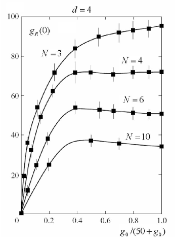
Figure 2: The renormalized charge $g_{R}(0)$ (estimated for zero momenta) against the bare charge $g_{0}$ (corresponding to interatomic spacing $a$) in four-dimensional $\phi^{4}$ theory for fixed values of $Na$ and $m$ but different number $N^{4}$ of lattice sites (according to [11]).

More close inspection reveals that all results for finite $g_{0}$ correspond to the parabolic portion of the $\beta$-function  and do not manifest essential deviations from Eq. 1, while the points for $g_{0}=\infty$ were obtained by reducing to the Ising model, which is an ambiguous procedure.

In fact, two definitions of triviality were hopelessly mixed in the literature (see Sec. 8). As a result, to the end of 20-th century a conviction in triviality of $\phi^{4}$ theory and QED became predominated in literature. Below we overview the comparatively new results [12]–[19] obtained after 2000, which prove the absence of true triviality for these theories.

It is clear from preceding discussion that solution of the ”zero charge” problem needs calculation of the Gell-Mann – Low function $\beta(g)$ at arbitrary $g$, and in particular its asymptotic behavior for $g\to\infty$. Approaches to this problem are discussed in the next sections. Summation of the perturbation series for $\beta(g)$ with the use of the Lipatov asymptotics gives the positive $\beta$-function in four-dimensional $\phi^{4}$ theory and its asymptotic behavior $g^{\alpha}$ with $\alpha\approx 1$ (Sec. 2). The same result for $\alpha$ is obtained in dimensions $d=2$ and $d=3$. The arising hypothesis $\beta(g)\sim g$ for the asymptotic behavior is confirmed in the zero-dimensional case (Sec. 3) and extended to arbitrary dimensions (Sec. 4). The same approach allows to obtain the $\beta$-function in QED (Sec. 5). The problem of complex-valuedness of the bare coupling constant is discussed in Sec. 6 and a scheme without complex parameters is formulated. The latter involves the explicit lattice regularization and reveals the surprising property in renormalizability of $\phi^{4}$ theory: the continual limit in the renormalized theory does not demand the continual limit in the bare theory. This property allows to give a final solution of the triviality problem (Sec. 8) and makes it possible to use high-temperature expansions for calculation of the $\beta$-function with good precision (Sec. 7). The character of renormalizability discovered for $\phi^{4}$ theory is shown to have a general character (Sec. 9), which can be applied to justification of the Wilson theory of confinement (Sec. 10).

Let consider the typical problem in field theory applications. A certain quantity $W(g)$ is given by its formal perturbation expansion

$$W(g)=\sum\limits_{N=0}^{\infty}\,W_{N}(-g)^{N}$$

in powers of the coupling constant $g$. The coefficients $W_{N}$ are given numerically and have the factorial asymptotics at $N\to\infty$,

$$W_{N}^{as}=c_{0}a_{0}^{N}\Gamma(N+b_{0})\,,$$

which is a typical result obtained by the Lipatov method [20]. We want to find $W(g)$ for arbitrary $g$ while the radius of convergence for (4) is zero.

The standard summation procedure is based on the Borel transformation: each term is divided and multiplied by $N!$, the factorial in the numerator is replaced by the definition of the gamma-function, then summation and integration are interchanged,

$$W(g)=\sum\limits_{N=0}^{\infty}W_{N}g^{N}=\sum\limits_{N=0}^{\infty}\frac{W_{N}}{N!}\int\limits_{0}^{\infty}dx\,x^{N}{\rm e}^{-x}g^{N}=\int\limits_{0}^{\infty}dx\,{\rm e}^{-x}\sum\limits_{N=0}^{\infty}\frac{W_{N}}{N!}(gx)^{N}\quad,$$

and we have a series with a factorially improved convergence. We can use $\Gamma(N+b)$ with arbitrary $b$ instead $N!$ and obtain the general Borel–Leroy transformation:

$$W(g)=\int\limits_{0}^{\infty}dxe^{-x}x^{b-1}B(gx)\,,\qquad$$

$$B(z)=\sum\limits_{N=0}^{\infty}B_{N}(-z)^{N}\,,\qquad B_{N}=\frac{W_{N}}{\Gamma(N+b)}\,.$$

The function $W(g)$ is related with its Borel transform $B(z)$ by some integral transformation, while $B(z)$ is given by a series with a factorially improved convergence.

It is easy to show that the Borel transform $B(z)$ has a singularity at the point $z=-1/a_{0}$ (Fig. 3, $a$) determined by the parameter $a_{0}$ in the Lipatov asymptotics (5). The series for $B(z)$ is convergent in the disk $|z|<1/a_{0}$, while we should know it on the positive semi-axis, in order to perform integration in the Borel integral (6); so we need analytical continuation of $B(z)$. Such analytical continuation is easy if the coefficients $W_{N}$ are defined by some simple formula, but it is a problem when they are given numerically.

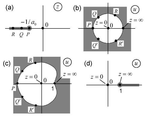
Figure 3: ($a$) The Borel transform $B(z)$ is analytical in the complex plane with the cut $(-\infty,-1/a_{0})$; ($b$) Its domain of analyticity can be conformally mapped to a unit disk in the $u$ plane; ($c$) If analytic continuation is restricted to the positive semi-axis, then a conformal mapping can be made to any domain, for which the point $u=1$ is the nearest to the origin of all boundary points; ($d$) An extreme case of such domain is the $u$ plane with the cut $(1,\infty)$.

The elegant solution of this problem was given by Le Guillou and Zinn-Justin in 1977 [21]. It is based on the hypothesis that in field theory applications all singularities of $B(z)$ lie on the negative semi-axis. This hypothesis can be proved in the case of $\phi^{4}$ theory [22].  If such analytical properties are accepted, we can make a conformal transformation $z=f(u)$, mapping the complex plane with the cut (Fig. 3, $a$) into the unit disk $|u|<1$ (Fig. 3, $b$). If we re-expand $B(z)$ in powers of $u$,

$$B(z)=\sum\limits_{N=0}^{\infty}\left.B_{N}(-z)^{N}\right|_{\displaystyle z=f(u)}\qquad\longrightarrow\qquad B(u)=\sum\limits_{N=0}^{\infty}U_{N}u^{N}\,\,,$$

then such series will be convergent for any $z$. Indeed, all singular points $P,\,Q,\,R,\ldots$ of $B(z)$ lie on the cut, and their images $P,\,Q,\,Q^{\prime},\,R,\,R^{\prime},\ldots$ in the $u$ plane appear on the boundary of the disk $|u|=1$. The re-expanded series in (7) is convergent in the disk $|u|<1$, but the interior of the disk is in the one-to-one correspondence with the analyticity domain in the $z$ plane.

Such conformal mapping is unique (apart from trivial modifications), if we want to make analytical continuation to the whole domain of analyticity. In fact, such strong demand is not necessary since we need $B(z)$ only at the positive semi-axis, in order to produce integration in (6). If we accept that the image of $z=0$ is $u=0$ and the image of $z=\infty$ is $u=1$, then we can make a conformal mapping to any domain, for which the point $u=1$ is the nearest to the origin of all boundary points (Fig. 3, $c$). The series in $u$ converges for $|u|<1$ and particularly in the interval $0<u<1$, which is the image of the positive semi-axis.

Such kind of conformal mapping has advantage in the strong coupling region. A divergency of the series in $u$ is determined by the nearest singular point $u=1$, which is an image of infinity: so the large $N$ behavior of the expansion coefficients $U_{N}$ is related with the strong coupling asymptotics of $W(g)$. In order to diminish influence of other singular points $P,\,Q,\,Q^{\prime},\ldots$, it desirable to move away these points as far, as possible. Thereby, we come to an extremal form of such conformal mapping, when it is made on the whole complex plane with the cut $(1,\infty)$ (Fig. 3, $d$). Mapping of the initial region (Fig. 3, $a$) to the region of Fig. 3, $d$ is given by a simple rational transformation

$$z=\frac{u}{a_{0}(1-u)}\,,$$

for which it is easy to find the relation of $U_{N}$ and $B_{N}$,

$$U_{0}=B_{0}\,,\qquad U_{N}=\sum\limits_{K=1}^{N}\frac{B_{K}}{a_{0}^{K}}(-1)^{K}C_{N-1}^{K-1}\qquad(N\geq 1)\,,$$

where $C_{N}^{K}=N!/K!(N-K)!$ are the binomial coefficients. If $W(g)$ has a power law asymptotics

$$W(g)=W_{\infty}g^{\alpha}\,,\qquad g\to\infty\,,$$

then the large order behavior of $U_{N}$

$$U_{N}=U_{\infty}N^{\alpha-1}\,,\qquad N\to\infty\,,$$

$$U_{\infty}=\frac{W_{\infty}}{a_{0}^{\alpha}\Gamma(\alpha)\Gamma(b+\alpha)}$$

is determined by the parameters $\alpha$ and $W_{\infty}$. Consequently, we come to a very simple algorithm: the coefficients $W_{N}$ of the initial series (4) define the coefficients $U_{N}$ of re-expanded series (7) according to Eqs. 6, 8, while the behavior of $U_{N}$ at large $N$ (Eqs. 10, 11) is related with the strong coupling asymptotics (9) of $W(g)$.

If information on the initial series (4) is sufficient for establishing its strong coupling behavior (9), then summation at arbitrary $g$ presents no problem. The coefficients $U_{N}$ are calculated by Eq. 8 for not very large $N$, and then they are continued according to their asymptotics (10). Consequently, we know all coefficients of the convergent series (7) and it can be summed with required accuracy.

One can apply the described procedure to the perturbation series for the $\beta$-function,

$$\beta(g)=\beta_{2}g^{2}+\beta_{3}g^{3}+\ldots+\beta_{L}g^{L}+\ldots+c_{0}a_{0}^{N}\Gamma(N+b_{0})g^{N}+\ldots\,,$$

having in mind that several first coefficients (till $\beta_{L}$) are known from diagrammatic calculations and their large order behavior is given by the Lipatov method. The intermediate coefficients can be found by interpolation, the natural way for which is as follows. It can be shown that corrections to the Lipatov asymptotics has a form of the regular expansion in $1/N$:

$$\beta_{N}=c_{0}a_{0}^{N}\Gamma(N+b_{0})\left\{1+\frac{A_{1}}{N}+\frac{A_{2}}{N^{2}}+\ldots+\frac{A_{K}}{N^{K}}+\ldots\right\}\,.$$

One can truncate this series and choose the retained coefficients $A_{K}$ from correspondence with the first coefficients $\beta_{2},\ldots,\beta_{L}$; then the interpolation curve goes through the several known points and automatically reaches its asymptotics. To variate this procedure, one can re-expand the series (13) in the inverse powers of $N-\tilde{N}$,

$$\beta_{N}=c_{0}a_{0}^{N}\Gamma(N+b_{0})\left\{1+\frac{\tilde{A}_{1}}{N-\tilde{N}}+\frac{\tilde{A}_{2}}{(N-\tilde{N})^{2}}+\ldots+\frac{\tilde{A}_{K}}{(N-\tilde{N})^{K}}+\ldots\right\}\,,$$

and obtain a set of interpolations, determined by the arbitrary parameter $\tilde{N}$.

In the case of four-dimensional $\phi^{4}$ theory, a realization of this program [12] gives the non-alternating $\beta$-function (Fig. 4, $a$), with the results for the exponent $\alpha$ shown in Fig. 4, $b$.

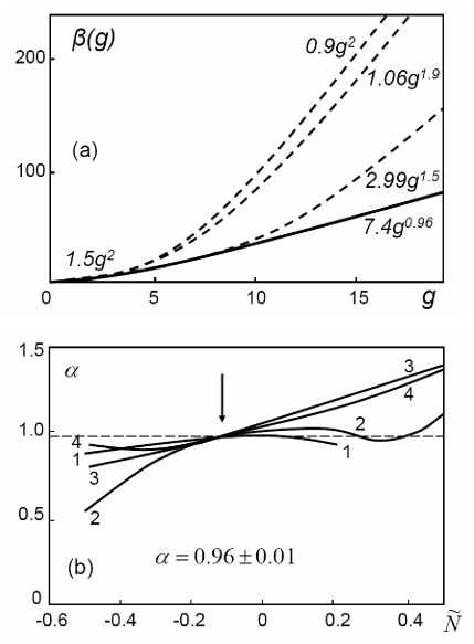
Figure 4: ($a$) General appearance of the $\beta$-function in four-dimensional $\phi^{4}$ theory according to [12] (solid curve), and results obtained by other authors (upper, middle, and lower dashed curves correspond to [26, 27, 28] respectively). ($b$) Different estimations of the exponent $\alpha$ according to [12].

The exponent $\alpha$ is practically independent on $\tilde{N}$, and only its uncertainty depends on this parameter. If we take the result with the minimal uncertainty, we have a value $\alpha=0.96\pm 0.01$, surprisingly close to unity. 

Something close to unity is obtained also in two and three dimensions [29, 30] (Fig. 5).

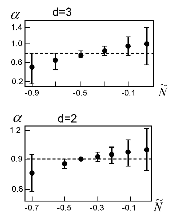
Figure 5: Estimations of the exponent $\alpha$ for $\phi^{4}$ theory in two and three dimensions [29, 30].

The natural hypothesis arises, that $\beta(g)$ has the linear asymptotics

$$\beta(g)\sim g\,\,,\qquad g\to\infty$$

for arbitrary space dimension $d$. If this hypothesis is correct, then there is a natural strategy for its justification:

(i) to test it in a simple case $d=0$;

(ii) to find out the mechanism leading to this asymptotics;

(iii) to generalize this mechanism for arbitrary $d$.

Surprisingly, this program can be realized and Eq. 15 is our main result. Since summation of the series gives non-alternating $\beta(g)$ (Fig. 4, $a$), we may conclude that the second possibility of the Bogoliubov and Shirkov classification is realized.

3. ”Naive” zero-dimensional limit

Consider the $O(n)$-symmetric $\phi^{4}$ theory with the action

$$S\{\phi\}=\int\,d^{d}x\left\{{\textstyle\frac{1}{2}}\sum_{\alpha}(\nabla\phi_{\alpha})^{2}+{\textstyle\frac{1}{2}}m_{0}^{2}\sum_{\alpha}\phi_{\alpha}^{\,2}+{\textstyle\frac{1}{8}}u\left(\sum_{\alpha}\phi_{\alpha}^{\,2}\right)^{2}\right\}\,,$$

$$u=g_{0}\Lambda^{\epsilon}\,,\qquad\epsilon=4-d$$

in $d$–dimensional space; here $m_{0}$ is a bare mass, $\Lambda$ is a momentum cut-off, $g_{0}$ is a dimensionless bare charge. It will be essential for us, that the $\beta$-function can be expressed in terms of the functional integrals . The general functional integral of $\phi^{4}$ theory

$$Z^{(M)}_{\alpha_{1}\ldots\alpha_{M}}(x_{1},\ldots,x_{M})=\int D\phi\,\phi_{\alpha_{1}}(x_{1})\phi_{\alpha_{2}}(x_{2})\ldots\phi_{\alpha_{M}}(x_{M})\exp\left(-S\{\phi\}\right)\,$$

contains $M$ factors of $\phi$ in the pre-exponential; this fact is indicated by subscript $M$.

We can take a zero-dimensional limit, considering the system restricted spatially in all directions. If its size is sufficiently small, we can neglect the spatial dependence of $\phi(x)$ and omit the terms with gradients in Eq. 17; interpreting the functional integral as a multi-dimensional integral on a lattice, we can take the system sufficiently small, so it contains only one lattice site. Consequently, the functional integrals transfer to the ordinary integrals:

$$Z^{(M)}_{\alpha_{1}\ldots\alpha_{M}}=\int d^{n}\phi\,\phi_{\alpha_{1}}\ldots\phi_{\alpha_{M}}\exp\left(-{\textstyle\frac{1}{2}}m_{0}^{2}\phi^{2}-{\textstyle\frac{1}{8}}u\phi^{4}\right)\,.$$

This is the usual understanding of zero-dimensional theory. Such model allows to calculate any quantities with zero external momenta. If external momenta are not zero, the model is not complete: it does not allow to calculate the momentum dependence. To have a closed model, we can accept that there is no momentum dependence at all . This ”naive” model is internally consistent but does not correspond to the true zero-dimensional limit of $\phi^{4}$ theory . The latter fact is not essential for us, since this model is used only for illustration and the proper consideration of the general $d$-dimensional case will be given in the next section.

Expressing $\beta$-function in terms of functional integrals, we obtain it in the form of parametric representation

$$g=1-\frac{n}{n+2}\frac{K_{4}K_{0}}{K_{2}^{2}}$$

$$\beta=-\frac{2n}{n+2}\frac{K_{4}K_{0}}{K_{2}^{2}}\left[2+\frac{\frac{K_{6}K_{0}}{K_{4}K_{2}}-1}{1-\frac{K_{4}K_{0}}{K_{2}^{2}}}\right]\,.$$

The right hand sides of these formulas contain the integrals

$$K_{M}(t)=\int_{0}^{\infty}\phi^{M+n-1}d\phi\,\exp\left(-t\phi^{2}-\phi^{4}\right)\,,\qquad t=\left(\frac{2}{u}\right)^{1/2}\,m_{0}^{2}\,$$

obtained from (18) by simple transformations. According to (19, 20), the quantities $g$ and $\beta$ are functions of the single parameter $t$; excluding $t$ we obtain the dependence $\beta(g)$.

Investigation of (19, 20) for real $t$ shows that $g$ and $\beta$ as functions of $t$ have a behavior shown in Fig. 6, $a$; a combination of these results shows that $\beta(g)$ behaves as in Fig. 6, $b$.

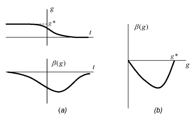
Figure 6: ($a$) Dependence of $g$ and $\beta(g)$ on the parameter $t$. ($b$) A resulting appearance of $\beta(g)$.

We see that variation of the parameter $t$ along the real axis determines $\beta(g)$ in the finite interval $0\leq g\leq g^{*}$ where

$$g^{*}=\frac{2}{n+2}\,\,.$$

To advance into the large $g$ region, we should consider the complex values of $t$.

It appears, that in the complex $t$ plane we should be interested in zeroes of the integrals $K_{M}(t)$. The origin of these zeroes is very simple. There are two saddle points in the integral $K_{M}(t)$, the trivial and nontrivial,

$$\phi_{c1}=0\,,\qquad\phi_{c2}=\sqrt{-t/2}\,,$$

and $K_{M}(t)$ can be presented as a sum of two saddle point contributions:

$$K_{M}(t)=A{\rm e}^{i\psi}+A_{1}{\rm e}^{i\psi_{1}}\,.$$

If these two contributions compensate each other, then the integral can turn to zero. Such compensation can be obtained by adjustment of the complex parameter $t=|t|e^{i\chi}$, and in fact there are infinite number of zeroes lying close to lines $\chi=\pm 3\pi/4$ and accumulating at infinity (Fig. 7).

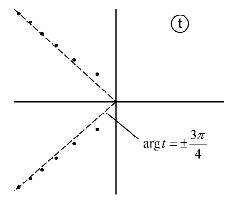
Figure 7: Zeroes of the integrals $K_{M}(t)$ in the complex $t$ plane.

The above saddle-point considerations can be rigorously justified for zeroes lying in the large $|t|$ region. In fact, it is only essential for us that (i) zeroes of $K_{M}(t)$ exist in principle, and (ii) zeroes of different integrals lie in different points.

Now return to the parametric representation (19, 20). It appears, that large values of $g$ can be achieved only near the root of the integral $K_{2}$. If $K_{2}$ tends to zero, then (19, 20) are simplified,

$$g\approx-\frac{n}{n+2}\frac{K_{4}K_{0}}{K_{2}^{2}}\,,\qquad\beta(g)\approx-\frac{4n}{n+2}\frac{K_{4}K_{0}}{K_{2}^{2}}\,,$$

and the parametric representation is resolved in the form

$$\beta(g)=4g\,,\qquad g\to\infty\,.$$

We see that, indeed, the asymptotic behavior of $\beta(g)$ appears to be linear.

The same ideas can be applied to the general $d$-dimensional case. First of all, the actual functional integrals can turn to zero by the same reason. Indeed, the complex values of $t$ with large $|t|$ correspond to complex $g_{0}$ with small $|g_{0}|$ (see Eq. 21), and we come to miraculous conclusion: large values of the renormalized charge $g$ corresponds not to large values of the bare charge $g_{0}$ (as naturally to think ), but to its complex values; more than that, it is sufficient to consider the region $|g_{0}|\ll 1$, where the saddle-point approximation is applicable. As a result, the zeroes of the functional integrals can be obtained by compensation of the saddle-point contributions of the trivial vacuum and of the instanton configuration with the minimal action; contributions of higher instantons are inessential for $|g_{0}|\ll 1$.

Now we need representation of the $\beta$-function in terms of functional integrals. The Fourier transform of (17) will be denoted as $K_{M}$ after extraction of the $\delta$-function of momentum conservation and a factor $I_{\alpha_{1}\ldots\alpha_{M}}$ depending on tensor indices:

$$Z^{(M)}_{\alpha_{1}\ldots\alpha_{M}}(p_{i})=K_{M}(p_{i})\,I_{\alpha_{1}\ldots\alpha_{M}}\,N\delta_{p_{1}+\ldots+p_{M}}$$

where $N$ is the number of sites on the lattice, and $I_{\alpha_{1}\ldots\alpha_{M}}$ is a sum of terms like $\delta_{\alpha_{1}\alpha_{2}}\delta_{\alpha_{3}\alpha_{4}}\ldots$ with all possible pairings. In general, integrals $K_{M}(p_{i})$ are taken at zero momenta, and only the integral $K_{2}$ should be known for small momentum

$$K_{2}(p)=K_{2}-\tilde{K}_{2}p^{2}+\ldots$$

Expressing the $\beta$-function in terms of functional integrals, we have a parametric representation (see [15] for details):

$$g=-\left(\frac{K_{2}}{\tilde{K}_{2}}\right)^{d/2}\frac{K_{4}K_{0}}{K_{2}^{2}}\,,$$

$$\beta=\left(\frac{K_{2}}{\tilde{K}_{2}}\right)^{d/2}\left\{-d\frac{K_{4}K_{0}}{K_{2}^{2}}+2\frac{(K^{\prime}_{4}K_{0}+K_{4}K^{\prime}_{0})K_{2}-2K_{4}K_{0}K^{\prime}_{2}}{K_{2}^{2}}\frac{\tilde{K}_{2}}{K_{2}\tilde{K}^{\prime}_{2}-K^{\prime}_{2}\tilde{K}_{2}}\right\}$$

If $g_{0}$ and $\Lambda$ are fixed, then the right hand sides of these equations are functions of only $m_{0}$, while dependence on the specific choice of $g_{0}$ and $\Lambda$ is absent due to general theorems [31].

We see from Eq. 29 that large values of $g$ can be obtained near the root of either $K_{2}$, or $\tilde{K}_{2}$. If $\tilde{K}_{2}\to 0$, equations (29, 30) are simplified, so $g$ and $\beta$ are given by the same expression apart from the factor $d$,

$$g=-\left(\frac{K_{2}}{\tilde{K}_{2}}\right)^{d/2}\frac{K_{4}K_{0}}{K_{2}^{2}}\,,\qquad\beta=-d\left(\frac{K_{2}}{\tilde{K}_{2}}\right)^{d/2}\frac{K_{4}K_{0}}{K_{2}^{2}}\,,$$

and the parametric representation is resolved as

$$\beta(g)=dg\,,\qquad g\to\infty\,.$$

For $K_{2}\to 0$, the limit $g\to\infty$ can be achieved only for $d<4$:

$$\beta(g)=(d-4)g\,,\qquad g\to\infty\,.$$

The results (32), (33) correspond to different branches of the analytical function $\beta(g)$. It is easy to understand that the physical branch is the first of them. Indeed, it is well known from the phase transitions theory that properties of $\phi^{4}$ theory change smoothly as a function of space dimension, and results for $d=2,\,3$ can be obtained by analytic continuation from $d=4-\epsilon$. According to all available information, the four-dimensional $\beta$-function is positive, and thus has a positive asymptotics; by continuity, the positive asymptotics is expected for $d<4$. The result (32) does obey these demands, while the branch (33) does not exist for $d=4$ at all. Eq. 32 agrees with the approximate results discussed in Sec. 2 and with the exact asymptotic result $\beta(g)=2g$, obtained for the 2D Ising model [33] from the duality relation .

5. Calculation of $\beta$-function in QED

The same ideas can be applied to quantum electrodynamics. Summation of the perturbation series for QED [13] gives the non-alternating $\beta$-function (Fig. 8)

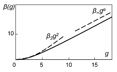
Figure 8: General appearance of the $\beta$-function in QED [13].

with the asymptotics $\beta_{\infty}g^{\alpha}$, where (Fig. 9)

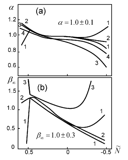
Figure 9: Different estimations of the parameters $\alpha$ and $\beta_{\infty}$ for QED according to [13].

$$\alpha=1.0\pm 0.1\,,\qquad\beta_{\infty}=1.0\pm 0.3\,$$

($g=e^{2}$ is the running fine structure constant). Within uncertainty, the obtained $\beta$-function satisfies inequality

$$0\leq\beta(g)<g\,,$$

established in [34, 35] from the spectral representations, while asymptotics (34) corresponds to the upper bound of (35). Such coincidence is hardly incident and indicates that asymptotics $\beta(g)=g$ is an exact result. We shall see below that it is so indeed.

The general functional integral of QED contains $M$ photon and $2N$ fermionic fields in the pre-exponential,

$$I_{M,2N}=\int DAD\bar{\psi}D\psi\,A_{\mu_{1}}(x_{1})\ldots A_{\mu_{M}}(x_{M})\,\psi(y_{1})\bar{\psi}(z_{1})\ldots\psi(y_{N})\bar{\psi}(z_{N})\exp\left(-S\{A,\psi,\bar{\psi}\}\right)\,,$$

where $S\{A,\psi,\bar{\psi}\}$ is the Euclidean action,

$$S\{A,\psi,\bar{\psi}\}=\int d^{4}x\left[\frac{1}{4}(\partial_{\mu}A_{\nu}-\partial_{\nu}A_{\mu})^{2}+\bar{\psi}(i\!\!\not{\!\partial}-m_{0}+e_{0}\!\not{\!\!A})\psi\right]\,,$$

while $e_{0}$ and $m_{0}$ are the bare charge and mass. The Fourier transforms of the integrals $I_{M,N}$ with excluded $\delta$-functions of the momentum conservation will be referred as $K_{MN}(q_{i},p_{i})$ after extraction of the usual factors depending on tensor indices ; $q_{i}$ and $p_{i}$ are momenta of photons and electrons.

In general, these functional integrals are taken for zero momenta, but two integrals $K_{02}(p)$ and $K_{20}(q)$ should be estimated with the lowest order momentum corrections: the first is linear in $p$, and the second is quadratic in $q$,

$$K_{02}(p)=K_{02}+\tilde{K}_{02}\!\!\not{\!p}\,,\qquad K_{20}(q)=K_{20}+\tilde{K}_{20}q^{2}\,,\qquad$$

and in fact the tilde denotes their momentum derivatives.

Expressing the $\beta$-function in terms of functional integrals (see [16] for details), we have a parametric representation

$$g=-\frac{K_{12}^{2}K_{00}}{\tilde{K}_{02}^{2}\tilde{K}_{20}}\,,\qquad$$

$$\beta(g)=\frac{1}{2}\frac{K_{02}\tilde{K}_{02}}{K_{02}\tilde{K}^{\prime}_{02}-K^{\prime}_{02}\tilde{K}_{02}}\frac{K_{12}^{2}K_{00}}{\tilde{K}_{02}^{2}\tilde{K}_{20}}\left\{\frac{2\,K^{\prime}_{12}}{K_{12}}+\frac{K^{\prime}_{00}}{K_{00}}-\frac{2\,\tilde{K}^{\prime}_{02}}{\tilde{K}_{02}}-\frac{\tilde{K}^{\prime}_{20}}{\tilde{K}_{20}}\right\}$$

According to Secs. 3, 4, the strong coupling regime for renormalized interaction is related with a zero of a certain functional integral. It is clear from (39) that the limit $g\to\infty$ can be realized by two ways: tending to zero either $\tilde{K}_{02}$ or $\tilde{K}_{20}$. For $\tilde{K}_{02}\to 0$, equations (39, 40) are simplified,

$$g=-\frac{K_{12}^{2}K_{00}}{\tilde{K}_{02}^{2}\tilde{K}_{20}}\,,\qquad\beta(g)=-\frac{K_{12}^{2}K_{00}}{\tilde{K}_{02}^{2}\tilde{K}_{20}}\,,$$

and the parametric representation is resolved in the form

$$\beta(g)=g\,,\qquad g\to\infty\,.$$

For $\tilde{K}_{20}\to 0$, one has

$$\beta(g)\propto g^{2}\,,\qquad g\to\infty\,.$$

Consequently, there are two possibilities for the asymptotics of $\beta(g)$, either (42) or (43). The second possibility is in conflict with inequality (35), while the first one is in excellent agreement with results (34) obtained by summation of the perturbation series. In our opinion, it is a sufficient reason to consider (42) as an exact result for asymptotical behavior of the $\beta$-function. It means that the fine structure constant in pure QED behaves as $g\propto L^{-2}$ at small distances.

6. A scheme without complex parameters

Our use of the complex bare parameters may look suspicious, since it corresponds to the non-Hermitian bare Hamiltonian; at first glance, it violates unitarity, since the $S$-matrix is expressed through the Dyson $T$-exponential of the bare action.

In fact, a problem is solved by Bogoliubov’s construction of the axiomatical $S$-matrix [4]: according to it, the general form of the $S$-matrix is given by the $T$-exponential of $iA$, where $A$ is a sum of (i) the bare action, and (ii) a sequence of arbitrary ”integration constants” which are determined by quasi-local operators. In the regularized theory we can set the ”integration constants” to be zero, and the $S$-matrix is determined by the bare action. However, in the course of renormalization these constants are taken non-zero, in order to remove divergences. These non-zero ”integration constants” can be absorbed by the action due to the change of its parameters. As a result, for the true continual theory the $S$-matrix is determined by the renormalized Lagrangian, which is Hermitian for real $g$.

Nevertheless, scientific community has a bias against complex bare parameters: it is related with the old discussion between Lee and Pauli, moderated by Heisenberg, on the exactly solvable model suggested by Lee [36]. After paper [37], the Lee model was considered as unsatisfactory due to existence of ”ghost states”, and this point of view was included in many textbooks. Quite recently [38] it was found that this point of view is incorrect and the Lee model is completely acceptable. A key idea of [38] is that the complex-valued Hamiltonian can be made Herminian by modification of the inner product for the corresponding Hilbert space.

Below we can calm sceptic spirits and suggest a scheme without complex parameters. In this case we accept explicitly the lattice regularization and take the action in the form

$$S\{\phi\}={\textstyle\frac{1}{2}}a^{d}\sum_{\bf x,x^{\prime}}J_{\bf x-x^{\prime}}\phi_{\bf x}\phi_{\bf x^{\prime}}+{\textstyle\frac{1}{2}}m_{0}^{2}a^{d}\sum_{\bf x}\phi_{\bf x}^{2}+{\textstyle\frac{1}{4}}g_{0}a^{2d-4}\sum_{\bf x}\phi_{\bf x}^{4}\,,$$

where we accept $\Lambda=a^{-1}$ ($a$ is a lattice spacing) and restrict ourselves by the case $n=1$. Making a change of variables

$$\phi\longrightarrow\phi\left(g_{0}a^{2d-4}/4\right)^{-1/4}$$

and setting $t=(1/g_{0})^{1/2}$ as before, we can write the functional integral (17) in the form

$$Z^{(M)}\{{\bf x}_{i}\}=(2t)^{\frac{{\cal N}+M}{2}}\int\left(\prod_{\bf x}\,d\phi_{\bf x}\right)\phi_{{\bf x}_{1}}\ldots\phi_{{\bf x}_{M}}\exp\left\{-t\sum_{\bf x,x^{\prime}}J_{\bf x-x^{\prime}}\phi_{\bf x}\phi_{\bf x^{\prime}}-tm_{0}^{2}\sum_{\bf x}\phi_{\bf x}^{2}-\sum_{\bf x}\phi_{\bf x}^{4}\right\}.$$

We accept $a=1$ measuring $J_{\bf x-x^{\prime}}$ and $m_{0}^{2}$ in units of $\Lambda^{2}$. We consider $t$ as a running parameter of the parametric representation and investigate a singularity at $t\to 0$, which has a simple origin. For $g_{0}\gg 1$, Eq. 46 allows expansion over the gradient term $tJ_{\bf x-x^{\prime}}\phi_{\bf x}\phi_{\bf x^{\prime}}$. In zero order in $t$ the integral $Z^{(2)}$ has a $\delta$-functional form in the coordinate representation, $Z^{(2)}({\bf x},{\bf x^{\prime}})\sim\delta_{{\bf x}{\bf x^{\prime}}}$, and its Fourier transform has no momentum dependence; the latter appears only in the first order in $t$. As a result, the integral $\tilde{K}_{2}$ in expansion (28) is small in comparison with $K_{2}$, i.e. $K_{2}/\tilde{K}_{2}\sim 1/t$, which leads to a singularity at $t=0$ in (29, 30). This singularity is more complicated than other singularities in the $t$ plane (Fig.7) and needs the accurate investigation.

Expansion of the functional integral (46) in powers of $t$ expresses it in terms of ordinary integrals

$$I_{2k}=\int_{-\infty}^{\infty}d\phi\,\phi^{2k}\exp\left\{-tm_{0}^{2}\phi^{2}-\phi^{4}\right\}\,$$

and parametric representation (29, 30) reduces to the form

$$g=\left(\frac{n}{2t}\,\frac{I_{0}}{I_{2}}\right)^{d/2}\left(1-\frac{n}{n\!+\!2}\frac{I_{4}I_{0}}{I_{2}^{2}}\right)\,,$$

$$\frac{\beta(g)}{g}=d+2\,\frac{\displaystyle\frac{I_{6}I_{2}}{I_{0}^{2}}-\frac{2I_{4}^{2}}{I_{0}^{2}}+\frac{I_{2}^{2}I_{4}}{I_{0}^{3}}}{\displaystyle\left(\frac{I_{4}}{I_{0}}-\frac{n\!+\!2}{n}\frac{I_{2}^{2}}{I_{0}^{2}}\right)\left(\frac{I_{2}^{2}}{I_{0}^{2}}-\frac{I_{4}}{I_{0}}\right)}\,.$$

This result can be written in a simple form, if the functions $g_{zero}(t)$ and $\beta_{zero}(t)$ are introduced, which correspond to the zero-dimensional case and have appearance shown in Fig.6,$a$:

$$g=\left(\frac{n}{2t}\,\frac{I_{0}}{I_{2}}\right)^{d/2}g_{zero}(tm_{0}^{2})\,,$$

$$\beta(g)=\left(\frac{n}{2t}\,\frac{I_{0}}{I_{2}}\right)^{d/2}\left[dg_{zero}(tm_{0}^{2})+\beta_{zero}(tm_{0}^{2})\right]\,,$$

Resolving the parametric representation in the limit $t\to 0$, we come to the asymptotics

$$\beta(g)=\left[d+\frac{\beta_{zero}(0)}{g_{zero}(0)}\right]\,g\,,\qquad g\to\infty$$

reducing to the result $\beta(g)=2.29\,g$ of the paper [39] after substitution of numerical values. However, this result is not final. Instead of the limit $t\to 0$ for fixed $m_{0}$ one can consider a limiting transition under condition $tm_{0}^{2}\to const$ with different values of $const$; then the general structure of theory remains unchanged, but asymptotical behavior of $\beta(g)$ will be different. The question arises on the correct character of the limiting transition, corresponding to the strong coupling regime.

The gradient expansions of the considered type was exploited in a number of works [39]-[42], and ambiguity of a strong coupling limit was finally realized by their authors. Nevertheless, the correct character of the limiting transition was not established till the paper [17]. In the framework of the parametric representation (29, 30) the indicated problem accepts the different form. Deficiency of the result (49) consists in the presence of two independent parameters $t$ and $tm_{0}^{2}$. If one of them is excluded in favor of $g$, then the $\beta$-function depends not only on $g$ but also on $m_{0}^{2}$, while the latter dependence should be absent according to general theorems [31]. The question arises on resolving of this contradiction. Of course, there is no real contradiction, because the general theorems suggest that the continual limit $\Lambda\to\infty$ is already taken. Physically it means a fulfilment of the condition

$$m^{2}\ll\Lambda^{2}\,,$$

which is equivalent to the condition $\xi\gg a$ for the correlation length $\xi$; it means that a characteristic scale of the field variation contains many lattice sites, so further diminishing of $a$ is of no significance.

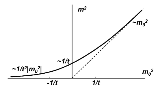
Figure 10: The renormalized mass as a function of the bare mass in the strong coupling region.

As a result of the gradient expansions, the renormalized mass is represented in the form (Fig.10)

$$m^{2}=\frac{K_{2}}{\tilde{K}_{2}}=\frac{n}{2t}\,\frac{I_{0}}{I_{2}}=\left\{\begin{array}[]{cc}m_{0}^{2}\,,&tm_{0}^{2}\gg 1\\ {}\hfil\\ \sim 1/t\,,&|tm_{0}^{2}|\mathbin{\lower 3.0pt\hbox{$\hbox to0.0pt{\raise 5.0pt\hbox{$\char 60\relax$}\hss}\mathchar 29208\relax$}}1\\ {}\hfil\\ \sim 1/t^{2}|m_{0}^{2}|\,,&-tm_{0}^{2}\gg 1\,,\end{array}\right.$$

and the condition $m^{2}\ll 1$ (corresponding to (50) in dimensional units) is satisfied in the case

$$tm_{0}^{2}=-\kappa\,,\qquad\kappa\gg 1\,.$$

After replacement $\phi_{{\bf x}}^{2}\to\kappa\phi_{{\bf x}}^{2}/2$ the exponential in (46) accepts a form

$$\exp\left\{-{\textstyle\frac{1}{2}}t\kappa\,\sum_{\bf x,x^{\prime}}J_{\bf x-x^{\prime}}\phi_{\bf x}\phi_{\bf x^{\prime}}\right\}\prod_{\bf x}\exp\left\{{\textstyle\frac{1}{4}}\kappa^{2}\left(2\phi_{\bf x}^{2}-\phi_{\bf x}^{4}\right)\right\}$$

where the last factor is localized near $\phi^{2}_{\bf x}=1$ and can be replaced by $A\delta(\phi^{2}_{\bf x}-1)$. The constant $A$ is inessential for a ratio of two integrals and one can set $A=1$. As a result, Eq. 46 accepts a form

$$Z_{M}\{{\bf x}_{i}\}=(t\kappa)^{\frac{{\cal N}+M}{2}}\int\left(\prod_{\bf x}\,d\phi_{\bf x}\right)\phi_{{\bf x}_{1}}\ldots\phi_{{\bf x}_{M}}\exp\left\{-{\textstyle\frac{1}{2}}t\kappa\,\sum_{\bf x,x^{\prime}}J_{\bf x-x^{\prime}}\phi_{\bf x}\phi_{\bf x^{\prime}}\right\}\prod_{\bf x}\delta(\phi^{2}_{\bf x}-1)$$

and a functional integral transforms into the Ising sum over values $\phi_{\bf x}=\pm 1$. In the $n$-component case one obtains a $\sigma$-model [43] instead of the Ising model.

Now all functional integrals depend on the single variable $t\kappa$ and the right-hand sides of (29, 30) are functions of only this argument; it defines the $\beta$-function depending only on $g$. In the physical motivation of the limiting transition we implied the conditions providing (50)

$$t\ll 1\,,\qquad\kappa\gg 1\,,\qquad t\kappa\gg 1\,,$$

but in fact only first two inequalities were used in derivation of (54). Therefore, transformation to the Ising model is valid under conditions

$$t\ll 1\,,\qquad\kappa\gg 1\,,\qquad t\kappa\quad\mbox{is arbitrary}\,.$$

In particular, it is valid in the region $t\kappa\ll 1$, where gradient expansions are possible and large values of the renormalized charge $g$ are reached. Using (51, 52), we come to conclusion that strong coupling regime of $\phi^{4}$ theory corresponds to the limit

$$t\to 0\,,\qquad tm_{0}^{2}\to-\infty\,,\qquad tm^{2}\to 0\,,\qquad m^{2}\to\infty\,,$$

so neither $m_{0}=const$ nor $m=const$ is the correct condition for a limiting transition. It means that dependencies of Fig.2 are not actual from the very beginning.

Returning to (49) and setting $-tm_{0}^{2}=\kappa\gg 1$, we have

$$g=\left(\frac{n}{t\kappa}\right)^{d/2}g^{*}\,,\qquad\beta(g)=\left(\frac{n}{t\kappa}\,\right)^{d/2}dg^{*}\,,$$

and so the asymptotics of the $\beta$-function is obtained

$$\beta(g)=dg\,\qquad(g\to\infty)\,,$$

coinciding with (32). We see that singularity at $t=0$ leads to the same result as singularities at the complex values of $t$.

Representation (54) for functional integrals can be used for calculation of the observable quantities. The latter are obtained in the form

$$A_{obs}=\Lambda^{d_{A}}f_{A}(t\kappa)\,,$$

where $d_{A}$ is a physical dimension of the quantity $A_{obs}$. Using analogous expressions for $g$ and $m$,

$$g=f_{g}(t\kappa)\,,\qquad m^{2}=\Lambda^{2}f_{m}(t\kappa)\,,$$

we can rewrite (59) in the form

$$A_{obs}=m^{d_{A}}F(g)\,,$$

which does not contained the bare parameters $g_{0}$, $m_{0}$, $\Lambda$; so (61) gives a ”theorem of renormalizability” for a strong coupling region. It should be stressed that we do not take the continual limit in the bare theory and retain the lattice as a convenient instrument for representation of functional integrals, and only the lattice spacing $a$ is excluded from the physical results.

7. Application of high temperature expansions

Rewriting (56) in dimensional quantities and changing $t\kappa\to\kappa$, we see that reducing of $\phi^{4}$ theory to the Ising model is possible under conditions

$$g_{0}\gg 1\,,\qquad-g_{0}^{-1/2}m_{0}^{2}/\Lambda^{2}\gg 1\,,\qquad-g_{0}^{-1}m_{0}^{2}/\Lambda^{2}=\kappa\,,$$

where $\kappa$ is an arbitrary parameter having a sense of the inverse temperature in the Ising model. Correspondingly, Eqs. 48 have a structure

$$g=F(\kappa)\,,\qquad\beta(g)=F_{1}(\kappa)\,,$$

and define the $\beta$-function in the parametric form. At first glance, the condition $g_{0}\gg 1$ corresponds to the strong coupling regime and parametric representation (63) is limited only by this regime. However, there is another view on this situation. Let strengthen conditions (62) by taking the limit

$$g_{0}\to\infty\,,\qquad-g_{0}^{-1/2}m_{0}^{2}/\Lambda^{2}\to\infty\,,\qquad-g_{0}^{-1}m_{0}^{2}/\Lambda^{2}=\kappa$$

In this case, transition from (46) to (54) is valid without any approximations and conserves a strict equivalence with the initial $\phi^{4}$ theory under a certain choice of its bare parameters. The last property conserves a form of the Lagrangian under renormalizations. The taken limit $g_{0}\to\infty$ does not mean the same limit for the renormalized charge $g$; in fact, according to gradient expansions, $g$ varies from infinity to the order of unity when $\kappa$ changes from zero to a finite value. Since parametric representation (63) is exact and specifies the $\beta$ function in the interval $1\mathbin{\lower 3.0pt\hbox{$\hbox to0.0pt{\raise 5.0pt\hbox{$\char 60\relax$}\hss}\mathchar 29208\relax$}}g<\infty$, it can be analytically continued and treated as a definition of $\beta(g)$ at arbitrary values of $g$. However, a certain doubt arises: does this definition provide the correct results in the weak-coupling region?

An answer to this question can be obtained using high-temperature series [44]. Such series are traditionally constructed for quantities (superscript $c$ marks the connected diagrams)

$$\raisebox{2.0pt}{$\chi$}_{2}=\sum_{\bf x}\langle\phi_{{\bf x}}\phi_{{\bf 0}}\rangle^{c}\,,\qquad\raisebox{2.0pt}{$\mu$}_{2}=\sum_{\bf x}{\bf x}^{2}\langle\phi_{{\bf x}}\phi_{{\bf 0}}\rangle^{c}\,,\qquad\raisebox{2.0pt}{$\chi$}_{4}=\sum_{\bf x,y,z}\langle\phi_{{\bf x}}\phi_{{\bf y}}\phi_{{\bf z}}\phi_{{\bf 0}}\rangle^{c}\,,\qquad$$

which coincides up to factors with the ratios $K_{2}/K_{0}$, $\tilde{K}_{2}/K_{0}$, and $K_{4}/K_{0}$ of the functional integrals specified above; more precisely,

$$\frac{K_{2}}{\tilde{K}_{2}}\,=\,2d\,\frac{\raisebox{2.0pt}{$\chi$}_{2}}{\raisebox{1.0pt}{$\mu$}_{2}}\,\equiv\frac{1}{\kappa}f_{0}(\kappa)\,,$$

$$\frac{K_{2}}{K_{0}}\,=\,2\kappa\,\raisebox{2.0pt}{$\chi$}_{2}\equiv\kappa f_{2}(\kappa)\,,$$

$$\frac{K_{4}K_{0}}{K_{2}^{2}}\,=\,\frac{1}{3}\,\frac{\raisebox{2.0pt}{$\chi$}_{4}}{\raisebox{2.0pt}{$\chi$}_{2}^{2}}\,\equiv-f_{4}(\kappa)\,,$$

where the introduced functions $f_{i}(\kappa)$ will be used below. It was taken into account that there is no zeroth term in the expansion of ${\raisebox{1.0pt}{$\mu$}_{2}}$ in $\kappa$ (see Eq. 68 below), so that all functions $f_{0}(\kappa)$, $f_{2}(\kappa)$, and $f_{4}(\kappa)$ are regular and their expansions begin with the zeroth term. The substitution of (66) into (29, 30) gives

$$g=\left(\frac{f_{0}(\kappa)}{\kappa}\right)^{d/2}f_{4}(\kappa)\,,\qquad\frac{\beta(g)}{g}=d-2\kappa\,\frac{[\ln f_{4}(\kappa)]^{\prime}}{1-\kappa\,[\ln f_{0}(\kappa)]^{\prime}}\,.$$

The initial parametric representation (29, 30) for the $\beta$-function is ”dead”, since evaluation of functional integrals looks hopeless. It becomes ”alive” in the form (67), since functions $f_{i}(\kappa)$ can be calculated using high-temperature expansions .

For a simple hypercubic lattice with the interaction between the nearest neighbors, the first terms of the expansion for functions (65) have the form (in the case $d=4$, $n=1$) [45]

$$\raisebox{2.0pt}{$\chi$}_{2}=1+16\kappa+224\kappa^{2}+\ldots$$

$$\raisebox{1.0pt}{$\mu$}_{2}=16\kappa+512\kappa^{2}+33920/3\kappa^{3}+\ldots$$

$$\raisebox{2.0pt}{$\chi$}_{4}=-2-128\kappa-4672\kappa^{2}-\ldots$$

Taking limit $\kappa\to 0$, it is easy to obtain the strong coupling behavior for the $\beta$-function and anomalous dimensions [18], and then develop their expansion in powers of $g^{-2/d}$. Below, 14 terms of expansion (68) are used, which are given for $n=1$ in tables 5, 8, and 11 of the paper [45].

The use of Pade-approximants allows to obtain the $\beta$-function and anomalous dimensions at arbitrary $g$. The general strategy consists in the following. The Ising model has a phase transition in a certain point $\kappa_{c}=1/T_{c}$, and a typical physical quantity $F(\kappa)$ has the critical behavior of the form

$$F\propto(T-T_{c})^{-\lambda}\propto(\kappa_{c}-\kappa)^{-\lambda}\,.$$

If $F(\kappa)$ is expanded in $\kappa$, then a convergence radius of the expansion is limited by the quantity $\kappa_{c}$; in actual cases, $\kappa_{c}$ is the nearest singularity to the coordinate origin. If the logarithmic derivative of $F$ is taken,

$$(\ln F)^{\prime}=\frac{F^{\prime}}{F}=\frac{{-\lambda}}{\kappa-\kappa_{c}}+\mbox{less singular terms}\,,$$

then the main singularity for it is a simple pole with a residue ${-\lambda}$ and can be investigated using the Pade approximation [46]. The Pade-approximant $[M/N]$ is defined as the ratio of two polynomials of degrees $M$ and $N$,

$$(\ln F)^{\prime}=\,\frac{P_{M}(\kappa)}{Q_{N}(\kappa)}\,=\,\frac{p_{0}+p_{1}\kappa+\ldots+p_{M}\kappa^{M}}{1+q_{1}\kappa+\ldots+q_{N}\kappa^{N}}\,\,,$$

whose coefficients are chosen to reproduce the first $M+N+1$ coefficients in the expansion of $(\ln F)^{\prime}$ over $\kappa$. It is known that Pade-approximants successfully predict the nearest singularities of the corresponding function if these singularities are the simple poles [44, 46] . If $\lambda$ and $\kappa_{c}$ are predicted reliably, then the whole function $F(\kappa)$ can be found in the interval $0\leq\kappa\leq\kappa_{c}$ with a good precision. If such results for $f_{i}(\kappa)$ are substituted into the right-hand sides of (67), then the $\beta$-function can be determined in the interval $g^{*}\leq g<\infty$, where $g^{*}$ is the fixed point of the renormalization group. In the four-dimensional case, one has $g^{*}=0$ and $\beta(g)$ is completely determined by the described procedure.

The use of this strategy in the four-dimensional case is complicated by the existence of logarithmic corrections to scaling [47, 31]:

$$\raisebox{2.0pt}{$\chi$}_{2}\sim\tau^{-1}|\ln\tau|^{p}\,,\qquad\xi^{2}\sim\frac{\raisebox{1.0pt}{$\mu$}_{2}}{\raisebox{2.0pt}{$\chi$}_{2}}\sim\tau^{-1}|\ln\tau|^{p}\,,\qquad\raisebox{2.0pt}{$\chi$}_{4}\sim\tau^{-4}|\ln\tau|^{4p-1}\,,$$

where $\tau\sim(\kappa_{c}-\kappa)$ is a distance to the transition and $p=(n+2)/(n+8)$. Substitution to (66, 67) gives for behavior of charge $g$

$$g=\frac{c_{0}}{|\ln\tau|}\,,\qquad c_{0}=2/\beta_{2}\qquad(\tau\to 0)\,,$$

where the coefficient of the logarithmic factor is universal. If equations (72) and (73) are fulfilled, then the parametric representation (67) automatically reproduces the one-loop result of weak-coupling expansion for the $\beta$-function.

The objective test of Eqs. 72 for lattice models were performed in many works [48]–[58]. In particular, it was convincingly shown in [48, 49] that high-temperature series for the Ising model allow reliable prediction of the exponent $p$. Eq. 73 was confirmed with a satisfactory accuracy in [49, 51]. Already these results provide the positive answer to the question formulated above: parametric representation (63) gives correct results for the $\beta$-function in the weak-coupling region.

The modified treatment procedure suggested in [18] allows to improve estimation of the constant $c_{0}$, which was not very satisfactory in preceding papers. The relation $\tau=A_{0}(1-\kappa/\kappa_{c})$ contains the non-universal coefficient $A_{0}$ which is essential in logarithmic factors. If such factors are extracted from functions (65) in accordance with (72) and the Pade analysis is applied to remaining functions, then strong coupling estimations of the constant $c_{0}$ (Fig.11,$a$) are close to the

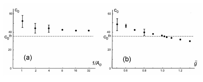
Figure 11: The constant $c_{0}$ in Eq. 73 versus $A_{0}$ in the leading logarithmic approximation ($a$), and versus $\bar{g}$ in the next-to-leading logarithmic approximation ($b$).

theoretical value $c_{0}^{th}=35.09$ but systematically exceed it. If the logarithmic factors are extracted in accordance with the next-to-leading logarithmic approximation, then estimations of $c_{0}$ improve (Fig.11,$b$) and become close to the theoretical value in the same range $0.85\div 1.06$ of the non-universal parameter $\bar{g}$ (analogous to $A_{0}$) where the power law singularities of remaining factors are close to theoretical expectations. The exact $c_{0}$ value is realized at $\bar{g}\approx 1.02$, and this value of $\bar{g}$ can be used in the further analysis. Extracting from the quantities $\raisebox{2.0pt}{$\chi$}_{2}$, $\raisebox{2.0pt}{$\mu$}_{2}$, $\raisebox{2.0pt}{$\chi$}_{4}$ all logarithmic and power-law singularities and applying the Pade-approximation to remaining regular functions, one can calculate the right hand sides of (67) for the whole interval $0<\kappa<\kappa_{c}$ and obtain the $\beta$-function at arbitrary $g$ (see a solid line in Fig.12). To give an impression on accuracy of the calculation, we show by the dotted line the analogous dependence obtained under the assumption of the constancy of indicated regular functions, when any information on them is dropped from results. In fact, these regular functions are known with the accuracy of several percents.

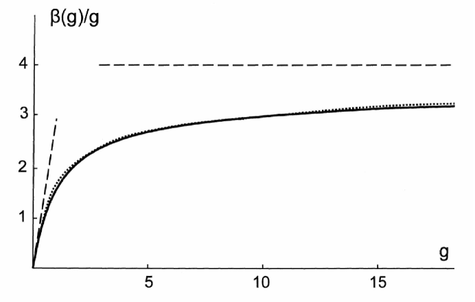
Figure 12: A solid line is a calculated function $\beta(g)/g$. The dashed lines are the strong- and weak-coupling asymptotic behaviors. A dotted line shows the same results obtained under the assumption of the constancy of regular functions.

Analogously, one can obtain a behavior of the renormalized charge $g$ and the renormalized mass $m$ as functions of $\kappa$ (Fig.13), which is essential for characterization of the lattice $\phi^{4}$ theory.

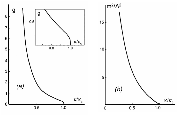
Figure 13: Renormalized charge $g$ ($a$) and mass $m$ ($b$) versus $\kappa/\kappa_{c}$.

8. Is $\phi^{4}$ theory trivial?

In the preceding sections we have established, that the Gell-Mann – Low function $\beta(g)$ in four-dimensional $\phi^{4}$ theory is non-alternating and has asymptotic behavior $\beta(g)=4g$ at $g\to\infty$. According to the Bogoliubov and Shirkov classification (Sec. 1), it means a possibility to construct the continuous theory with finite interaction at large distances. This conclusion is in visible contradiction with lattice results indicating triviality of $\phi^{4}$ theory.

As we stressed in Sec. 1, one should differ two definitions of triviality. Wilson triviality means that integration of equation (3) in the direction of large distances $L$ gives the effective charge $g$ tending to zero; this definition implies the massless theory, since in the opposite case the distance scale is saturated by the inverse mass. In definition of true triviality one considers the massive theory and suggests finite interaction $g_{\infty}$ for $L\mathbin{\lower 3.0pt\hbox{$\hbox to0.0pt{\raise 5.0pt\hbox{$\char 62\relax$}\hss}\mathchar 29208\relax$}}m^{-1}$; a theory is trivial, if integration of (3) in direction of small $L$ gives a divergency at finite $L_{0}$ and does not allow to reach the $L\to 0$ limit. Such situation is internally inconsistent and means incorrectness of the initial suggestion on finite interaction at large distances; in fact, $L_{0}\to 0$ if $g_{\infty}\to 0$. Wilson triviality means that $\beta$-function is non-negative and has a zero only for $g=0$. True triviality needs in addition its sufficiently quick growth at infinity, $\beta(g)\sim g^{\alpha}$ with $\alpha>1$. According to preceding sections, $\phi^{4}$ theory and QED are trivial in the Wilson sense, but do not possess true triviality.

Two definitions of triviality were hopelessly mixed in literature [10], and there are two main reasons for that. Firstly, it is rather difficult to test true triviality in the lattice approach . Secondly, one can advance arguments that give an illusion of equivalence of two definitions. As illustration to the latter point, consider the following reasoning. The only alternative to perturbative approach is to express all quantities in terms of the functional integrals. The latter depend on the bare charge $g_{0}$, bare mass $m_{0}$ and the ultraviolet cut-off $\Lambda$. Taking into account their dimensional character, one has the following relations for the renormalized charge $g$, renormalized mass $m$ and observable quantities $A_{i}$

$$g=F_{g}\left(g_{0},m_{0}/\Lambda\right)\,,\qquad$$

$$m=\Lambda F_{m}\left(g_{0},m_{0}/\Lambda\right)\,,\qquad$$

$$A_{i}=\Lambda^{d_{i}}F_{i}\left(g_{0},m_{0}/\Lambda\right)\,,\qquad$$

where $d_{i}$ is a physical dimensionality of $A_{i}$. Excluding $g_{0}$ and $m_{0}/\Lambda$ in favor of $g$ and $m/\Lambda$, one has

$$A_{i}=m^{d_{i}}\tilde{F}_{i}\left(g,m/\Lambda\right)\,.\qquad$$

To eliminate the dependence on $\Lambda$ we should take the limit $m/\Lambda\to 0$. In the lattice approach, this limit corresponds to $\xi/a\to\infty$, i.e. to the phase transition point. The latter is determined by a zero of $\beta$-function, which gives $g=0$ in four-dimensional $\phi^{4}$ theory.

In this argumentation, Wilson triviality is considered as given, while true triviality is ”derived” from it. Of course, such ”proof” is incorrect, because two definitions are surely not equivalent. This shortcoming originates from our assumption that a generic situation takes place in Eq. 75, and a limit $m/\Lambda\to 0$ is necessary. However, the special case is possible, when the $m/\Lambda$ dependence is absent in (75), and a limiting transition is irrelevant. This special case fills the ”gap” between two definitions and makes them not equivalent.

According to Sec. 6, such special case is actually realized in $\phi^{4}$ theory. Let return to Eqs. 74 and impose the condition $m\ll\Lambda$, corresponding to the continuum limit of renormalized theory. If this condition is imposed in the region $g_{0}\gg 1$, then $\phi^{4}$ theory reduces to the Ising model, containing the single parameter $\kappa$, which plays the role of inverse temperature; relations (74) accept the form

$$g=F_{g}\left(\kappa\right)\,,\qquad$$

$$m=\Lambda F_{m}\left(\kappa\right)\,,\qquad$$

$$A_{i}=\Lambda^{d_{i}}F_{i}\left(\kappa\right)\,.\qquad$$

So far there is nothing unusual: the condition $m/\Lambda\to 0$ gives a relation between $g_{0}$ and $m_{0}/\Lambda$, so all functions in Eq. 74 depend on the single parameter, which we denoted as $\kappa$. The non-trivial point consists in the fact that condition $m/\Lambda\ll 1$ is sufficient for transformation to the Ising model, but not necessary for it. This transformation is possible under the weaker conditions, which are compatible with an arbitrary value of $m/\Lambda$ (Sec. 6). Excluding $\kappa$ from (76), one obtains the equations

$$A_{i}=m^{d_{i}}F_{i}\left(g\right)\,,\qquad$$

which are analogous to (75), but do not contain the parameter $m/\Lambda$. As a result, the program of renormalization is completely fulfilled, and no additional limiting transitions are necessary. It means that (a) we can retain the lattice in the bare theory (as a convenient tool for representation of functional integrals), and (b) relation between $m$ and $\Lambda$ (or $\xi$ and $a$) can be arbitrary, so a finite value of $g$ becomes possible.

Usually, the lattice theory contains more parameters than the initial field theory. For example, in discretization of the gradient term of $\phi^{4}$ theory we obtain a set of the overlap integrals $J_{x}$, which can be chosen rather arbitrary. Then an interesting question arises: if we can retain a lattice in the bare theory, then what lattice model should be chosen?

The answer can be found from Eq. 75. Since dependence on $m/\Lambda$ is absent, we can tend this ratio to zero. But in this limit (when $\xi/a\to\infty$) there are physical grounds for independence of functions $F_{i}$ on the way of cut-off. If such independence takes place for $m/\Lambda\to 0$, it retains for arbitrary $m/\Lambda$ due to independence of functions $F_{i}$ on this parameter. In fact, this argumentation implies renormalizability of theory (due to which the dependence on $\Lambda$ can be excluded) and belonging of the lattice model to the proper universality class (inside of which the dependence on the way of cut-off is absent).

The lattice theory is frequently considered as a reasonable approximation to the true field theory. In this case we should accept the condition $\xi\gg a$, which signifies that one has a lot of lattice sites on the characteristic scale of variation of field. This condition can be strengthen till $\xi/a\to\infty$ or liberalized till $\xi\mathbin{\lower 3.0pt\hbox{$\hbox to0.0pt{\raise 5.0pt\hbox{$\char 62\relax$}\hss}\mathchar 29208\relax$}}a$. The first case corresponds to the point of phase transition and gives $g=0$. In the second case we obtain restriction $g\mathbin{\lower 3.0pt\hbox{$\hbox to0.0pt{\raise 5.0pt\hbox{$\char 60\relax$}\hss}\mathchar 29208\relax$}}1$ (for the proper charge normalization [18]), which can be used to obtain the upper bound on the Higgs mass [45, 59].

In fact, the lattice theory should not be considered as any approximation to field theory, though it is possible for $g_{0}\ll 1$. The true field theory is continuous from the very beginning and does not contain any lattice. The lattice is present only in the bare theory, which is an auxiliary construction and is completely removed later. No physical requirements, like $\xi\gg a$, are relevant for it. If one removes the condition $\xi\gg a$, then any values of $g$ become admissible . In fact, a real designation of the bare theory is to represent the relations between physical quantities in the parametric form (74). Such representation has no deep sense already due to its ambiguity: it can be written in many different forms, changing $g_{0}$ and $m_{0}/\Lambda$ by any other pair of variables.

We see that contradiction between the continual and lattice approaches is resolved by a special character of renormalizability in $\phi^{4}$ theory: correct relations (77) between physical quantities can be obtained for the arbitrary value of the parameter $a/\xi$, while a dependence on this parameter is absent; to obtain the continuous renormalized theory, there is no need to eliminate a lattice from the bare theory.

9. General situation in renormalizable theories

The interesting question arises: is such kind of renormalizability related with the specific properties of $\phi^{4}$ theory, or it is a manifestation of some general mechanism?

We shall see below that the second variant is correct. It can be understood in the framework of Wilson’s many-parameter renormalization group (RG) [5]. According to it, the parameters $p_{i}$ of some lattice Hamiltonian are considered as functions of the length scale ${\it l}$.  The flow of these parameters is determined by the RG equations, which can be written in the differential form

$$-\frac{dp_{i}}{d\ln({\it l}/a)}=F_{i}\{p_{k}\}\,.$$

These equations can be linearized near the fixed point

$$p_{i}({\it l})=p^{*}_{i}\qquad\mbox{ (\,for\quad all\quad{\it l\,})}$$

and investigated by the standard methods of linear algebra. The ordinary phase transitions are described by the saddle points of such equations. The simplest saddle point in the two-parameter space has the straight-line trajectories in two main directions (one stable and one unstable), while the rest of trajectories are hyperbolic. For the usual phase transitions, there are infinite number of stable directions and one (in the simplest case) unstable direction. The latter is related with some controlling parameter like temperature, measuring the distance to the critical point.

Instead of increasing ${\it l}$ for fixed $a$, we can diminish $a$ for fixed ${\it l}$. The continuum limit $a\to 0$ of field theory corresponds to the critical surface $\xi/a=\infty$ in the many-parameter space (Fig.14).

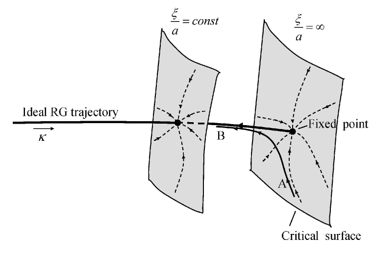
Figure 14: Schematic of the Wilson many-parameter space.

All trajectories on the critical surface tend to the fixed point. The unstable trajectory, originating at the fixed point will be referred as an ”ideal RG trajectory”: along it one has the exact one-parameter scaling, which is a pipe dream in many fields of physics (see e.g. [60]). To define it rigorously, let consider the limit $a\to 0$ with fixed $\xi/a$; then all trajectories lying at the surface $\xi/a=const$ (Fig.14) tend to one point (analogously to the critical surface), while the locus of such points is the ideal RG trajectory.

Let the parameter $\kappa$ is measuring the distance along the ideal trajectory: then $\xi/a$ (or $\Lambda/m$) is a function of $\kappa$. Analogously, all dimensionless quantities depend only on $\kappa$, while the dimensional quantities are measured in units of $\Lambda$. As a result, we come to equations

$$g=F_{g}\left(\kappa\right)\,,\qquad m=\Lambda F_{m}\left(\kappa\right)\,,\qquad A_{i}=\Lambda^{d_{i}}F_{i}\left(\kappa\right)\,,$$

which coincide with (76) and give the relations (77) without dependence on $m/\Lambda$.

The above construction has a following sense. If the limit $a\to 0$ is taken in the arbitrary manner, then the system will go to infinity along the unstable direction and appear far from the critical surface, which is our goal. Therefore, we suggest to take the continual limit in two steps:

(a) take a limit $a\to 0$ for $a/\xi=const$;

(b) take a limit $a/\xi\to 0$.

It appears, that dependence on $a$ in relations (77) disappears already at the first step. The second step becomes unnecessary and there is no need to take the continuum limit in the bare theory . The $const$ appearing in (a) is one of the possible definitions of the parameter $\kappa$.

Any RG trajectory is a line of ”constant physics”, since the RG transformation is simply a mental construction and does not affect the large-scale properties of the system. All trajectories belonging to the critical surface and terminated in the fixed point, give the equivalent lattice representations for the unique continuous field theory; another equivalent representation is given by the ideal RG trajectory originating from the fixed point. Consider the trajectory $AB$, which begins near the critical surface and goes along it, and then tends to the ideal RG trajectory (Fig.14). Introducing $\tilde{\kappa}$ as a distance along $AB$, we come to the parametric representation analogous to (80) and relations (77), following from it. The latter relations will be the same as obtained from (80), since in both cases they are independent of $\xi/a$ and correspond to the physically equivalent models for $\xi/a=0$ and $\xi/a=\infty$. We can retain definition of $\kappa$ as a distance along the ideal trajectory, and assign it to the point of $AB$, corresponding to the same value of $\xi/a$. Writing relations analogous to (80)

$$g=\tilde{F}_{g}\left(\kappa\right)\,,\qquad m=\Lambda F_{m}\left(\kappa\right)\,,\qquad A_{i}=\Lambda^{d_{i}}\tilde{F}_{i}\left(\kappa\right)\,,$$

we see that the second relation remained unchanged, but the rest of them become different. The charge $g$ usually belongs to irrelevant parameters and we can introduce ”the axis of charges” on the critical surface; using trajectories of $AB$ type with different directions relative to ”the axis of charges” we can obtain different functions $g=\tilde{F}_{g}(\kappa)$. It means that the functional relation between $g$ and $\kappa$ becomes indeterminate and can be omitted.

As a result, the renormalized and bare sectors of theory become decoupled. The renormalized sector contains relations (77), where $g$ and $m$ are considered as independent variables. The bare sector contains only relation $a/\xi=m/\Lambda=F_{m}\left(\kappa\right)$, which determines $\kappa$ as a function of $a$ and is irrelevant from viewpoint of physics. Parameter $a/\xi$ becomes absolutely free.

Thereby, we come to the following conclusion: renormalizable theory of the considered type allows representation in the form of lattice theory, which gives the correct relations between physical quantities, and contains free parameter $a/\xi$, which does not enter these relations.

Consider a pure Yang-Mills theory, i.e. QCD without quarks. Then the quark mass does not enter as a parameter and the theory contains no natural mass scale. To avoid the specific difficulties related with such situation, we introduce the ”extended version” of Yang-Mills theory, where the role of the bare mass $m_{0}$ (more exactly, the ratio $m_{0}/\Lambda$) is played by some auxiliary parameter $p$ characterizing the lattice theory; as a renormalized mass, we accept the mass $m$ of the lightest glueball (the bound state of several gluons), while the correlation length $\xi$ is defined as $m^{-1}$. Thereby, two bare parameters $g_{0}$ and $p$ provide the observable values for renormalized $g$ and $m$. In order to return to the standard variant of theory, we should remove the introduced extra degree of freedom by fixing one relation between observable quantities. However, it can be done on the late stage (see below), while the main of analysis is produced for the ”extended version”. The latter is analogous to $\phi^{4}$ theory.

According to Wilson [62], confinement can be proved in the lattice version of the Yang-Mills theory for large values of the bare charge $g_{0}$. The energy of interaction for two probe quarks separated by a distance $R$ is $V(R)=\sigma R$, while the string tension $\sigma$ and the glueball mass $m$ are given by expressions [61, 62, 63]

$$\sigma=\frac{\ln(3g_{0}^{2})}{a^{2}}\,,\qquad m=\frac{4\,\ln(3g_{0}^{2})}{a}\,.$$

In spite of the evident success, the Wilson theory is considered as purely illustrative and having no relation to real QCD. As was indicated by Wilson himself, his theory corresponds to a situation

$$\xi\ll a\qquad\mbox{ or}\qquad m\gg\Lambda\,,$$

which is considered as nonphysical. An attempt to advance into the physical region inevitably destroys the strong coupling regime. Indeed, the $\beta$-function in terms of the bare charge is believed to be negative [64, 65], and $g_{0}$ tends to zero in the continuum limit $a\to 0$. Therefore, the strong coupling regime is inevitably destroyed in the physical region $\xi/a\mathbin{\lower 3.0pt\hbox{$\hbox to0.0pt{\raise 5.0pt\hbox{$\char 62\relax$}\hss}\mathchar 29208\relax$}}1$ and Wilson’s theory becomes inapplicable.

A situation changes drastically, if we use representation (76, 77) introduced in the previous sections. In this case:

(i) due to absence of the $\xi/a$ dependence in (77), this parameter can be taken arbitrary: it eliminates objections against the nonphysical regime in Wilson’s theory.

(ii) there is no direct relation between the bare and renormalized charge; rewriting the second expression (82) in the form

$$g_{0}^{2}=\frac{1}{3}\exp\left(\frac{ma}{4}\right)=\frac{1}{3}\exp\left\{\frac{a}{4\xi}\right\}\,,$$

we see that, independently of renormalized values of $g$ and $m$, it is possible to choose the free parameter $a/\xi$ so as to obtain a sufficiently large value for $g_{0}$. Then Wilson’s theory becomes applicable and the first relation (82) gives a finite value for $\sigma$, i.e. confinement.

Representation (76, 77) cannot be introduced for the simplest Wilson action [61, 62, 63], since it does not contain a sufficient number of parameters. To obtain the observable values of $\sigma$ and $m$ one should fix both $g_{0}$ and $a$; but the fixed $a$ means impossibility to introduce a representation with free parameter $a/\xi$. This problem can be easily solved using more complicated forms of the action [61]. As a result, we obtain instead of (82)

$$\sigma=\frac{\ln(3g_{0}^{2})}{a_{1}^{2}}\,,\qquad m=\frac{4\,\ln(3g_{0}^{2})}{a_{2}}\,,$$

where $a_{1}=k_{1}a$, $a_{2}=k_{2}a$ simply by dimensional reasons [19].

Relation (77) in application to $\sigma$ has a form

$$\sigma=m^{2}F_{\sigma}(g)\,,$$

so $g$ is functionally related with $\sigma/m^{2}$. On the other hand, Eqs. 85 give

$$\frac{\sigma}{m^{2}}=\frac{a_{2}^{2}}{16a_{1}^{2}\,\ln(3g_{0}^{2})}\,,$$

and the ratio $\sigma/m^{2}\,$ changes from a finite value till zero in the strong coupling region $g_{0}\mathbin{\lower 3.0pt\hbox{$\hbox to0.0pt{\raise 5.0pt\hbox{$\char 62\relax$}\hss}\mathchar 29208\relax$}}1$. It means that only restricted range of $g$ values can be reproduced. Such restriction is natural due to the physical essence of the problem. Indeed, the linear confinement potential is expected only at large distances, where $g$ is certainly not small; hence, small values of $g$ are inaccessible in the Wilson regime. Contrary, the restricted range of $\sigma/m^{2}$ values goes across the logic of theory. Indeed, $a/\xi$ is a free parameter and all physical results can be obtained at its arbitrary value. In the case $a/\xi\gg 1$, the regime of confinement is controlled analytically and any physically accessible value of $\sigma/m^{2}$ should be possible in this limit. In fact, the range of $\sigma/m^{2}$ values can be extended if we use the models with essentially different $a_{1}$ and $a_{2}$ [19]. Absence of restrictions on $\sigma/m^{2}$ in the presence of restrictions on $g$ is possible only if dependence $\sigma/m^{2}=F_{\sigma}(g)$ is singular (Fig.15); fortunately, we can demonstrate that it is a probable variant.

Investigations of complicated lattice versions of Yang-Mills theory [61] show existence of phase transitions (lying in the region $g_{0}\sim 1$), corresponding to vanishing of the lightest glueball mass $m$, with finite values of $\sigma$ and other mass parameters. These transitions are considered as lattice artifacts, since they do not survive in the continuum limit, when $g_{0}\to 0$. In our approach the limit $a\to 0$ is not necessary and such phase transitions acquire the physical sense. If $m$ vanishes at the point $g=g^{*}$, then dependence $\sigma/m^{2}=F_{\sigma}(g)$ has a form shown in Fig.15.

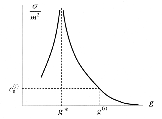
Figure 15: Dependence of $\sigma/m^{2}$ against $g$. In order to obtain the special values $c^{(i)}_{0}$, corresponding to zero values of the mass gap, one should mark all stable fixed points $g^{(i)}$ on the horizontal axis and make a construction shown in the figure.

Existence of points with $m=0$ in the parametric space means that the ”extended version” of Yang-Mills theory does not possess the mass gap. To eliminate this defect, we should return to the standard variant of theory, fixing one relation between the observable quantities. The character of such relations is well-known and is determined by ”dimensional transmutation” [61, Sec. 14.1], [66, Sec. IV.6], according to which all quantities of the same dimensionality differ only by the constant factor, independent of $g_{0}$. For our purposes it is convenient to accept the condition

$$\sigma/m^{2}=c\,,$$

which defines the one-parameter family of Yang-Mills theories with different values of the structural constant $c$. Under condition (88), the points with $m=0$, $\sigma=const$ become inaccessible.

It does not yet prove the existence of a mass gap, since $\sigma$ and $m$ can vanish simultaneously. In order to analyze such situations, consider the Gell-Mann – Low equation for the renormalized charge $g$ attributed to the length scale $m^{-1}$

$$\frac{d\,g^{2}}{d\,\ln m^{2}}=\beta(g^{2})=\beta_{0}g^{4}+\beta_{1}g^{6}+\ldots\,,$$

where $\beta$-function does not coincide with that of the bare theory, but has the same first coefficients $\beta_{0}$ and $\beta_{1}$. It is clear that the value $g^{*}$ (Fig.15) is a root of the $\beta$-function; generally, it has several roots determining the RG fixed points. In the limit $m\to 0$, the charge $g$ tends to one of these fixed points, while following variants are possible for $\sigma/m^{2}$: (a) $\sigma/m^{2}\to\infty$, (b) $\sigma/m^{2}\to 0$, (c) $\sigma/m^{2}\to c_{0}$. The first two variants are incompatible with Eq. 88, while the third variant is possible in the case $c=c_{0}$. If there are several stable fixed points $g^{(i)}$, then there are several special values $c^{(i)}_{0}$ (see Fig.15), for which the mass gap vanishes; for all other values of $c$ the mass gap is finite.

Physically, it looks most probable that only one fixed point $g^{*}$ with $\sigma/m^{2}\to\infty$ is present, so no special values $c^{(i)}_{0}$ arise. Mathematically, one can suggest an infinite number of fixed points, which form a sequence $c^{(i)}_{0}$ everywhere dense in the interval $(0,\infty)$. However, small values of $\sigma/m^{2}$ correspond to the Wilson regime where finiteness of $\sigma$ and $m$ is verified immediately. As a result, the proof of the mass gap is complete for small values of the structural constant $c$.

If quarks with a zero mass  are introduced, then the regime of dimensional transmutation is conserved and the trick with ”extension” of theory remains possible; it seems, that the general structure of theory is also retained.

In conclusion, the properties of continuous Yang-Mills theory can be reproduced by a certain lattice theory. The bare charge $g_{0}$ in this lattice theory can be taken arbitrary, and in particular infinitely large. For large $g_{0}$, any reasonable lattice version of Yang-Mills theory gives finite values of $\sigma$ and $m$. Vanishing of $m$ is possible under exceptional conditions, which are avoided in the general situation. As a result, the problem of analytical proof of confinement and the mass gap can be considered as solved, at least on the physical level of rigor.

11. Conclusion

We have given an overview of field theory evolution from its early stage to the present time. A widespread opinion on triviality of $\phi^{4}$ theory and QED should in fact be revisited. They are trivial in Wilson’s sense, but escape the Landau ”zero-charge” situation. This conclusion is reached by summation of weak-coupling perturbation expansions for $\beta(g)$, analytical calculation of its strong coupling asymptotics, and confirmation of results by analysis of strong coupling expansions. The second possibility in the Bogoliubov and Shirkov classification is shown to be actual, allowing to construct the continuous theory with finite interaction at large distances. A possibility to retain a lattice in the bare theory allows to justify the Wilson approach in theory of confinement.

References

- [1] L. D. Landau, A. A. Abrikosov, and I. M. Khalatnikov, Dokl. Akad. Nauk SSSR 95, 497, 773, 1177 (1954).
- [2] L. D. Landau, I. Ya. Pomeranchuk, Dokl. Akad. Nauk SSSR 102, 489 (1955). I. Ya. Pomeranchuk, Dokl. Akad. Nauk SSSR 103, 1005 (1955).
- [3] Collected papers of L. D. Landau, Pergamon Press, 1965. Articles 84, 100.
- [4] N. N. Bogoliubov and D. V. Shirkov, Introduction to the Theory of Quantized Fields, 3rd ed. (Nauka, Moscow, 1976; Wiley, New York, 1980).
- [5] K. G. Wilson and J. Kogut, Phys. Rep. C 12, 75 (1975).
- [6] K. G. Wilson and M. E. Fisher, Phys. Rev. Lett. 28, 240 (1972). K. G. Wilson, Phys. Rev. Lett. 28, 548 (1972).
- [7] J. P. Eckmann, R. Epstein, Commun. Math. Soc. 64, 95 (1979).
- [8] J. Frolich, Nucl. Phys. B 200 [FS4], 281 (1982).
- [9] M. Aizenman, Commun. Math. Soc. 86, 1 (1982).
- [10] I. M. Suslov, arXiv: 0806.0789.
- [11] B. Freedman, P. Smolensky, D. Weingarten, Phys. Lett. B 113, 481 (1982).
- [12] I. M. Suslov, Zh. Eksp. Teor. Fiz. 120, 5 (2001) [JETP 93, 1 (2001)].
- [13] I. M. Suslov, Pis’ma Zh. Eksp. Teor. Fiz. 74, 211 (2001) [JETP Lett. 74, 191 (2001)].
- [14] I. M. Suslov, Zh. Eksp. Teor. Fiz. 127, 1350 (2005) [JETP 100, 1188 (2005)].
- [15] I. M. Suslov, Zh. Eksp. Teor. Fiz. 134, 490 (2008) [JETP 107, 413 (2008)].
- [16] I. M. Suslov, Zh. Eksp. Teor. Fiz. 135, 1129 (2009) [JETP 108, 980 (2009)].
- [17] I. M. Suslov, Zh. Eksp. Teor. Fiz. 138, 508 (2010) [JETP 111, 450 (2010)].
- [18] I. M. Suslov, Zh. Eksp. Teor. Fiz. 139, 319 (2011). [JETP 112, 274 (2011)].
- [19] I. M. Suslov, Zh. Eksp. Teor. Fiz. 140, 712 (2011) [JETP 113, 619 (2011)].
- [20] L. N. Lipatov, Zh. Eksp. Teor. Fiz. 72, 411 (1977) [Sov.Phys. JETP 45, 216 (1977)].
- [21] J. C. Le Guillou, J. Zinn-Justin, Phys. Rev. Lett. 35, 55 (1977).
- [22] I. M. Suslov, Zh. Eksp. Teor. Fiz. 116, 369 (1999) [JETP 89, 197 (1999)].
- [23] G. ’t Hooft, in: The whys of subnuclear physics (Erice, 1977), ed. A Zichichi, Plenum Press, New York, 1979.
- [24] M. Beneke, Phys. Rept. 317, 1 (1999), Sec. 2.4.
- [25] I. M. Suslov, Zh. Eksp. Teor. Fiz. 126, 542 (2004) [JETP 99, 474 (2004)].
- [26] D. I. Kazakov, O. V. Tarasov, and D. V. Shirkov, Teor.Mat. Fiz. 38, 15 (1979).
- [27] Yu. A. Kubyshin, Teor. Mat. Fiz. 58, 137 (1984).
- [28] A. N. Sissakian, I. L. Solovtsov, and O. P. Solovtsova,Phys. Lett. B 321, 381 (1994).
- [29] A. A. Pogorelov, I. M. Suslov, Zh. Eksp. Teor. Fiz. 132, 406 (2007) [JETP 105, 360 (2007)].
- [30] A. A. Pogorelov, I. M. Suslov, Pis’ma Zh. Eksp. Teor. Fiz. 86, 41 (2007) [JETP Lett. 86, 39 (2007)].
- [31] E. Brezin, J. C. Le Guillou, J. Zinn-Justin, in Phase Transitions and Critical Phenomena, ed. by C. Domb and M. S. Green, Academic, New York (1976), Vol. VI.
- [32] A. A. Vladimirov and D. V. Shirkov, Usp. Fiz. Nauk 129, 407 (1979) [Sov. Phys. Usp. 22, 860 (1979)].
- [33] G. Jug, B. N. Shalaev, J. Phys. A 32, 7249 (1999).
- [34] N .V. Krasnikov, Nucl. Phys. B 192, 497 (1981).
- [35] H. Yamagishi, Phys. Rev. D 25, 464 (1982).
- [36] T. D. Lee, Phys. Rev. 95, 1329 (1954).
- [37] G. Kllen, W. Pauli, Mat.-Fyz. Medd. 30, No.7 (1955).
- [38] C. M. Bender, S. F. Brandt, J. - H. Chen, Q. Wang, Phys. Rev. D 71, 025014 (2005).
- [39] P. Castoldi, C. Schomblond, Nucl. Phys. B 139, 269 (1978).
- [40] C. M. Bender, F. Cooper, G. S. Guralnik, D. H. Sharp, Phys. Rev. D 19, 1865 (1979).
- [41] C. M. Bender, F. Cooper, G. S. Guralnik, R. Roskies, D. H. Sharp, Phys. Rev. D 23, 2976 (1981); 23, 2999 (1981); 24, 2683 (1981).
- [42] R. Benzi, G. Martinelli, G. Parisi, Nucl. Phys. B 135, 429 (1978).
- [43] M. Moshe, J. Zinn-Justin, Phys. Rept. 385, 69 (2003).
- [44] D. S. Gaunt, A. J. Guttmann, in Phase Transitions and Critical Phenomena, ed. by C. Domb and M. S. Green, Academic, New York (1974), Vol. 3.
- [45] M. Lscher, P. Weisz, Nucl. Phys. B 300 325 (1988).
- [46] G. A. Baker, Essentials of Pade-Approximants, Academic, New York, 1975.
- [47] A. I. Larkin and D. E. Khmel’nitskii, Zh. Eksp. Teor.Fiz. 56, 2087 (1969) [Sov. Phys. JETP 29, 1123 (1969)].
- [48] S. Mc Kenzie, M. F. Sykes, D. S. Gaunt, J. Phys. A: Math.Gen. 12, 871 (1979);
- [49] S. Mc Kenzie, D. S. Gaunt, J. Phys. A: Math.Gen. 13, 1015 (1980).
- [50] S. Mc Kenzie, M. F. Sykes, D. S. Gaunt, J. Phys. A: Math.Gen. 12, 743 (1978);
- [51] P. Butera, M. Comi, hep-th/0112225.
- [52] J. K. Kim, A. Patrascioiu, Phys. Rev. D 47, 2588 (1993).
- [53] A. Vladikas, C. C. Wong, Phys. Lett. B 189, 154 (1987).
- [54] R. Kenna, C. B. Lang, Phys. Rev. E 49, 5012 (1994).
- [55] W. Bernreuther, M. Cockeler, M. Kremer, Nucl. Phys.. B 295[FS21], 211 (1988).
- [56] A. J. Guttmann, J. Phys. A: Math.Gen. 11, L103 (1978).
- [57] C. A. de Carvalho, S. Caracciolo, J. Frlich, Nucl. Phys.. B 215[FS7], 209 (1983).
- [58] P. Grassberger, R. Hegger, L. Schafer, J. Phys. A: Math.Gen. 27, 7265 (1994).
- [59] R. F. Dashen, H. Neuberger, Phys. Rev. Lett. 50, 1897 (1983).
- [60] E. Abrahams, P. W. Anderson, D. C. Licciardello, and T. V. Ramakrishman, Phys. Rev. Lett. 42, 673 (1979).
- [61] R. Gupta, arXiv: hep-lat/9807028.
- [62] K. G. Wilson , Phys. Rev. D 10, 2445 (1974).
- [63] M. Creutz, Quarks, gluons and lattices, Cambridge University Press, 1983.
- [64] C. Callan, R. Dashen, D. Gross, Phys. Rev. D 20, 3279 (1979).
- [65] J. B. Kogut, R. B. Pearson, J. Shigemitsu, Phys. Rev. Lett. 43, 484 (1979).
- [66] A. A. Slavnov, L. D. Faddeev. Introduction to Quantum Theory of Gauge Fields (Nauka, Moscow, 1988).