Convergence of sequential Quasi-Monte Carlo smoothing algorithms

Abstract

Gerber and Chopin, (2015) recently introduced Sequential quasi-Monte Carlo (SQMC) algorithms as an efficient way to perform filtering in state-space models. The basic idea is to replace random variables with low-discrepancy point sets, so as to obtain faster convergence than with standard particle filtering. Gerber and Chopin, (2015) describe briefly several ways to extend SQMC to smoothing, but do not provide supporting theory for this extension. We discuss more thoroughly how smoothing may be performed within SQMC, and derive convergence results for the so-obtained smoothing algorithms. We consider in particular SQMC equivalents of forward smoothing and forward filtering backward sampling, which are the most well-known smoothing techniques. As a preliminary step, we provide a generalization of the classical result of Hlawka and Mück, (1972) on the transformation of QMC point sets into low discrepancy point sets with respect to non uniform distributions. As a corollary of the latter, we note that we can slightly weaken the assumptions to prove the consistency of SQMC.

Keywords: Hidden Markov models; Low discrepancy; Particle filtering; Quasi-Monte Carlo; Sequential quasi-Monte Carlo; Smoothing; State-space models.

1 Introduction

State-space models are popular tools to model real life phenomena in many fields such as Economics, Engineering and Neuroscience. These models are mainly used for extracting information about a hidden Markov process $(\mathbf{x}_{t})_{t\geq 0}$ of interest from a set of observations $\mathbf{y}_{0:T}:=(\mathbf{y}_{0},\dots,\mathbf{y}_{T})$. In practice, this typically translates to the estimation of $p(\mathbf{x}_{t}|\mathbf{y}_{0:t})$, the distribution of $\mathbf{x}_{t}$ given the data $\mathbf{y}_{0:t}$, $0\leq t\leq T$ (called the filtering distribution), and/or to $p(\mathbf{x}_{0:T}|\mathbf{y}_{0:T})$ (called the smoothing distribution). However, these distributions are intractable in most cases, and require to be approximated in some way, the most popular being particle filtering (Sequential Monte Carlo). See e.g. the books of Doucet et al., (2001), Cappé et al., (2005) for more background on state-space models and particle filters.

Recently, Gerber and Chopin, (2015) introduced sequential quasi-Monte Carlo (SQMC) as an efficient alternative to particle filtering. Essentially, SQMC amounts to replacing the random variates generated by a particle filter with a QMC (low-discrepancy) point set; that is a set of $N$ points that are selected so as to cover more evenly the space that random variates would; see e.g. the books of Lemieux, (2009), Leobacher and Pillichshammer, (2014) for more background on QMC.

Gerber and Chopin, (2015) established that, for some constructions of RQMC (randomised QMC) point sets, the convergence rate of SQMC (with respect to $N$, the number of simulations) is at worst $\mathcal{O}_{P}(N^{-1/2})$, while it is ${\scriptscriptstyle\mathcal{O}}_{P}(N^{-1/2})$ on the class of continuous and bounded functions. (This of course compares favourably to the $\mathcal{O}_{P}(N^{-1/2})$ rate of particle filtering.) In addition, the numerical results of Gerber and Chopin, (2015) show that SQMC dramatically outperforms particle filtering in several applications.

One important question that remains however is how to use SQMC to obtain smoothing estimates that converge as $N\rightarrow+\infty$. Smoothing is recognised as a more difficult problem than filtering (Briers et al.,, 2010). Smoothing algorithms typically require extra steps on top of particle filtering (such as a backward pass), and often cost $\mathcal{O}(N^{2})$ (but some variants cost $\mathcal{O}(N)$, as discussed later).

This paper discusses existing smoothing algorithms, explains how they may be adapted to SQMC, and presents convergence results for the corresponding SQMC smoothing algorithms. We first study forward smoothing, where trajectories are carried forward in the particle filter, and show that this approach leads to consistent estimates in SQMC. Then, we derive a SQMC version of forward filtering backward sampling (where complete trajectories are simulated from the positions simulated by a particle filter, see Godsill et al.,, 2004), and establish convergence results for the so obtained smoothing estimates. We also consider the marginal version of backward sampling, which usually allows for a more precise estimation of marginal smoothing distributions.

The rest of this paper is organized as follows. Section 2 introduces the model and the notations considered in this work, and give a short description of SQMC. Section 3 contains some preliminary results that will be needed to study SQMC smoothing. We first present a new consistency result for the forward step, which has the advantage to rely on weaker assumptions than in Gerber and Chopin, (2015), and state a result relative to the backward decomposition and SQMC estimation of the smoothing distribution. Then, we provide a generalization of the classical result of Hlawka and Mück, (1972) on the transformation of QMC point sets into low discrepancy point sets with respect to non uniform distributions that is essential to the analysis of QMC smoothing algorithms. This section ends with some results on the conversion of discrepancies through the Hilbert space filling curve. In Section 4 we establish the consistency of QMC forward smoothing while our results on QMC forward-backward smoothing are given Section 5. In Section 6 a numerical study examines the performance of the QMC smoothing strategies discussed in this work while Section 7 concludes.

2 Preliminaries

2.1 Model and related notations

Let $(\mathbf{x}_{t})_{t\geq 0}$ a Markov chain, defined on a space $\mathcal{X}\subseteq\mathbb{R}^{d}$ (equipped with Lebesgue measure), with initial distribution $m_{0}(\mathrm{d}\mathbf{x}_{0})$, transition kernel $m_{t}(\mathbf{x}_{t-1},\mathrm{d}\mathbf{x}_{t})$, $t\geq 1$, and let $(G_{t})_{t\geq 0}$ a sequence of (measurable) potential functions, $G_{0}:\mathcal{X}\rightarrow\mathbb{R}^{+}$, $G_{t}:\mathcal{X}\times\mathcal{X}\rightarrow\mathbb{R}^{+}$. As in Gerber and Chopin, (2015), and most of the QMC literature, we take $\mathcal{X}=[0,1)^{d}$, but see Section 3 of Gerber and Chopin, (2015) for how to generalise our results to unbounded state spaces.

For this Feynman-Kac model $(m_{t},G_{t})_{t\geq 0}$, let $\overline{\mathbb{Q}}_{t}$ and $\mathbb{Q}_{t}$ be the probability measures on $\mathcal{X}$ such that, for any bounded measurable function $\varphi:\mathcal{X}\rightarrow\mathbb{R}$,

$$\overline{\mathbb{Q}}_{t}(\varphi) =\frac{1}{Z_{t-1}}\mathbb{E}\left[\varphi(\mathbf{x}_{t})G_{0}(\mathbf{x}_{0})\prod_{s=1}^{t-1}G_{s}(\mathbf{x}_{s-1},\mathbf{x}_{s})\right]$$

$$\mathbb{Q}_{t}(\varphi) =\frac{1}{Z_{t}}\mathbb{E}\left[\varphi(\mathbf{x}_{t})G_{0}(\mathbf{x}_{0})\prod_{s=1}^{t}G_{s}(\mathbf{x}_{s-1},\mathbf{x}_{s})\right]$$

$$Z_{t} =\mathbb{E}\left[G_{0}(\mathbf{x}_{0})\prod_{s=1}^{t}G_{s}(\mathbf{x}_{s-1},\mathbf{x}_{s})\right]$$

where expectations are with respect to the law of Markov chain $(\mathbf{x}_{t})$, and empty products equal one. Similarly, let $\widetilde{\mathbb{Q}}_{t}$ be the probability measure on $\mathcal{X}^{t+1}$ such that, for any bounded test function $\varphi:\mathcal{X}^{t+1}\rightarrow\mathbb{R}$,

$$\widetilde{\mathbb{Q}}_{t}(\varphi)=\frac{1}{Z_{t}}\mathbb{E}\left[\varphi(\mathbf{x}_{0:t})G_{0}(\mathbf{x}_{0})\prod_{s=1}^{t}G_{s}(\mathbf{x}_{s-1},\mathbf{x}_{s})\right].$$

In the sequel, the notation $0:t$ is used to denote the set of integers $\{0,\dots,t\}$ and $\mathbf{x}_{0:t}$ denotes the collection $\{\mathbf{x}_{s}\}_{s=0}^{t}$. Similarly, in what follows we use the shorthand $\mathbf{x}^{1:N}$ for a collection $\{\mathbf{x}^{n}\}_{n=1}^{N}$ of $N$ points in $\mathbb{R}^{d}$, and $\mathbf{x}_{0:t}^{1:N}$ for collection $\{\mathbf{x}_{0:t}^{n}\}_{n=1}^{N}$ of $N$ points in $\mathbb{R}^{(t+1)d}$. Finally, for a probability measure $\pi\in\mathcal{P}(\mathcal{X})$, with $\mathcal{P}(\mathcal{X})$ the set of probability measures on $\mathcal{X}$ absolutely continuous with respect to the Lebesgue measure, $\pi(\varphi)$ denotes the expectation of $\varphi(\mathbf{x})$ under $\pi$.

To make more transparent the connection between this Feynman-Kac  formulation and state-space models, assume Markov chain $(\mathbf{x}_{t})$ is observed indirectly through $\mathbf{y}_{t}$, which has conditional probability density $f^{Y}(\mathbf{y}_{t}|\mathbf{x}_{t})$ (with respect to an appropriate measure, typically Lebesgue). If we take $G_{0}(\mathbf{x}_{0})=f^{Y}(\mathbf{y}_{0}|\mathbf{x}_{0})$, $G_{t}(\mathbf{x}_{t-1},\mathbf{x}_{t})=f^{Y}(\mathbf{y}_{t}|\mathbf{x}_{t})$ for $t>0$, $\mathbb{Q}_{t}(\mathrm{d}\mathbf{x}_{t})$ becomes the filtering distribution (the law of $\mathbf{x}_{t}|\mathbf{y}_{0:t}$), $\overline{\mathbb{Q}}_{t}(\mathrm{d}\mathbf{x}_{t})$ the predictive distribution (the law of $\mathbf{x}_{t}|\mathbf{y}_{0:t-1}$), and $\widetilde{\mathbb{Q}}_{t}(\mathrm{d}\mathbf{x}_{0:t})$, the object of interest in this work, namely the smoothing distribution (the law of $\mathbf{x}_{0:t}|\mathbf{y}_{0:t}$). In addition, $Z_{t}$ is the marginal likelihood of observations $\mathbf{y}_{0:t}$. In this case, $G_{t}$ depends only on $\mathbf{x}_{t}$, but having a $G_{t}$ that depends on both $\mathbf{x}_{t-1}$ and $\mathbf{x}_{t}$ makes it possible to apply our results to a more general class of algorithms (such as those where the Markov transition used to simulate particles differs from the Markov transition of the model).

2.2 Extreme norm and QMC point sets

As in Gerber and Chopin, (2015), our consistency results are stated in term of the extreme norm, defined, for two probability measures $\pi_{1}$ and $\pi_{2}$ on $[0,1)^{d}$, by

$$\|\pi_{1}-\pi_{2}\|_{\mathrm{E}}=\sup_{B\in\mathcal{B}_{[0,1)^{d}}}\left|\pi_{1}(B)-\pi_{2}(B)\right|$$

where

$$\mathcal{B}_{[0,1)^{d}}=\{B=\prod_{i=1}^{d}[a_{i},b_{i}],\,0\leq a_{i}<b_{i}<1\}.$$

Note that $\|\pi_{N}-\pi\|_{\mathrm{E}}\rightarrow 0$ implies that $\pi_{N}(\varphi)\rightarrow\pi(\varphi)$ for any bounded and continuous function $\varphi$ (by portmanteau lemma, see e.g. Lemma 2.2, p.6 of Van der Vaart, 2007). In words, consistency for the extreme norm implies consistency of estimates for test functions $\varphi$ that are bounded and continuous.

The extreme norm is natural in QMC contexts since it can be viewed as the generalization of the extreme discrepancy of a point set $\mathbf{u}^{1:N}$ in $[0,1)^{d}$, defined by

$$D(\mathbf{u}^{1:N})=\|\mathcal{S}(\mathbf{u}^{1:N})-\lambda_{d}\|_{\mathrm{E}}$$

where $\lambda_{d}$ denotes the Lebesgue measure on $\mathbb{R}^{d}$ and $\mathcal{S}$ is the operator

$$\mathcal{S}:\mathbf{u}^{1:N}\rightarrow\frac{1}{N}\sum_{n=1}^{N}\delta_{\mathbf{u}^{n}}.$$

The extreme discrepancy therefore measures how a point set spreads evenly over $[0,1)^{d}$ and is used to define formally QMC point sets. To be more specific, $\mathbf{u}^{1:N}$ is a QMC point set in $[0,1)^{d}$ if $D(\mathbf{u}^{1:N})=\mathcal{O}(N^{-1}(\log N)^{d})$. Note that, for a sample $\mathbf{u}^{1:N}$ of $N$ IID uniform random numbers in $[0,1)^{d}$, $D(\mathbf{u}^{1:N})=\mathcal{O}(N^{-1/2}\log\log N)$ almost surely by the law of iterated logarithm (see e.g. Niederreiter,, 1992, page 167). There exist many constructions of QMC point sets in the literature (see Niederreiter,, 1992; Dick and Pillichshammer,, 2010, for more details on this topic) and, although we write $\mathbf{u}^{1:N}$ rather than $\mathbf{u}^{N,1:N}$, $\mathbf{u}^{1:N}$ may not necessarily be the $N$ first points of a fixed sequence, i.e. one may have $\mathbf{u}^{N,N-1}\neq\mathbf{u}^{N-1,N-1}$. However, it is worth keeping in mind that all the results presented in this paper hold both for point sets and sequences.

Even if in this work we are mainly interested in consistency results (which hold for deterministic point sets $\mathbf{u}^{1:N}$), we will sometimes refer to randomized QMC (RQMC) point sets. Formally, $\mathbf{u}^{1:N}$ is RQMC point set if it is a QMC point set with probability one and if, marginally, $\mathbf{u}^{n}\sim\mathcal{U}([0,1)^{d})$ for all $n\in 1:N$.

2.3 The Hilbert space-filling curve

The Hilbert space filling curve plays a key role in the construction and the analysis of SQMC. This curve is a Hölder continuous fractal map $H:[0,1]\rightarrow[0,1]^{d}$ that fills completely $[0,1]^{d}$; see Figure 1 for a graphical depiction, and Appendix A for a presentation of its mains properties. In what follows, we denote by $h:[0,1]^{d}\rightarrow[0,1]$ its pseudo-inverse which verifies, for any $\mathbf{x}\in[0,1]^{d}$, $H\circ h(\mathbf{x})=\mathbf{x}$, and, for $d=1$, we use the natural convention that $H$ and $h$ are the identity mappings, i.e. $H(x)=h(x)=x$, $\forall x\in[0,1]$. The Hilbert curve is not uniquely defined; in this work, we assume that $H$ is such that $H(0)=\mathbf{0}\in[0,1]^{d}$ (this is in fact the classical way to construct the Hilbert curve, see e.g. Hamilton and Rau-Chaplin,, 2008). This technical assumption is needed in order to be consistent with the fact that we work with left-closed and right-opened hypercubes since, in that case, $h([0,1)^{d})=[0,1)$.

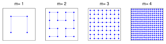
Figure 1: First four iterates of sequence $H_{m}$, the limit of which is the Hilbert curve $H$, for $d=2$ (source: He and Owen, (2014))

2.4 Rosenblatt transform

Another important technical tool for SQMC is the Rosenblatt transform. For a probability distribution $\pi$ over $[0,1)$, $F_{\pi}$ denotes its CDF (cumulative distribution), and $F_{\pi}^{-1}$ its inverse CDF; i.e. $F_{\pi}^{-1}=\inf\{x\in[0,1):\,F(x)\geq u\}$. More generally, for a probability distribution $\pi$ over $\mathcal{X}=[0,1)^{d}$, $F_{\pi}$ denotes the Rosenblatt transform, that is

$$F_{\pi}(\mathbf{x})=\left(F_{\pi,1}(x_{1}),F_{\pi,2}(x_{2}|x_{1}),\ldots,F_{\pi,d}(x_{d}|x_{1:d-1})\right)^{T},\quad\mathbf{x}=(x_{1},\ldots,x_{d})^{T}\in\mathcal{X},$$

where $F_{\pi,1}$ is the CDF of the marginal distribution of the first component (relative to $\pi$), and for $i\geq 2$, $F_{\pi,i}(\cdot|x_{1:i-1})$ is the CDF of component $x_{i}$, conditional on $(x_{1},\ldots,x_{i-1}$), again relative to $\pi$. The inverse of $F_{\pi}$ is denoted $F_{\pi}^{-1}$. Note how the Rosenblatt transform and its inverse define a monotonous map that transforms any distribution into a uniform distribution, and vice-versa.

We overload this notation for Markov kernels: $F_{m_{t}}(\mathbf{x}_{t-1},\cdot)$ is the the Rosenblatt transform of probability distribution $m_{t}(\mathbf{x}_{t-1},\mathrm{d}\mathbf{x}_{t})$ (for fixed $\mathbf{x}_{t-1}\in\mathcal{X})$, and $F_{m_{t}}^{-1}$ is defined similarly.

2.5 Sequential quasi-Monte Carlo

The basic structure of SMC (Sequential Monte Carlo, also known as particle filtering) algorithms is recalled as Algorithm 1. One sees from this description that SMC is a class of iterative algorithms that use resampling and mutation steps to move from a discrete approximation $\widehat{\mathbb{Q}}_{t}^{N}(\mathrm{d}\mathbf{x}_{t})$ of $\mathbb{Q}_{t}(\mathrm{d}\mathbf{x}_{t})$ to a discrete approximation $\widehat{\mathbb{Q}}_{t+1}^{N}(\mathrm{d}\mathbf{x}_{t+1})$ of $\mathbb{Q}_{t+1}(\mathrm{d}\mathbf{x}_{t+1})$, where

$$\widehat{\mathbb{Q}}_{t}^{N}(\mathrm{d}\mathbf{x}_{t})=\sum_{n=1}^{N}W_{t}^{n}\delta_{\mathbf{x}_{t}^{n}}(\mathrm{d}\mathbf{x}_{t}),\quad t\in 0:T.$$

Algorithm 1 SMC Algorithm

Generate (for $n\in 1:N$) $\mathbf{x}_{0}^{n}\sim m_{0}(\mathrm{d}\mathbf{x}_{0})$

Compute (for $n\in 1:N$) $W_{0}^{n}=G_{0}(\mathbf{x}_{0}^{n})/\sum_{m=1}^{N}G_{0}(\mathbf{x}_{0}^{m})$

for $t=1$ to $t=T$ do

     Generate (for $n\in 1:N$) $u_{t}^{n}\sim\mathcal{U}[0,1)$ and set $a_{t}^{n}=F_{t,N}^{-1}(u_{t}^{n})$, where $F_{t,N}(m)=\sum_{n=1}^{N}W_{t}^{n}\mathds{1}(n\leq m)$

     Generate (for $n\in 1:N$) $\mathbf{x}^{n}_{t}\sim m_{t}(\hat{\mathbf{x}}^{n}_{t-1},\mathrm{d}\mathbf{x}_{t})$, where $\hat{\mathbf{x}}_{t-1}^{n}=\mathbf{x}_{t-1}^{a_{t}^{n}}$

     Compute (for $n\in 1:N$) $W_{t}^{n}=G_{t}(\hat{\mathbf{x}}_{t-1}^{n},\mathbf{x}_{t}^{n})/\sum_{m=1}^{N}G_{t}(\hat{\mathbf{x}}_{t-1}^{m},\mathbf{x}_{t}^{m})$

end for

A closer look at Algorithm 1 shows that, for $t\geq 1$, the resampling and the mutation steps together amounts to sampling from the (random) distribution on $\mathcal{X}^{2}$ defined by

$$\pi^{N}_{t}(\mathrm{d}(\mathbf{x}_{t-1},\mathbf{x}_{t}))=\widehat{\mathbb{Q}}^{N}_{t-1}\otimes m_{t}(\mathrm{d}(\mathbf{x}_{t-1},\mathbf{x}_{t}))$$ (1)

where, for a probability measure $\pi\in\mathcal{P}([0,1)^{d_{1}})$ and a kernel $K:[0,1)^{d_{1}}\rightarrow\mathcal{P}([0,1)^{d_{2}})$, the notation $\pi\otimes K(\mathrm{d}(\mathbf{x}_{1},\mathbf{x}_{2}))$ denotes the probability measure $\pi(\mathrm{d}\mathbf{x}_{1})K(\mathbf{x}_{1},\mathrm{d}\mathbf{x}_{2})$ on $[0,1)^{d_{1}+d_{2}}$.

Based on this observation, the basic idea of SQMC is to replace the uniform random numbers used at iteration $t\geq 1$ of an SMC algorithm to sample from (1) by a QMC point set $\mathbf{u}_{t}^{1:N}$ of appropriate dimension. In the deterministic version of SQMC, the only known property of $\mathbf{u}_{t}^{1:N}$ is that its discrepancy converges to zero as $N$ goes to infinity. Thus, we must make sure that the transform applied to $\mathbf{u}_{t}^{1:N}$ preserves consistency (relative the extreme norm): i.e. $D(\mathbf{u}^{1:N})\rightarrow 0$ implies that $\|\Gamma^{N}_{t}(\mathbf{u}^{1:N})-\pi^{N}_{t}\|_{\mathrm{E}}\rightarrow 0$, where $\Gamma^{N}_{t}$ is the chosen transformation.

When the state-space is univariate, Gerber and Chopin, (2015) propose to use for $\Gamma_{t}^{N}$ the inverse Rosenblatt transformation of $\pi_{t}^{N}$ described in the previous subsection, which amounts to sample $(\hat{x}_{t-1},x_{t})$ from (1) as follows:

$$\hat{x}_{t-1}=F_{\widehat{\mathbb{Q}}_{t-1}^{N}}^{-1}(u_{t}),\quad x_{t}=F^{-1}_{m_{t}}(\hat{x}_{t-1},v_{t}),\quad(u_{t},v_{t})\sim\mathcal{U}([0,1)^{2}).$$

However, when the state variable is multivariate (i.e. $d>1$) this approach cannot be directly used because in that case $\widehat{\mathbb{Q}}_{t-1}^{N}(\mathrm{d}\mathbf{x}_{t-1})$ is a weighted sum of Dirac measures over $\mathcal{X}\subset\mathbb{R}^{d}$.

To extend this approach to multidimensional state-space models, Gerber and Chopin, (2015) transform the multivariate distribution $\widehat{\mathbb{Q}}_{t-1}^{N}(\mathrm{d}\mathbf{x}_{t-1})$ into a univariate distribution $\widehat{\mathbb{Q}}_{t-1,h}^{N}(\mathrm{d}h_{t-1})$ by applying the change of variable $h:\mathbf{x}\in\mathcal{X}\rightarrow[0,1)$, where $h$ is the pseudo-inverse of the Hilbert curve (see Section 3.4). Using this change of variable, the resampling and mutation steps of SMC are equivalent to sampling from

$$\pi^{N}_{t,h}(\mathrm{d}(h_{t-1},\mathbf{x}_{t}))=\widehat{\mathbb{Q}}^{N}_{t-1,h}\otimes m_{t,h}(\mathrm{d}(h_{t-1},\mathbf{x}_{t}))$$ (2)

where $m_{t,h}(h_{t-1},\mathbf{x}_{t}):=m_{t}(H(h_{t-1}),\mathbf{x}_{t})$. As for the univariate setting, one can generate random variates form $\pi^{N}_{t,h}(\mathrm{d}(h_{t-1},\mathbf{x}_{t}))$ using the inverse Rosenblatt transformation of this distribution; that is, we can sample $(\hat{h}_{t-1},\mathbf{x}_{t})$ from (2) as follows:

$$\hat{h}_{t-1}=F_{\widehat{\mathbb{Q}}_{t-1,h}^{N}}^{-1}(u_{t}),\quad\mathbf{x}_{t}=F^{-1}_{m_{t}}(H(\hat{h}_{t-1}),\mathbf{v}_{t}),\quad(u_{t},\mathbf{v}_{t})\sim\mathcal{U}([0,1)^{d+1}).$$

The resulting SQMC algorithm, which is therefore based for $t\geq 1$ on $d+1$-dimensional QMC point sets $\mathbf{u}_{t}^{1:N}$, $\mathbf{u}_{t}^{n}=(u^{n}_{t},\mathbf{v}^{n}_{t})\in[0,1)^{d+1}$, is presented in Algorithm 2.

Algorithm 2 SQMC Algorithm

Generate a QMC point set $\mathbf{u}_{0}^{1:N}$ in $[0,1)^{d}$

Compute (for $n\in 1:N$) $\mathbf{x}_{0}^{n}=F_{m_{0}}^{-1}(\mathbf{u}_{0}^{n})$

Compute (for $n\in 1:N$) $W_{0}^{n}=G_{0}(\mathbf{x}_{0}^{n})/\sum_{m=1}^{N}G_{0}(\mathbf{x}_{0}^{m})$

for $t=1$ to $t=T$ do

     Generate a QMC point set $\mathbf{u}_{t}^{1:N}$ in $[0,1)^{d+1}$, let $\mathbf{u}_{t}^{n}=(u_{t}^{n},\mathbf{v}^{n}_{t})$, where $u_{t}^{n}\in[0,1)$, $\mathbf{v}_{t}^{n}\in[0,1)^{d}$. Assume that, for all $n,m\in 1:N$, $n\leq m\implies u_{t}^{n}\leq u_{t}^{m}$

      Hilbert sort: find permutation $\sigma_{t-1}$ such that $h(\mathbf{x}_{t-1}^{\sigma_{t-1}(1)})\leq\ldots\leq h(\mathbf{x}_{t-1}^{\sigma_{t-1}(N)})$

     Compute (for $n\in 1:N$) $a_{t-1}^{n}=F_{t,N}^{-1}(u_{t}^{n})$ where $F_{t,N}(m)=\sum_{i=1}^{N}W^{\sigma_{t-1}(i)}_{t-1}\mathbb{I}(i\leq m)$

      Compute (for $n\in 1:N$) $\mathbf{x}_{t}^{n}=F_{m_{t}}^{-1}(\hat{\mathbf{x}}_{t-1}^{n},\mathbf{v}_{t}^{n})$, where $\hat{\mathbf{x}}_{t-1}^{n}=\mathbf{x}_{t-1}^{a_{t-1}^{n}}$

     Compute (for $n\in 1:N$) $W_{t}^{n}=G_{t}(\hat{\mathbf{x}}_{t-1}^{n},\mathbf{x}_{t}^{n})/\sum_{m=1}^{N}G_{t}(\hat{\mathbf{x}}_{t-1}^{m},\mathbf{x}_{t}^{m})$

end for

3 Preliminary results

3.1 Consistency of SQMC

The consistency of Algorithm 2 (as $N\rightarrow+\infty$, with respect to the extreme metric) was established in Gerber and Chopin, (2015, Theorem 5), under the assumption that $F_{m_{t}}$ is Lipschitz. We generalise below this result to the case where $F_{m_{t}}$ is Hölder continuous, as this generalisation will be needed later on when dealing with the backward step. This also allows us to recall some of the assumptions that will be repeated throughout the paper. For convenience, let $F_{m_{t}}(\mathbf{x}_{t-1},\mathbf{x}_{t})=F_{m_{0}}(\mathbf{x}_{0})$ when $t=0$.

Theorem 1.

Consider the set-up of Algorithm 2 where, for all $t\in 0:T$, $(\mathbf{u}_{t}^{1:N})_{N\geq 1}$ is a sequence of point sets in $[0,1)^{d_{t}}$, with $d_{0}=d$ and $d_{t}=d+1$ for $t>0$, such that $D(\mathbf{u}_{t}^{1:N})\rightarrow 0$ as $N\rightarrow+\infty$. Assume the following holds for all $t\in 0:T$:

1. The $\mathbf{x}_{t}^{n}$’s are pairwise distinct: $\mathbf{x}_{t}^{n}\neq\mathbf{x}_{t}^{m}$ for $n\neq m\in 1:N$;

2. $G_{t}$ is continuous and bounded;

3. $F_{m_{t}}(\mathbf{x}_{t-1},\mathbf{x}_{t})$ is such that

   1. For $i\in 1:d$ and for a fixed $\mathbf{x}^{\prime}$, the $i$-th coordinate of $F_{m_{t}}\left(\mathbf{x}^{\prime},\mathbf{x}\right)$ is strictly increasing in $x_{i}\in[0,1)$, the $i$-th coordinate of $\mathbf{x}$;

   2. Viewed as a function of $\mathbf{x}^{\prime}$ and $\mathbf{x}$, $F_{m_{t}}\left(\mathbf{x}^{\prime},\mathbf{x}\right)$ is Hölder continuous;

   3. For $i\in 1:d$, $m_{ti}(\mathbf{x}^{\prime},x_{1:i-1},\mathrm{d}x_{i})$, the distribution of the component $x_{i}$ conditional on $(x_{1},..,x_{i-1})$ relative to $m_{t}(\mathbf{x}^{\prime},\mathrm{d}\mathbf{x})$, admits a density $p_{ti}(x_{i}|x_{1:{i-1}},\mathbf{x}^{\prime})$ with respect to the Lebesgue measure such that $\|p_{ti}(\cdot|\cdot)\|_{\infty}<+\infty$.

4. $\mathbb{Q}_{t}(\mathrm{d}\mathbf{x}_{t})=p_{t}(\mathbf{x}_{t})\lambda_{d}(\mathrm{d}\mathbf{x}_{t})$ where $p_{t}(\mathbf{x}_{t})$ is a strictly positive bounded density.

For $t\in 1:T$, let $P^{N}_{t,h}=(h(\hat{\mathbf{x}}_{t-1}^{1:N}),\mathbf{x}_{t}^{1:N})$. Then, under Assumptions 1-4, we have, for $t\in 1:T$,

$$\left\|\mathcal{S}(P_{t,h}^{N})-\mathbb{Q}_{t-1,h}\otimes m_{t,h}\right\|_{\mathrm{E}}\rightarrow 0,\quad\mbox{as }N\rightarrow+\infty$$

and, for $t\in 0:T$,

$$\|\widehat{\mathbb{Q}}_{t}^{N}-\mathbb{Q}_{t}\|_{\mathrm{E}}\rightarrow 0,\quad\mbox{as }N\rightarrow+\infty.$$

The difference with Gerber and Chopin, (2015, Theorem 5) is Assumption 3, where 3c was not needed but it was assumed that $F_{m_{t}}$ is a Lipschitz function. In this work, Assumption 3c will be required to establish the validity of the backward step. Assumption 1 is a technical condition that is verified almost surely for the randomized version of SQMC while assuming that $G_{t}$ is bounded is standard in particle filtering (Del Moral,, 2004). In our notations, we drop the dependence of point sets on $N$, i.e. we write $(\mathbf{x}^{1:N})_{N\geq 1}$ rather than $(\mathbf{x}^{N,1:N})_{N\geq 1}$, although in full generality $\mathbf{x}^{1:N}$ may not necessarily be the $N$ first points of a fixed sequence.

The proof of Theorem 1 is omitted since it can be directly deduced from the proof of Gerber and Chopin, (2015, Theorem 5) and from the generalization of the result of Hlawka and Mück, (1972, “Satz 2”) presented in the Section 3.3, which constitutes one of the key ingredients to study the backward pass of SQMC.

3.2 Backward decomposition

Backward smoothing algorithms require that Markov kernel $m_{t}(\mathbf{x}_{t-1},\mathrm{d}\mathbf{x}_{t})$ admits a (strictly positive) probability density which may be computed pointwise; $m_{t}(\mathbf{x}_{t-1},\mathrm{d}\mathbf{x}_{t})=m_{t}(\mathbf{x}_{t-1},\mathbf{x}_{t})\lambda_{d}(\mathrm{d}\mathbf{x}_{t})$, with $m_{t}(\mathbf{x}_{t-1},\mathrm{d}\mathbf{x}_{t})>0$ (and $\lambda_{d}$ being Lebesgue measure in our case).

The backward decomposition of the smoothing distribution is (e.g. Del Moral et al.,, 2010):

$$\widetilde{\mathbb{Q}}_{T}(\mathrm{d}\mathbf{x}_{0:T})=\mathbb{Q}_{T}(\mathrm{d}\mathbf{x}_{T})\prod_{t=1}^{T}\mathcal{M}_{t,\mathbb{Q}_{t-1}}(\mathbf{x}_{t},\mathrm{d}\mathbf{x}_{t-1})$$ (3)

where, for any $\pi\in\mathcal{P}(\mathcal{X})$ and $t\in 1:T$, $\mathcal{M}_{t,\pi}:\mathcal{X}\rightarrow\mathcal{P}(\mathcal{X})$ is the Markov kernel such that

$$\mathcal{M}_{t,\pi}(\mathbf{x}_{t},\mathrm{d}\mathbf{x}_{t-1}):=\tilde{G}_{t}(\mathbf{x}_{t-1},\mathbf{x}_{t})\pi(\mathrm{d}\mathbf{x}_{t-1})$$

with

$$\tilde{G}_{t}(\mathbf{x}_{t-1},\mathbf{x}_{t}):=\frac{m_{t}(\mathbf{x}_{t-1},\mathbf{x}_{t})G_{t}(\mathbf{x}_{t-1},\mathbf{x}_{t})}{\int_{\mathcal{X}}m_{t}(\tilde{\mathbf{x}}_{t-1},\mathbf{x}_{t})G_{t}(\tilde{\mathbf{x}}_{t-1},\mathbf{x}_{t})\pi(\mathrm{d}\tilde{\mathbf{x}}_{t-1})}.$$ (4)

As a preliminary result, we show that the plug-in estimate $\widetilde{\mathbb{Q}}_{T}^{N}$ of $\widetilde{\mathbb{Q}}_{T}$, obtained by replacing $\mathbb{Q}_{t}$ with $\widehat{\mathbb{Q}}_{t}^{N}$ in (3), is consistent for the extreme norm; see Appendix B.1 for a proof.

Theorem 2.

Consider the set-up of Algorithm 2, define for $t\in 1:T$

$$\widetilde{\mathbb{Q}}_{t}^{N}(\mathrm{d}\mathbf{x}_{0:t})=\widehat{\mathbb{Q}}_{t}^{N}(\mathrm{d}\mathbf{x}_{t})\prod_{s=1}^{t}\mathcal{M}_{s,\widehat{\mathbb{Q}}^{N}_{s-1}}(\mathbf{x}_{s},\mathrm{d}\mathbf{x}_{s-1}),$$ (5)

and consider the following hypotheses:

(H1) $\tilde{G}_{t}$ is continuous and bounded, $\|\tilde{G}_{t}\|_{\infty}<\infty$;

(H2) $F_{\mathcal{M}_{t,\mathbb{Q}_{t-1}}}(\mathbf{x}_{t},\mathbf{x}_{t-1})$ satisfies Assumptions 3a and 3b of Theorem 1 (i.e. replace $m_{t}$ by $\mathcal{M}_{t,\mathbb{Q}_{t-1}}$ in these assumptions).

Then,

1. Under (H1) and the assumptions of Theorem 1, one has (for $t\in 1:T$)

   $$\sup_{\mathbf{x}_{t}\in[0,1)^{d}}\|\mathcal{M}_{t,\widehat{\mathbb{Q}}^{N}_{t-1}}(\mathbf{x}_{t},\mathrm{d}\mathbf{x}_{t-1})-\mathcal{M}_{t,\mathbb{Q}_{t-1}}(\mathbf{x}_{t},\mathrm{d}\mathbf{x}_{t-1})\|_{\mathrm{E}}\rightarrow 0,\quad\mbox{as }N\rightarrow+\infty.$$ (6)

2. If (6) holds, and under (H2) and the assumptions of Theorem 1, one has (for $t\in 1:T$)

   $$\|\widetilde{\mathbb{Q}}_{t}^{N}-\widetilde{\mathbb{Q}}_{t}\|_{\mathrm{E}}\rightarrow 0,\quad\mbox{as }N\rightarrow+\infty.$$ (7)

The first result above does not have a clear interpretation, but it will be used as an intermediate result later on.

3.3 A generalization of Satz 2 of Hlawka and Mück, (1972)

Theorem 3 below generalizes Proposition ‘Satz 2’ of Hlawka and Mück, (1972) to the case where point sets in $[0,1)^{d}$ are transformed through a Hölder continuous Rosenblatt transformation; see Appendix B.2 for a proof.

Theorem 3.

Let $\pi$ be a probability measure on $[0,1)^{d}$ and assume the following:

1. Viewed as a function of $\mathbf{x}$, $F_{\pi}\left(\mathbf{x}\right)$ is Hölder continuous with Hölder exponent $\kappa\in(0,1]$;

2. For $i\in 1:d$, the $i$-th coordinate of $F_{\pi}\left(\mathbf{x}\right)$ is strictly increasing in $x_{i}\in[0,1)$, the $i$-th coordinate of $\mathbf{x}$;

3. For $i\in 1:d$, $\pi_{i}(x_{1:i-1},\mathrm{d}x_{i})$, the distribution of the component $x_{i}$ conditional on $(x_{1},..,x_{i-1})$ relative to $\pi(\mathrm{d}\mathbf{x})$, admits a density $p_{i}(x_{i}|x_{1:{i-1}})$ with respect to the Lebesgue measure such that $\|p_{i}(\cdot|\cdot)\|_{\infty}<+\infty$.

Let $\mathbf{u}^{1:N}$ be a point set in $[0,1)^{d}$ and, for $n\in 1:N$, define $\mathbf{x}^{n}=F_{\pi}^{-1}(\mathbf{u}^{n})$. Then, for a constant $c>0$,

$$\|\mathcal{S}(\mathbf{x}^{1:N})-\pi\|_{\mathrm{E}}\leq cD(\mathbf{u}^{1:N})^{1/\tilde{d}}$$

where $\tilde{d}=\sum_{i=0}^{d-1}\lceil\kappa^{-1}\rceil^{i}$.

When the Rosenblatt transformation $F_{\pi}$ is Lipschitz, $\tilde{d}=d$ and we recover the result of Hlawka and Mück, (1972). In this case, Assumption 3 is not needed. Notice that the rate provided in Theorem 3 decreases quickly with the Hölder exponent $\kappa$. For $\kappa=1/2$, the convergence rate is of order $\mathcal{O}(D(\mathbf{u}^{1:N})^{1/2^{d}-1})$ and hence is very slow even for moderate values of $d$.

We will see that the backward step of the forward-backward SQMC smoothing algorithm amounts to applying to QMC point sets transformations that are “nearly” $(1/d)$-Hölder continuous (in a sense that we will make precise). The main message of Theorem 3, as far as SQMC is concerned, is that such an algorithm may be consistent (as $N\rightarrow+\infty$) despite being based on non-Lipschitz transformations.

Theorem 3 is interesting more generally, since the construction of low discrepancy point sets with respect to non uniform distributions is an important problem, which is motivated by the generalized Koksma-Hlawka inequality (Aistleitner and Dick,, 2014, Theorem 1):

$$\left|\frac{1}{N}\sum_{n=1}^{N}\varphi(\mathbf{x}^{n})-\int_{[0,1)}\varphi(\mathbf{x})\pi(\mathrm{d}\mathbf{x})\right|\leq V(\varphi)\|\mathcal{S}(\mathbf{x}^{1:N})-\pi\|_{\mathrm{E}}$$

where $V(\varphi)$ is the variation of $\varphi$ in the sense of Hardy and Krause. It is also interesting to mention that the inverse Rosenblatt transformation is the best known construction of low discrepancy point sets for non uniform probability measures, although the bounds for the extreme metric given in Hlawka and Mück, (1972, “Satz 2”) and in Theorem 3 are very far from the best known achievable rate since Aistleitner and Dick, (2013, Theorem 1) have established the existence, for any probability measure $\pi$ on $[0,1)^{d}$, of a sequence $(\mathbf{x}^{n})_{n\geq 1}$ verifying $\|\mathcal{S}(\mathbf{x}^{1:N})-\pi\|_{\mathrm{E}}=\mathcal{O}(N^{-1}(\log N)^{0.5(3d+1)})$.

3.4 Discrepancy conversion through the Hilbert space filling curve

We now state results regarding how the Hilbert curve $H:[0,1]\rightarrow[0,1]^{d}$ conserves discrepancy. Such results were not directly needed to establish the consistency of SQMC. Indeed, as outlined in the statement of Theorem 1, it was sufficient to show that $P_{t,h}^{N}$ has low discrepancy with respect to the proposal distribution $\mathbb{Q}_{t-1,h}\otimes m_{t,h}$, where we recall that $P_{t,h}^{N}=\left(h(\hat{\mathbf{x}}_{t-1}^{1:N}),\mathbf{x}_{t}^{1:N}\right)$, with $h(\hat{\mathbf{x}}_{t-1}^{1:N})\in[0,1)$. The discrepancy of the “resampled” particles $\hat{\mathbf{x}}_{t-1}^{1:N}$ in $[0,1)^{d}$ was not derived. But, again, we will need such results when dealing with backward estimates.

More precisely, and as explained below (see Section 5.2), the analysis of these latter require results on the conversion of discrepancies through the following mapping, defined for $k\in\mathbb{N}$, by

$$H_{k}:(x_{0},\dots,x_{k})\in[0,1)^{(k+1)}\mapsto(H(x_{0}),\dots,H(x_{k}))\in[0,1)^{d(k+1)}$$ (8)

and with pseudo-inverse $h_{k}:[0,1)^{d(k+1)}\rightarrow[0,1)^{k+1}$.

Theorem 4 and Corollary 1 below are generalizations of Schretter et al., (2015, Theorem 1), which corresponds to Theorem 4 with $k=0$, $\pi_{h}$ the uniform distribution on $[0,1)$ and $\pi_{h}^{N}=\mathcal{S}(u^{1:N})$ for a point set $u^{1:N}$ in $[0,1)$. To save space, the proofs the these two results are omitted.

Theorem 4.

Let $\pi(\mathrm{d}\mathbf{x})=\pi(\mathbf{x})\lambda_{d(k+1)}(\mathrm{d}\mathbf{x})$, $k\in\mathbb{N}$, be a probability measure on $[0,1)^{d(k+1)}$ with bounded density $\pi$, $\pi_{h_{k}}$ be the image of $\pi$ by $h_{k}$ and $(\pi_{h_{k}}^{N})_{N\geq 1}$ be a sequence of probability measures on $[0,1)^{k+1}$ such that $\|\pi_{h_{k}}^{N}-\pi_{h_{k}}\|_{\mathrm{E}}\rightarrow 0$ as $N\rightarrow+\infty$. Let $\pi^{N}$ be the image by $H_{k}$ of $\pi_{h_{k}}^{N}$. Then,

$$\|\pi^{N}-\pi\|_{\mathrm{E}}\rightarrow 0,\quad\mbox{as }N\rightarrow+\infty.$$

Corollary 1.

Consider the set-up of Theorem 4 with $k=0$ and let $K:[0,1)^{d}\rightarrow\mathcal{P}\left([0,1)^{s}\right)$ be a Markov kernel, $K_{h}(h_{1},\mathrm{d}\mathbf{x}_{2})=K(h(\mathbf{x}_{1}),\mathrm{d}\mathbf{x}_{2})$ and $P_{h}^{N}=(h_{1}^{1:N},\mathbf{x}_{2}^{1:N})$ be a sequence of point sets in $[0,1)^{1+s}$ such that, as $N\rightarrow+\infty$, $\|\mathcal{S}(P_{h}^{N})-\pi_{h}\otimes K_{h}\|_{\mathrm{E}}\rightarrow 0$. Let $P^{N}=\left(H(h_{1}^{1:N}),\mathbf{x}_{2}^{1:N}\right)$. Then,

$$\|\mathcal{S}(P^{N})-\pi^{N}\otimes K\|_{\mathrm{E}}\rightarrow 0,\quad\mbox{as }N\rightarrow+\infty.$$

A direct consequence of this corollary is that, under the assumptions of Theorem 1, the point set $P_{t}^{N}=(\hat{\mathbf{x}}^{1:N}_{t-1},\mathbf{x}_{t}^{1:N})$ is such that, as $N\rightarrow+\infty$,

$$\|\mathcal{S}(P_{t}^{N})-\mathbb{Q}_{t-1}\otimes m_{t}\|_{\mathrm{E}}\rightarrow 0.$$

Another consequence of this corollary is that Algorithm 2 can be trivially adapted to forward smoothing, as briefly explained in the next section.

4 SQMC forward smoothing

Consider now the following extension of Algorithm 2, where full trajectories $\mathbf{z}_{t}:=\mathbf{x}_{0:t}\in\mathcal{X}^{t+1}$ are carried forward: at time $0$, set $\mathbf{z}_{0}^{n}:=\mathbf{x}_{0}^{n}$, and, recursively, $\mathbf{z}_{t}^{n}:=(\hat{\mathbf{z}}_{t}^{n},\mathbf{x}_{t}^{n})$, with $\hat{\mathbf{z}}_{t}^{n}:=\mathbf{z}_{t-1}^{a_{t-1}^{n}}$. In addition, replace the Hilbert sort step of Algorithm 2 by the same operation on full trajectories:

Hilbert sort: find permutation $\sigma_{t-1}$ such that $h^{t}(\mathbf{z}_{t-1}^{\sigma_{t-1}(1)})\leq\ldots\leq h^{t}(\mathbf{z}_{t-1}^{\sigma_{t-1}(N)})$

with $h^{t}$ the inverse of a Hilbert curve $H^{t}$ that maps $[0,1]$ into $[0,1]^{dt}$. In other words, this is the SQMC equivalent of the smoothing technique known as ‘forward smoothing’.

Proposition 1.

Under Assumptions 1-3 of Theorem 1, and Assumption 4’

4’. $\widetilde{\mathbb{Q}}_{t}(\mathrm{d}\mathbf{z}_{t})=\tilde{p}_{t}(\mathbf{z}_{t})\lambda_{d(t+1)}(\mathrm{d}\mathbf{z}_{t})$ where $\tilde{p}_{t}(\mathbf{z}_{t})$ is a strictly positive bounded density;

one has, for $t\geq 0$ and the forward smoothing algorithm described above,

$$\left\|\sum_{n=1}^{N}W^{n}_{t}\delta_{\mathbf{z}_{t}^{n}}-\widetilde{\mathbb{Q}}_{t}\right\|_{\mathrm{E}}\rightarrow 0,\quad\mbox{as }N\rightarrow+\infty$$ (9)

where $\widetilde{\mathbb{Q}}_{t}$ denotes the smoothing distribution at time $t$.

See Appendix B.3 for a proof.

This result is presented for the sake of completeness, but it is clear that it is of limited practical interest. Transformations through $H^{t}$ will lead to poor convergence rates as soon as $t$ becomes large, as per Theorem 4. In addition, there is no reason to believe that the SQMC version of forward smoothing would not suffer from the same major drawback as its Monte Carlo counterpart, namely that the $N$ simulated paths quickly coalesce to a single ancestor.

5 SQMC backward smoothing

We now turn to the derivation and analysis of a SQMC version of backward smoothing. There exist in fact two backward smoothing algorithms. The first one (Doucet et al.,, 2000), approximates the marginal smoothing distributions $\mathbb{Q}_{t|T}(\mathrm{d}\mathbf{x}_{t})$ for $t\in 0:T$; that is, the marginal distribution of $\mathbf{x}_{t}$ relative to $\widetilde{\mathbb{Q}}_{T}(\mathrm{d}\mathbf{x}_{0:T})$. This may be used to compute the smoothing expectation of additive functions $\varphi(\mathbf{x}_{0:T})=\sum_{t=0}^{T}\varphi_{t}(\mathbf{x}_{t})$ such as, e.g., the score functions of certain models (e.g. Poyiadjis et al.,, 2011). See Section 5.1.

The second type of backward step (Godsill et al.,, 2004) allows to estimate the full (joint) smoothing distribution $\widetilde{\mathbb{Q}}(\mathrm{d}\mathbf{x}_{0:T})$. Its SQMC version is given and analysed in Section 5.2.

These two algorithms share the following properties: (a) they require that the Markov kernel $m_{t}(\mathbf{x}_{t-1},\mathrm{d}\mathbf{x}_{t})$ admits a positive probability density $m_{t}(\mathbf{x}_{t-1},\mathbf{x}_{t})$ which may be computed pointwise (for all $\mathbf{x}_{t-1},\mathbf{x}_{t}\in\mathcal{X}$); (b) they use as input the output of a forward pass, i.e. either Algorithm 1 (SMC), or Algorithm 2 (SQMC); and (c) their complexity is $\mathcal{O}(TN^{2})$.

5.1 Marginal backward smoothing

To perform marginal smoothing, it suffices to compute, from the output of the forward pass, the following smoothing weights:

$$\widetilde{W}_{t|T}^{n}:=W_{t}^{n}\times\sum_{m=1}^{N}\frac{\widetilde{W}_{t+1|T}^{m}m_{t+1}(\mathbf{x}_{t}^{n},\mathbf{x}_{t+1}^{m})G_{t+1}(\mathbf{x}_{t}^{n},\mathbf{x}_{t+1}^{m})}{\sum_{p=1}^{N}W_{t}^{p}m_{t+1}(\mathbf{x}_{t}^{p},\mathbf{x}_{t+1}^{m})G_{t+1}(\mathbf{x}_{t}^{p},\mathbf{x}_{t+1}^{m})}$$

for all $n\in 1:N$, and recursively, from $t=T-1$, to $t=0$. (For $t=T$, simply set $\widetilde{W}_{t|T}^{n}=W_{T}^{n}$.) Then

$$\widetilde{\mathbb{Q}}_{t|T}^{N}(\mathrm{d}\mathbf{x}_{t}):=\sum_{n=1}^{N}\widetilde{W}_{t|T}^{n}\delta_{\mathbf{x}_{t}^{n}}(\mathrm{d}\mathbf{x}_{t})\approx\mathbb{Q}_{t|T}(\mathrm{d}\mathbf{x}_{t}).$$

This particular backward pass may be applied to either the output of SMC (Algorithm 1), or SQMC (Algorithm 2). In the latter case, the question is whether this approach remains valid. The answer is directly given by Theorem 2: under its assumptions, we have that

$$\|\widetilde{\mathbb{Q}}_{t|T}^{N}-\widetilde{\mathbb{Q}}_{t|T}\|_{\mathrm{E}}\rightarrow 0,\quad\mbox{as }N\rightarrow+\infty$$

since $\widetilde{\mathbb{Q}}_{t|T}$ (resp. $\widetilde{\mathbb{Q}}_{t|T}^{N}$) is a certain marginal distribution of $\widetilde{\mathbb{Q}}_{T}$ (resp. $\widetilde{\mathbb{Q}}_{T}^{N}$). In words, marginal backward smoothing generates consistent (marginal) smoothing estimates when applied to the output of the SQMC algorithm.

5.2 Full backward smoothing

The SQMC backward step to estimate the joint smoothing distribution $\widetilde{\mathbb{Q}}_{T}$, proposed in Gerber and Chopin, (2015), is recalled as Algorithm 3.

Algorithm 3 SQMC Backward step for full smoothing

$\mathbf{x}_{t}^{\sigma_{t}(1:N)}$, $W_{t}^{\sigma_{t}(1:N)}$ for $t\in 0:T$, output of Algorithm 2 after the Hilbert sort step (i.e, for all $n,m\in 1:N$, $n\leq m\implies h(\mathbf{x}_{t}^{\sigma_{t}(n)})\leq h(\mathbf{x}_{t}^{\sigma_{t}(m)})$) and $\tilde{\mathbf{u}}^{1:N}$ a point set in $[0,1)^{T+1}$ such that, for all $n,m\in 1:N$, $n\leq m\implies u_{T}^{n}\leq u_{T}^{m}$

$\tilde{\mathbf{x}}^{1:N}_{0:T}$ ($N$ trajectories in $\mathcal{X}^{T+1}$)

for $n=1\rightarrow N$ do

     Compute $\tilde{\mathbf{x}}_{T}^{n}=\mathbf{x}_{T}^{a_{T}^{n}}$ where $a_{T}^{n}=F_{T,N}^{-1}(u_{T}^{n})$ with $F_{T,N}(i)=\sum_{m=1}^{N}W^{\sigma_{T}(m)}_{T}\mathbb{I}(m\leq i)$

end for

for $t=T-1\rightarrow 0$ do

     for $n=1\rightarrow N$ do

          Compute $\tilde{\mathbf{x}}_{t}^{n}=\mathbf{x}_{t}^{\tilde{a}_{t}^{n}}$ where $\tilde{a}_{t}^{n}=\tilde{F}_{t,N}^{-1}(\tilde{\mathbf{x}}^{n}_{1+1},\tilde{u}_{t}^{n})$ with $\tilde{F}_{t,N}(\mathbf{x}_{t+1},i)=\sum_{m=1}^{N}\widetilde{W}^{\sigma_{t}(m)}_{t}(\mathbf{x}_{t+1})\mathbb{I}(m\leq i),$ and $\widetilde{W}_{t}^{m}(\mathbf{x}_{t+1})=\frac{W_{t}^{m}m_{t+1}(\mathbf{x}_{t}^{m},\mathbf{x}_{t+1})G_{t+1}(\mathbf{x}_{t}^{m},\mathbf{x}_{t+1})}{\sum_{p=1}^{N}W_{t}^{p}m_{t+1}(\mathbf{x}_{t}^{p},\mathbf{x}_{t+1})G_{t+1}(\mathbf{x}_{t}^{p},\mathbf{x}_{t+1})}.$

     end for

end for

Algorithm 3 generates a low discrepancy point set for distribution $\widetilde{\mathbb{Q}}_{T}^{N}$, the plug-in estimate of $\widetilde{\mathbb{Q}}_{T}$, and is therefore the exact QMC equivalent of the backward step of standard backward sampling.

To better understand why Algorithm 3 is valid, it helps to decompose it in two steps. First, it transforms $\tilde{\mathbf{u}}^{1:N}$, a point set in $[0,1)^{T+1}$, into $\tilde{h}_{0:T}^{1:N}$, another point set in $[0,1)^{T+1}$, by applying the inverse Rosenblatt transformation of

$$\widetilde{\mathbb{Q}}_{T,h}^{N}(\mathrm{d}h_{0:T}):=\widehat{\mathbb{Q}}^{N}_{T,h}(\mathrm{d}h_{T})\prod_{t=1}^{T}\mathcal{M}^{h}_{t,\widehat{\mathbb{Q}}^{N}_{t-1,h}}(h_{t},\mathrm{d}h_{t-1}),$$ (10)

which is the image of probability measure $\widetilde{\mathbb{Q}}_{T}^{N}(\mathrm{d}\mathbf{x}_{0:T})$, defined in (5), by mapping $h_{T}:(\mathbf{x}_{0},\dots,\mathbf{x}_{T})\mapsto(h(\mathbf{x}_{0}),\dots,h(\mathbf{x}_{T}))$. Recall that $\widehat{\mathbb{Q}}_{t,h}^{N}$ is the image of $\widehat{\mathbb{Q}}_{t}^{N}$ by $h$ while, for any $\pi\in\mathcal{P}([0,1))$ and $t\in 1:T$, $\mathcal{M}^{h}_{t+1,\pi}:[0,1)\rightarrow\mathcal{P}([0,1))$ is a Markov kernel such that

$$\mathcal{M}^{h}_{t,\pi}(h_{t},\mathrm{d}h_{t-1})\propto m_{t}\big{(}H(h_{t-1}),H(h_{t})\big{)}G_{t}\big{(}H(h_{t-1}),H(h_{t})\big{)}\pi(\mathrm{d}h_{t-1}).$$

In a second step, Algorithm 3 returns $\tilde{\mathbf{x}}^{1:N}_{0:T}$ where $\tilde{\mathbf{x}}^{n}_{0:T}=H_{T}(\tilde{h}_{0:T}^{n})$ with the mapping $H_{T}:[0,1)^{T+1}\rightarrow[0,1)^{d(T+1)}$ defined in (8).

5.2.1 $L_{1}-$ and $L_{2}-$convergence

A direct consequence of the inverse Rosenblatt interpretation of the previous section is that, when Algorithm 3 uses a RQMC point set as input, the random point $\tilde{\mathbf{x}}_{0:T}^{n}$ is such that, for any function $\varphi:[0,1)^{d(T+1)}\rightarrow\mathbb{R}$ and for any $n\in 1:N$, we have $\mathbb{E}[\varphi(\tilde{\mathbf{x}}_{0:T}^{n})|\mathcal{F}_{T}^{N}]=\widetilde{\mathbb{Q}}_{T}^{N}(\varphi)$, with $\mathcal{F}_{T}^{N}$ the $\sigma$-algebra generated by the forward step. Together with Theorem 2, this observation allows us to deduce $L_{2}$-convergence for test functions $\varphi$ that are continuous and bounded (see Appendix B.4 for a proof).

Theorem 5.

Consider the set-up of the SQMC forward filtering-backward smoothing algorithm (Algorithms 2 and 3) and assume the following:

1. In Algorithm 2, $(\mathbf{u}_{t}^{1:N})_{N\geq 1}$, $t\in 0:T$, are independent random sequences of point sets in $[0,1)^{d_{t}}$, with $d_{0}=d$ and $d_{t}=d+1$ for $t>0$, such that, for any $\epsilon>0$, there exists a $N_{\epsilon,t}>0$ such that, almost surely, $D(\mathbf{u}_{t}^{1:N})\leq\epsilon$, $\forall N\geq N_{\epsilon,t}$;

2. In Algorithm 3, $(\tilde{\mathbf{u}}^{1:N})_{N\geq 1}$ is a sequence of point sets in $[0,1)^{T+1}$ such that

   1. $\forall n\in 1:N$, $\tilde{\mathbf{u}}^{n}\sim\mathcal{U}([0,1)^{T+1})$;

   2. For any function $\varphi\in L_{2}\left([0,1)^{d(T+1)},\lambda_{d_{t}}\right)$, $\mathrm{Var}\left(\frac{1}{N}\sum_{n=1}^{N}\varphi(\mathbf{u}_{t}^{n})\right)\leq C\sigma_{\varphi}^{2}r(N)$ where $\sigma_{\varphi}^{2}=\int\left\{\varphi(\mathbf{u})-\int\varphi(\mathbf{v})\mathrm{d}\mathbf{v}\right\}^{2}\mathrm{d}\mathbf{u}$, $r(N)\rightarrow 0$ as $N\rightarrow+\infty$, and where both $C$ and $r(N)$ do not depend on $\varphi$;

3. Assumptions of Theorem 1 and Assumptions H1-H2 of Theorem 2 hold.

Then, for any continuous and bounded function $\varphi:\mathcal{X}^{T+1}\rightarrow\mathbb{R}$,

$$\mathbb{E}\left|\mathcal{S}(\tilde{\mathbf{x}}_{0:T}^{1:N})(\varphi)-\widetilde{\mathbb{Q}}_{T}(\varphi)\right|\rightarrow 0,\quad\mathrm{Var}\left(\mathcal{S}(\tilde{\mathbf{x}}_{0:T}^{1:N})(\varphi)\right)\rightarrow 0,\quad\mbox{as }N\rightarrow+\infty.$$

Assumption 1 is verified for instance when $\mathbf{u}_{t}^{1:N}$ consists of the first $N$ points of a nested scrambled $(t,d_{t})$-sequence in base $b\geq 2$ (Owen,, 1995, 1997, 1998). The result above may be easily extended to the case where the $\mathbf{u}_{t}^{1:N}$’s are deterministic (rather than random) QMC point sets.

On the other hand, the point set $\tilde{\mathbf{u}}^{1:N}$ used as input of the backward pass is necessarily random (for the result above to hold). But $\tilde{\mathbf{u}}^{1:N}$ does not need to be a QMC point set (i.e. to have low discrepancy). In particular, Assumption 2 is satisfied when the $\tilde{\mathbf{u}}^{1:N}$ are IID uniform variates (in $[0,1)^{T+1}$); then $C=1$ and $r(N)=N^{-1}$. See Section 5.3 for a discussion one the use of QMC or pseudo-random numbers in the backward step of SQMC.

5.2.2 Consistency

Compared to standard (forward) SQMC, establishing the consistency of SQMC backward smoothing requires two extra technical steps. First, as Algorithm 3 generates a point set $\tilde{h}_{0:T}^{1:N}$ in $[0,1)^{T+1}$ using the inverse Rosenblatt transformation of the probability measure defined in (10), and then projects it back to $\mathcal{X}^{T+1}$ through $H_{T}$, we need to establish that this transformation preserves the low discrepancy properties of $\tilde{h}_{0:T}^{1:N}$. For this we will use Theorem 4.

Second, the proof of Gerber and Chopin, (2015) for the consistency of SQMC required smoothness conditions on the Rosenblatt transformation of $m_{t,h}(h_{t-1},\mathrm{d}\mathbf{x}_{t})=m_{t}(H(h_{t-1}),\mathrm{d}\mathbf{x}_{t})$, so that this transformation maintains low discrepancy, as explained in Section 2.5. Due to the Hölder property of the Hilbert curve, the Hölder continuity of $F_{m_{t}}$ implies that $F_{m_{t,h}}$ is Hölder continuous as well. Similarly, for the backward step we need assumptions on the Markov kernel $\mathcal{M}_{t,\mathbb{Q}_{t-1}}$ which imply sufficient smoothness for the Rosenblatt transformation of $\mathcal{M}_{t,\widehat{\mathbb{Q}}^{N}_{t-1,h}}^{h}$ which is used in the course of Algorithm 3 to transform the QMC point set in $[0,1)^{T+1}$.

To this aim, note that since $\|\widehat{\mathbb{Q}}^{N}_{t-1}-\mathbb{Q}_{t-1}\|_{\mathrm{E}}\rightarrow 0$ as $N\rightarrow+\infty$ (Theorem 1), one may expect that

$$\|\mathcal{M}_{t,\widehat{\mathbb{Q}}^{N}_{t-1,h}}^{h}-\mathcal{M}_{t,\mathbb{Q}_{t-1,h}}^{h}\|_{\mathrm{E}}\rightarrow 0,\quad\text{as $N\rightarrow+\infty$}.$$

Therefore, we intuitively need smoothness assumption on this limiting Markov kernel to establish the validity of the backward pass of SQMC. However, note that the two arguments of this kernel are “projections” in $[0,1)$ through the inverse of the Hilbert curve. Consequently, it is not clear how smoothness assumptions on the Rosenblatt transformation of $\mathcal{M}_{t,\mathbb{Q}_{t-1}}$ would translate into some regularity for the Rosenblatt transformation of $\mathcal{M}_{t,\mathbb{Q}_{t-1,h}}^{h}$. As shown below, a consistency result for QMC forward-backward algorithm can be established under a Hölder assumption on the CDF of $\mathcal{M}_{t,\mathbb{Q}_{t-1}}$.

To establish the consistency of Algorithm 3 we proceed in two steps. First, we consider a modified backward pass which amounts to sampling from a continuous distribution. Working with a continuous distribution allows us to focus on the technical difficulties specific to the backward step we just mentioned without being distracted by complicated discontinuity issues. Then, the result obtained for this continuous backward pass is used to deduce sufficient conditions for the consistency of Algorithm 3. If this approach in two steps greatly facilitates the analysis, the resulting conditions for the validity of QMC forward-backward smoothing have the drawback to impose that the Markov kernel $m_{t}$ and the potential function $G_{t}$ are bounded below away from zero (see Corollary 2 below).

5.2.3 A continuous backward pass

Following the discussion above, we consider now a modified backward pass, which amounts to transforming a QMC point set $\tilde{\mathbf{u}}^{1:N}$ in $[0,1)^{T+1}$ through the inverse Rosenblatt transformation of a continuous approximation $\widetilde{\mathsf{Q}}_{T,h_{T}}^{N}$ of $\widetilde{\mathbb{Q}}_{T,h_{T}}^{N}$.

To construct $\widetilde{\mathsf{Q}}_{T,h_{T}}^{N}$, let $\widehat{\mathsf{Q}}_{T,h}^{N}$ be the probability measure that corresponds to a continuous approximation of the CDF of $\widehat{\mathbb{Q}}^{N}_{T,h}$, which is strictly increasing on $[0,h(\mathbf{x}_{T}^{\sigma_{T}(N)})]$ with $F_{\widehat{\mathsf{Q}}_{T,h}^{N}}(h(\mathbf{x}_{T}^{\sigma_{T}(N)}))=1$ and such that, under the assumptions of Theorems 1 and 2,

$$\|\widehat{\mathsf{Q}}_{T,h}^{N}-\widehat{\mathbb{Q}}_{T,h}^{N}\|_{\mathrm{E}}={\scriptscriptstyle\mathcal{O}}(1).$$

Next, for $t\in 1:T$, let $K^{N}_{t,h}:[0,1)\rightarrow\mathcal{P}([0,1))$ be a Markov kernel such that:

1. Its CDF is continuous on $[0,1)\times[0,h(\mathbf{x}_{t-1}^{\sigma_{t-1}(N)})]$;

2. $\forall h_{t}\in[0,1)$, the CDF of $K^{N}_{t,h}(h_{t},\mathrm{d}h_{t-1})$ is strictly increasing on $[0,h(\mathbf{x}_{t-1}^{\sigma_{t-1}(N)})]$ with $F_{K^{N}_{t,h}}(h_{t},h(\mathbf{x}_{t-1}^{\sigma_{t-1}(N)}))=1$;

3. Under the assumptions of Theorems 1 and and 2,

   $$\sup_{h_{t}\in[0,1)}\|K^{N}_{t,h}(h_{t},\mathrm{d}h_{t-1})-\mathcal{M}^{h}_{t,\widehat{\mathbb{Q}}^{N}_{t-1,h}}(h_{t},\mathrm{d}h_{t-1})\|_{\mathrm{E}}={\scriptscriptstyle\mathcal{O}}(1).$$

Finally, we define $\widetilde{\mathsf{Q}}_{T,h_{T}}^{N}\in\mathcal{P}([0,1)^{T+1})$ as

$$\widetilde{\mathsf{Q}}_{T,h_{T}}^{N}(\mathrm{d}h_{0:T}):=\widehat{\mathsf{Q}}_{T,h}^{N}(\mathrm{d}h_{T})\prod_{t=1}^{T}K^{N}_{t,h}(h_{t},\mathrm{d}h_{t-1})$$

which, by construction, has a Rosenblatt transformation which is continuous on $[0,1)^{T+1}$.

Remark that such a distribution $\widetilde{\mathsf{Q}}_{T,h_{T}}^{N}$ indeed exists. For instance, under the assumptions of Theorems 1 and 2, one can take for $\widehat{\mathsf{Q}}_{T,h}^{N}$ the probability distribution that corresponds to a piecewise linear approximation of the CDF of $\widehat{\mathbb{Q}}^{N}_{T,h}$ and, similarly, for $h_{t}\in[0,1)$, one can construct $K^{N}_{t,h}(h_{t},\mathrm{d}h_{t-1})$ from a piecewise linear approximation of the CDF of $\mathcal{M}^{h}_{t,\widehat{\mathbb{Q}}^{N}_{t-1,h}}(h_{t},\mathrm{d}h_{t-1})$.

For this modified backward step we obtain the following consistency result:

Theorem 6.

Let $(\tilde{\mathbf{u}}^{1:N})_{N\geq 1}$ be a sequence of point sets in $[0,1)^{T+1}$ such that $D(\tilde{\mathbf{u}}^{1:N})\rightarrow 0$ as $N\rightarrow+\infty$. For $n\in 1:N$, let $\check{h}_{0:T}^{n}=F^{-1}_{\widetilde{\mathsf{Q}}_{T,h_{T}}^{N}}(\tilde{\mathbf{u}}^{n})$ where $\widetilde{\mathsf{Q}}_{T,h_{T}}^{N}$ is as above. Suppose that the Assumptions of Theorem 1 and Assumptions H1-H2 of Theorem 2 hold and that, viewed as a function of $\mathbf{x}_{t}$ and $\mathbf{x}_{t-1}$, $F_{\mathcal{M}_{t,\mathbb{Q}_{t-1}}}^{cdf}(\mathbf{x}_{t},\mathbf{x}_{t-1})$, the CDF of $\mathcal{M}_{t,\mathbb{Q}_{t-1}}(\mathbf{x}_{t},\mathrm{d}\mathbf{x}_{t-1})$, is Hölder continuous for all $t\in 1:T$. Let $\check{\mathbf{x}}_{0:T}^{n}=H_{T}(\check{h}_{0:T}^{n})$. Then,

$$\|\mathcal{S}(\check{\mathbf{x}}_{0:T}^{1:N})-\widetilde{\mathbb{Q}}_{T}\|_{\mathrm{E}}\rightarrow 0\quad\text{as }N\rightarrow+\infty.$$

See Appendix B.5.2 for a proof.

5.2.4 A consistency result for SQMC forward-backward smoothing

We are now ready to provide conditions which ensure that QMC forward-backward smoothing (Algorithms 2 and 3) yields a consistent estimate of the smoothing distribution. The key idea of our consistency result (Corollary 2 below) is to show that, for a given point set $\tilde{\mathbf{u}}^{1:N}$, the point set $\tilde{\mathbf{x}}_{0:T}^{1:N}$ generated by Algorithm 3 becomes, as $N$ increases, arbitrary close to the point set $\check{\mathbf{x}}_{0:T}^{1:N}$ obtained by the modified backward step described in the previous subsection.

Corollary 2.

Consider the set-up of the SQMC forward filtering-backward smoothing algorithm (Algorithms 2 and 3) and assume the following holds for $t\in 0:T-1$:

1. $(\tilde{\mathbf{u}}^{1:N})_{N\geq 1}$ is a sequence of point sets in $[0,1)^{T+1}$ such that $D(\tilde{\mathbf{u}}^{1:N})\rightarrow 0$ as $N\rightarrow+\infty$;

2. Assumptions of Theorem 1 and Assumptions H1-H2 of Theorem 2 hold;

3. $F_{\mathcal{M}_{t,\mathbb{Q}_{t-1}}}^{cdf}(\mathbf{x}_{t},\mathbf{x}_{t-1})$ is Hölder continuous;

4. There exists a constant $\underline{c}_{t}>0$ such that, for all $\mathbf{x}_{(t-1):(t+1)}\in\mathcal{X}^{3}$,

   $$G_{t}(\mathbf{x}_{t-1},\mathbf{x}_{t})G_{t+1}(\mathbf{x}_{t},\mathbf{x}_{t+1})m_{t+1}(\mathbf{x}_{t},\mathbf{x}_{t+1})\geq\underline{c}_{t};$$

5. $G_{t}(\mathbf{x}_{t-1},\mathbf{x}_{t})m_{t}(\mathbf{x}_{t-1},\mathbf{x}_{t})$ is uniformly continuous on $\mathcal{X}^{2}$.

Then,

$$\|\mathcal{S}(\tilde{\mathbf{x}}_{0:T}^{1:N})-\widetilde{\mathbb{Q}}_{T}\|_{\mathrm{E}}\rightarrow 0\quad\text{as }N\rightarrow+\infty.$$

See Appendix B.5.3 for a proof. Recall that the result above implies that

$$\frac{1}{N}\sum_{n=1}^{N}\varphi(\tilde{\mathbf{x}}_{t}^{n})\rightarrow\widetilde{\mathbb{Q}}_{T}(\varphi),\quad\mbox{as }N\rightarrow+\infty$$

for any bounded and continuous $\varphi$, as explained in Section 2.2.

Assumption 4 is the main assumption of this result. This strong condition is the price to pay for our study of QMC backward smoothing in two steps which, again, has the advantage to facilitate the analysis by avoiding complicated discontinuity problems. We conjecture that this assumption may be removed by using an approach similar to the proof of Theorem 4 in Gerber and Chopin, (2015).

5.3 An alternative backward step

A drawback of Algorithm 3 is that it uses as an input a point set of $\tilde{\mathbf{u}}^{1:N}$ of dimension $(T+1)$, although $T$ is often large in practice. It is well known that high-dimensional QMC point sets do not have good equidistribution properties, unless $N$ is extremely large.

To address this issue, we may still use SQMC for the forward pass, but use as a backward pass Algorithm 3 with IID uniform variables as an input (i.e. input $\tilde{\mathbf{u}}^{1:N}$ is replaced by $N$ uniforms). Our consistency results still apply, since $D(\tilde{\mathbf{u}}^{1:N})\rightarrow 0$ with probability one in that case (Niederreiter,, 1992, page 167). Of course, one cannot hope for a convergence rate better than $N^{-1/2}$ for such a hybrid approach, but the resulting algorithm may still perform better than standard (Monte Carlo) backward smoothing (for fixed $N$), while being simpler to implement than SQMC with a QMC backward pass based on a point set of dimension $T+1$.

More generally, we could take $\tilde{\mathbf{u}}^{1:N}$ to be some combination of a point sets and uniform variables, while still having $D(\tilde{\mathbf{u}}^{1:N})\rightarrow 0$ (Ökten et al.,, 2006). However, we leave for further research the study of such an extension.

6 Numerical study

We consider the following multivariate stochastic volatility model (SV) proposed by Chan et al., (2006):

$$\begin{cases}\mathbf{y}_{t}=S_{t}^{1/2}\boldsymbol{\epsilon}_{t},\quad&t\geq 0\\ \mathbf{x}_{t}=\boldsymbol{\mu}+\Phi(\mathbf{x}_{t-1}-\boldsymbol{\mu})+\Psi^{\frac{1}{2}}\boldsymbol{\nu}_{t},\quad&t\geq 1\end{cases}$$ (11)

where $S_{t}=\text{diag}(\exp(x_{t1}),...,\exp(x_{td}))$, $\Phi$ and $\Psi$ are diagonal matrices and $(\boldsymbol{\epsilon}_{t},\boldsymbol{\nu}_{t})\sim\mathcal{N}_{2d}(\bm{0}_{2d},C)$ with $C$ a correlation matrix.

The parameters we use for the simulations are the same as in Chan et al., (2006): $\phi_{ii}=0.9$, $\mu_{i}=-9$, $\psi_{ii}=0.1$ for all $i=1,...,d$ and

$$C=\begin{pmatrix}0.6\mathbf{1}_{d}+0.4\mathbf{I}_{d}&\bm{0}_{d}\\ \bm{0}_{d}&0.8\mathbf{1}_{d}+0.2\mathbf{I}_{d}\end{pmatrix}$$

where $\mathbf{I}_{d}$, $\bm{0}_{d}$ and $\mathbf{1}_{d}$, are respectively the identity, all-zeros, and all-ones $d\times d$ matrices. The prior distribution for $\mathbf{x}_{0}$ is the stationary distribution of the process $(\mathbf{x}_{t})_{t\geq 0}$. We take $d=2$ and $T=399$ (i.e. 400 observations).

We report results (a) for QMC full backward smoothing (Algorithm 2 for the forward pass, then Algorithm 3 for the backward pass), and (b) for marginal backward smoothing (as described in Section 5.1). These algorithms are compared with their Monte Carlo counterpart using the gain factors for the estimation of the smoothing expectation $\mathbb{E}[x_{1t}|\mathbf{y}_{0:T}]$, $t\in 0:T$, which we define as the Monte Carlo mean square error (MSE) over the quasi-Monte Carlo MSE. Results for component $x_{2t}$ of $\mathbf{x}_{t}$ are mostly similar (by symetry) and thus are not reported.

The implementation of QMC and Monte Carlo algorithms are as in Gerber and Chopin, (2015). In SQMC, prior to the Hilbert sort step, the particles are mapped into $[0,1)^{d}$ using a component-wise (rescaled) logistic transform. For SMC, systematic resampling (Carpenter et al.,, 1999) is used, and random variables are generated using standard methods (i.e. not using the inverse Rosenblatt transformation). The complete C/C++ code is available on-line at https://bitbucket.org/mgerber/sqmc.

$N=2^{8}$	$N=2^{10}$
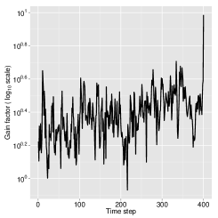
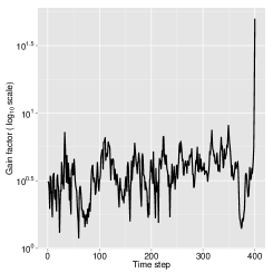
Full backward smoothing
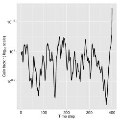
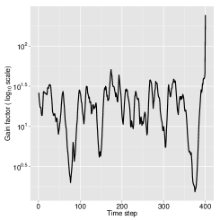
Marginal backward smoothing

Figure 2: Smoothing of the bivariate SV model (11) for $N=2^{8}$ and $N=2^{10}$ particles. The graphs give the gain factor (MSE ratio, from 100 replications) for comparing SQMC with SMC, and for $\mathbb{E}[x_{t1}|\mathbf{y}_{0:T}]$ as a function of $t$. The top line is for full backward smoothing (Algorithm 3), the bottom line is for marginal backward smoothing.

$N=2^{8}$	$N=2^{10}$

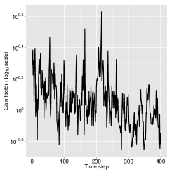
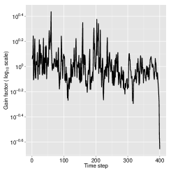
Figure 3: Smoothing of the bivariate SV model (11) for $N=2^{8}$ and $N=2^{10}$ particles. The graphs give the gain factor (MSE ratio, for 100 replications) of the hybrid backward pass (Algorithm 3 with IID input) relative to the QMC backward pass (Algorithm 3 with a QMC point set as input), for the estimation of $\mathbb{E}[x_{t1}|\mathbf{y}_{0:T}]$ as a function of $t$.

Figure 2 plots the gain factors at each time step, for either $N=2^{8}$ (left), or $N=2^{10}$ (right). We observe that gain factors tend to increase with $N$ (as expected) and that they are above one most of the time. They are not very high for full backward smoothing; but note that even a marginal improvement in terms of gain factor may translate in high CPU time savings, given that these algorithms have complexity $\mathcal{O}(N^{2})$; i.e. a gain factor of 3 means that SMC would need 3 times more particles, and therefore 9 times more CPU time, to reach the same accuracy as SQMC. Notice also gain factors are higher for marginal smoothing.

Finally, we compare Algorithm 3 (full backward smoothing) with the hybrid strategy described at the end of Section 5.3: i.e. a SQMC forward pass (Algorithm 2) followed by a Monte Carlo backward pass. Again, this is for $N=2^{8}$ (left) and $N=2^{10}$ (right). Interestingly, the hybrid strategy (slightly) dominates at most time steps (excepts those such that $T-t$ is small). As already discussed, the likely reason for this phenomenon is that the backward pass of Algorithm 3 is based on a point set of dimension $T$, which is too large to have good equidistribution properties (for reasonable values of $N$), and therefore to bring much improvement over plain Monte Carlo. Thus, for large $T$, one may as well use this hybrid strategy to perform full smoothing.

7 Conclusion

The estimation of the smoothing distribution $p(\mathbf{x}_{0:T}|\mathbf{y}_{0:T})$ is a challenging task for QMC methods because it is typically a high dimensional problem. On the other hand, due to the $\mathcal{O}(N^{2})$ complexity of most smoothing algorithms, small gains in term of mean square errors translate into important savings in term of running times to reach the same level of error. In this work we provide asymptotic results for some QMC smoothing strategies, namely forward smoothing, and two variants of forward-backward smoothing. In a simulation study we show that the QMC forward-backward smoothing algorithm outperforms its Monte Carlo counterpart despite of the high dimensional nature of the problem. Also, if one is interested in the estimation of the marginal smoothing distributions, more important gains may be obtained.

The set of smoothing strategies discussed in this work is obviously not exhaustive. For instance, we have not discussed two-filter smoothing (Briers et al.,, 2005), or its $\mathcal{O}(N)$ variant proposed by Fearnhead et al., (2010). In fact, our analysis can be easily applied to derive a QMC version of these algorithms and to provide conditions for their validity. An other interesting smoothing algorithm is proposed in Douc et al., (2011), where the backward pass is an accept-reject procedure, leading to a $\mathcal{O}(N)$ complexity. A last interesting smoothing strategy is the particle Gibbs sampler proposed by Andrieu et al., (2010) which generates a Markov chain having the smoothing distribution as stationary distribution. For these last two methods, the usefulness and the validity of replacing pseudo-random numbers by QMC point sets remain interesting open questions.

Appendix A Main properties of the Hilbert curve

Function $H$ is obtained as the limit of a certain sequence $(H_{m})$ of functions $H_{m}:[0,1]\rightarrow[0,1]^{d}$ as $m\rightarrow\infty$. The proofs of the results presented in this work are based on the following technical properties of $H$ and $H_{m}$. For $m\geq 0$, let $\mathcal{I}_{m}^{d}=\left\{I_{m}^{d}(k)\right\}_{k=0}^{2^{md}-1}$ be the collection of consecutive closed intervals in $[0,1]$ of equal size $2^{-md}$ and such that $\cup\mathcal{I}_{m}^{d}=[0,1]$. For $k\geq 0$, $S_{m}^{d}(k)=H_{m}(I_{m}^{d}(k))$ belongs to $\mathcal{S}_{m}^{d}$, the set of the $2^{md}$ closed hypercubes of volume $2^{-md}$ that covers $[0,1]^{d}$, $\cup\mathcal{S}_{m}^{d}=[0,1]^{d}$; $S_{m}^{d}(k)$ and $S_{m}^{d}(k+1)$ are adjacent, i.e. have at least one edge in common (adjacency property). If we split $I_{m}^{d}(k)$ into the $2^{d}$ successive closed intervals $I_{m+1}^{d}(k_{i})$, $k_{i}=2^{d}k+i$ and $i\in 0:2^{d}-1$, then the $S_{m+1}^{d}(k_{i})$’s are simply the splitting of $S_{m}^{d}(k)$ into $2^{d}$ closed hypercubes of volume $2^{-d(m+1)}$ (nesting property). Finally, the limit $H$ of $H_{m}$ has the bi-measure property: $\lambda_{1}(A)=\lambda_{d}(H(A))$, for any measurable set $A\subset[0,1]$, and satisfies the Hölder condition $\|H(x_{1})-H(x_{2})\|\leq C_{H}|x_{1}-x_{2}|^{1/d}$ for all $x_{1}$ and $x_{2}$ in $[0,1]$. For more background on space-filling curves, see Sagan, (1994).

Appendix B Proofs

B.1 Backward decomposition: Proof of Theorem 2

Lemma 2 of Gerber and Chopin, (2015) is central for the proof of this result and is reproduced here for sake of clarity.

Lemma 1.

Let $(\pi^{N})_{N\geq 1}$ be a sequence of probability measures on $[0,1)^{d_{1}}$ such that $\|\pi^{N}-\pi\|_{\mathrm{E}}\rightarrow 0$ as $N\rightarrow+\infty$ for some $\pi\in\mathcal{P}([0,1)^{d_{1}})$, and let $K$ a kernel $[0,1)^{d_{1}}\rightarrow\mathcal{P}([0,1)^{d_{2}}))$ such that $F_{K}(\mathbf{x}_{1},\mathbf{x}_{2})$ is Hölder continuous with its $i$-th component strictly increasing in $x_{2i}$, $i\in 1:d_{2}$. Then

$$\|\pi^{N}\otimes K-\pi\otimes K\|_{\mathrm{E}}={\scriptscriptstyle\mathcal{O}}(1).$$

From Theorem 1, we know that (for $t\geq 1$)

$$\|\mathcal{S}(P_{t,h}^{N})-\mathbb{Q}_{t-1,h}\otimes m_{t,h}\|_{\mathrm{E}}={\scriptscriptstyle\mathcal{O}}(1)\qquad\mbox{for }P_{t,h}^{N}=\left(h(\hat{\mathbf{x}}_{t-1}^{1:N}),\mathbf{x}_{t}^{1:N}\right).$$

To establish (6), we fix $\mathbf{x}_{t+1}$, and recognise $\mathcal{M}_{t+1,\mathbb{Q}_{t}}$ as the marginal distribution of $\mathbf{x}_{t}$, relative to joint distribution

$$\frac{\tilde{G}_{t+1}(\mathbf{x}_{t},\mathbf{x}_{t+1})G_{t,h}(h_{t-1},\mathbf{x}_{t})}{\mathbb{Q}_{t-1,h}\otimes m_{t,h}(G_{t,h})}\times\mathbb{Q}_{t-1,h}\otimes m_{t,h}\left(\mathrm{d}(h_{t-1},\mathbf{x}_{t})\right)$$ (12)

with $G_{t,h}(h_{t-1},\mathbf{x}_{t})=G_{t}(H(h_{t-1},\mathbf{x}_{t}))$. This is a change of measure applied to $\mathbb{Q}_{t-1,h}\otimes m_{t,h}$. Similarly, $\mathcal{M}_{t+1,\widehat{\mathbb{Q}}_{t}^{N}}$ is the marginal of a joint distribution obtained by the same change of measure, but applied to $\mathcal{S}(P_{t,h}^{N})$.

Thus, we may apply Theorem 1 of Gerber and Chopin, (2015), and deduce that (again for a fixed $\mathbf{x}_{t+1}$):

$$\|\mathcal{M}_{t+1,\widehat{\mathbb{Q}}^{N}_{t}}(\mathbf{x}_{t+1},\mathrm{d}\mathbf{x}_{t})-\mathcal{M}_{t+1,\mathbb{Q}_{t}}(\mathbf{x}_{t+1},\mathrm{d}\mathbf{x}_{t})\|_{\mathrm{E}}={\scriptscriptstyle\mathcal{O}}(1).$$

To see that the ${\scriptscriptstyle\mathcal{O}}(1)$ term in the above expression does not depend on $\mathbf{x}_{t+1}$, note that in (12), the dominating measure does not depends on $\mathbf{x}_{t+1}$, and the density with respect to this dominating measure is bounded uniformly with respect to $\mathbf{x}_{t+1}$, and therefore the results follows from the computations in the proof of Gerber and Chopin, (2015, Theorem 1). This shows (6) for $t\geq 1$. For $t=0$ replace $\mathbb{Q}_{t-1,h}\otimes m_{t,h}$ by $m_{0,h}$ in the above argument.

Let us now prove the second part of the theorem. As a preliminary result to establish (7) we show that, for all $t\geq 0$,

$$\|\widehat{\mathbb{Q}}_{t+1}^{N}\otimes\mathcal{M}_{t+1,\widehat{\mathbb{Q}}_{t}^{N}}-\mathbb{Q}_{t+1}\otimes\mathcal{M}_{t+1,\mathbb{Q}_{t}}\|_{\mathrm{E}}={\scriptscriptstyle\mathcal{O}}(1).$$ (13)

Let $B_{t}$ and $B_{t+1}$ be two sets in $\mathcal{B}_{[0,1)^{d}}$ and note $B_{t:t+1}=B_{t}\times B_{t+1}$ to simplify the notations. Then,

$$\left|\widehat{\mathbb{Q}}_{t+1}^{N}\otimes\mathcal{M}_{t+1,\widehat{\mathbb{Q}}_{t}^{N}}(B_{t:t+1})-\mathbb{Q}_{t+1}\otimes\mathcal{M}_{t+1,\mathbb{Q}_{t}}(B_{t:t+1})\right|$$

$$=\left|\int_{B_{t+1}}\lambda_{d}\left(F_{\mathcal{M}_{t+1,\widehat{\mathbb{Q}}_{t}^{N}}}(\mathbf{x}_{t+1},B_{t})\right)\widehat{\mathbb{Q}}_{t+1}^{N}(\mathrm{d}\mathbf{x}_{t+1})-\lambda_{d}\left(F_{\mathcal{M}_{t+1,\mathbb{Q}_{t}}}(\mathbf{x}_{t+1},B_{t})\right)\mathbb{Q}_{t+1}(\mathrm{d}\mathbf{x}_{t+1})\right|$$

$$\leq\left|\int_{B_{t+1}}\lambda_{d}\left(F_{\mathcal{M}_{t+1,\mathbb{Q}_{t}}}(\mathbf{x}_{t+1},B_{t})\right)\left(\widehat{\mathbb{Q}}_{t+1}^{N}-\mathbb{Q}_{t+1}\right)(\mathrm{d}\mathbf{x}_{t+1})\right|$$

$$+\left|\int_{B_{t+1}}\widehat{\mathbb{Q}}_{t+1}^{N}(\mathrm{d}\mathbf{x}_{t+1})\left[\lambda_{d}\left(F_{\mathcal{M}_{t+1,\widehat{\mathbb{Q}}_{t}^{N}}}(\mathbf{x}_{t+1},B_{t})\right)-\lambda_{d}\left(F_{\mathcal{M}_{t+1,\mathbb{Q}_{t}}}(\mathbf{x}_{t+1},B_{t})\right)\right]\right|.$$

By assumption, $F_{\mathcal{M}_{t+1,\mathbb{Q}_{t}}}(\mathbf{x}_{t+1},\mathbf{x}_{t})$ is Hölder continuous. Since $\|\widehat{\mathbb{Q}}_{t+1}^{N}-\mathbb{Q}_{t+1}\|_{\mathrm{E}}={\scriptscriptstyle\mathcal{O}}(1)$ by Theorem 1, Lemma 1 therefore implies

$$\sup_{B_{t:t+1}\in\mathcal{B}^{2}_{[0,1)^{d}}}\left|\int_{B_{t+1}}\lambda_{d}\left(F_{\mathcal{M}_{t+1,\mathbb{Q}_{t}}}(\mathbf{x}_{t+1},B_{t})\right)\left(\widehat{\mathbb{Q}}_{t+1}^{N}-\mathbb{Q}_{t+1}\right)(\mathrm{d}\mathbf{x}_{t+1})\right|={\scriptscriptstyle\mathcal{O}}(1).$$

In addition,

$$\left|\int_{B_{t+1}}\widehat{\mathbb{Q}}_{t+1}^{N}(\mathrm{d}\mathbf{x}_{t+1})\left[\lambda_{d}\left(F_{\mathcal{M}_{t+1,\widehat{\mathbb{Q}}_{t}^{N}}}(\mathbf{x}_{t+1},B_{t})\right)-\lambda_{d}\left(F_{\mathcal{M}_{t+1,\mathbb{Q}_{t}}}(\mathbf{x}_{t+1},B_{t})\right)\right]\right|$$

$$\leq\int_{B_{t+1}}\widehat{\mathbb{Q}}_{t+1}^{N}(\mathrm{d}\mathbf{x}_{t+1})\sup_{B_{t}\in\mathcal{B}_{[0,1)^{d}}}\left|\lambda_{d}\left(F_{\mathcal{M}_{t+1,\widehat{\mathbb{Q}}_{t}^{N}}}(\mathbf{x}_{t+1},B_{t})\right)-\lambda_{d}\left(F_{\mathcal{M}_{t+1,\mathbb{Q}_{t}}}(\mathbf{x}_{t+1},B_{t})\right)\right|$$

$$\leq\int_{B_{t+1}}\widehat{\mathbb{Q}}_{t+1}^{N}(\mathrm{d}\mathbf{x}_{t+1})\sup_{\mathbf{x}_{t+1}\in[0,1)^{d}}\|\mathcal{M}_{t+1,\widehat{\mathbb{Q}}_{t}^{N}}(\mathbf{x}_{t+1},\mathrm{d}\mathbf{x}_{t})-\mathcal{M}_{t+1,\mathbb{Q}_{t}}(\mathbf{x}_{t+1},\mathrm{d}\mathbf{x}_{t})\|_{\mathrm{E}}$$

$$={\scriptscriptstyle\mathcal{O}}(1)$$

using (6). This complete the proof of (13).

We are now ready to prove the second statement of the theorem. Note that (7) is true for $t=1$ by (13). Let $t>1$ and $B_{0:t}\in\mathcal{B}^{t+1}_{[0,1)^{d}}$. Then,

$$\left|\int_{B_{0:t}}\left(\widetilde{\mathbb{Q}}_{t}^{N}-\widetilde{\mathbb{Q}}_{t}\right)(\mathrm{d}\mathbf{x}_{0:t})\right|=\left|\int_{B_{0:t}}\left(\widehat{\mathbb{Q}}_{t}^{N}\otimes\mathcal{M}_{t,\widehat{\mathbb{Q}}^{N}_{t-1}}(\mathrm{d}\mathbf{x}_{t-1:t})\prod_{s=1}^{t-1}\mathcal{M}_{s,\widehat{\mathbb{Q}}_{s-1}^{N}}(\mathbf{x}_{s},\mathrm{d}\mathbf{x}_{s-1})\right.\right.$$

$$-\left.\left.\mathbb{Q}_{t}\otimes\mathcal{M}_{t,\mathbb{Q}_{t-1}}(\mathrm{d}\mathbf{x}_{t-1:t})\prod_{s=1}^{t-1}\mathcal{M}_{s,\mathbb{Q}_{s-1}}(\mathbf{x}_{s},\mathrm{d}\mathbf{x}_{s-1})\right)\right|$$

$$\leq\left|\int_{B_{t-1:t}}\left[\int_{B_{0:t-2}}\prod_{s=1}^{t-1}\mathcal{M}_{s,\mathbb{Q}_{s-1}}(\mathbf{x}_{s},\mathrm{d}\mathbf{x}_{s-1})\right]\left(\widehat{\mathbb{Q}}_{t}^{N}\otimes\mathcal{M}_{t,\widehat{\mathbb{Q}}_{t-1}^{N}}-\mathbb{Q}_{t}\otimes\mathcal{M}_{t,\mathbb{Q}_{t-1}}\right)(\mathrm{d}\mathbf{x}_{t-1:t})\right|$$

$$+\left|\int_{B_{t-1:t}}\widehat{\mathbb{Q}}_{t}^{N}\otimes\mathcal{M}_{t,\widehat{\mathbb{Q}}_{t-1}^{N}}(\mathrm{d}\mathbf{x}_{t-1:t})\left(\int_{B_{0:t-2}}\prod_{s=1}^{t-1}\mathcal{M}_{s,\widehat{\mathbb{Q}}^{N}_{s-1}}(\mathbf{x}_{s},\mathrm{d}\mathbf{x}_{s-1})-\int_{B_{0:t-2}}\prod_{s=1}^{t-1}\mathcal{M}_{s,\mathbb{Q}_{s-1}}(\mathbf{x}_{s},\mathrm{d}\mathbf{x}_{s-1})\right)\right|.$$

The first term after the inequality sign can be rewritten as

$$\left|\int_{B_{t-1:t}}\lambda_{(t-1)d}\left(F_{\otimes_{s=1}^{t-1}\mathcal{M}_{s,\mathbb{Q}_{s-1}}}(\mathbf{x}_{t-1},B_{0:t-2})\right)\left(\widehat{\mathbb{Q}}_{t}^{N}\otimes\mathcal{M}_{t,\widehat{\mathbb{Q}}_{t-1}^{N}}-\mathbb{Q}_{t}\otimes\mathcal{M}_{t,\mathbb{Q}_{t-1}}\right)(\mathrm{d}\mathbf{x}_{t-1:t})\right|.$$

The supremum of this quantity over $B_{0:t}\in\mathcal{B}^{t+1}_{[0,1)^{d}}$ is ${\scriptscriptstyle\mathcal{O}}(1)$ using (13), the fact that $F_{\otimes_{s=1}^{t-1}\mathcal{M}_{s,\mathbb{Q}_{s-1}}}$ is Hölder continuous (because $F_{\mathcal{M}_{s,\mathbb{Q}_{s-1}}}$ is Hölder continuous for all $s$) and Lemma 1.

To control the second term we first prove by induction that, for any $t>1$,

$$\sup_{B_{0:t-2}\in\mathcal{B}^{t-1}_{[0,1)^{d}}}\left|\int_{B_{0:t-2}}\prod_{s=1}^{t-1}\mathcal{M}_{s,\widehat{\mathbb{Q}}^{N}_{s-1}}(\mathbf{x}_{s},\mathrm{d}\mathbf{x}_{s-1})-\int_{B_{0:t-2}}\prod_{s=1}^{t-1}\mathcal{M}_{s,\mathbb{Q}_{s-1}}(\mathbf{x}_{s},\mathrm{d}\mathbf{x}_{s-1})\right|={\scriptscriptstyle\mathcal{O}}(1)$$ (14)

uniformly on $\mathbf{x}_{t-1}$. By (6) this result is true for $t=2$. Assume that (14) holds for $t>2$. Then

$$\left|\int_{B_{0:t-1}}\prod_{s=1}^{t}\mathcal{M}_{s,\widehat{\mathbb{Q}}^{N}_{s-1}}(\mathbf{x}_{s},\mathrm{d}\mathbf{x}_{s-1})-\int_{B_{0:t-1}}\prod_{s=1}^{t}\mathcal{M}_{s,\mathbb{Q}_{s-1}}(\mathbf{x}_{s},\mathrm{d}\mathbf{x}_{s-1})\right|$$

$$=\left|\int_{B_{0:t-1}}\left[\mathcal{M}_{t,\widehat{\mathbb{Q}}^{N}_{t-1}}(\mathbf{x}_{t},\mathrm{d}\mathbf{x}_{t-1})\prod_{s=1}^{t-1}\mathcal{M}_{s,\widehat{\mathbb{Q}}^{N}_{s-1}}(\mathbf{x}_{s},\mathrm{d}\mathbf{x}_{s-1})\right.\right.$$

$$-\left.\left.\mathcal{M}_{t,\mathbb{Q}_{t-1}}(\mathbf{x}_{t},\mathrm{d}\mathbf{x}_{t-1})\prod_{s=1}^{t-1}\mathcal{M}_{s,\mathbb{Q}_{s-1}}(\mathbf{x}_{s},\mathrm{d}\mathbf{x}_{s-1})\right]\right|$$

$$\leq\left|\int_{B_{t-1}}\mathcal{M}_{t,\widehat{\mathbb{Q}}^{N}_{t-1}}(\mathbf{x}_{t},\mathrm{d}\mathbf{x}_{t-1})\int_{B_{0:t-2}}\left(\prod_{s=1}^{t-1}\mathcal{M}_{s,\widehat{\mathbb{Q}}^{N}_{s-1}}(\mathbf{x}_{s},\mathrm{d}\mathbf{x}_{s-1})-\prod_{s=1}^{t-1}\mathcal{M}_{s,\mathbb{Q}_{s-1}}(\mathbf{x}_{s},\mathrm{d}\mathbf{x}_{s-1})\right)\right|$$

$$+\left|\int_{B_{t-1}}\lambda_{(t-1)d}\left(F_{\otimes_{s=1}^{t-1}\mathcal{M}_{s,\mathbb{Q}_{s-1}}}(\mathbf{x}_{t-1},B_{0:t-2})\right)\left(\mathcal{M}_{t,\widehat{\mathbb{Q}}^{N}_{t-1}}(\mathbf{x}_{t},\mathrm{d}\mathbf{x}_{t-1})-\mathcal{M}_{t,\mathbb{Q}_{t-1}}(\mathbf{x}_{t},\mathrm{d}\mathbf{x}_{t-1})\right)\right|$$

where we saw above that second term on the right side of the inequality sign is ${\scriptscriptstyle\mathcal{O}}(1)$ uniformly on $\mathbf{x}_{t}$ while the first term is bounded by

$$\int_{[0,1)^{d}}\mathcal{M}_{t,\widehat{\mathbb{Q}}^{N}_{t-1}}(\mathbf{x}_{t},\mathrm{d}\mathbf{x}_{t-1})$$

$$\times\sup_{B_{0:t-2}\in\mathcal{B}^{t-1}_{[0,1)^{d}}}\left|\int_{B_{0:t-2}}\left(\prod_{s=1}^{t-1}\mathcal{M}_{s,\widehat{\mathbb{Q}}^{N}_{s-1}}(\mathbf{x}_{s},\mathrm{d}\mathbf{x}_{s-1})-\prod_{s=1}^{t-1}\mathcal{M}_{s,\mathbb{Q}_{s-1}}(\mathbf{x}_{s},\mathrm{d}\mathbf{x}_{s-1})\right)\right|$$

where, by the inductive hypothesis, the second factor is ${\scriptscriptstyle\mathcal{O}}(1)$ uniformly on $\mathbf{x}_{t-1}\in[0,1)^{d}$. This shows that (14) is true at time $t+1$ and therefore the proof of the theorem is complete.

B.2 Generalization of Hlawka and Mück, (1972): Proof of Theorem 3

The proof of this result is an adaptation of the proof of Hlawka and Mück, (1972, “Satz 2”).

In what follows, we use the shorthand $\alpha_{N}(B)=\mathcal{S}(\mathbf{u}^{1:N})(B)=N^{-1}\sum_{n=1}^{N}\mathds{1}_{B}(u^{n})$ for any set $B\subset[0,1)^{d}$. One has

$$\|\mathcal{S}(\mathbf{x}^{1:N})-\pi\|_{\mathrm{E}}=\sup_{B\in\mathcal{B}_{[0,1)^{d}}}\left|\alpha_{N}\left(F_{\pi}(B)\right)-\lambda_{d}\left(F_{\pi}(B)\right)\right|.$$

Let $\beta=\lceil\kappa^{-1}\rceil$, $\tilde{d}=\sum_{i=0}^{d-1}\beta^{i}$, $L$ an arbitrary integer, and $\mathcal{P}$ be the partition of $[0,1)^{d}$ in $L^{\tilde{d}}$ congruent hyperrectangles $W$ of size $L^{-\beta^{d-1}}\times L^{-\beta^{d-2}}\times...\times L^{-1}$. Let $B\in\mathcal{B}_{[0,1)^{d}}$, $\mathcal{U}_{1}$ the set of the elements of $\mathcal{P}$ that are strictly in $F_{\pi}(B)$, $\mathcal{U}_{2}$ the set of elements $W\in\mathcal{P}$ such that $W\cap\partial(F_{\pi}(B))\neq\varnothing$, $U_{1}=\cup\text{ }\mathcal{U}_{1}$, $U_{2}=\cup\text{ }\mathcal{U}_{2}$, and $U_{1}^{\prime}=F_{\pi}(B)\setminus U_{1}$ so that (Hlawka and Mück,, 1972, “Satz 2” or Gerber and Chopin,, 2015, Theorem 4)

$$\left|\alpha_{N}\left(F_{\pi}(B)\right)-\lambda_{d}\left(F_{\pi}(B)\right)\right| \leq|\alpha_{N}(U_{1})-\lambda_{d}(U_{1})|+\#\mathcal{U}_{2}\left\{D(\mathbf{u}^{1:N})+L^{-\tilde{d}}\right\}$$

where, under the assumption of the theorem, $|\alpha_{N}(U_{1})-\lambda_{d}(U_{1})|\leq L^{\tilde{d}-1}D(\mathbf{u}^{1:N})$ (see Hlawka and Mück,, 1972).

To bound $\#\mathcal{U}_{2}$, we first construct a partition $\mathcal{P}^{\prime}$ of $[0,1)^{d}$ into hyperrectangles $W^{\prime}$ of size $L^{\prime}{}^{-\beta^{d-1}}\times...\times L^{\prime}{}^{-1}$ such that, for all points $\mathbf{x}$ and $\mathbf{x}^{\prime}$ in $W^{\prime}$, we have

$$|F_{i}(x_{1:i-1},x_{i})-F_{i}(x^{\prime}_{1:i-1},x^{\prime}_{i})|\leq L^{-\beta^{d-i}},\quad i=1,...,d$$ (15)

where $F_{i}(x_{1:i-1},x_{i})$ denotes the $i$-th component of $F_{\pi}(\mathbf{x})$ (with $F_{i}(x_{1:i-1},x_{i})=F_{1}(x_{1})$ when $i=1$). To that effect, let $i\in 2:d$ and note that

$$|F_{i}(x_{1:i-1},x_{i})-F_{i}(x^{\prime}_{1:i-1},x^{\prime}_{i})|\leq|F_{i}(x_{1:i-1},x_{i})-F_{i}(x_{1:i-1},x^{\prime}_{i})|\\ +|F_{i}(x_{1:i-1},x^{\prime}_{i})-F_{i}(x^{\prime}_{1:i-1},x^{\prime}_{i})|.$$

By Assumption 3, the probability measure $\pi_{i}(x_{1:i-1},\mathrm{d}x_{i})$ admits a density $p_{i}(x_{i}|x_{1:i-1})$ with respect to the Lebesgue measure such that $\|p_{i}(\cdot|\cdot)\|_{\infty}<+\infty$. Therefore, the first term after the inequality sign is bounded by $\|p_{i}\|_{\infty}L^{\prime}{}^{-\beta^{d-i}}$. For the second term, the Hölder property of $F_{\pi}$ implies that

$$|F_{i}(x_{1:i-1},x^{\prime}_{i})-F_{i}(x^{\prime}_{1:i-1},x^{\prime}_{i})| \leq C_{\pi}(i-1)^{\kappa/2}(L^{\prime}{}^{-\beta^{d+1-i}})^{\kappa}$$

$$\leq C_{\pi}(i-1)^{\kappa/2}(L^{\prime}{}^{-\beta^{d+1-i}})^{1/\beta}=C_{\pi}(i-1)^{\kappa/2}L^{\prime}{}^{-\beta^{d-i}}$$

with $C_{\pi}$ the Hölder constant of $F_{\pi}$. For $i=1$, we simply have

$$|F_{1}(x_{1})-F_{1}(x_{1}^{\prime})|\leq\|p_{1}\|_{\infty}L^{\prime}{}^{-\beta^{d-1}}.$$

Condition (15) is therefore verified for $L^{\prime}$ the smallest integer such that $L^{\prime}\geq\tilde{C}L$, for some $\tilde{C}>0$.

Remark now that $\partial(F_{\pi}(B))=F_{\pi}(\partial(B))$ since $F$ is a continuous function. Let $R\in\partial B$ be a $(d-1)$-dimensional face of $B$ and $\mathcal{R}$ be the set of hyper-rectangles $W^{\prime}\in\mathcal{P}^{\prime}$ such that $R\cap W^{\prime}\neq\varnothing$. Note that $\#\mathcal{R}\leq L^{\prime}{}^{\tilde{d}-1}\leq(\lfloor\tilde{C}L\rfloor+1)^{\tilde{d}-1}$. For each $W^{\prime}\in\mathcal{R}$, take a point $\mathbf{r}^{W^{\prime}}\in R\cap W^{\prime}$ and define

$$\tilde{\mathbf{r}}^{W^{\prime}}=F_{\pi}(\mathbf{r}^{W^{\prime}})\in F_{\pi}(R).$$

Let $\tilde{\mathcal{R}}$ be the collection of hyper-rectangles $\tilde{W}$ of size $2L^{-\beta^{d-1}}\times...\times 2L^{-1}$ (assuming $L$ is even) and having point $\tilde{\mathbf{r}}^{W^{\prime}}$, $W^{\prime}\in\mathcal{R}$, as a middle point.

For an arbitrary $\mathbf{u}\in F_{\pi}(R)$, let $\mathbf{x}=F^{-1}_{\pi}(\mathbf{u})\in R$. Hence, $\mathbf{x}$ is in one hyperrectangle $W^{\prime}\in\mathcal{R}$ so that using (15)

$$|u_{i}-\tilde{r}_{i}^{W^{\prime}}|=|F_{i}(x_{1:i-1},x_{i})-F_{i}(r_{1:i-1}^{W^{\prime}},r_{i}^{W^{\prime}})|\leq L^{-\beta^{d-i}},\quad i=1,\dots,d.$$

This shows that $\mathbf{u}$ belongs to the hyperrectangle $\tilde{W}\in\tilde{\mathcal{R}}$ with centre $\tilde{\mathbf{r}}^{W^{\prime}}$ so that $F_{\pi}(R)$ is covered by at most $\#\tilde{\mathcal{R}}=\#\mathcal{R}\leq(\lfloor\tilde{C}L\rfloor+1)^{\tilde{d}-1}$ hyperrectangles $\tilde{W}\in\tilde{\mathcal{R}}$. To go back to the initial partition of $[0,1)^{d}$ with hyperrectangles in $\mathcal{P}$, remark that every hyperrectangle in $\tilde{\mathcal{R}}$ is covered by at most $c_{1}$ hyperrectangles in $\mathcal{P}$ for a constant $c_{1}$. Finally, since the set $\partial B$ is made of the union of $2d$ $(d-1)$-dimensional faces of $B$, we have $\#\mathcal{U}_{2}\leq c_{2}L^{\tilde{d}-1}$ for a constant $c_{2}$.

Then, we may conclude the proof as follows

$$\|\mathcal{S}(\mathbf{x}^{1:N})-\pi\|_{\mathrm{E}} \leq L^{\tilde{d}-1}D(\mathbf{u}^{1:N})+c_{2}L^{\tilde{d}-1}\left(D(\mathbf{u}^{1:N})+L^{-\tilde{d}}\right)$$

where the optimal value of $L$ is such that, for some $c_{3}>0$,

$$\|\mathcal{S}(\mathbf{x}^{1:N})-\pi\|_{\mathrm{E}}\leq c_{3}D(\mathbf{u}^{1:N})^{1/\tilde{d}}.$$

B.3 Consistency of forward smoothing: Proof of Proposition 1

The proof amounts to a simple adaptation of Theorem 1: by replacing Assumption 4 by Assumption 4’ above, one obtains that $\|\mathcal{S}(\tilde{P}^{N}_{t,h^{t}})-\widetilde{\mathbb{Q}}_{t-1,h^{t}}\otimes m_{t,h}\|_{\mathrm{E}}\rightarrow 0$ as $N\rightarrow+\infty$, where $\tilde{P}^{N}_{t,h^{t}}=\left(h^{t}(\hat{\mathbf{z}}^{1:N}_{t-1}),\mathbf{x}_{t}^{1:N}\right)$ $\widetilde{\mathbb{Q}}_{t-1,h^{t}}$ is the image by $h^{t}$ of $\widetilde{\mathbb{Q}}_{t-1}$, and $m_{t,h}$ is defined as in Theorem 1. Therefore, by Corollary 1,

$$\|\mathcal{S}(\mathbf{z}_{t}^{1:N})-\widetilde{\mathbb{Q}}_{t-1}\otimes m_{t}\|_{\mathrm{E}}\rightarrow 0,\quad\mbox{as }N\rightarrow+\infty.$$ (16)

In addition, since the Radon-Nikodym derivative

$$\frac{\widetilde{\mathbb{Q}}_{t}}{\widetilde{\mathbb{Q}}_{t-1}\otimes m_{t}}\left(\mathrm{d}(\mathbf{x}_{0:t-1},\mathbf{x}_{t})\right)\propto G_{t}(\mathbf{x}_{t-1},\mathbf{x}_{t-1}),$$

is continuous and bounded, Theorem 1 of Gerber and Chopin, (2015), together with (16), implies (9).

B.4 $L_{2}$-convergence: Proof of Theorem 5

To prove the result, let $\varphi$ be as in the statement of the theorem and let us first prove the $L_{1}$-convergence.

We have

$$\mathbb{E}\left|\mathcal{S}(\tilde{\mathbf{x}}_{0:T}^{1:N})(\varphi)-\widetilde{\mathbb{Q}}_{T}(\varphi)\right|\leq\mathbb{E}\left|\mathcal{S}(\tilde{\mathbf{x}}_{0:T}^{1:N})(\varphi)-\widetilde{\mathbb{Q}}^{N}_{T}(\varphi)\right|+\mathbb{E}\left|\widetilde{\mathbb{Q}}^{N}_{T}(\varphi)-\widetilde{\mathbb{Q}}_{T}(\varphi)\right|.$$

By portmanteau lemma (Van der Vaart,, 2007, Lemma 2.2, p.6), convergence in the sense of the extreme metric is stronger than weak convergence. Hence, the second term above goes to 0 as $N\rightarrow+\infty$ by Theorem 2 and by the dominated convergence theorem. For the first term, as each $\tilde{\mathbf{u}}^{n}\sim\mathcal{U}([0,1)^{T+1})$, we have, by the inverse Rosenblatt interpretation of the backward pass of SQMC,

$$\mathbb{E}\Big{[}\mathcal{S}(\tilde{\mathbf{x}}_{0:T}^{1:N})(\varphi)\big{|}\mathcal{F}_{T}\Big{]}=\mathbb{E}\Big{[}\mathcal{S}(\tilde{h}_{0:T}^{1:N})(\varphi\circ H_{T})\big{|}\mathcal{F}_{T}\Big{]}=\widetilde{\mathbb{Q}}^{N}_{T,h_{T}}(\varphi\circ H_{T})=\widetilde{\mathbb{Q}}^{N}_{T}(\varphi)$$

with $\mathcal{F}_{T}^{N}$ the $\sigma$-algebra generated by the forward step (Algorithm 2). Therefore,

$$\mathbb{E}\left[\big{|}\mathcal{S}(\tilde{\mathbf{x}}_{0:T}^{1:N})(\varphi)-\widetilde{\mathbb{Q}}^{N}_{T}(\varphi)\big{|}\,\big{|}\mathcal{F}_{T}\right]\leq\mathrm{Var}\Big{(}\mathcal{S}(\tilde{\mathbf{x}}_{0:T}^{1:N})(\varphi)\big{|}\mathcal{F}_{T}\Big{)}^{1/2}$$ (17)

where, using Assumption 2 and the fact that $\tilde{\mathbf{x}}^{n}_{0:T}=H_{T}\circ F^{-1}_{\widetilde{\mathbb{Q}}^{N}_{T,h_{T}}}(\tilde{\mathbf{u}}^{n})$,

$$\mathrm{Var}\Big{(}\mathcal{S}(\tilde{\mathbf{x}}_{0:T}^{1:N})(\varphi)|\mathcal{F}^{N}_{T})\Big{)}\leq Cr(N)\sigma_{\varphi,N}^{2}$$ (18)

with $\sigma_{\varphi,N}^{2}\leq\widetilde{\mathbb{Q}}_{T}^{N}(\varphi^{2})$ and with $C$ and $r(N)$ as in the statement of the theorem. Let $\epsilon>0$. Then, by Assumption 1 and looking at the proof of Theorem 2, we have for $N$ large enough and almost surely, $\widetilde{\mathbb{Q}}_{T}^{N}(\varphi^{2})\leq\widetilde{\mathbb{Q}}_{T}(\varphi^{2})+\epsilon$ so that, for $N$ large enough,

$$\mathbb{E}\left|\mathcal{S}(\tilde{\mathbf{x}}_{0:T}^{1:N})(\varphi)-\widetilde{\mathbb{Q}}^{N}_{T}(\varphi)\right|\leq\sqrt{Cr(N)\big{(}\widetilde{\mathbb{Q}}_{T}(\varphi^{2})+\epsilon\big{)}}$$ (19)

showing the $L_{1}$-convergence. To prove the $L_{2}$-convergence, remark that

$$\mathbb{E}\left[\mathcal{S}(\tilde{\mathbf{x}}_{0:T}^{1:N})(\varphi)|\mathcal{F}^{N}_{T}\right]=\widetilde{\mathbb{Q}}_{T}^{N}(\varphi)=\big{(}\widetilde{\mathbb{Q}}^{N}_{T}(\varphi)-\widetilde{\mathbb{Q}}_{T}(\varphi)\big{)}+\widetilde{\mathbb{Q}}_{T}(\varphi)$$

and therefore

$$\mathrm{Var}\Big{(}\mathbb{E}\Big{[}\mathcal{S}(\tilde{\mathbf{x}}_{0:T}^{1:N})(\varphi)|\mathcal{F}^{N}_{T}\Big{]}\Big{)}=\mathrm{Var}\Big{(}\widetilde{\mathbb{Q}}^{N}_{T}(\varphi)-\widetilde{\mathbb{Q}}_{T}(\varphi)\Big{)}\leq\mathbb{E}\Big{[}\big{(}\widetilde{\mathbb{Q}}^{N}_{T}(\varphi)-\widetilde{\mathbb{Q}}_{T}(\varphi)\big{)}^{2}\Big{]}$$

where the right-hand side converges to zero as $N\rightarrow+\infty$ by the dominated convergence theorem and by Theorem 2. On conclude the prove using (17)-(19) and the fact that

$$\mathrm{Var}\Big{(}\mathcal{S}(\tilde{\mathbf{x}}_{0:T}^{1:N})(\varphi)\Big{)} =\mathrm{Var}\Big{(}\mathbb{E}\Big{[}\mathcal{S}(\tilde{\mathbf{x}}_{0:T}^{1:N})(\varphi)|\mathcal{F}^{N}_{T}\Big{]}\Big{)}+\mathbb{E}\Big{[}\mathrm{Var}\Big{(}\mathcal{S}(\tilde{\mathbf{x}}_{0:T}^{1:N})(\varphi)|\mathcal{F}^{N}_{T}\Big{)}\Big{]}.$$

B.5 Consistency of the Backward step: Proof of Theorem 6 and proof of Corollary 2

B.5.1 Preliminary computations

To prove Theorem 6 we need the following two lemmas:

Lemma 2.

Let $m\in\mathbb{N}$, $I=[0,\frac{k+1}{2^{dm}}]$, $k\in\{0,1,...,2^{dm}-2\}$ and $B=H(I)$. Then, $B=\cup_{i=1}^{p}B_{i}$ for some closed hyperrectangles $B_{i}\subseteq[0,1]^{d}$ and where $p\leq 2^{d}(m+1)$.

Proof.

To prove the Lemma, let $0\leq m_{1}\leq m$ be the smallest integer $\tilde{m}$ such that $I^{d}_{\tilde{m}}(0)\subseteq I$ and $i^{*}_{m_{1}}$ be the number of intervals in $\mathcal{I}^{d}_{m_{1}}$ included in $I$. Note that $i^{*}_{m_{1}}<2^{d}$. Indeed, if $i^{*}_{m_{1}}\geq 2^{d}$ then, by the nesting property of the Hilbert curve,

$$I^{d}_{m_{1}-1}(0)\subseteq\bigcup_{k=0}^{2^{d}-1}I^{d}_{m_{1}}(k)\subseteq\bigcup_{k=0}^{i^{*}_{m_{1}}-1}I^{d}_{m_{1}}(k)\subseteq I$$

which is in contradiction with the definition of $i^{*}_{m_{1}}$. Define $I_{2}=I\setminus\cup\mathcal{I}^{I}_{m_{1}}$ and $i^{*}_{m_{2}}$ the number of intervals in $\mathcal{I}^{d}_{m_{2}}$ included in $I_{2}$. For the same reason as above $i^{*}_{n_{2}}<2^{d}$. More generally, for any $m_{1}\leq m_{k}\leq m$, $i^{*}_{m_{k}}\leq 2^{d}$ meaning that the set $B$ is made of at most $\sum_{k=m_{1}}^{m}i^{*}_{m_{k}}\leq 2^{d}(m+1)$ hypercubes (of side varying between $2^{-m}$ and $2^{-m_{1}}$). ∎

Lemma 3.

Let $(\pi^{N})_{N\geq 1}$ be a sequence of probability measures on $[0,1)^{(k+1)d}$ such that $\|\pi^{N}-\pi\|_{\mathrm{E}}\rightarrow 0$ where $\pi(\mathrm{d}\mathbf{x})=\pi(\mathbf{x})\lambda_{(k+1)d}(\mathrm{d}\mathbf{x})$ is a probability measure on $\pi^{(k+1)d}$ that admits a bounded density $\pi(\mathbf{x})$. Let $\pi_{h_{k}}$ be the image by $h_{k}$ of $\pi$. Then,

$$\|\pi_{h_{k}}^{N}-\pi_{h_{k}}\|_{\mathrm{E}}\rightarrow 0,\quad\mbox{as }N\rightarrow+\infty.$$

The proof of this last result is omitted since it follows from the properties of Cartesian products and from straightforward modifications of the proof of Gerber and Chopin, (2015, Theorem 3).

B.5.2 Proof of the Theorem 6

To prove the theorem first note that

$$\|\widetilde{\mathsf{Q}}_{T,h_{T}}^{N}-\widetilde{\mathbb{Q}}_{T,h_{T}}\|_{\mathrm{E}}={\scriptscriptstyle\mathcal{O}}(1).$$

Indeed, by assumption, $\|\widehat{\mathsf{Q}}_{T,h}^{N}-\widehat{\mathbb{Q}}_{T,h}^{N}\|_{\mathrm{E}}={\scriptscriptstyle\mathcal{O}}(1)$ and, by Theorem 1 and Gerber and Chopin, (2015, Theorem 3), $\|\widehat{\mathbb{Q}}_{T,h}^{N}-\mathbb{Q}_{T,h}\|_{\mathrm{E}}={\scriptscriptstyle\mathcal{O}}(1)$ since $\mathbb{Q}_{T}$ admits a bounded density (Assumption 4 of Theorem 1). Hence, $\|\widehat{\mathsf{Q}}_{T,h}^{N}-\mathbb{Q}_{T,h}\|_{\mathrm{E}}={\scriptscriptstyle\mathcal{O}}(1)$ and thus, by Theorem 4, $\|\widehat{\mathsf{Q}}_{T}^{N}-\mathbb{Q}_{T}\|_{\mathrm{E}}={\scriptscriptstyle\mathcal{O}}(1)$, with $\widehat{\mathsf{Q}}_{T}^{N}$ the image by $H$ of $\widehat{\mathsf{Q}}_{T,h}^{N}$. In addition, using the same argument, and using the fact that, for all $t\in 1:T$, $\tilde{G}_{t}$ is bounded (Assumption H1 of Theorem 2), we have, by Theorem 2 (first part),

$$\sup_{\mathbf{x}_{t}\in\mathcal{X}}\|K^{N}_{t}(\mathbf{x}_{t},\mathrm{d}\mathbf{x}_{t-1})-\mathcal{M}_{t,\mathbb{Q}_{t-1}}(\mathbf{x}_{t},\mathrm{d}\mathbf{x}_{t-1})\|_{\mathrm{E}}={\scriptscriptstyle\mathcal{O}}(1),\quad t\in 1:T$$

with $K^{N}_{t}(\mathbf{x}_{t},\mathrm{d}\mathbf{x}_{t-1})$ the image by $H$ of the probability measure $K_{t,h}(H(\mathbf{x}_{t}),\mathrm{d}h_{t-1})$. Consequently, by the second part of Theorem 2, $\|\widetilde{\mathsf{Q}}_{T}^{N}-\widetilde{\mathbb{Q}}_{T}\|_{\mathrm{E}}={\scriptscriptstyle\mathcal{O}}(1)$ where $\widetilde{\mathsf{Q}}_{T}^{N}$ denotes the image by $H_{T}$ of $\widetilde{\mathsf{Q}}_{T,h_{T}}^{N}$. Finally, under the assumptions of the theorem, $\widetilde{\mathbb{Q}}_{T}$ admits a bounded density (because for all $t$, $\tilde{G}_{t}$ is bounded and $\mathbb{Q}_{t}$ admits a bounded density) and thus, by Lemma 3, $\|\widetilde{\mathsf{Q}}_{T,h_{T}}^{N}-\widetilde{\mathbb{Q}}_{T,h_{T}}\|_{\mathrm{E}}={\scriptscriptstyle\mathcal{O}}(1)$.

To prove the theorem it therefore remains to show that

$$\|\mathcal{S}(\check{h}_{0:T}^{1:N})-\widetilde{\mathsf{Q}}_{T,h_{T}}^{N}\|_{\mathrm{E}}={\scriptscriptstyle\mathcal{O}}(1).$$ (20)

Indeed, this would yield $\|\mathcal{S}(\check{h}_{0:T}^{1:N})-\widetilde{\mathbb{Q}}_{T,h_{T}}\|_{\mathrm{E}}={\scriptscriptstyle\mathcal{O}}(1)$ and thus, by Theorem 4,

$$\|\mathcal{S}(\check{\mathbf{x}}_{0:T}^{1:N})-\widetilde{\mathbb{Q}}_{T}\|_{\mathrm{E}}={\scriptscriptstyle\mathcal{O}}(1)$$

as required.

To prove (20), we assume to simplify the notations that $F_{\mathcal{M}_{t,\mathbb{Q}_{t-1}}}(\mathbf{x}_{t},\mathbf{x}_{t-1})$ is Lipschitz. Generalization for any Hölder exponent can be done using similar arguments as in the proof of Theorem 3.

Let $h_{t}^{n}=h(\mathbf{x}_{t}^{N})$ where $\mathbf{x}_{t}^{1:N}$ are the particles obtained at the end of iteration $t$ of Algorithm 2. We assume that, for all $t\in 0:T$, the particles are sorted according to their Hilbert index, i.e. $n<m\implies h_{t}^{n}<h_{t}^{m}$ (note that the inequality is strict by Assumption 1 of Theorem 1). Then, using the same notation as in the proof of Theorem 3, one has

$$\|\mathcal{S}(\check{h}_{0:T}^{1:N})-\widetilde{\mathsf{Q}}_{T,h_{T}}^{N}\|_{\mathrm{E}}=\sup_{B\in\mathcal{B}^{N}_{[0,1)^{T+1}}}\left|\alpha_{N}\left(F_{\widetilde{\mathsf{Q}}_{T,h_{T}}^{N}}(B)\right)-\lambda_{T+1}\left(F_{\widetilde{\mathsf{Q}}_{T,h_{T}}^{N}}(B)\right)\right|$$

where $\mathcal{B}^{N}_{[0,1)^{T+1}}=\left\{[\bm{a},\bm{b}]\subset\mathcal{B}_{[0,1)^{T+1}},\,b_{i}^{N}\leq h_{i}^{N},\,i\in 0:T\right\}$.

The beginning of the proof follows the lines of Theorem 3, with $\beta=d$ and $d$ replaced by $T+1$. Let $\tilde{d}=\sum_{t=0}^{T}d^{t}$ so that, for a set $B\in\mathcal{B}^{N}_{[0,1)^{T+1}}$,

$$\left|\alpha_{N}\left(F_{\widetilde{\mathsf{Q}}_{T,h_{T}}^{N}}(B)\right)-\lambda_{T+1}\left(F_{\widetilde{\mathsf{Q}}_{T,h_{T}}^{N}}(B)\right)\right|\leq L^{\tilde{d}}D(\mathbf{u}^{1:N})+\#\mathcal{U}_{2}\left\{D(\mathbf{u}^{1:N})+L^{-\tilde{d}}\right\}$$

where $L$ and $\mathcal{U}_{2}$ are as in the proof of Theorem 3.

Following this latter, let $\mathcal{P}^{\prime}$ be the partition of the set $[0,1)^{T+1}$ into hyperrectangles $W^{\prime}$ of size $L^{\prime}{}^{-d^{T}}\times L^{\prime}{}^{-d^{T-1}}\times...\times L^{\prime}{}^{-1}$ such that, for all $\bm{h}$ and $\bm{h}^{\prime}$ in $W^{\prime}$, we have

$$|F_{\widehat{\mathsf{Q}}_{T,h}^{N}}(h_{t})-F_{\widehat{\mathsf{Q}}_{T,h}^{N}}(h_{1}^{\prime})|\leq L^{-d^{T}}.$$ (21)

and

$$\left|\tilde{F}^{N}_{i-1}(h_{i-1},h_{i})-\tilde{F}^{N}_{i-1}(h^{\prime}_{i-1},h^{\prime}_{i})\right|\leq L^{-d^{T+1-i}},\quad i\in 2:(T+1)$$ (22)

where, to simplify the notation, we write $\tilde{F}^{N}_{i-1}(\tilde{h},\cdot)$ the CDF of $K^{N}_{T-i+2,h}(\tilde{h},\mathrm{d}h_{T-i+1})$.

Let us first look at condition (21). We have

$$|F_{\widehat{\mathsf{Q}}_{T,h}^{N}}(h_{1})-F_{\widehat{\mathsf{Q}}_{T,h}^{N}}(h_{1}^{\prime})| \leq 2\|F_{\widehat{\mathbb{Q}}_{T,h}^{N}}-F_{\widehat{\mathsf{Q}}_{T,h}^{N}}\|_{\infty}+2\|F_{\widehat{\mathbb{Q}}_{T,h}^{N}}-F_{\mathbb{Q}_{T,h}}\|_{\infty}+|F_{\mathbb{Q}_{T,h}}(h_{1})-F_{\mathbb{Q}_{T,h}}(h_{1}^{\prime})|$$

$$\leq 2r_{1}(N)+2r_{2}(N)+\left|F_{\mathbb{Q}_{T,h}}(h_{1})-F_{\mathbb{Q}_{T,h}}(h_{1}^{\prime})\right|$$

with $r_{1}(N)=\|F_{\widehat{\mathsf{Q}}_{T,h}^{N}}-F_{\widehat{\mathbb{Q}}_{T,h}^{N}}\|_{\infty}$ and $r_{2}(N)=\|\widehat{\mathbb{Q}}_{T,h}^{N}-\mathbb{Q}_{T,h}\|_{\mathrm{E}}$; note $r_{1}(N)\rightarrow 0$ by the construction of $\widehat{\mathsf{Q}}_{T,h}^{N}$ and under the assumptions of the theorem while $r_{2}(N)\rightarrow 0$ by Theorem 1 and by Gerber and Chopin, (2015, Theorem 3)

Let $L^{\prime}=2^{m}$ for an integer $m\geq 0$, so that $h_{i}$ and $h_{i}^{\prime}$ are in the same interval $I_{d^{T-i}m}^{d}(k)\in\mathcal{I}_{d^{T-i}m}^{d}$, $i\in 1:(T+1)$. Then, since $h_{1}$ and $h_{1}^{\prime}$ are in the same interval $I_{d^{T-1}m}^{d}(k)\in\mathcal{I}_{d^{T-1}m}^{d}$,

$$\left|F_{\mathbb{Q}_{T,h}}(h_{1})-F_{\mathbb{Q}_{T,h}}(h_{1}^{\prime})\right|\leq\mathbb{Q}_{T,h}\left(I_{d^{T-1}m}^{d}(k)\right)=\mathbb{Q}_{T}\left(S_{d^{T-1}m}^{d}(k)\right)\leq\frac{\|p_{T}\|_{\infty}}{(L^{\prime})^{d^{T}}}$$

as $\mathbb{Q}_{T}$ admits a bounded density $p_{T}$. Hence (21) is verified if

$$L^{\prime}\geq L\tilde{k}_{N},\quad\tilde{k}_{N}=\left(\frac{\|p_{T}\|_{\infty}}{(1-L^{d^{T}}r_{1}^{*}(N))}\right)^{1/d^{T}},\quad r_{1}^{*}(N)=2r_{1}(N)+2r_{2}(N),$$

which implies that we assume from now on that $L^{-d^{T}}\geq 2r_{1}^{*}(N)$ for $N$ large enough.

Let us now look at (22) for a $i>1$. To simplify the notation in what follows, let $F^{N}_{i-1}(\tilde{h},\cdot)$ be the CDF of ${\mathcal{M}^{h}_{T-i+2,\widehat{\mathbb{Q}}^{N}_{T-i+1,h}}}(\tilde{h},\mathrm{d}h_{T-i+1})$ and $F_{i-1}(\tilde{h},\cdot{})$ be the CDF of $\mathcal{M}^{h}_{T-i+2,\mathbb{Q}_{T-i+1}}(\tilde{h},\mathrm{d}h_{T-i+1})$. Then,

$$\Big{|}\tilde{F}^{N}_{i-1} (h_{i-1},h_{i})-\tilde{F}^{N}_{i-1}(h_{i-1}^{\prime},h_{i}^{\prime})\Big{|}$$

$$\leq 2\|\tilde{F}^{N}_{i-1}-F^{N}_{i-1}\|_{\infty}+2\|F^{N}_{i-1}-F_{i-1}\|_{\infty}+|F_{i-1}(h_{i-1},h_{i})-F_{i-1}(h^{\prime}_{i-1},h^{\prime}_{i})|$$

$$=2r_{3}(N)+2r_{4}(N)+\left|F_{i-1}(h_{i-1},h_{i})-F_{i-1}(h^{\prime}_{i-1},h^{\prime}_{i})\right|$$

with $r_{3}(N)=\|\tilde{F}^{N}_{i-1}-F^{N}_{i-1}\|_{\infty}$ and $r_{4}(N)=\|F^{N}_{i-1}-F_{i-1}\|_{\infty}$; note $r_{3}(N)\rightarrow 0$ by the construction of $K^{N}_{T-i+2,h}$ and under the assumptions of the theorem while $r_{4}(N)\rightarrow 0$ by Theorem 2 and Gerber and Chopin, (2015, Theorem 3).

To control $\left|F_{i-1}(h_{i-1},h_{i})-F_{i-1}(h^{\prime}_{i-1},h^{\prime}_{i})\right|$, assume without loss of generality that $h_{i}\geq h^{\prime}_{i}$ and write $\tilde{G}_{i}^{h}(h_{i-1},h_{i}^{\prime})=\tilde{G}_{T-i+2}(H(h_{i-1}),H(h_{i}^{\prime}))$ to simplify further the notation. Then

$$|F_{i-1}(h_{i-1},h_{i})-F_{i-1}(h^{\prime}_{i-1},h^{\prime}_{i})| \leq|F_{i-1}(h_{i-1},h^{\prime}_{i})-F_{i-1}(h^{\prime}_{i-1},h^{\prime}_{i})|$$

$$+\left|\int_{h_{i}^{\prime}}^{h_{i}}\tilde{G}^{h}(h_{i-1},v)\mathbb{Q}_{T-i+1,h}(\mathrm{d}v)\right|.$$

The second term is bounded by $\|\tilde{G}_{T-i+2}\|_{\infty}\mathbb{Q}_{T-i+1,h}([h_{i}^{\prime},h_{i}])\leq\|\tilde{G}_{T-i+2}\|_{\infty}\mathbb{Q}_{T-i+1}(W)$ where $W\in\mathcal{S}_{d^{T-i}m}^{d}$. Since $\mathbb{Q}_{T-i+1}$ admits a bounded density, we have, for a constant $c>0$,

$$\|\tilde{G}_{T-i+2}\|_{\infty}\mathbb{Q}_{T-i+1,h}([h_{i}^{\prime},h_{i}])\leq cL^{-d^{T+1-i}}.$$

To control the other term suppose first that $h_{i}^{\prime}>L^{\prime}{}^{-d^{T-i+1}}$ and let $k$ be the largest integer such that $h^{\prime}_{i}\geq kL^{\prime}{}^{-d^{T-i+1}}$. Then,

$$\begin{split}|F_{i-1}(h_{i-1},h^{\prime}_{i})&-F_{i-1}(h^{\prime}_{i-1},h^{\prime}_{i})|\\ &=\left|\int_{0}^{h^{\prime}_{i}}\left[\tilde{G}_{i}^{h}(h_{i-1},v)-\tilde{G}_{i}^{h}(h^{\prime}_{i-1},v)\right]\mathbb{Q}_{T-i+1,h}(\mathrm{d}v)\right|\\ &\leq\left|\int_{0}^{kL^{\prime}{}^{-d^{T-i+1}}}\left[\tilde{G}_{i}^{h}(h_{i-1},v)-\tilde{G}_{i}^{h}(h^{\prime}_{i-1},v)\right]\mathbb{Q}_{T-i+1,h}(\mathrm{d}v)\right|\\ &+\left|\int_{kL^{\prime}{}^{-d^{T-i+1}}}^{h^{\prime}_{i}}\left[\tilde{G}_{i}^{h}(h_{i-1},v)-\tilde{G}_{i}^{h}(t^{\prime}_{i-1},v)\right]\mathbb{Q}_{T-i+1,h}(\mathrm{d}v)\right|.\end{split}$$ (23)

Then, using by Lemma 2, we have for the first term:

$$\Big{|}\int_{0}^{kL^{\prime}{}^{-d^{T-i+1}}} \left[\tilde{G}_{i}^{h}(h_{i-1},v)-\tilde{G}_{i}^{h}(h^{\prime}_{i-1},v)\right]\mathbb{Q}_{T-i+1,h}(\mathrm{d}v)\Big{|}$$

$$=\left|\sum_{j=1}^{k_{i}}\int_{W_{j}}\left[\tilde{G}_{T-i+2}(H(h_{i-1}),\mathbf{x})-\tilde{G}_{T-i+2}(H(h^{\prime}_{i-1}),\mathbf{x})\right]\mathbb{Q}_{T-i+1}(\mathrm{d}\mathbf{x})\right|$$

$$\leq\sum_{j=1}^{k_{i}}\Big{\{}\left|F^{cdf}_{\mathcal{M}_{T-i+2,\mathbb{Q}_{T-i+1}}}(H(h_{i-1}),\mathbf{a_{j}})-F^{cdf}_{\mathcal{M}_{T-i+2,\mathbb{Q}_{T-i+1}}}(H(h^{\prime}_{i-1}),\mathbf{a_{j}})\right|\Big{.}$$

$$+\Big{.}\left|F^{cdf}_{\mathcal{M}_{T-i+2,\mathbb{Q}_{T-i+1}}}(H(h_{i-1}),\mathbf{b_{j}})-F^{cdf}_{\mathcal{M}_{T-i+2,\mathbb{Q}_{T-i+1}}}(H(h^{\prime}_{i-1}),\mathbf{b_{j}})\right|\Big{\}}$$

where $W_{j}=[\mathbf{a}_{j},\mathbf{b_{j}}]\subset[0,1)^{d}$ and where $k_{i}\leq 2^{d}(d^{T-i}m+1)$. Let $C_{i}$ be the Lipschitz constant of $F^{cdf}_{\mathcal{M}_{T-i+2,\mathbb{Q}_{T-i+1}}}$. Then, for any $\mathbf{c}\in[0,1)^{d}$,

$$\left|F^{cdf}_{\mathcal{M}_{T-i+2,\mathbb{Q}_{T-i+1}}}(H(h_{i-1}),\mathbf{c})-F^{cdf}_{\mathcal{M}_{T-i+2,\mathbb{Q}_{T-i+1}}}(H(h^{\prime}_{i-1}),\mathbf{c})\right| \leq C_{i}\|H(h_{i-1})-H(h_{i-1}^{\prime})\|_{\infty}$$

$$\leq C_{i}L^{\prime}{}^{-d^{T-i+1}}$$

because $H(h_{i-1})$ and $H(h^{\prime}_{i-1})$ belong to the same hypercube $W\in\mathcal{S}_{d^{T-i}m}^{d}$ of side $2^{-md^{T-i+1}}=L^{\prime}{}^{-d^{T-i+1}}$.

For the second term after the inequality sign in (23), we have

$$\left|\int_{kL^{\prime}{}^{-d^{T-i+1}}}^{h^{\prime}_{i}}\left[\tilde{G}_{i}^{h}(h_{i-1},v)-\tilde{G}_{i}^{h}(h^{\prime}_{i-1},v)\right]\mathbb{Q}_{T-i+1,h}(\mathrm{d}v)\right|$$

$$\leq\mathcal{M}^{h}_{T-i+2,\mathbb{Q}_{T-i+1,h}}(h_{i-1},[kL^{\prime}{}^{-d^{T-i+1}},h_{i}^{\prime}])+\mathcal{M}^{h}_{T-i+2,\mathbb{Q}_{T-i+1,h}}(h^{\prime}_{i-1},[kL^{\prime}{}^{-d^{T-i+1}},h_{i}^{\prime}])$$

$$\leq\mathcal{M}_{T-i+2,\mathbb{Q}_{T-i+1}}(H(h_{i-1}),W)+\mathcal{M}_{T-i+2,\mathbb{Q}_{T-i+1}}(H(h^{\prime}_{i-1}),W)$$

$$\leq 2\|\tilde{G}_{T-i+2}\|_{\infty}\|p_{T-i+1}\|_{\infty}2^{-md^{T-i+1}}$$

for a $W\in\mathcal{S}_{d^{T-i}m}^{d}$ and where $p_{T-i+1}$ is the (bounded) density of $\mathbb{Q}_{T-i+1}$. This last quantity is also the bound we obtain for $h_{i}^{\prime}<L^{\prime}{}^{-d^{T-i+1}}$. Hence, these computations shows that

$$|\tilde{F}_{i-1}(h_{i-1},h_{i})-\tilde{F}_{i-1}(h^{\prime}_{i-1},h^{\prime}_{i})|\leq c_{i}L^{\prime}{}^{-d^{T-i+1}}\log(L^{\prime})$$

for a constant $c_{i}$, $i\in 2:(T+1)$.

Condition (22) is therefore verified when (taking $L^{\prime}$ so that $\log(L^{\prime})\geq 1$)

$$\frac{L^{\prime}}{\log(L^{\prime})}\geq L\max_{i\in\{2,...,T+1\}}\left(\frac{c_{i}}{1-L^{d^{T-i+1}}r_{2}^{*}(N))}\right)^{\frac{1}{d^{T-i+1}}}$$

where $r_{2}^{*}(N)=2r_{3}(N)+2r_{4}(N)$. Let $\gamma\in(0,1)$ and note that for $N$ large enough $\log L^{\prime}<L^{\prime}{}^{\gamma}$. Hence, for $N$ large enough (21) and (22) are verified for $L^{\prime}$ the smallest power of 2 such that

$$L^{\prime}\geq(k_{N}L)^{(1-\gamma)^{-1}},\quad k_{N}=\max_{i\in\{1,...,T+1\}}\left(\frac{c_{i}}{1-L^{d^{T-i+1}}r^{*}(N))}\right)^{\frac{1}{d^{T-i+1}}},\quad c_{1}=\|p_{T}\|$$

where $r^{*}(N)=r_{1}^{*}(N)+r_{2}^{*}(N)$. Note that we assume from now on that $L^{-d^{T}}\geq 2r^{*}(N)$.

Because the function $F_{\widetilde{\mathsf{Q}}_{T,h_{T}}^{N}}$ is continuous on $[0,h^{N}_{0}]\times\dots\times[0,h^{N}_{T}]$, $\partial(F_{\widetilde{\mathsf{Q}}_{T,h_{T}}^{N}}(B))=F_{\widetilde{\mathsf{Q}}_{T,h_{T}}^{N}}(\partial(B))$ and therefore we can bound $\#\mathcal{U}_{2}$ following the proof of Theorem 3. Using the same notations as in the proof of Theorem 3, we obtain that $\widetilde{\mathsf{Q}}_{T,h_{T}}^{N}(\partial(B))$ is covered by at most

$$(T+1)2^{\tilde{d}}k_{N}^{\frac{\tilde{d}-1}{1-\gamma}}L^{\frac{\tilde{d}-1}{1-\gamma}}$$

hyperrectangles in $\tilde{\mathcal{R}}$. To go back to the initial partition of $[0,1)^{T+1}$ with hyperrectangles $W\in\mathcal{P}$, remark that $L^{\prime}>L$ so that every hyperrectangles in $\tilde{\mathcal{R}}$ is covered by at most $c^{*}$ hyperrectangles of $\mathcal{P}$ for a constant $c^{*}$. Hence,

$$\#\mathcal{U}_{2}^{(1)}\leq c_{N}L^{\frac{\tilde{d}-1}{1-\gamma}},\quad c_{N}=c^{*}(T+1)2^{\tilde{d}}k_{N}^{\frac{\tilde{d}-1}{1-\gamma}}.$$ (24)

We therefore have

$$\|\mathcal{S}(\check{h}_{0:T}^{1:N})-\widetilde{\mathsf{Q}}_{T,h_{T}}^{N}\|_{\mathrm{E}} \leq L^{\tilde{d}}D(\mathbf{u}^{1:N})+c_{N}L^{\frac{\tilde{d}-1}{1-\gamma}}\left(D(\mathbf{u}^{1:N})+L^{-\tilde{d}}\right).$$

Let $\gamma\in(0,\tilde{d}^{-1})$ so that $c_{d}:=\tilde{d}-\frac{\tilde{d}-1}{1-\gamma}>0$. To conclude the proof as in Gerber and Chopin, (2015, Theorem 4), let $\tilde{d}_{1}=d^{T}$ and $\tilde{d}_{2}=\sum_{t=0}^{T-1}d^{t}$. Thus,

$$\|\mathcal{S}(\check{h}_{0:T}^{1:N})-\widetilde{\mathsf{Q}}_{T,h_{T}}^{N}\|_{\mathrm{E}}\leq 2L^{\tilde{d}_{1}+\tilde{d}_{2}}D(\mathbf{u}^{1:N})+c_{N}L^{-c_{d}}$$

where the optimal value of $L$ is such that $L=\mathcal{O}(D(\mathbf{u}^{1:N})^{-\frac{1}{c_{d}+\tilde{d}_{1}+\tilde{d}_{2}}})$. Then, provided that $r^{*}(N)D(\mathbf{u}^{1:N})^{-\frac{\tilde{d}_{1}}{c_{d}+\tilde{d}_{1}+\tilde{d}_{2}}}=\mathcal{O}(1)$, $L$ verifies all the conditions above and, since $c_{N}=\mathcal{O}(1)$, we have

$$\|\mathcal{S}(\check{h}_{0:T}^{1:N})-\widetilde{\mathsf{Q}}_{T,h_{T}}^{N}\|_{\mathrm{E}}=\mathcal{O}\left(D(\mathbf{u}^{1:N})^{\frac{1}{c_{d}+\tilde{d}_{1}+\tilde{d}_{2}}}\right).$$

Otherwise, if $r^{*}(N)D(\mathbf{u}^{1:N})^{-\frac{\tilde{d}_{1}}{c_{d}+\tilde{d}_{1}+\tilde{d}_{2}}}\rightarrow+\infty$, let $L=\mathcal{O}(r^{*}(N)^{-\frac{1}{\tilde{d}_{1}}})$. Then $c_{N}=\mathcal{O}(1)$ and

$$L^{\tilde{d}_{1}+\tilde{d}_{2}}D(\mathbf{u}^{1:N}) =\mathcal{O}(r(N))^{\frac{c_{d}}{\tilde{d}_{1}}-\frac{c_{d}+\tilde{d}_{1}+\tilde{d}_{2}}{\tilde{d}1}}D(\mathbf{u}^{1:N})$$

$$=\mathcal{O}(r(N)^{c_{d}/\tilde{d}_{1}})\left(\mathcal{O}(r(N))^{-1}D(\mathbf{u}^{1:N})^{\frac{\tilde{d}_{1}}{c_{d}+\tilde{d}_{1}+\tilde{d}_{2}}}\right)^{\frac{c_{d}+\tilde{d}_{1}+\tilde{d}_{2}}{\tilde{d}_{1}}}$$

$$={\scriptscriptstyle\mathcal{O}}\left(r(N)^{c_{d}/\tilde{d}_{1}}\right).$$

Therefore $\|\mathcal{S}(\check{h}_{0:T}^{1:N})-\widetilde{\mathsf{Q}}_{T,h_{T}}^{N}\|_{\mathrm{E}}={\scriptscriptstyle\mathcal{O}}(1)$, which concludes the proof.

B.5.3 Proof of the Corollary 2

To prove the result we first construct a probability measure $\widetilde{\mathsf{Q}}_{T,h_{T}}^{N}$ such that the point set $\tilde{\mathbf{x}}_{0:T}^{1:N}$ generated by Algorithm 3 becomes, as $N$ increases, arbitrary close to the point set $\check{\mathbf{x}}_{0:T}^{1:N}$ obtained using a smooth backward step described in Theorem 6. Then, we show that, if $\|\mathcal{S}(\check{\mathbf{x}}_{0:T}^{1:N})-\widetilde{\mathbb{Q}}_{T}\|_{\mathrm{E}}\rightarrow 0$, then$\|\mathcal{S}(\tilde{\mathbf{x}}_{0:T}^{1:N})-\widetilde{\mathbb{Q}}_{T}\|_{\mathrm{E}}\rightarrow 0$.

To this aims, assume that, for all $t\in 0:T$, the points $h_{t}^{1:N}$ are labelled so that $n<m\implies h_{t}^{n}<h_{t}^{m}$. (Note that the inequality is strict because, by Assumption 1 of Theorem 1, the points $\mathbf{x}_{t}^{1:N}$ are distinct.) Without loss of generality, assume that $h_{t}^{1}>0$ and let $h_{t}^{0}=0$ for all $t$.

To construct $\widetilde{\mathsf{Q}}_{T,h_{T}}^{N}$, let $\widehat{\mathsf{Q}}_{T,h}^{N}$ be such that $F_{\widehat{\mathsf{Q}}_{T,h}^{N}}$ is strictly increasing on $[0,h_{T}^{N}]$ with $F_{\widehat{\mathsf{Q}}_{T,h}^{N}}(h_{T}^{n})=F_{\widehat{\mathbb{Q}}_{T,h}^{N}}(h_{T}^{n})$ for all $n\in 1:N$ and, for $t\in 1:T$, let $K^{N}_{t,h}(h_{t},\mathrm{d}h_{t-1})$ be such, for all $h_{t}\in[0,1)$, $F_{K^{N}_{t,h}}(h_{t},\cdot{})$ is strictly increasing on $[0,h_{t-1}^{N}]$ and

$$F_{K^{N}_{t,h}}(h_{t},h^{n}_{t-1})=F_{\mathcal{M}^{h}_{t,\widehat{\mathbb{Q}}^{N}_{t-1,h}}}(h_{t},h^{n}_{t-1}),\quad\forall n\in 1:N.$$

Let $\check{h}_{0:T}^{1:N}$ be as in Theorem 6 (with $\widetilde{\mathsf{Q}}_{T,h_{T}}^{N}$ constructed using the above choice of $\widehat{\mathsf{Q}}_{T,h}^{N}$ and $K^{N}_{t,h}(h_{1},\mathrm{d}h_{t-1})$). We now show by a backward induction that, for any $t\in 0:T$, $\max_{n\in 1:N}\|\check{\mathbf{x}}_{t}^{n}-\tilde{\mathbf{x}}_{t}^{n}\|_{\infty}={\scriptscriptstyle\mathcal{O}}(1)$.

To see this, note that, by the construction of $\widehat{\mathsf{Q}}_{T,h}^{N}$,

$$|\check{h}_{T}^{n}-\tilde{h}_{T}^{n}|\leq\Delta_{T}^{N},\quad\Delta_{T}^{N}:=\max_{n\in 1:N}|h_{T}^{n-1}-h_{T}^{n}|$$

where, by Gerber and Chopin, (2015, Lemma 2), $\Delta_{T}^{N}\rightarrow 0$ as $N\rightarrow+\infty$. Hence, using the Hölder property of the Hilbert curve, this shows that $\max_{n\in 1:N}\|\check{\mathbf{x}}_{T}^{n}-\tilde{\mathbf{x}}_{T}^{n}\|_{\infty}={\scriptscriptstyle\mathcal{O}}(1)$.

Let $t\in 0:T-1$ and assume that $\max_{n\in 1:N}\|\check{\mathbf{x}}_{t+1}^{n}-\tilde{\mathbf{x}}_{t+1}^{n}\|_{\infty}={\scriptscriptstyle\mathcal{O}}(1)$. Let $w_{t}^{n}=h(\mathbf{x}_{t}^{\check{a}_{t}^{n}})$, where $\check{a}_{t}^{n}$ is the index selected at iteration $t$ of Algorithm 3 obtained by replacing $\tilde{\mathbf{x}}_{t+1}^{n}$ by $\check{\mathbf{x}}_{t+1}^{n}$. Then, by the construction of $K^{N}_{t,h}$, $\max_{n\in 1:N}|w_{t}^{n}-\check{h}_{T}^{n}|={\scriptscriptstyle\mathcal{O}}(1)$.

We now want to show that $\max_{n\in 1:N}|w_{t}^{n}-\tilde{h}_{T}^{n}|={\scriptscriptstyle\mathcal{O}}(1)$. To simplify the notation, let $\tilde{m}_{t+1}(\mathbf{x}_{t},\mathbf{x}_{t+1})=m_{t+1}(\mathbf{x}_{t},\mathbf{x}_{t+1})G_{t_{1}}(\mathbf{x}_{t},\mathbf{x}_{t+1})$. Then, using Assumption 4, simple computations show that, for $m\in 1:N$,

$$|\widetilde{W}^{m}_{t}(\tilde{\mathbf{x}}_{t+1}^{n})-\widetilde{W}^{m}_{t}(\check{\mathbf{x}}_{t+1}^{n})|\leq\frac{\left|W_{t}^{m}\tilde{m}_{t+1}(\mathbf{x}_{t}^{m},\tilde{\mathbf{x}}_{t+1}^{n})-W_{t}^{m}\tilde{m}_{t+1}(\mathbf{x}_{t}^{m},\check{\mathbf{x}}_{t+1}^{n})\right|}{\sum_{k=1}^{N}W_{t}^{k}\tilde{m}_{t+1}(\mathbf{x}_{t}^{k},\tilde{\mathbf{x}}_{t+1}^{n})}$$

$$+W_{t}^{m}\tilde{m}_{t+1}(\mathbf{x}_{t}^{m},\check{\mathbf{x}}_{t+1}^{n})\frac{\left|\sum_{k=1}^{N}W_{t}^{k}\tilde{m}_{t+1}(\mathbf{x}_{t}^{k},\check{\mathbf{x}}_{t+1}^{n})-\sum_{k=1}^{N}W_{t}^{k}\tilde{m}_{t+1}(\mathbf{x}_{t}^{k},\tilde{\mathbf{x}}_{t+1}^{n})\right|}{\big{(}\sum_{k=1}^{N}W_{t}^{k}\tilde{m}_{t+1}(\mathbf{x}_{t}^{k},\tilde{\mathbf{x}}_{t+1}^{n})\big{)}\big{(}\sum_{k=1}^{N}W_{t}^{k}\tilde{m}_{t+1}(\mathbf{x}_{t}^{k},\check{\mathbf{x}}_{t+1}^{n})\big{)}}$$

$$\leq\|G_{t}\|_{\infty}\frac{|\tilde{m}_{t+1}(\mathbf{x}_{t}^{m},\tilde{\mathbf{x}}_{t+1}^{n})-\tilde{m}_{t+1}(\mathbf{x}_{t}^{m},\check{\mathbf{x}}_{t+1}^{n})|}{N\underline{c}_{t}}$$

$$+\|G_{t}\tilde{m}_{t+1}\|_{\infty}\frac{\sum_{k=1}^{N}G_{t}(\hat{\mathbf{x}}_{t-1}^{k},\mathbf{x}_{t}^{k})\left|\tilde{m}_{t+1}(\mathbf{x}_{t}^{k},\check{\mathbf{x}}_{t+1}^{n})-\tilde{m}_{t+1}(\mathbf{x}_{t}^{k},\tilde{\mathbf{x}}_{t+1}^{n})\right|}{(N\underline{c}_{t})^{2}}.$$

Let

$$\omega_{t+1}(\delta)=\sup_{\begin{subarray}{c}(\mathbf{x}_{1},\mathbf{x}_{2})\in\mathcal{X}^{2},\,(\mathbf{x}^{\prime}_{1},\mathbf{x}^{\prime}_{2})\in\mathcal{X}^{2}\\ \|\mathbf{x}_{i}-\mathbf{x}^{\prime}_{i}\|_{\infty}\leq\delta,\,i=1,2\end{subarray}}|\tilde{m}_{t+1}(\mathbf{x}_{1},\mathbf{x}_{2})-\tilde{m}_{t+1}(\mathbf{x}^{\prime}_{1},\mathbf{x}^{\prime}_{2})|,\quad\delta>0$$

be the modulus of continuity of $\tilde{m}_{t+1}$. Then,

$$|\widetilde{W}^{i}_{t}(\tilde{\mathbf{x}}_{t+1}^{n})-\widetilde{W}^{i}_{t}(\check{\mathbf{x}}_{t+1}^{n})| \leq\max_{n\in 1:N}\frac{w_{t+1}(|\tilde{\mathbf{x}}_{t+1}^{n}-\check{\mathbf{x}}_{t+1}^{n}|_{\infty})}{N}\frac{\|G_{t}\|_{\infty}(\underline{c}_{t}+\|G_{t}\tilde{m}_{t+1}\|_{\infty})}{\underline{c}_{t}^{2}}$$

$$=:\tilde{\xi}_{t}^{N}$$

where, using the fact that $\tilde{m}_{t+1}$ is uniformly continuous on $\mathcal{X}^{2}$ (Assumption 5) and the inductive hypothesis, $\tilde{\xi}_{t}^{N}={\scriptscriptstyle\mathcal{O}}(N^{-1})$. Also, we know that

$$\min_{m\in 1:N}\inf_{\mathbf{x}_{t+1}\in\mathcal{X}}\widetilde{W}^{m}_{t}(\mathbf{x}_{t+1})\geq\xi^{N}_{t}:=\frac{\underline{c}_{t}}{N\|G_{t}\|\tilde{m}_{t+1}\|_{\infty}}.$$

Then, let $N_{t}$ be such that $\tilde{\xi}_{t}^{N_{t}}<\xi_{t}^{N_{t}}$ so that, for $N\geq N_{t}$, we either have $\tilde{h}_{t}^{n}=w_{t}^{n}$, or $\tilde{h}_{t}^{n}=w_{t}^{n+1}$ or $\tilde{h}_{t}^{n}=w_{t}^{n-1}$. Hence, $\max_{n\in 1:N}|w_{t}^{n}-\tilde{h}_{t}^{n}|={\scriptscriptstyle\mathcal{O}}(1)$ and therefore $\max_{n\in 1:N}|\tilde{h}_{t}^{n}-\check{h}_{t}^{n}|={\scriptscriptstyle\mathcal{O}}(1)$. Finally, by, the Hölder property of the Hilbert curve, this shows that $\max_{n\in 1:N}\|\check{\mathbf{x}}_{t}^{n}-\tilde{\mathbf{x}}_{t}^{n}\|_{\infty}={\scriptscriptstyle\mathcal{O}}(1)$.

The rest of the proof follows the lines of Niederreiter, (1992, Lemma 2.5, p.15). First, note that the above computations shows that, for any $\epsilon>0$, there exists a $N_{\epsilon}$ such that $\|\tilde{\mathbf{x}}_{0:T}^{1:N}-\check{\mathbf{x}}_{0:T}^{1:N}\|_{\infty}\leq\epsilon$ for $N\geq N_{\epsilon}$. Let $B=[\bm{a},\bm{b}]$, $B^{+}=[\bm{a},\bm{b}+\epsilon]\cap[0,1)^{T+1}$ and $B^{-}=[\bm{a},\bm{b}-\epsilon]$. If $\epsilon>b_{i}$ for at least one $i\in 1:(T+1)$, $B^{-}=\varnothing$. Then for $N\geq N_{\epsilon}$, we have

$$\mathcal{S}(\check{\mathbf{x}}_{0:T}^{1:N})(B^{-})\leq\mathcal{S}(\tilde{\mathbf{x}}_{0:T}^{1:N})(B)\leq\mathcal{S}(\check{\mathbf{x}}_{0:T}^{1:N})(B^{+}).$$ (25)

By the definition of the extreme metric, we have

$$\begin{split}&\left|\mathcal{S}(\check{\mathbf{x}}_{0:T}^{1:N})(B^{+})-\widetilde{\mathbb{Q}}_{T}(B^{+})\right|\leq\|\mathcal{S}(\check{\mathbf{x}}_{0:T}^{1:N})-\widetilde{\mathbb{Q}}_{T}\|_{\mathrm{E}},\\ &\left|\mathcal{S}(\check{\mathbf{x}}_{0:T}^{1:N})(B^{-})-\widetilde{\mathbb{Q}}_{T}(B^{-})\right|\leq\|\mathcal{S}(\check{\mathbf{x}}_{0:T}^{1:N})-\widetilde{\mathbb{Q}}_{T}\|_{\mathrm{E}}.\end{split}$$ (26)

Combining (25) and (26) yields:

$$\begin{cases}-\left(\widetilde{\mathbb{Q}}_{T}(B)-\widetilde{\mathbb{Q}}_{T}(B^{-})\right)-\|\mathcal{S}(\check{\mathbf{x}}_{0:T}^{1:N})-\widetilde{\mathbb{Q}}_{T}\|_{\mathrm{E}}\leq\mathcal{S}(\tilde{\mathbf{x}}_{0:T}^{1:N})(B)-\widetilde{\mathbb{Q}}_{T}(B)\\ \mathcal{S}(\tilde{\mathbf{x}}_{0:T}^{1:N})(B)-\widetilde{\mathbb{Q}}_{T}(B)\leq\left(\widetilde{\mathbb{Q}}_{T}(B^{+})-\widetilde{\mathbb{Q}}_{T}(B)\right)+\|\mathcal{S}(\check{\mathbf{x}}_{0:T}^{1:N})-\widetilde{\mathbb{Q}}_{T}\|_{\mathrm{E}}.\end{cases}$$ (27)

Using the fact that $\widetilde{\mathbb{Q}}_{T}$ admits a bounded density, we have for a constant $c>0$

$$\begin{split}&\widetilde{\mathbb{Q}}_{T}(B)-\widetilde{\mathbb{Q}}_{T}(B^{-})\leq c\lambda_{T+1}(B\setminus B^{-})\leq c\,\epsilon^{T+1}\\ &\widetilde{\mathbb{Q}}_{T}(B^{+})-\widetilde{\mathbb{Q}}_{T}(B)\leq c\lambda_{T+1}(B^{+}\setminus B)\leq c\,\epsilon^{T+1}.\end{split}$$ (28)

Therefore, combining (27) and (28), we obtain, for $N\geq N_{\epsilon}$ and for all $B\in\mathcal{B}_{[0,1)^{T+1}}$,

$$-c\,\epsilon^{T+1}-\|\mathcal{S}(\check{\mathbf{x}}_{0:T}^{1:N})-\widetilde{\mathbb{Q}}_{T}\|_{\mathrm{E}}\leq\mathcal{S}(\tilde{\mathbf{x}}_{0:T}^{1:N})(B)-\widetilde{\mathbb{Q}}_{T}(B)\leq\|\mathcal{S}(\check{\mathbf{x}}_{0:T}^{1:N})-\widetilde{\mathbb{Q}}_{T}\|_{\mathrm{E}}+c\,\epsilon^{T+1}$$

and thus

$$\|\mathcal{S}(\tilde{\mathbf{x}}_{0:T}^{1:N})-\widetilde{\mathbb{Q}}_{T}\|_{\mathrm{E}}\leq\|\mathcal{S}(\check{\mathbf{x}}_{0:T}^{1:N})-\widetilde{\mathbb{Q}}_{T}\|_{\mathrm{E}}+c\,\epsilon^{T+1}$$

and the result follows from Theorem 6.

References

- Aistleitner and Dick, (2013) Aistleitner, C. and Dick, J. (2013). Low-discrepancy point sets for non-uniform measures. ArXiv preprint arXiv:1308.5049.
- Aistleitner and Dick, (2014) Aistleitner, C. and Dick, J. (2014). Functions of bounded variation, signed measures, and a general Koksma-Hlawja inequality. ArXiv preprint arXiv:1406.0230.
- Andrieu et al., (2010) Andrieu, C., Doucet, A., and Holenstein, R. (2010). Particle Markov chain Monte Carlo methods. J. R. Stat. Soc. Ser. B Stat. Methodol., 72(3):269–342.
- Briers et al., (2010) Briers, M., Doucet, A., and Maskell, S. (2010). Smoothing algorithms for state–space models. Ann. of the Inst. of Stat. Math., 62(1):61–89.
- Briers et al., (2005) Briers, M., Doucet, A., and Singh, S. S. (2005). Sequential auxiliary particle belief propagation. In Proc. 8th International Conference on Information Fusion, volume 1.
- Cappé et al., (2005) Cappé, O., Moulines, E., and Rydén, T. (2005). Inference in Hidden Markov Models. Springer-Verlag, New York.
- Carpenter et al., (1999) Carpenter, J., Clifford, P., and Fearnhead, P. (1999). Improved particle filter for nonlinear problems. IEE Proc. Radar, Sonar Navigation, 146(1):2–7.
- Chan et al., (2006) Chan, D., Kohn, R., and Kirby, C. (2006). Multivariate stochastic volatility models with correlated errors. Econometr. Rev., 25(2-3):245–274.
- Del Moral, (2004) Del Moral, P. (2004). Feynman-Kac formulae. Genealogical and interacting particle systems with applications. Probability and its Applications. Springer Verlag, New York.
- Del Moral et al., (2010) Del Moral, P., Doucet, A., and Singh, S. S. (2010). A backward particle interpretation of Feynman-Kac formulae. ESAIM: Mathematical Modelling and Numerical Analysis, 44(5):947–975.
- Dick and Pillichshammer, (2010) Dick, J. and Pillichshammer, F. (2010). Digital Nets and Sequences: Discrepancy Theory and Quasi-Monte Carlo Integration. Cambridge University Press.
- Douc et al., (2011) Douc, R., Garivier, A., Moulines, E., and Olsson, J. (2011). Sequential Monte Carlo smoothing for general state space hidden markov models. The Annals of Applied Probability, 21(6):2109–2145.
- Doucet et al., (2001) Doucet, A., de Freitas, N., and Gordon, N. J. (2001). Sequential Monte Carlo Methods in Practice. Springer-Verlag, New York.
- Doucet et al., (2000) Doucet, A., Godsill, S., and Andrieu, C. (2000). On sequential Monte Carlo sampling methods for Bayesian filtering. Statist. Comput., 10(3):197–208.
- Fearnhead et al., (2010) Fearnhead, P., Wyncoll, D., and Tawn, J. (2010). A sequential smoothing algorithm with linear computational cost. Biometrika, 97(2):447.
- Gerber and Chopin, (2015) Gerber, M. and Chopin, N. (2015). Sequential Quasi-Monte Carlo. J. R. Statist. Soc. B, 77(3):509–579.
- Godsill et al., (2004) Godsill, S. J., Doucet, A., and West, M. (2004). Monte Carlo smoothing for nonlinear times series. J. Amer. Statist. Assoc., 99(465):156–168.
- Hamilton and Rau-Chaplin, (2008) Hamilton, C. H. and Rau-Chaplin, A. (2008). Compact Hilbert indices for multi-dimensional data. In Proceedings of the First International Conference on Complex, Intelligent and Software Intensive Systems.
- He and Owen, (2014) He, Z. and Owen, A. B. (2014). Extensible grids: uniform sampling on a space-flling curve. ArXiv preprint arXiv:1406.4549.
- Hlawka and Mück, (1972) Hlawka, E. and Mück, R. (1972). Uber eine transformation von gleichverteilten folgen II. Computing, 9:127–138.
- Lemieux, (2009) Lemieux, C. (2009). Monte Carlo and Quasi-Monte Carlo Sampling (Springer Series in Statistics). Springer.
- Leobacher and Pillichshammer, (2014) Leobacher, G. and Pillichshammer, F. (2014). Introduction to quasi-Monte Carlo integration and applications. Springer.
- Niederreiter, (1992) Niederreiter, H. (1992). Random number generation and quasi-Monte Carlo methods. CBMS-NSF Regional conference series in applied mathematics.
- Ökten et al., (2006) Ökten, G., Tuffin, B., and Burago, V. (2006). A central limit theorem and improved error bounds for hybrid-Monte Carlo sequence with applications in computational finance. J. Complexity, 22(4):435–458.
- Owen, (1995) Owen, A. B. (1995). Randomly permuted -nets and -sequences. In Monte Carlo and Quasi-Monte Carlo Methods in Scientific Computing. Lecture Notes in Statististics, volume 106, pages 299–317. Springer, New York.
- Owen, (1997) Owen, A. B. (1997). Monte Carlo variance of scrambled net quadrature. SIAM J. Numer. Anal., 34(5):1884–1910.
- Owen, (1998) Owen, A. B. (1998). Scrambling Sobol’ and Niederreiter-Xing points. J. Complexity, 14(4):466–489.
- Poyiadjis et al., (2011) Poyiadjis, G., Doucet, A., and Singh, S. S. (2011). Particle approximations of the score and observed information matrix in state space models with application to parameter estimation. Biometrika, 98:65–80.
- Sagan, (1994) Sagan, H. (1994). Space-Filling curves. Springer-Verlag.
- Schretter et al., (2015) Schretter, C., He, Z., Gerber, M., Chopin, N., and Niederreiter, H. (2015). Van der Corput and golden ratio sequences along the Hilbert space-filling curve. Technical report.
- Van der Vaart, (2007) Van der Vaart, A. W. (2007). Asymptotic Statistics. Cambrige series in statistical and probabilistic mathematics.