GRINS: A Multiphysics Framework Based on the libMesh Finite Element Library

Abstract

The progression of scientific computing resources has enabled the numerical approximation of mathematical models describing complex physical phenomena. A significant portion of researcher time is typically dedicated to the development of software to compute the numerical solutions. This work describes a flexible C++ software framework, built on the libMesh finite element library, designed to alleviate developer burden and provide easy access to modern computational algorithms, including quantity-of-interest-driven parallel adaptive mesh refinement on unstructured grids and adjoint-based sensitivities. Other software environments are highlighted and the current work motivated; in particular, the present work is an attempt to balance software infrastructure and user flexibility. The applicable class of problems and design of the software components is discussed in detail. Several examples demonstrate the effectiveness of the design, including applications that incorporate uncertainty. Current and planned developments are discussed.

siscxxxxxxxx–x

1 Introduction and Motivation

The evolution of mathematics, algorithms, and software to support the solution of partial differential equations as well as the deployment of increasing scientific computing resources have enabled the study of increasingly complex mathematical models of physical phenomena. A key aspect of the development of the solution of these models is the deployment of software elements to effectively compute solutions using advanced numerical methods and algorithms. However, the complexity of both the physical problems being studied and the solution methodologies used to compute solutions to these problems ensures that the software development effort will require significant resources in developer time and software engineering expertise.

For example, a research task may be to calibrate parameters of a mathematical model using a new numerical formulation, such as a new stabilization scheme for finite element formulations in fluid mechanics. As calibration requires many forward solves of the physics model, efficiency is key. Thus, one may wish to use adaptive spatial grids, as well as adaptive and/or high-order time stepping schemes. To drive adaptive mesh refinement, there are variety of techniques, including algorithms requiring the solution of an adjoint problem that focus on reducing errors in functionals of the solution of the mathematical model, e.g. [16]. There are existing software libraries dedicated to supporting each of these tasks, requiring the developer to become familiar with each package, bring the elements together, and deploy a stand-alone program for the study, e.g. libMesh [34], deal.II [11], and Trilinos [31].

While the use of existing libraries is essential, there are still inefficiencies with focusing on standalone programs for each study. First, there is little or no reusability with the developed modeling kernels. When developing the mathematical modeling capability, there may be opportunities to reuse that model in future work. This is especially true in multiphysics applications where similar physical phenomena may occur, e.g. incompressible fluid flow, heat transfer, chemical tracers, and stabilization operators. In addition to losing the potential reusability of this physics kernel, one loses the testing that went into that code, e.g. regression and unit testing and MMS-based testing. Often substantial developer time goes into testing the developed kernels and by tying that development to a deployed application, this effort will need to be duplicated to deploy a separate stand-alone program that uses the developed physics. Although one may simply, in principle, “copy-and-paste” into the new application, there will inevitably be modifications such as matching APIs for the new application, changes to coding style, and adapting to possibly different testing frameworks. All these changes incur development costs that could potentially be avoided by using a common infrastructure in which to develop mathematical models.

Another negative aspect of stand-alone applications is the limited ability to compare to alternative algorithms and methodologies. If, for example, one aspect of the developed application is a new finite element formulation for a particular physics kernel, it would be of interest to compare and contrast this new formulation with existing formulations. A framework which easily accommodates the extension of physics kernels would more easily enable such comparisons as opposed to stand-alone applications, where either another application or a framework for handling the multiple kernels would need to be developed. These ideas have been an important aspect of the development of “composable solvers” within the PETSc library for linear and nonlinear solver algorithms [19, 18].

On the other hand, while software frameworks greatly aid in alleviating the aforementioned concerns, one also potentially loses one of the advantages of stand-alone software applications: flexibility for experimentation of algorithms to meet demands for the problem at hand. This is perhaps the greatest challenge in developing such frameworks to tackle complex multiphysics applications utilizing sophisticated numerical strategies, such as adjoint-based adaptive mesh refinement (AMR), adaptive modeling, sensitivity analysis, and, eventually, enabling uncertainty quantification.

The focus of the present work is the development and deployment of a framework, called GRINS, to support multiphysics finite element applications, the reusability and extensibility of mathematical modeling kernels, supporting interfaces to existing solver and discretization libraries to enable modern solution strategies, while, at the same time, retaining flexibility to effectively tackle the science or engineering problem of focus.

The remainder of the paper is devoted to discussing the underlying libraries used and the description of the GRINS framework. Alternative libraries and frameworks are compared and contrasted in the Section 1.1. Section 2 discusses the libMesh finite element library that is the foundation of the present work. Section 3 discusses the FEMSystem framework in libMesh that the current work extends into a multiphysics framework. Section 4 discusses GRINS in some detail, highlighting the mechanisms that promote reusability and extensibility in multiphysics applications. Section 5 illustrates several examples that use the GRINS infrastructure before discussing on-going and future efforts in Section 6.

1.1 Existing Libraries and Frameworks

In this section, we briefly highlight software environments with related goals to the present work. We note that many of the packages/frameworks discussed below, including the present work, all started gaining development momentum around 2010; aspects of each started earlier, but the frameworks seemed to gel around this time. In a sense, all these packages, including GRINS, are exploring trade-offs between ease of development and user flexibility.

MOOSE

The closest existing software infrastructure to the current work may be the Multiphysics Object-Oriented Simulation Environment (MOOSE) [27]. MOOSE is developed at the Idaho National Lab targeting nuclear scientists and engineers in support of their modeling and simulation efforts and currently supports dozens (approaching hundreds) of applications. MOOSE is built on libMesh, as is the current work. MOOSE targets scientists and engineers who may have little software development training but who wish to rapidly deploy programs aimed at the simulation of nuclear engineering applications.

One significant area where the current work differs from MOOSE is the availability in GRINS of adjoint-based methods for error estimation, AMR, and sensitivity analysis. Adjoint-based methods, highlighted in Section 3.3, provide the opportunity for adaptive mesh refinement based on local functionals called quantities of interest. Furthermore, they provide a more efficient means for computing parameter sensitivities in quantities of interest. GRINS uses libMesh to automatically provide discrete adjoint computations based on the given Jacobian representation.

FEniCS

The FEniCS python package (see [36] and references therein) uses a domain specific language (DSL) [7] approach to provide a platform for enabling PDE solutions based off of the weak forms supplied by the user in the DSL. This functionality includes the construction of discrete adjoint operators [23] and their solution based on the forward operator supplied. Assembly, solver interfaces, and other aspects of the simulation are then handled by the underlying FEniCS infrastructure. FEniCS provides a powerful framework for enabling rapid development of PDE solutions, but one is also beholden to this framework and user requirements outside the ecosystem can be challenging to realize. For example, if one is exploring formulations of the adjoint problem that do not correspond to the discrete adjoint of the forward operator, i.e. the adjoint of the forward problem lacks consistency. Such issues arise in many stabilization schemes in finite element methods of fluid mechanics [21], for example. Consider as well the solid mechanics example in Section 5.2 — to the knowledge of the authors, this is not possible to deploy within FEniCS due to the restriction of the language distinguishing gradients in physical coordinates vs. gradients in reference element coordinates as well as supporting meshes containing elements of different dimension.

Albany

The Albany package [1] takes an “agile components” approach to their framework, building and connecting dozens of packages within Trilinos [31] and is beginning to support user applications [20, 54]. Albany facilitates interaction with the different components of Trilinos: linear solver, nonlinear solver, optimization, finite element assembly, and other scientific computing infrastructure. Originally, Albany interfaced with with the Sierra toolkit [49], but recent efforts seem to indicate collaboration with the mesh infrastructure of the SCOREC center, see e.g. [56]. Albany’s approach is, in a sense, at a different extreme where instead of a wholistic framework to which the user much adhere, it endeavors to maximize reusability of software components. While this can lead to much less user code to write, it also may hinder determining which lines of code to write as the user must become familiar with the many different components to facilitate their simulation requirements.

Other Foundational Packages

There are several other software packages that provide the foundations for constructing programs to compute numerical approximations of complex mathematical models. These include the deal.II finite element library [11], the DUNE numerics environment, see e.g. [22], and the OpenFOAM package [2]. Each of these software environments provides the framework upon which to construct application programs targeting a specific problem. In a sense, these packages, as well as libMesh discussed in Section 2, provide the maximum amount of flexibility for the user, but also provide a higher barrier-to-entry as there is a more limited amount of infrastructure upon which to build the application.

2 libMesh Finite Element Library

The libMesh finite element library [34] was initiated as part of the Ph.D. work of Benjamin Kirk [33], as an alternative to the deal.II library [11], in order to provide adaptive mesh refinement capabilities on general unstructured meshes, including triangles and tetrahedra. The library supports a number of geometric elements including quadrilaterals, hexahedra, triangles, tetrahedra, and prisms. Supported finite elements include traditional first and second order Lagrange, both scalar and vector-valued, as well as arbitrary order hierarchical bases, Clough-Toucher macroelements, and Nédélec elements of the first type.

libMesh supports mesh partitioning through interfaces to several packages, including Hilbert space filling curves through libHilbert [30] and graph-based algorithms through Metis and ParMetis [32]. Additionally, libMesh supports parallel distributed meshes for increased scalability and fully supports distributed parallel adaptive mesh refinement. Currently, libMesh has been scaled tens of thousands of cores and has been run on over $100{,}000$ cores on the BG/Q machine Mira at Argonne National Lab [26]. A variety of mesh formats are supported to facilitate use of meshes generated for complex geometries. Additionally, libMesh supports parallel restart file formats.

More direct libMesh support for multiphysics applications comes via the existing interfaces to external solver packages, such as PETSc [9, 8, 10] and Trilinos [31]. In particular, the nature of the design of the PETSc solvers, as described in [17], allows one to experiment with solver choices, including solver algorithm and preconditioning. Variables in multiphysics applications can be automatically assigned to PETSc field splits by libMesh to enable physics-aware algorithms. Next, libMesh supports identifying subdomains within a mesh. This allows one to easily control which models are active on particular subdomains to allow, for example, modeling of conjugate heat transfer and fluid-structure interaction problems. Such capabilities also enable adaptive modeling algorithms [55]. Finally, libMesh has recently extended the fparser [3] library to support both parsing and compilation of mathematical functions into high performance kernels. This capability allows for easy specification of boundary conditions, initial conditions, or constitutive equations from an input file.

3 FEMSystem Infrastructure

The libMesh finite element library provides a wide set of tools with which to build a mesh-based application. However, libMesh applications were originally required to reimplement many kernels common to finite element applications, including assembly loops, time integration schemes. To reduce the rewriting of these routines, the FEMSystem infrastructure was implemented in the libMesh library as part of the dissertation work of the second author [51, 53, 52]. Implementation of the FEMSystem infrastructure began in 2007, but discussion of the original design is limited to dissertations of the second author and Dr. John Peterson [40], so we detail the current design here, both to disseminate to a larger audience and to lay the groundwork for the design of GRINS.

3.1 Problem Class

Currently, the FEMSystem infrastructure is designed to accommodate the following classes of problems. Let $\Omega=\cup\Omega_{s}$, with each manifold subdomain $\Omega_{s}\subset\mathbb{R}^{d_{s}}$, $d_{s}=0,1,2,\text{ or }3$; problems of mixed dimension are allowed. We seek solutions $\boldsymbol{u}=(\boldsymbol{u}_{s})$ for which each subdomain solution $\boldsymbol{u}_{s}$ is defined at spatial locations $\mathbf{x}\in\Omega_{s}$ for times $t\in[0,T)$. The number and choice of variable components of each Sobolev space to which $\boldsymbol{u}_{s}$ may belong depends on the subdomain $s$. For those variables which span connected subdomains, typically $C^{0}$ continuity is enforced, but $C^{1}$ continuity or discontinuity may be required instead. Dirichlet boundary conditions on some $\Gamma_{d}\subset\cup\partial\Omega_{s}$ may also be strongly enforced if specified.

Then, the following system of partial differential equations is assumed to hold:

$$M(\boldsymbol{u})\dot{\boldsymbol{u}} =F(\boldsymbol{u}), \text{ in }\Omega\times(0,T)$$ (1)

$$G(\boldsymbol{u}) =0, \text{ in }\Omega\times(0,T)$$

$$\boldsymbol{u}(\mathbf{x},0) =\boldsymbol{u}_{0}(\mathbf{x}) \forall\mathbf{x}\in\overline{\Omega}$$

$$\boldsymbol{u}(t) =\mathbf{g}(t), \text{ on }\Gamma_{d}\times(0,T)$$

$$\mathbf{\sigma}(\boldsymbol{u},t)\cdot\mathbf{n} =h(t), \text{ on }\Gamma_{n}\times(0,T)$$

where $\dot{(-)}$ indicates a time derivative, $\mathbf{g}(t)$ and $h(t)$ are given, $\mathbf{n}$ is the outward unit normal on $\Gamma_{n}$, the operator $M$ is the “mass term”, $F$ is the “time derivative term”, and $G$ is the constraint term. In general each of these terms and conditions may depend on $\mathbf{x}$ and $t$. The remainder of the presentation will focus on first order (in time) systems such as the above, but we note that second order (in time) systems are also supported within this framework, for which examples will be shown (Section 5).

The strong form of this system of equations is now cast into a weak form. In particular, for any test function $\boldsymbol{v}\in V$, where $V$ is an appropriate space of test functions, each term of the strong form is converted to a consistent variational form:

$$\text{Find }\boldsymbol{u}\in L^{r}(0,T;U):$$ (2)

$$M\left(\boldsymbol{u},\dot{\boldsymbol{u}};\boldsymbol{v}\right) =F(\boldsymbol{u};\boldsymbol{v})\quad\forall\boldsymbol{v}\in V$$

$$G(\boldsymbol{u};\boldsymbol{v}) =0\quad\forall\boldsymbol{v}\in V$$

where $r$ is an integer that depends on the operators $M,F$, and $G$. The “;” in the semilinear forms indicates that the terms to the left are possibly nonlinear while the terms to the right are linear . The notation has been abused here: the operator symbols in the strong form have been reused in the work form; the context will distinguish them. In the present context, the operators in (2) are understood to be integral operators over $\Omega$ that are typical in the weak form of partial differential equations.

Now introduce a tesselation of $\Omega$, $\mathcal{T}^{h}$, into $N_{e}$ finite elements $\Omega_{K}$ such that

$$\overline{\Omega}=\bigcup_{K=1}^{N_{e}}\overline{\Omega}_{K},\quad\Omega_{K}\cap\Omega_{L}=\emptyset,\quad\forall K\neq L$$

and define finite element spaces $U^{h}$ and $V^{h}$. Then, problem (2) becomes the following semi-discrete system:

$$\text{Find }\boldsymbol{u}_{h}\in L^{r}(0,T;U^{h}):$$ (3)

$$M\left(\boldsymbol{u}_{h},\dot{\boldsymbol{u}}_{h};v_{h}\right) =F(\boldsymbol{u}_{h};\boldsymbol{v}_{h})\quad\forall\boldsymbol{v}_{h}\in V^{h}$$

$$G(\boldsymbol{u}_{h};\boldsymbol{v}_{h}) =0\quad\forall\boldsymbol{v}_{h}\in V^{h}$$

Upon introduction of finite element shape functions, i.e. $\boldsymbol{u}_{h}=\sum_{i}\boldsymbol{u}_{i}(t)N_{i}(x)$, this system of ODEs can now be discretized in time.

Before elaborating on how the software design leverages this formulation, we introduce an example to help clarify the discussion. An example of a system of partial differential equations that can be cast into this form is the incompressible Navier-Stokes equations:

$$\rho\dot{\mathbf{u}}=-\mathbf{u}\cdot\nabla\mathbf{u}-\nabla p+\mu\Delta\mathbf{u}+\rho\mathbf{g}, \text{ in }\Omega\times(0,T)$$ (4)

$$\nabla\cdot\mathbf{u}=0, \text{ in }\Omega\times(0,T)$$ (5)

where $\mathbf{u}$ is the velocity, $p$ is the pressure, $\rho$ is the density of the fluid, $\mu$ is the viscosity of the fluid, and $\mathbf{g}$ is the gravitational vector. These can be recast into weak form, e.g. [29]. Define

$$a:\mathbf{H}^{1}(\Omega)\times\mathbf{H}^{1}(\Omega)\rightarrow\mathbb{R};\quad a(\mathbf{u},\mathbf{v})=\int_{\Omega}\mu\nabla\mathbf{u}:\nabla\mathbf{v}\;d\mathbf{x}$$ (6)

$$b:\mathbf{H}^{1}(\Omega)\times L^{2}(\Omega)\rightarrow\mathbb{R}; b(\mathbf{v},q)=-\int_{\Omega}q\nabla\cdot\mathbf{v}\;d\mathbf{x}$$ (7)

$$c:\mathbf{H}^{1}(\Omega)\times\mathbf{H}^{1}(\Omega)\times\mathbf{H}^{1}(\Omega)\rightarrow\mathbb{R};\quad c(\mathbf{u},\mathbf{v},\mathbf{w})=\int_{\Omega}(\mathbf{u}\cdot\nabla)\mathbf{v}\cdot\mathbf{w}\;d\mathbf{x}$$ (8)

$$f:\mathbf{H}^{1}(\Omega)\rightarrow\mathbb{R};\quad f(\mathbf{v})=\int_{\Omega}\rho\mathbf{g}\cdot\mathbf{v}\;d\mathbf{x}$$ (9)

$$m:\mathbf{H}^{1}(\Omega)\times\mathbf{H}^{1}(\Omega)\rightarrow\mathbb{R};\quad m(\mathbf{u},\mathbf{v})=\int_{\Omega}\rho\dot{\mathbf{u}}\cdot\mathbf{v}\;d\mathbf{x}$$ (10)

For simplicity, we assume $\Gamma=\Gamma_{d}$ and that the velocity field is “no-slip” on $\Gamma_{d}$. Define $\mathbf{V}=\mathbf{H}_{0}^{1}(\Omega)$ and $Q=L_{0}^{2}(\Omega)$. Then, we seek $\mathbf{u}\in L^{2}(0,T;\mathbf{V})$ and $p\in L^{2}(0,T;Q)$ which satisfy the following weak form for almost every $t\in(0,T)$:

$$m(\dot{\mathbf{u}},\mathbf{v})+c(\mathbf{u},\mathbf{u},\mathbf{v})+a(\mathbf{u},\mathbf{v})+b(\mathbf{v},p) =f(\mathbf{v}),\quad \forall\mathbf{v}\in\mathbf{V}$$ (12)

$$b(\mathbf{u},q) =0, \forall q\in Q$$

In this case, $\boldsymbol{u}=(\mathbf{u},p)$, $\boldsymbol{v}=(\mathbf{v},q)$ and clearly

$$M\left(\boldsymbol{u},\dot{\boldsymbol{u}};\boldsymbol{v}\right) =m(\mathbf{u},\mathbf{v})$$ (13)

$$F(\boldsymbol{u};\boldsymbol{v}) =-c(\mathbf{u},\mathbf{u},\mathbf{v})-a(\mathbf{u},\mathbf{v})-b(\mathbf{v},p)+f(\mathbf{v})$$

$$G(\boldsymbol{u};\boldsymbol{v}) =b(\mathbf{u},q)$$

Now, the weak form can be discretized in both space and time, yielding, in general, a system of nonlinear equations for each time step. For example, introduce finite element spaces $\mathbf{V}^{h}$, $Q^{h}$, and $U^{h}=\mathbf{V}^{h}\times Q^{h}$. Let $\mathbf{u}_{h}\in\mathbf{V}^{h}$ and $\mathbf{p}_{h}\in Q^{h}$. Assume the resulting system of ODEs are discretized using a variant of the theta-method. Let the time interval $(0,T)$ be partitioned into a finite number of segments, $N_{t}$, and let $n=0,\dots,N_{t}$. Assume a uniform timestep length $\Delta t$. Then,

$$\boldsymbol{u}_{h}^{\theta} =\theta\boldsymbol{u}_{h}^{n+1}+(1-\theta)\boldsymbol{u}_{h}^{n}$$ (14)

$$\dot{\boldsymbol{u}}_{h} =\frac{\boldsymbol{u}_{h}^{n+1}-\boldsymbol{u}_{h}^{n}}{\Delta t}$$

Then, given $\boldsymbol{u}_{h}^{n}$ from initial conditions for $n=0$ or from a previous time step solution, we obtain the following nonlinear system of equations for $\boldsymbol{u}_{h}^{n+1}$:

$$M\left(\boldsymbol{u}_{h}^{\theta},\dot{\boldsymbol{u}}_{h};\boldsymbol{v}_{h}\right) =F\left(\boldsymbol{u}_{h}^{\theta},\boldsymbol{v}_{h}\right)$$ (15)

$$G\left(\boldsymbol{u}_{h}^{n+1};\boldsymbol{v}_{h}\right) =0$$

Note that the constraint equation is evaluated at the end of the timestep; this was the impetus for separating the constraint equation in both the presentation here and in the software framework.

The FEMSystem framework was designed around the following trivial observations of (15):

• As is typical of finite element software, the residual (15) can be assembled as a sum over element residual contributions since the integral operator is trivially decomposed into a sum of integrals over elements. Thus, the user only needs to supply each of the operators $M\left(\boldsymbol{u}_{h},\dot{\boldsymbol{u}}_{h};\boldsymbol{v}_{h}\right)$, $F(\boldsymbol{u}_{h};\boldsymbol{v}_{h})$, and $G\left(\boldsymbol{u}_{h},\boldsymbol{v}_{h}\right)$ at the element level. The user need not know the details of mesh partitioning, parallelization, or solver algorithm.

• If instead the user wishes to solve only the steady-state problem, then simply ignoring the $M\left(\boldsymbol{u}_{h},\dot{\boldsymbol{u}}_{h};\boldsymbol{v}_{h}\right)$ term in the residual (15) will yield a system of nonlinear equations for the steady state solution $\boldsymbol{u}_{h}$. Thus, the same code can reused for either steady or unsteady problems.

With a framework that exploits this mathematical structure, the user only need supply element level calculations for each of the above operators. All other implementation considerations can be handled outside the scope of the user and parameters such as a steady or unsteady formulation can be relegated all the way to the program input option level. We describe next some of the software design details that specify such an infrastructure.

We note here that the delegation of residual evaluations is a common theme amongst the frameworks discussed in Section 1.1. The details vary between them: MOOSE uses a more fine-grained approach, requiring the user to specify the residual at the degree of freedom level, i.e. inside quadrature and degree of freedom loops; FEniCS operates at “global” level, where the user is only required to supply the weak form, e.g. (13) in the present context; Albany uses a template-metaprogramming approach where residuals at each quadrature point are computed based on residual expressions supplied by the user. There, the user is required to implement the element, node, and quadrature loops over the current workload partitioned by the framework. The present work is an attempt to strike a balance between framework infrastructure and user flexibility.

3.2 FEMSystem Design

This section delves into some details about the software design that implements the mathematical framework discussed previously. In particular, we focus on how the element assembly and the solvers are encapsulated, encouraging code reusability. As with the many other aspects of libMesh, the FEMSystem infrastructure makes heavy use of object-oriented software engineering concepts.

3.2.1 Element Assembly

Element assembly of residuals, be they unsteady or steady residuals, requires the initialization of several components. First, the element loop must be initiated for the current processor; this is done using predicated iterators supplied by libMesh. Additionally, this abstraction facilitates the use of shared memory parallelism as the processor local elements can then be divided amongst thread workers. Next, for each element, the element local data must be initialized including element shape functions evaluated at quadrature points (and derivatives, and second derivatives as needed), and solution values for the residual evaluation, e.g. $u_{h}^{\theta}$ in (14). All the element local data is handled by the FEMContext object. This object is constructed and passed to the user to facilitate the requirements of residual evaluation. Using such an object facilitates a consistent API that can address any model within the problem class described previously. Again, we emphasize the element level API is independent of the form of the final residual evaluation. As such, the accumulation of the final residual evaluation can be delegated to the solver.

3.2.2 Solvers

The TimeSolver hierarchy handles the interaction with the users supplied residual evaluations. Subclasses include SteadySolver, for steady problems, EulerSolver that implements the theta method, and NewmarkSolver for second order in time systems. Each of these solvers implement the specific residual form dictated by the mathematical expressions for each method, delegating the element-level terms to the user-supplied functions. Note that the nonlinear solver functionality is delegated to separate objects. This promotes code reusability and encapsulation of the time stepping away from the other solver interface considerations. For example, the EulerSolver code is only 125 lines.

The nonlinear solver interface is handled by the DiffSolver hierarchy. Subclasses include NewtonSolver, a libMesh local implementation, and an interface to PETSc’s SNES solvers. All DiffSolver subclasses reuse the libMesh interfaces to a variety of linear solvers, including PETSc and Trilinos.

3.2.3 User Interaction

The user can create an application by developing a FEMSystem subclass that implements each of the terms, as needed, in (3). In particular:

• $M\left(\boldsymbol{u}_{h},\dot{\boldsymbol{u}}_{h};\boldsymbol{v}_{h}\right)$ is implemented in mass_residual

• $F(\boldsymbol{u}_{h};\boldsymbol{v}_{h})$ is implemented in element_time_derivative for element interior contributions, side_time_derivative for element boundary contributions, and nonlocal_time_derivative for scalar variable contributions, e.g. Lagrange multipliers.

• $G(\boldsymbol{u}_{h};\boldsymbol{v}_{h})$ is implemented in element_constraint, side_constraint, and
  nonlocal_constraint, for element interior, element boundary, and scalar variable contributions respectively.

• The user can supply Jacobians of the residuals if they are known analytically or, through the API, the user can indicate that Jacobians are not computed. In the case Jacobians are not supplied by the user, they are computed using finite-differences by the FEMSystem framework. Additionally, an option is provided to use finite-differenced Jacobians to verify a user-supplied analytic Jacobian.

Additionally, the user must write a main program that constructs all the data structures, including the previously discussed FEMSystem subclass. Several examples are distributed with libMesh and are available online with the libMesh documentation.

3.3 Quantities of Interest

In addition to supporting PDEs of the form discussed previously, a key feature of this work is the support of computing quantities of interest (QoIs) as well as QoI-based error estimation and parameter sensitivity computation based on the discrete adjoint (see e.g [37]). QoIs are functionals of the solution $\boldsymbol{u}$. Therefore, the user can define the functional

$$Q(\boldsymbol{u}):U\rightarrow\mathbb{R}$$ (16)

Once the QoI is defined, then the process of computing an error estimate and gradient can be automated using the discrete adjoint. In particular, for the steady-state case, the linear system for the discrete adjoint operator corresponds to the transpose of the Jacobian of the nonlinear system and the forcing vector is the derivative of the QoI. To elaborate, rewrite (2) in a more traditional form. Take $b:U\times V\rightarrow\mathbb{R}$ and $f:V\rightarrow\mathbb{R}$ such that $b(\boldsymbol{u};\boldsymbol{v})=F_{n}(\boldsymbol{u};\boldsymbol{v})+G(\boldsymbol{u};\boldsymbol{v})$ and $f(\boldsymbol{v})=F_{c}(\boldsymbol{v})$ and $F(\boldsymbol{u};\boldsymbol{v})=F_{n}(\boldsymbol{u};\boldsymbol{v})-F_{c}(\boldsymbol{v})$. Then,

$$\text{Find }\boldsymbol{u}\in U:$$ (17)

$$b(\boldsymbol{u};\boldsymbol{v}) =f(\boldsymbol{v})\quad\forall\boldsymbol{v}\in V$$

Define the residual $r:U\times V\rightarrow\mathbb{R}$ as $r(\boldsymbol{u};\boldsymbol{v})=f(\boldsymbol{v})-b(\boldsymbol{u};\boldsymbol{v})$. Define the continuous adjoint solution $p\in V$ that satisfies the continuous adjoint problem

$$\text{Find }\boldsymbol{p}\in V:$$ (18)

$$b^{\prime}(\boldsymbol{u};\boldsymbol{v},\boldsymbol{p}) =Q^{\prime}(\boldsymbol{u};\boldsymbol{v})\quad\forall\boldsymbol{v}\in V$$

where $(-)^{\prime}$ denotes the Fréchet derivative. One then linearizes around the discrete solution $\boldsymbol{u}_{h}$. Assuming an exact solution of the adjoint problem, the error representation for the quantity of interest is [38]

$$Q(\boldsymbol{u})-Q(\boldsymbol{u}_{h})=r(\boldsymbol{u}_{h};\boldsymbol{p})+\Delta$$ (19)

where $\Delta$ is a term higher order in $\|\boldsymbol{u}-\boldsymbol{u}_{h}\|$ and is typically neglected (and is zero in the case where $r$ is linear in $\boldsymbol{u}$). One must also discretize and solve the adjoint problem, impacting the error estimate. We defer discussion of the implication of the discretized adjoint solution to later in this section.

An alternative path to an error representation in the quantity of interest is to first discretize the forward problem (17):

$$\text{Find }\boldsymbol{u}_{h}\in U^{h}:$$ (20)

$$b(\boldsymbol{u}_{h};\boldsymbol{v}_{h}) =f(\boldsymbol{v}_{h})\quad\forall\boldsymbol{v}_{h}\in V^{h}$$

Now in contrast with (18), the adjoint problem becomes

$$\text{Find }\boldsymbol{p}_{h}\in V^{h}:$$ (21)

$$b_{\boldsymbol{u}_{h}}(\boldsymbol{u}_{h};\boldsymbol{v}_{h},\boldsymbol{p}_{h}) =Q_{\boldsymbol{u}_{h}}(\boldsymbol{u}_{h};\boldsymbol{v}_{h})\quad\forall\boldsymbol{v}_{h}\in V^{h}$$

where $(-)_{\boldsymbol{u}_{h}}$ denotes the derivative with respect to the discrete solution $\boldsymbol{u}_{h}$. This “discretize-then-differentiate” approach yields $\boldsymbol{p}_{h}$ and is typically denoted as the discrete adjoint. This approach is appealing because $b_{\boldsymbol{u}_{h}}(\boldsymbol{u}_{h};\boldsymbol{v}_{h},\boldsymbol{p}_{h})$ is nothing other than the transpose of the discrete Jacobian of the forward model. Thus, given the form of the QoI and it’s derivative (which can be computed by finite differences if necessary), then the adjoint solution can be automated is a physics-independent way. This is exactly the approach taken in FEMSystem. Each contribution to the linear system (21) is then assembled element-wise in analogy with the assembly of the forward problem as described in Section 3.1.

The theory for QoI-based error estimation has been well established for some time both in the context of discretization error [16] as well as modeling error [38, 39]. Given the residual evaluations and adjoint solution, using the infrastructure described previously, libMesh provides several error estimators to drive adaptivity based on this theory. Currently, there are two QoI-based error estimation classes: AdjointResidual which uses (user-specified) global error estimates in the forward and adjoint solutions from which a bound on the QoI error can be computed, see e.g. [25] for an example utilizing libMesh. Although the effectivity index tends to be far from unity for such error estimators, they can be effective error indicators for driving mesh adaptation.

The other core QoI-based error estimation object is AdjointRefinement which uses $h$ and/or $p$ refinement to construct an enriched discretization to compute the adjoint solution which can then be directly used to produce dual-weighted residual error estimates. The issue is that the forward problem has been solved by testing against all functions in $V^{h}$, including particularly $\boldsymbol{p}_{h}$. Several strategies have been proposed, see e.g. [16]. Simply performing a uniform refinement then transforms (21) to the following discrete adjoint problem:

$$\text{Find }\boldsymbol{p}^{h/2}\in V^{h/2}:$$ (22)

$$b_{I^{h/2}\boldsymbol{u}_{h}}(I^{h/2}\boldsymbol{u}_{h};\boldsymbol{v}^{h/2} ,\boldsymbol{p}^{h/2})=Q_{I^{h/2}\boldsymbol{u}_{h}}(I^{h/2}\boldsymbol{u}_{h};\boldsymbol{v}^{h/2})\quad\forall\boldsymbol{v}^{h/2}\in V^{h/2}$$

where $I^{h/2}$ is an interpolation operator from $\mathcal{T}^{h}$ to $\mathcal{T}^{h/2}$. The error estimate is then, ignoring higher order terms,

$$Q(\boldsymbol{u})-Q(\boldsymbol{u}_{h})\approx r(I^{h/2}\boldsymbol{u}_{h},\boldsymbol{p}^{h/2})+r(I^{h/2}\boldsymbol{u}_{h},\boldsymbol{p}-\boldsymbol{p}^{h/2})$$ (23)

where various bounds can be used in the latter term; other error representations are also possible [38]. As before, all aspects of the adjoint computation and error estimation are independent of the actual form of the element contributions and can be automated by the FEMSystem framework.

Similar ideas hold for the unsteady case, although the infrastructure to support the unsteady case in libMesh [25] is still in preliminary stages. Currently, the forward solution is stored in memory and no checkpointing schemes have been employed.

4 GRINS Framework

While FEMSystem provides a platform that eases the development burden of libMesh-based applications, the FEMSystem infrastructure still targets the development of standalone applications. However, as libMesh is meant to be a library to build finite element applications, implementations of particular weak forms of mathematical models do not belong in the library. This is primary impetus for the GRINS Multiphysics framework: extend the FEMSystem framework to enable reusable mathematical model kernels and ease the burden in developing libMesh-based multiphysics applications. Because the framework is built atop libMesh, modern sophisticated parallel algorithms are intrinsically available.

In addition to adhering to good software development paradigms, there are two primary driving goals in the development of GRINS: reusability of the modules contributed to the framework and ease of extensibility of the modules of the framework. We discuss realizing reusability next in Section 4.1 and extensibility in Section 4.2.

4.1 Reusability

One of the goals of GRINS is to maintain a repository of various kernels for multiphysics simulation: weak forms (referred to as Physics classes in GRINS), quantities of interest (referred to as QoI classes), solver algorithms (Solver classes), boundary and initial conditions, and postprocessing. By maintaining this repository, we can reuse capabilities that have already been developed and tested and facilitate their reuse to particular applications. This is accomplished through judicious use of software design patterns (e.g., see [48, 24]).

The capability to reuse weak form kernels is enabled by defining an interface to which each weak form will adhere — this is done in the Physics class where the interface borrows heavily from the FEMSystem interface specification. Each weak form is a subclass of the Physics class. Then, in a FEMSystem subclass, called MultiphysicsSystem, we implement a strategy pattern to accumulate contributions to each term in (3) from each of the enabled Physics kernels. In particular, each of the terms can be decomposed into a sum of $N_{p}$ operators:

$$\sum_{p=1}^{N_{p}}M_{p}\left(\boldsymbol{u}_{h},\dot{\boldsymbol{u}}_{h};\boldsymbol{v}_{h}\right) =\sum_{p=1}^{N_{p}}F_{p}(\boldsymbol{u}_{h};\boldsymbol{v}_{h})\quad\forall\boldsymbol{v}_{h}\in V^{h}$$ (24)

$$\sum_{p=1}^{N_{p}}G_{p}(\boldsymbol{u}_{h};\boldsymbol{v}_{h}) =0\quad\forall\boldsymbol{v}_{h}\in V^{h}$$

The selection of the Physics kernels to be accumulated is parsed from an input file at runtime and is managed using a factory pattern (PhysicsFactory). Similar design strategies were used for the other modules in GRINS:

• QoI: Interface defined by QoIBase, construction done in QoIFactory to enable runtime selection capability

• Solver: Interface defined by Solver, construction done in SolverFactory to enable runtime selection capability

• Postprocessing: Interface defined by PostProcessedQuantities, construction done in PostprocessingFactory to enable additional postprocessing of solution variables

The interaction between these modules, as well as interactions with the libMesh library are handled using a Simulation object.

By building up reusable kernels of Physics, Solver, QoI, and Postprocessing objects, complex multiphysics simulation capabilities can be constructed with the user supplying only an input file and a mesh (if the geometry is complex). Thus, if the modeling capabilities required by the user exist in the framework, then the user can use the input file and mesh and directly call the grins executable built as part of the distribution.

Although a user can use GRINS as a library and build their own application by extending the various modules, as discussed in the next section, it is our hope that a community can be formed that will help build up this repository of modeling capabilities to facilitate reuse of the different kernels, thereby eliminating a great deal of code duplication and testing.

4.2 Extensibility

While we endeavor to encapsulate a great deal of modeling capability within GRINS, we realize that it cannot possibly meet all needs all the time. Furthermore, the application may have requirements that restrict dissemination due to security classifications, non-disclosure agreements, or export control constraints. To this end, GRINS has also been designed with flexibility and extensibility in its capabilities in order to provide some ease to the software development burden of enriching the modeling capability needed by the user while, at the same time, allowing for reuse of the modeling capabilities present in the framework. This is accomplished through object-oriented design and use of well established design patterns. We briefly highlight the extension of each of the modules below.

Physics

Extension of the core weak forms available requires creating a subclass of the Physics object and overriding the appropriate methods:
element_time_derivative and element_constraint for element interior integrals and side_time_derivative and side_constraint for boundary contributions that cannot be handled through the boundary conditions interface (e.g. element jump contributions from discontinuous Galerkin formulations). The mass_residual function handles contributions to the unsteady terms. Default “no-op” implementations are present in the Physics class so that only the methods that are required by the formulation need be overridden. There are other functions that can be overridden to promote efficiency, but this is not required. Once this new Physics subclass is defined, then the PhysicsFactory should be updated so that it can be invoked from an input file.

Solver

Although GRINS, through libMesh, provides basic steady and unsteady solvers, including mesh adaptive versions, it is conceivable that the user has a specialized algorithm to use or with which they want to experiment, such as parameter continuation. To enable such solvers, one must create a subclass of Solver and implement its initialization and the solve method. The solve method is where the user can supply their specialized algorithm. A SolverContext is supplied to the solve method thereby giving the user access to objects and options needed. Once the Solver subclass is implemented, its creation should be added to the SolverFactory to enable runtime selection capabilities.

QoIs

To create a new QoI, a subclass of QoIBase must be created that implements the QoI functionality. The subclass must define the methods
assemble_on_interior and assemble_on_sides to indicate if the QoI is an interior, boundary, or both. Additionally, element interior (element_qoi and
element_qoi_derivative) and boundary (side_qoi and side_qoi_derivative) assemblies should be overridden as needed. Finally, the QoIFactory should be updated to enable the new QoI.

4.3 Other Software Elements

GRINS is released under an LGPL 2.1 license in order to promote use by the community. It is developed within the GitHub environment and as such can be cloned by anyone. It is a C++ framework, but we have not yet mandated C++11 as a requirement, although we use it when it is available. Optional thermochemistry libraries are supported, including Cantera [28] and Antioch [4]. Documentation is made using Doxygen. A unit and regression test suite is included and integrated with the build system.

5 Examples

We now describe several examples illustrating the reusability of the existing modeling kernels, QoI-based adaptivity, and interfaces with the QUESO statistical library [44] to facilitate statistical inverse problems on complex data-reduction modeling problems. We proceed informally, only discussing the models at a coarse level, to promote brevity of the manuscript while illustrating the current capabilities and applications of GRINS.

5.1 Fluid Mechanics

We first illustrate the ability to reuse developed modeling capabilities with several typical examples from fluid mechanics. The first two examples share common modeling kernels for which the input specification is shown in Figure 1.

[Physics]
    enabled_physics = ’IncompressibleNavierStokes’
    [./IncompressibleNavierStokes]
       V_FE_family = ’LAGRANGE’
       P_FE_family = ’LAGRANGE’

       V_order = ’SECOND’
       P_order = ’FIRST’

       rho = ’1.0’ #Density = 1 ==> mu = 1/Re
       mu  = ’1.0e-3’
[]

Fig. 1: Commonality in the input file between the lid-driven cavity and backward facing step examples.

Lid-Driven Cavity

The geometry for the lid-driven cavity is simple enough that the mesh can be constructed by libMesh. Thus, all that remains to be specified are the mesh generation options and the boundary conditions; these are shown in Figure 2.

# These options belong in the following sections
#[Physics]
#    [./IncompressibleNavierStokes]
       # Boundary ids:
       # bottom -> 0
       # top    -> 2
       # left   -> 3
       # right  -> 1
       bc_ids = ’2 3 1 0’
       bc_types = ’prescribed_vel no_slip no_slip no_slip’

       bound_vel_2 = ’1.0 0.0 0.0’
#[]

# Mesh related options
[Mesh]
   [./Generation]
      dimension = ’2’
      element_type = ’QUAD9’
      x_min = ’0.0’
      x_max = ’1.0’
      y_min = ’-1.0’
      y_max = ’0.0’
      n_elems_x = ’15’
      n_elems_y = ’15’
[]

Fig. 2: Boundary conditions and mesh generation for the lid-driven cavity example. For the lid-driven cavity, we supply the velocity at the top boundary (id = 2), with no slip boundary conditions at all other boundaries.

There are, of course, many other options that are used to control other aspects of the calculation such as the solver (that can be overridden at the command line when using PETSc-based solvers), visualization output, and terminal output. All of these have sensible defaults so the information given is enough to define a simulation and proceed.

For the given parameters in this example, the convective scales may not be adequately resolved to yield a stable solution. Thus, one may wish to add stabilization. There are several stabilization schemes already present in GRINS, but should one wish to implement a method not present, one only need add a new Physics subclass, as discussed in Section 4.2.

# These options belong in the following sections
#[Physics]
    enabled_physics = ’IncompressibleNavierStokes
                       IncompressibleNavierStokesAdjointStabilization’
#[]

Fig. 3: Enabling stabilization by indicating additional Physics class in the enabled_physics argument. Adjoint stabilization means the stabilization operator is derived from the (minus of the) adjoint of the forward operator.

Backward Facing Step

The backward facing step example requires a slightly more involved mesh specification, particularly the association of boundary ids with specific parts of the boundary, so this mesh was generated externally and will be read at runtime.

# These options belong in the following sections
#[Physics]
#    [./IncompressibleNavierStokes]
       # Boundary ids:
       # 1 - Inlet
       # 2 - no slip walls
       # 3 - outlet
       bc_ids = ’1 2’
       bc_types = ’parabolic_profile no_slip’

       # u = -480.0*y^2 + 240.0*y = 240.0*y*(1.0 - 2.0*y)
       # v = 0.0
       parabolic_profile_coeffs_1 = ’0.0 0.0 -480.0 0.0 240.0 0.0’
       parabolic_profile_var_1 = ’u’
       parabolic_profile_fix_1 = ’v’
#[]

# Mesh related options
[Mesh]
   [./Read]
      filename = ’mesh.e’
[]

Fig. 4: Boundary conditions and mesh generation for the backward facing step example. In this case, a parabolic profile is specified at the inlet, no slip on the outer walls, and a natural outlet (hence “do nothing” for boundary 3).

As with the lid-driven cavity, we need to add stabilization to stabilize the convection scales so we add stabilization as in Figure 3.

Other Examples

We illustrate more complex examples that benefit from the reusability of developed Physics models. First is the study of thermally induced vortices used for power generation [6]. Figure 5(a) shows an example completely specified using a supplied mesh and input file that makes heavy use of function parsing to construct complex boundary and initial conditions. Figure 5(b) shows a solution to a cavity benchmark problem [14] for the Navier-Stokes equations in the low Mach number limit, see e.g. [41]. Finally, Figure 6 shows an example calculation of a confined Ozone flame, akin to the example in Braack et al [15].

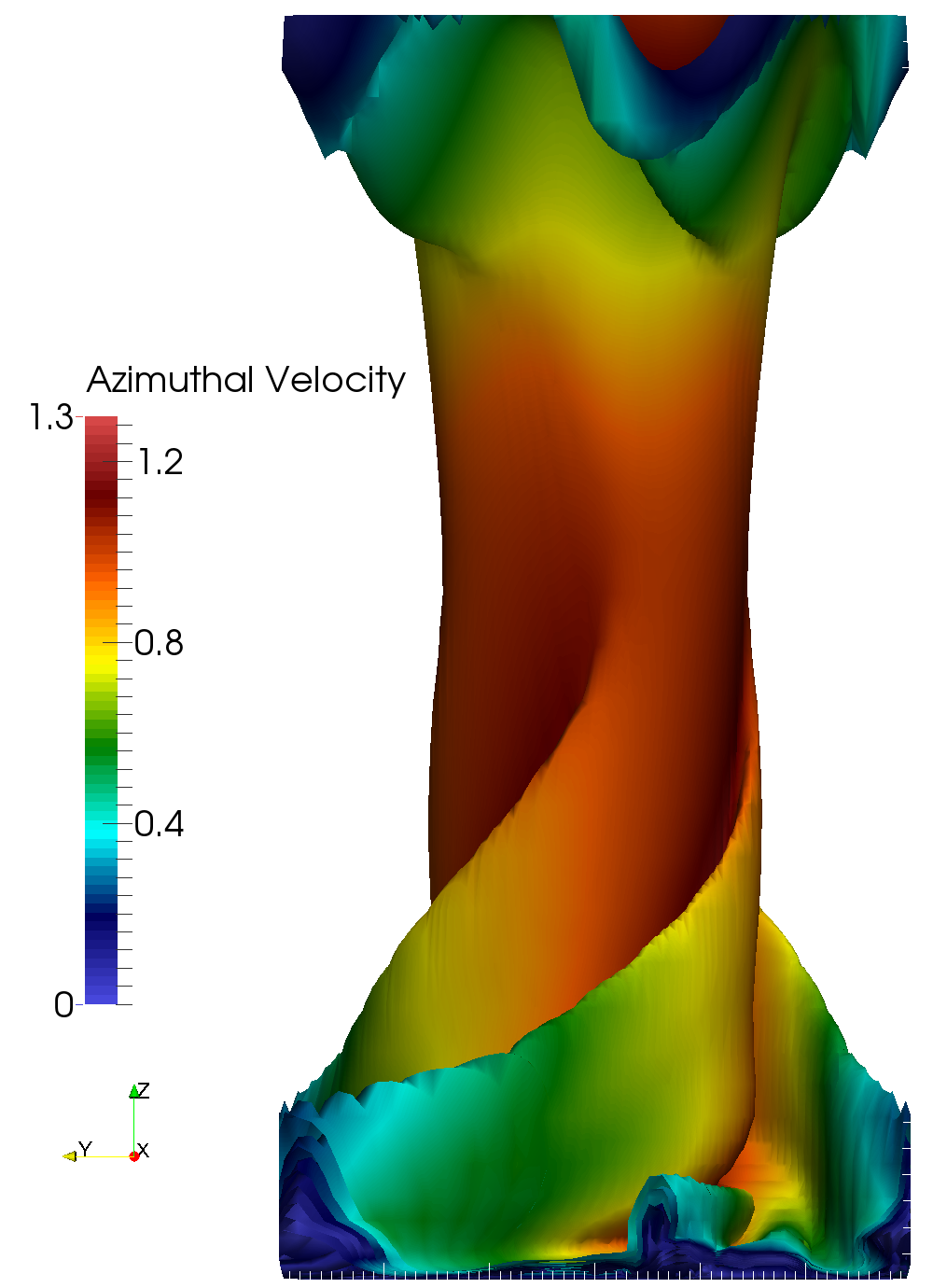
(a) Simulation of thermally induced vortex using incompressible Navier-Stokes, heat transfer, Boussinesq buoyancy, and stabilization Physics operators. Completely specified by user-supplied mesh and input file. Figure provided by Mr. Nicholas Malaya.

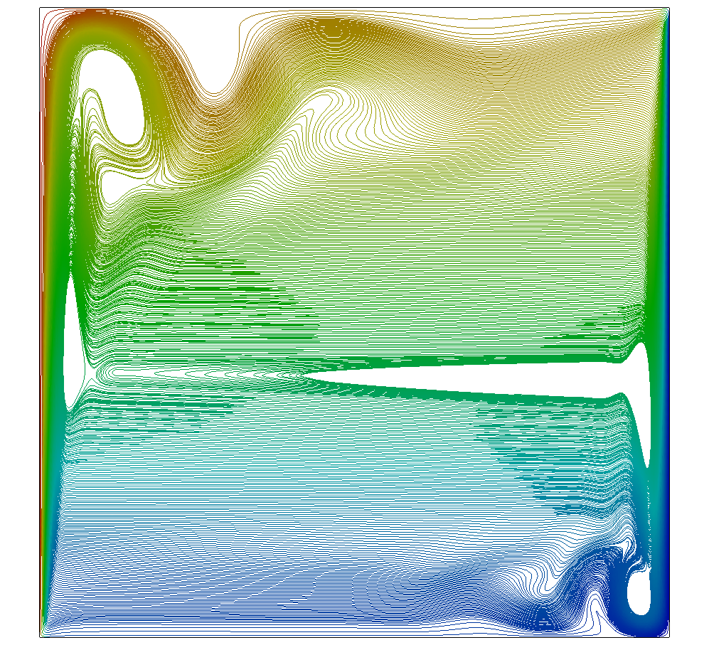
(b) Streamlines, colored by temperature, for cavity benchmark [14] problem. Rayleigh number $Ra=10^{8}$.

Fig. 5: Enabled applications in fluid mechanics.

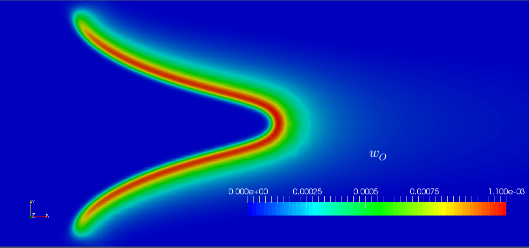
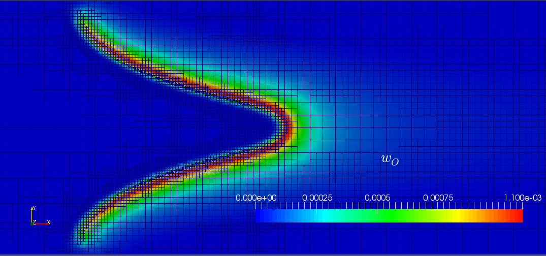
Fig. 6: Example of confined Ozone flame, similar to the example given in Braack et al [15]. Right figure shows mesh adaptation driven by global error indicators.

5.2 Solid Mechanics

Now we describe an application in solid mechanics using this framework. The mathematical models are used to simulate one- and two-dimensional manifolds of elastic materials that undergo large deformation, see e.g. [35]. Although the final application is for modeling of parachutes, we show an example that contains many elements of the desired application whose features illustrate the flexibility of the current work.

The body is a two-dimensional manifold with overlapping one-dimensional “stiffeners” along with the axial directions and pressure distribution acting normal to the surface; the latter induces another geometric nonlinearity in addition to the large deformation. In particular, Figure 7 shows a two-dimensional circular rubber membrane deforming under a uniform pressure loading, acting normal to the surface, with one-dimensional “stiffeners” (cables) along the x- and y-axis. The rubber membrane is modeled as a Mooney-Rivlin material (material nonlinearity) and the cables are modeled as linear elastic materials.

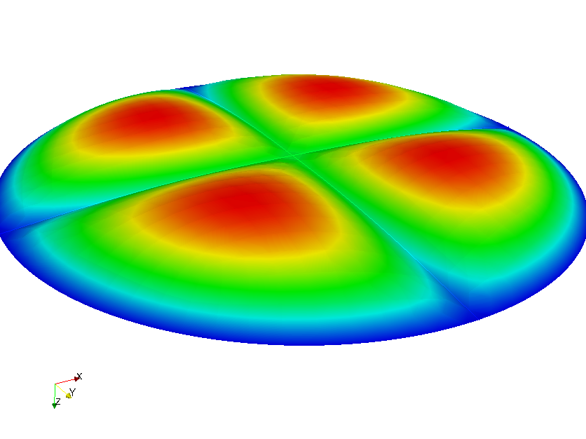
(a) Perspective view of deformed membrane.

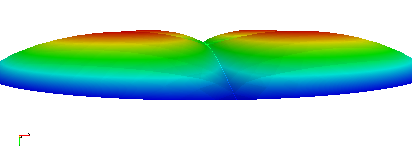
(b) Side view of deformed membrane.

Fig. 7: Deformation of two-dimensional rubber membrane with one-dimensional axial stiffeners. Rubber material is modeled as a Mooney-Rivlin material while the cables are linearly elastic (Hookean).

This application exhibits multiple materials, multiple dimensional mesh elements directly coupled, and the underlying nonlinear plane stress elasticity equations are posed on the manifolds. The latter two elements, to best of the authors knowledge, are challenging to deploy within the FEniCS platform.

This example can use both an unsteady solver with heavy damping or simple continuation solver extension where the applied pressure is incrementally increased. The latter is distributed as part of this example in GRINS and required roughly 100 lines of code.

5.3 QoI-Driven Mesh Adaptivivty

This example illustrates using the QoI and Solver infrastructure to enable QoI-based AMR using error estimates based on adjoint solutions. This particular example mimics that of Prudhomme and Oden [45, 46] for point-valued QoIs, namely the Poisson equation with a prescribed loading such that the solution is a given function.

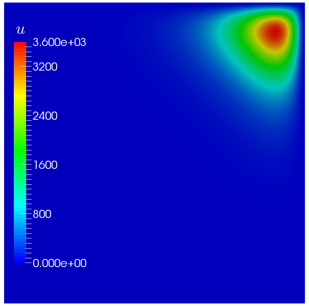
(a) Forward solution.

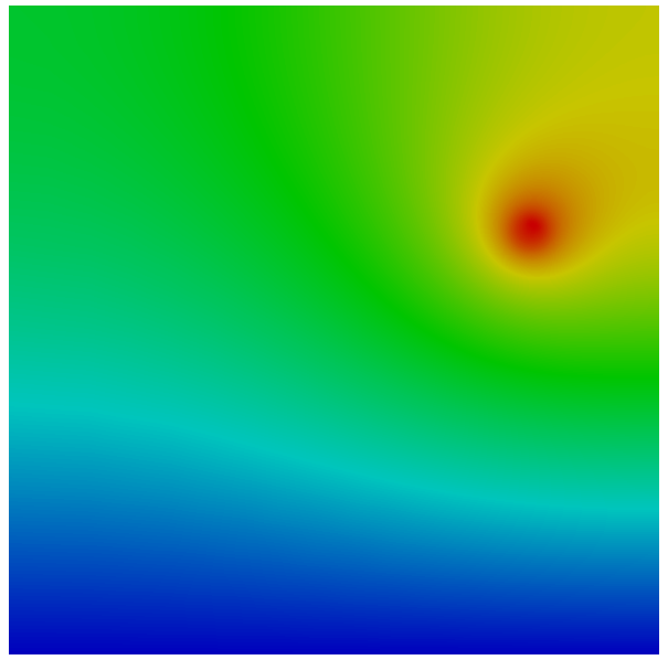
(b) Adjoint solution.

Fig. 8: Forward and adjoint solution for $u(0.8,0.65)$ QoI of Poisson equation.

We note that the infrastructure automatically supports multiple QoIs for both error estimation/adaptive mesh refinement and for parameter sensitivity.

5.4 Data Reduction Modeling

The final set of examples that we cite here are the initial integration with the QUESO statistical library [44] for solving statistical inverse problems. In particular, all of these examples use GRINS as a data reduction model — mathematical models are used to infer desired quantities from experiments given physical measured data and its associated uncertainty.

The first application was using one-dimensional models of thermocouple gages to infer surface heat flux [13]. In this case, the thermal conductivity was unknown and temperature history data was used to infer the conductivity using a Bayesian approach. Several likelihood models were considered, all using the underlying forward model infrastructure. The second application was the real-time inference of a damage field given given strain field measurements [42, 43]. Here, an extended Kalman filter approach was used to update the damage predictions based on measured strain data; the underlying forward model in GRINS supplied to forward model predictions derivatives. The final application is the inference of surface chemistry parameters [12]. This case uses a two-dimensional reacting flow model to study the consumption of carbon by dissociated nitrogen from which surface chemistry between carbon and nitridation can be inferred. Such reactions are important in reentry flows [50].

At this point, all the previous examples are small application codes built using GRINS and QUESO. Current work is providing direct interfaces to QUESO that will facilitate runtime selection of parameters and construction of data reduction models without the need for separate applications. Completion of this work will be the subject of future publications.

6 Concluding Remarks and Future Directions

In this paper, we have described the GRINS multiphysics framework that provides a platform for constructing numerical approximations of complex mathematical models and facilitating the use of modern numerical methods, including adjoint-based error estimation, AMR, and interactions with statistical libraries for performing inference. Users can directly use existing functionality to run calculations only from an input file and supplied mesh and experiment with the solvers and parameters to find the right method for the problem; we were particularly inspired by the PETSc library for this approach. The approach taken here is attempt to balance between infrastructure mandates, e.g. as in FEniCS, and the flexibility afforded by building a stand-alone application.

Ongoing work includes building interfaces between PETSc and libMesh to facilitate the use of adapted grids for geometric multigrid based solvers, building reusable interfaces to QUESO to facilitate rapid deployment of inference applications, more flexibility to interfaces to allow user-specified adjoint operators, infrastructure to support arbitrary Lagrangian-Eulerian (ALE) fluid-structure interaction, as well as many other fine-grained enhancements to lower the barrier for users.

References

- [1] \urlhttps://github.com/gahansen/Albany
- [2] \urlhttp://www.openfoam.org.
- [3] \urlhttp://warp.povusers.org/FunctionParser/.
- [4] \urlhttps://github.com/libantioch/antioch
- [5] \urlhttp://getpot.sourceforge.net/documentation-index.html
- [6] \urlhttp://www.fmrl.gatech.edu/drupal/projects/solarvortex
- [7] Martin S. Alnæs, Anders Logg, Kristian B. Ølgaard, Marie E. Rognes, and Garth N. Wells, Unified form language: A domain-specific language for weak formulations of partial differential equations, ACM Trans. Math. Softw., 40 (2014), pp. 9:1–9:37.
- [8] Satish Balay, Mark F. Adams, Jed Brown, Peter Brune, Kris Buschelman, Victor Eijkhout, William D. Gropp, Dinesh Kaushik, Matthew G. Knepley, Lois Curfman McInnes, Karl Rupp, Barry F. Smith, and Hong Zhang, PETSc users manual, Tech. Report ANL-95/11 - Revision 3.4, Argonne National Laboratory, 2013.
- [9] , PETSc Web page. \urlhttp://www.mcs.anl.gov/petsc, 2014.
- [10] Satish Balay, William D. Gropp, Lois Curfman McInnes, and Barry F. Smith, Efficient management of parallelism in object oriented numerical software libraries, in Modern Software Tools in Scientific Computing, E. Arge, A. M. Bruaset, and H. P. Langtangen, eds., Birkhäuser Press, 1997, pp. 163–202.
- [11] W. Bangerth, R. Hartmann, and G. Kanschat, deal.II – a general purpose object oriented finite element library, ACM Trans. Math. Softw., 33 (2007), pp. 24/1–24/27.
- [12] Paul T. Bauman, Enabling the statistical calibration of active nitridation of graphite by atomic nitrogen, in 45th AIAA Thermophysics Conference, 2015.
- [13] Paul T. Bauman, Jeremy Jagodzinski, and Benjamin S. Kirk, Statistical calibration of thermocouple gauges used for inferring heat flux, in 42nd AIAA Thermophysics Conference, AIAA 2011-3779, 2011.
- [14] R. Becker and M. Braack, Solution of a stationary benchmark problem for natural convection with large temperature difference, International Journal Of Thermal Sciences, 41 (2002), pp. 428–439.
- [15] R. Becker, M. Braack, and R. Rannacher, Numerical simulation of laminar flames at low Mach number by adaptive finite elements, Combustion Theory And Modelling, 3 (1999), pp. 503–534.
- [16] Roland Becker and Rolf Rannacher, An optimal control approach to a posteriori error estimation in finite element methods, Acta Numerica, 10 (2001), pp. 1–102.
- [17] Jed Brown, Matthew G. Knepley, David A. May, Lois Curfman McInnes, and Barry Smith, Composable linear solvers for multiphysics, in Proceedings of the 2012 11th International Symposium on Parallel and Distributed Computing, ISPDC ’12, Washington, DC, USA, 2012, IEEE Computer Society, pp. 55–62.
- [18] J. Brown, M. G. Knepley, D. A. May, Lois Curfman McInnes, and B. F. Smith, Composable linear solvers for multiphysics, in 11th International Symposium on Parallel and Distributed Computing, Munich, Germany, 06/2012 2012.
- [19] P. Brune, M. G. Knepley, B. F. Smith, and X. Tu, Composing scalable nonlinear algebraic solvers, (2013).
- [20] Qiushi Chen, Jakob T. Ostien, and Glen Hansen, Development of a used fuel cladding damage model incorporating circumferential and radial hydride responses, Journal of Nuclear Materials, 447 (2014), pp. 292–303.
- [21] E. Cyr, J. Shadid, and T. Wildey, Approaches for Adjoint-Based A Posteriori Analysis of Stabilized Finite Element Methods, SIAM J. Sci. Comput., 36 (2014), pp. A766–A791.
- [22] A. Dedner, R. Klöfkorn, M. Nolte, and M. Ohlberger, A generic interface for parallel and adaptive scientific computing: Abstraction principles and the dune-fem module, Computing, 90 (2011), pp. 165–196.
- [23] P. E. Farrell, D. A. Ham, S. W. Funke, and M .E. Rognes, Automated derivation of the adjoint of high-level transient finite element programs, SIAM J. on Sci. Comput., 35 (2013), pp. C369––C393.
- [24] Erich Gamma, Richard Helm, Ralph Johnson, and John Vlissides, Design Patterns: Elements of Reusable Object-Oriented Software, Addison-Wesley Professional, 1 ed., 1994.
- [25] Vikram V. Garg, Coupled Flow Systems, Adjoint Techniques and Uncertainty Quantification, PhD thesis, The University of Texas at Austin, 2012.
- [26] D. R. Gaston, C. J. Permann, D. Andrs, and J. W. Peterson, Massive hybrid parallelism for fully implicit multiphysics, in Proceedings of the International Conference on Mathematics and Computational Methods Applied to Nuclear Science & Engineering (M&C 2013), May 5–9, 2013.
- [27] D. R. Gaston, C. J. Permann, J. W. Peterson, A. E. Slaughter, D. Andrš, Y. Wang, M. P. Short, D. M. Perez, M. R. Tonks, J. Ortensi, and R. C. Martineau, Physics-based multiscale coupling for full core nuclear reactor simulation, Annals of Nuclear Energy, Special Issue on Multi-Physics Modelling of LWR Static and Transient Behaviour, 84 (2015), pp. 45–54. \urlhttp://dx.doi.org/10.1016/j.anucene.2014.09.060.
- [28] D. G. Goodwin, An open-source, extensible software suite for cvd process simulation, in CVD XVI and EuroCVD Fourteen, M. Allendorf, F. Maury, and F. Teyssandier, eds., Electrochemical Society, pp. 155–162.
- [29] Max .D. Gunzburger, Finite Element Methods for Viscous Incompressible Flows, Academic Press, 1989.
- [30] C. H. Hamilton and A. Rau-Chaplin, Compact hilbert indices: Space-filling curves for domains with unequal side lengths, Information Processing Letters, 105 (2008), pp. 155–163.
- [31] Michael A. Heroux, Roscoe A. Bartlett, Vicki E. Howle, Robert J. Hoekstra, Jonathan J. Hu, Tamara G. Kolda, Richard B. Lehoucq, Kevin R. Long, Roger P. Pawlowski, Eric T. Phipps, Andrew G. Salinger, Heidi K. Thornquist, Ray S. Tuminaro, James M. Willenbring, Alan Williams, and Kendall S. Stanley, An overview of the trilinos project, ACM Trans. Math. Softw., 31 (2005), pp. 397–423.
- [32] George Karypis and Vipin Kumar, A fast and highly quality multilevel scheme for partitioning irregular graphs, SIAM Journal on Scientific Computing, 20 (1999), pp. 359–392.
- [33] Benjamin S. Kirk, Adaptive Finite Element Simulation of Flow and Transport Applications on Parallel Computers, PhD thesis, The University of Texas at Austin, 2007.
- [34] B. S. Kirk, J. W. Peterson, R. H. Stogner, and G. F. Carey, libMesh: A C++ library for parallel adaptive mesh refinement/coarsening simulations, Engineering with Computers, 22 (2006), pp. 237–254.
- [35] Alain Lo, Nonlinear Dynamic Analysis of Cable and Membrane Structures, PhD thesis, Oregon State University, 1982.
- [36] Anders Logg, Kent-Andre Mardal, and Garth Wells, eds., Automated Solution of Differential Equations by the Finite Element Method, vol. 84 of Lecture Notes in Computational Science and Engineering, Springer, 2012.
- [37] J. Nocedal and S. J. Wright, Numerical Optimization, Springer, New York, 1999.
- [38] J. T. Oden and S. Prudhomme, Estimation of modeling error in computational mechanics, Journal Of Computational Physics, 182 (2002), pp. 496–515.
- [39] J. T. Oden, S. Prudhomme, A. Romkes, and P. T. Bauman, Multiscale modeling of physical phenomena: Adaptive control of models, SIAM Journal on Scientific Computing, 28 (2006), pp. 2359–2389.
- [40] John W. Peterson, Parallel Adaptive Finite Element Methods for Problems in Natural Convection, PhD dissertation, The University of Texas at Austin, 2008.
- [41] J. Principe and R. Codina, Mathematical models for thermally coupled low speed flows, Advances in Theoretical and Applied Mechanics, 2 (2009), pp. 93–112.
- [42] E. E. Prudencio, P. T. Bauman, D. Faghihi, K. Ravi-Chandar, and J. T. Oden, A computational framework for dynamic data-driven material damage control, based on bayesian inference and model selection, Int. J. Numer. Meth. Engng, 102 (2015), pp. 379–403.
- [43] E. E. Prudencio, P. T. Bauman, S. V. Williams, D. Faghihi, K. Ravi-Chandar, and J. T. Oden, Real-time inference of stochastic damage in composite materials, Composites Part B: Engineering, 67 (2014), pp. 209–219.
- [44] Ernesto E. Prudencio and Karl W. Schulz, The parallel C++ statistical library QUESO: Quantification of uncertainty for estimation, simulation and optimization, in Euro-Par 2011 Workshops, Part I, M. Alexander et al., ed., vol. 7155 of Lecture Notes in Computer Science, Springer-Verlag, Berlin Heidelberg, 2012, pp. 398–407.
- [45] S. Prudhomme and J. T. Oden, On goal-oriented error estimation for elliptic problems: application to the control of pointwise errors, Computer Methods in Applied Mechanics and Engineering, 176 (1999), pp. 313–331.
- [46] Serge Michael Prudhomme, Adaptive Control of Error and Stability of h-p Approximations of the Transient Navier-Stokes Equations, PhD thesis, University of Texas at Austin, 1999.
- [47] James Reinders, Intel Threading Building Blocks: Outfitting C++ for Multi-core Processor Parallelism, O’Reilly Media, 2007.
- [48] Alan Shalloway and James R. Trott, Design Patterns Explained, Addison-Wesley, 2 ed., 2005.
- [49] JR Stewart and HC Edwards, A framework approach for developing parallel adaptive multiphysics applications, Finite Elements In Analysis And Design, 40 (2004), pp. 1599–1617.
- [50] R. Stogner, Paul T. Bauman, K. W. Schulz, and R. Upadhyay, Uncertainty and parameter sensitivity in multiphysics reentry flows, in 49th AIAA Aerospace Sciences Meeting, AIAA 2011-764, 2011.
- [51] Roy H Stogner, Parallel Adaptive C1 Macro-Elements for Nonlinear Thin Film and Non-Newtonian Flow Problems, PhD thesis, The University of Texas at Austin, 2008.
- [52] Roy H Stogner and Graham F Carey, C-1 macroelements in adaptive finite element methods, International Journal for Numerical Methods in Engineering, 70 (2007), pp. 1076–1095.
- [53] Roy H Stogner, Graham F Carey, and Bruce T Murray, Approximation of Cahn-Hilliard diffuse interface models using parallel adaptive mesh refinement and coarsening with C-1 elements, International Journal for Numerical Methods in Engineering, 76 (2008), pp. 636–661.
- [54] I. Tezaur, A. Salinger, M. Perego, and R. Tuminaro, On the development & performance of a first order stokes finite element ice sheet dycore built using trilinos software components, in SIAM Conference on Computational Science and Engineering, Salt Lake City, UT, 2015.
- [55] T. M. van Opstal, Paul T. Bauman, Serge Prudhomme, and E. H. van Brummelen, Goal-oriented adaptive modeling for viscous incompressible flows, (2013). ICES Report 13-07.
- [56] Min Zhou, Onkar Sahni, Ting Xie, Mark S. Shephard, and Kenneth E. Jansen, Unstructured mesh partition improvement for implicit finite element at extreme scale, The Journal of Supercomputing, 59 (2012), pp. 1218–1228.